Louisiana State UniversityLSU Digital Commons

LSU Historical Dissertations and Theses Graduate School

1967

A Theoretical Study of the Force Exerted by aViscous Fluid on an Oscillating Cylinder.John Stephen BosnakLouisiana State University and Agricultural & Mechanical College

Follow this and additional works at: https://digitalcommons.lsu.edu/gradschool_disstheses

This Dissertation is brought to you for free and open access by the Graduate School at LSU Digital Commons. It has been accepted for inclusion inLSU Historical Dissertations and Theses by an authorized administrator of LSU Digital Commons. For more information, please contactgradetd@lsu.edu.

Recommended CitationBosnak, John Stephen, "A Theoretical Study of the Force Exerted by a Viscous Fluid on an Oscillating Cylinder." (1967). LSUHistorical Dissertations and Theses. 1322.https://digitalcommons.lsu.edu/gradschool_disstheses/1322

This dissertation has been microfilmed exactly as received 67—17,305

BOSNAK, John Stephen, 1941- A THEORETICAL STUDY OF THE FORCE EXERTED BY A VISCOUS FLUID ON AN OSCILLATING CYLINDER.

Louisiana State University and Agricultural and Mechanical College, Ph.D., 1967 P hysics, general

University Microfilms, Inc., Ann Arbor, Michigan

A THEORETICAL STUDY OF THE FORCE EXERTED BY A VISCOUS FLUID ON AN OSCILLATING CYLINDER

A Dissertation

Submitted to the Graduate Faculty of the Louisiana State University and

Agricultural and Mechanical College in partial fulfillment of the requirements for the degree of

Doctor of Philosophy

in

The Department of Physics and Astronomy

byJohn Stephen Bosnak

B.S.,Missouri School of Mines and*Metallurgy, 1963August, 1967

ACKNOWLEDGEMENT

The author wishes to express his gratitude to Dr. Robert G. Hussey for his assistance and guidance in this project. He thanks his wife and children for their encouragement and patience during the period of his grad­uate study. The author is indebted to his parents for their moral and financial support in the furthering of his education. He wishes "to acknowledge the financial aid received from the Dr. Charles E. Coates Memorial Fund of the L. S. U. Foundation donated by George H. Coates for the expenses of preparation of this dissertation.

TABLE OF CONTENTS

PageI. INTRODUCTION ..................................... 1

II. PERTURBATION SOLUTION FOR A CYLINDER PERFORMING ANGULAR OSCILLATIONS INAN INFINITE FLUID .............................. ~21

III. SEPARATION MODELS .............................. 67IV. RESULTS AND CONCLUSIONS ....................... 98

REFERENCES ............................................ 103APPENDIX

Calculation of Ak and Akf from the Force Exerted on the Cylinder by the Fluid During S e p a r a t i o n ....................................... A-l

VITA .................................... 107

iii

LIST OF FIGURES

Figure Page1. Kimball's Torsion Pendulum Apparatus . . . . 72. Kimball’s A k 1 Results for Several Fluids . . 93. Kimball's Ak Results for Several Fluids . . 104. Boundary Effect for Carbon Tetrachloride . . 125. Schlichting's Theoretical Steady

Streaming Flow Pattern .................156 . The Universal Curve Expressing as a

Function of a/SAC ................ . . . . . 187. Flow about a Circular Cylinder as

Viewed in the Rest Frame of the Cylinder . . 208 . Flow, with Separation, about a

Circular Cylinder .......................... 2 29. Notation for the Angular Oscillating

Cylinder .......................................... 2810. Notation for Cylinder Performing

Linear Translational Oscillations ......... 6911. Assumed Time Dependence of the

Separation Angle ............................. 7 712. Experimental Values of Ak' vs. Potential

Flow Model Values of Ak'/K......................... 8013. Comparison of Experimental and Potential

Flow Model Values of Ak . 8 214. Experimental Values of Ak’ vs. Viscous

Flow Model Values of Ak’/K . ...................9515. Comparison of Experimental and Viscous

Flow Model Values of -7 — Ak ................... 9 6

iv

ABSTRACT

When a circular cylinder performs free translational sinusoidal oscillations in a viscous fluid, the force exerted on the cylinder by the fluid causes damping and a change in the period of oscillation. The damping and change in period can be expressed in terms of a damping parameter, k* , proportional to the logarithmic decrement, and a period parameter, k, proportional to the change of the period.These parameters were first introduced by Stokes in his study of the low amplitude oscillations of a cylinder in a viscous fluid.

If the amplitude of oscillation is much smaller than the cylinder radius, k' and k are independent of amplitude; but experiments indicate that for high amplitudes k' and k are amplitude dependent.. In this study it is shown that the change, Akr, in the damping parameter with amplitude of oscillation can be explained by a simple flow model based on the assumed occurrence of separation when the amplitude ex-

I.ceeds t'Ji, where A is the viscous penetration depth and a is the cylinder radius. Two separation models are presented: a potential flow model and a viscous flow model. The ex­pression obtained for Ak1 from the potential flow model is

Ms 1 “ l “s (cont’d)a)

aki = M-C0.16) -4-- sinwt {-0 2 a/Aa s3 IT

V

/Tawhere A is the amplitude of oscillation, cosut = 1 - — *2 ojt s A

and a) /u = 1 - ---- . The viscous flow model gives abouts IIthe same results for Ak'. The separation models predict a decrease in the period parameter with increasing amplitude, but the predicted decrease is much smaller than that ob­served experimentally.

A low amplitude perturbation solution of the Navier- Stokes equations is obtained for a cylinder oscillating sinusoidally along the arc of a circle in a viscous fluid. Expressions for k and k 1 for this type of motion are foundto be (for x<<a)

i ,3 2 , 3k * 1 + 2 r + 7T + rr<s - i f V8 a b a

. .2 . 3 2 . Q .22 I + V A + 77 <1+ rr+ w Va 8a b 2a a

where b is the radius of the circular arc along which the2 2motion takes place, the terms having a /b as coefficient

are the contributions of the rotational part of the motion, and the other terms are the contributions, found by Stokes, of the translational part of the motion. The stream

vii

function is obtained to second order in amplitude, and particular attention is given the time independent part (steady streaming) of the second order terms. It is found that the steady streaming velocity components caused by the interaction of the translational and rotational motions do not vanish at large distances from the cylinder. Moreover, it is shown that all second order terms have no effect on k and k 1.

CHAPTER I

INTRODUCTION

The primary subject of this study is the force exerted by a viscous fluid upon a circular cylinder performing trans­lational sinusoidal oscillations in the fluid. The first detailed theoretical study of this problem was made by Stokes,'1' whose interest lay in the force on the supporting wires of pen-dula moving in air. In recent years renewed interest has been

2 3generated in this problem * because of the presence of several nonlinear effects, one of which is the phenomenon of steady streaming. Steady streaming is a type of steady, or time in­dependent , fluid flow induced in a fluid by an unsteady oscillatory flow in the presence of a bounding surface.

14For low amplitude oscillations Stokes showed that the force on an oscillating cylinder could be written in the form

(1-1 ) F = - M 1ky - w M 1k 1y

where M ’ is the mass of fluid displaced by the cylinder, <u is the angular frequency of oscillation, y is the cylinder accel­eration, y is the cylinder velocity, and k and k ’ are dimen- sionless parameters depending on fluid properties, cylinder radius, and period of oscillation. For free oscillations the part of the force proportional to the cylinder acceleration affects the period of oscillation and the part proportional to the velocity causes damping. Hence the parameters k and k 1

2

may be referred to as the period parameter and damping parameter, respectively.

The effects of the fluid upon the period and damping have previously been studied both experimentally and theo­retically for the case of small amplitude of oscillation. Although experimental results for high amplitudes have been obtained, no quantitative explanation for those results hasbeen offered. The phenomenon of separation has been sus-

5 6pected to be associated with the high amplitude results. ’It is the purpose of this study to attempt to take intoaccount the effects of separation in as simple a manner as.possible and to see if these effects satisfactorily accountfor experimental observations. .In addition, it is desiredto find the effects of steady streaming on the force exertedon the cylinder by the fluid.

The following topics will be discussed in this chapter:(A) the theoretical low amplitude results of Stokes;(B) a summary, of previous experimental results for k and k r

at low and high amplitudes of oscillation;(C) a summary of previous theoretical and experimental re­

sults for steady streaming;(D) the manner in which separation comes about and examples

of separation in fluid flow about cylinders;(E) the reasons for suspecting connections between high

amplitude results for k and k f and the phenomena of separation and steady streaming.

7 8(A) The Theoretical Low Amplitude Results of Stokes *

Stokes studied the problem of a circular cylinderperforming sinusoidal oscillations along a diameter in aninfinite, viscous, incompressible fluid. His theory is

grestricted by two conditions:1. The amplitude of oscillation, A, must be much

smaller than the cylinder radius, a;2. The viscous, penetration depth, A , must be much

1/2smaller than the cylinder radius. (X = (2v/iu) , where vis the kinematic viscosity of the fluid and u is the angular frequency of oscillation.)

The equations governing the motion'of a viscous, incompressible fluid are

(l-2a) + (v-V)v = - — Vp + vV^v3t P

(l-2b) V-v = 0

where v is the fluid velocity, p is the fluid density, and p is the pressure. Equations (1-2) are called the Navier- Stokes equations. Under the restrictions stated above, the nonlinear term (v*V)v may be neglected in Eq. (l-2a). The boundary conditions are that the fluid must adhere to the cylinder surface, i.e. at the cylinder surface v = velocity of the cylinder, and the fluid velocity must vanish at infinite distances from the cylinder. Stokes applied the boundary condition at the cylinder surface at the mean position of the cylinder. This approximation is valid

1+

under the restriction A << a as will be seen from the results of Chapter II.

After solving Eqs. (1-2) for the fluid velocity and pressure, Stokes calculated the force exerted on the cylinder by the fluid and found that it could be expressed in the form given by Eq. (1-1). When this force is placed in the equation of motion of the cylinder it is found that for free oscilla­tions the parameters k and k 1 can be related to the period and damping in the following manner (for small damping):

r 2 2»Ot(T “ T 0 )(l-3a) k = jp---

(l-3b) k ' =

where t is the period of oscillation,tq is that value the2period would have if the motion took place in vacuum, 4tt a

is the force constant associated with the linear restoring force, and D is the logarithmic decrement.

The period and damping parameters can be expressed interms of the penetration depth and cylinder radius in the following manner:^

i + H ^ U m a )(l-4a) k = 1 - RE [— ± ^ — ■— ]

ima H0 (ima)

(ima)(l-4b) k' = IM [----- pr-r--- ]

ima Hq (ima)

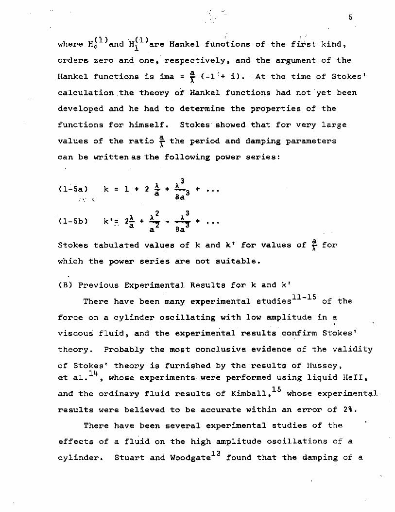
where H o ^ a n d H ^ ^ a r e Hankel functions of the first kind, orders zero and one, respectively, and the argument of the Hankel functions is ima = ^ (-1 + i). ''At the time of Stokes1 calculation the theory of Hankel functions had not yet been developed and he had to determine the properties of the functions for himself. Stokes showed that for very large values of the ratio ^ the period and damping parameters can be written as the following power series:

X X3(l-5a) k = 1 + 2 4- + — - + ... v c a 8a

2 3(1-Sb) k 1 = 2*- + K + ...

a a 8aStokes tabulated values of k and k f for values of ^ for which the power series are not suitable.

(B) Previous Experimental Results for k and k 111-15There have been many experimental studies of the

force on a cylinder oscillating with low amplitude in at ’

viscous fluid, and the experimental results confirm Stokes1 theory. Probably the most conclusive evidence of the validity of Stokes1 theory is furnished by the.results of Hussey,Hiet al, , whose experiments were performed using liquid Hell,and the ordinary fluid results of Kimball,15 whose experimentalresults were believed to be accurate within an error of 2%.

There have been several experimental studies of theeffects of a fluid on the high amplitude oscillations of a

13cylinder. Stuart and Woodgate found that the damping of a

6

cylinder oscillating in air increased approximately linearly with increasing amplitude at amplitudes above about 1/10 the

Ccylinder diameter. Keulegan and Carpenter measured the dragcoefficient, CD (proportional to drag force/diameter x vel-ocity ), and inertia coefficient, Cm = k + 1 , of a cylinderheld fixed and immersed in an oscillating water-filled basin.Their results are presented as plots of C., and C vs. a

U T D . “"period parameter", — (not to be confused with k ) , where Umis the amplitude of the oscillatory fluid velocity, x theperiod, and d the diameter of the cylinder. They find thatthe inertia coefficient has a value of about 2 for very smallvalues of their period parameter, falls to a minimum value of

U T1 at — r— = 15, and then increases to a value of about 2.5 atii dU x—-t— = 120. The drag coefficient has a low amplitude value of

U xabout 0.9. and increases to a maximum at the value of =15.dIt then gradually decreases to a value slightly greater than

Um T1 for — =120. The critical value of 15 corresponds to arelative amplitude (amplitude/radius)of about 4.8.

A fairly detailed account of the experimenta± results of 15Kimball will be given here. Kimball measured the changes

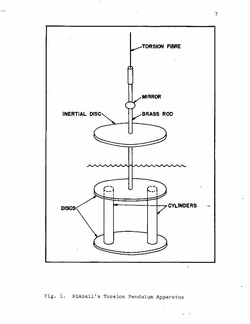
in k and k' with amplitude for cylinders oscillating in several different fluids. His torsion pendulum apparatus is shown in Fig. 1.

Kimball mounted two cylinders made of alloy tubing between two aluminum discs and connected the upper disc to a torsion fibre via a brass.rod. On the rod were fastened an inertial disc (to ensure' small damping) and a small mirror. The disc- cylinder combination was immersed in a fluid and a "twist"

7

TORSION FIBRE

MIRROR

INERTIAL DISC BRASS ROD

CYLINDERSDISCS

Fig. 1. Kimball's Torsion Pendulum Apparatus

8

given the fibre. The resulting amplitude of the free oscillations was measured by reflecting a light beam off the mirror and measuring the deflections of the light beam on a circular scale. Period measurements were made using a photocell connected to an electronic timing device.

Kimball presented his results as plots of the changes, Ak and A k 1, of the period and damping parameters with ampli­tude of oscillation. The kinematic viscosities of thefluids used in his experiments varied from a value of

-2 cm20.2 04 x 10 for liquid nitrogen to a value ofS 6 C- 2 23.625 x 10 cm /sec for aniline. He accounted for the

(small) effects of the discs by measuring the change in theperiod and damping with amplitude for the discs alone andthen subtracting the disc effects from the total.

Kimball's results for Ak' for several fluids (andcylinder radius = 0.64 cm.) are shown in Fig. 2, along with

2a plot of the function 0.4A . The curves show that A k f iszero up to a "critical amplitude" of the order of 1/2 thecylinder radius. Kimball found an empirical relationshipA .. = /\a for the Ak' results. The Ak' results showc n tlittle dependence on kinematic viscosity over the rangeused, and as can be seen from Fig. 2 the curves can be well

2approximated by the function 0.4A .Kimball's results for the changes in k with amplitude

are shown in Fig. 3. The curves show that Ak is zero up to amplitudes slightly higher than the critical amplitudes

1.0 a = o.64gm t = 4.409EC

0.8 -A - CCI4+ - h2o

O - ISOPROPYL ALCOHOL0.6 -

0.4 -Ak'

0.2 -

A tCM.

1.40.6 0.8 1.00.2 0.4

Fig. 2. Kimball's Ak' Results for Several Fluids

- 0.2 - Ak-0.4- IS0PR0PYL ALCOHOL

- 0 .6-CCI

0.8-

A ,CM .

1.2 1.60.80.4

Fig. 3. Kimball's Ak Results for Several Fluids

O

11

for the Ak’ curves. The Ak curves are typified at first by a decrease in Ak with increasing amplitude, the existence of a minimum value of the order of -0.7 at a relative amplitude of about 2.5, and then a gradual increase with continually increasing amplitude.

Kimball experimentally tested the effects of the size of the boundary containing his oscillators on Ak' and Ak and found that Ak' is relatively insensitive to changes in the size of the boundary, while the ak curves are greatly affected by the boundary size, the important dimension being the distance of the boundary from the cylinders.The magnitude of the minima and amplitude at the minimum values in the ak curves were both decreased by moving the boundary closer to the cylinders. The boundary effectupon ak for carbon tetrachloride is shown in Fig. 4.

1. 6Thibodeaux used an apparatus similar to Kimball's to measure the changes in k and k' with amplitude in liquid Hell. He found that at 2.15 K his ak' curves could be fitted by the relationship ak' « 0.17(A/a)^.His critical amplitude relationship is the same as Kimball's but is complicated by the introduction of an "effective" .kinematic viscosity brought about by the interaction of superfluid and normal fluid components of liquid Hell.

CCI4

CL= 0.64GM t = 7.40CM

0.2-

0.4-Ak

0.6 - A= DISTANCE OF BOUNDARY FROM CYLINDERS

0.8-

1.0 -A.CM.

1.2 1.60.4 0.8

Fig. 4. Boundary Effect for Carbon Tetrachloride

13

(C) Previous Theoretical and Experimental Results for Steady Streaming.

As stated previously, steady streaming is a type of steady flow induced in a fluid by an unsteady oscillatory flow in the presence of a bounding surface. The oscilla­tory flow might be caused by a small amplitude sound wave,in which case the steady streaming is referred to as

17 18acoustic streaming, * or by the oscillatory motion of a boundary, the latter case being of particular interest here. The manner in which the steady streaming comes about can be seen by considering an oscillatory flow of small amplitude having as first approximation a fluid velocity of the form v = u(r) cos wt, where r is a general position vector. From Eq. (l-2a) it can be seen that thenonlinear term, (v*V)v, will then be of the form

2 -*■* 1 1 . (u*7)u cos ut' = (u*V)u(-j + cos2wt). The second approxi­mation to the fluid velocity will then contain terms which are independent of time (the steady streaming) and terms having an oscillatory behavior with twice the frequency of the oscillatory first approximation. A physical interpre­tation of the nonlinear terms as virtual stresses, known

19as Reynolds stresses, has been given by Stuart.The first theoretical treatment of the steady streaming

produced by oscillatory flow about a circular cylinder was20made by Schlichting. Schlichting studied the problem

of an infinite circular cylinder oscillating with small

14

amplitude along a diameter in an infinite, viscous,incompressible fluid. By solving the boundary layer

21equations for planar flow he showed that the steady streaming velocity does not vanish at large distances from the cylinder surface (as it should, from the boundary con­ditions). Schlichting found that at large distances fromthe cylinder surface the streaming velocity component

3 duoparallel to the surface has the value - ^ Uog^-— , where x is the coordinate measured parallel to the cylinder surface, and the external potential flow velocity component parallel to the surface is U0 (x) cos a>t. In the streaming flow pattern found by Schlichting, the fluid flows away

Urnfrom the cylinder in both directions parallel to the cylinder motion, and toward the cylinder in both directions perpendicular to the cylinder motion (see Fig. 5).

The experimental streaming directions observed by2 2 23Andrade and Schlichting were in agreement with

24Schlichting1s theory, but others (Carriere, Andres and 18Ingard ) observed streaming in the opposite direction.

The controversy was apparently resolved by the work ofn c o e

Holtsmark, et al., and that of Raney, et al. The Holtsmark group presented a perturbation solution of the Navier-Stokes equations for a fixed cylinder in an oscil­lating stream. Their streaming solutions exhibit the samequalitative features as Schlichting's except their streaming

27velocities vanish at large distances from the cylinder.

15

Fig. 5. Schlichting's Theoretical Steady Streaming Flow Pattern ( Symmetric in All Quadrants )

16

They introduced the concept of a steady streaming boundary»layer thickness, defined as that distance from the

cylinder at which the radial component of the streaming velocity first vanishes, and measured 6D(_, for air oscil­lating about a fixed cylinder. They observed that outside the steady streaming boundary layer the streaming is directed away from the cylinder in both directions parallel to the cylinder motion and toward the cylinder in both directions perpendicular to the cylinder motion; inside the streaming boundary layer the streaming has the opposite sense. Their experimental values of 6^^ were smaller than the values predicted by their theory but larger than those predicted by Schlichting's theory.

The agreement between experimental and theoretical2 6 *values of 6^ was improved by Raney, et al., who modified

the Holtsmark calculation by expressing the steady streaming velocities in Lagrangian coordinates. The need to use

2 8Lagrangian coordinates had been pointed out by Westervelt, who observed that experimental observations of steadystreaming were made by measuring the time average velocitiesof fluid particles (hence, Lagrangian velocities), whiletheoretical calculations were made in Eulerian coordinates.Raney, et a l ., measured streaming boundary layer thicknessesover a wide range of kinematic viscosity by using mixturesof glycerin and water, and they found that their theoreticalvalues of 6^^ agreed much better with the experimentalvalues than did the theoretical values of the Holtsmark group.

17

Raney, et a l ., also presented an empirical universal curveexpressing 5 q as a function of the cylinder radius, a, and

1/2the "AC" boundary layer thickness 6^ = (v/w) (see Fig. 6). The universal curve shows that fij)Q/a is a function only of a/6ac* For smaii values of a/ ^ c ‘t ie curve shows thatSD£,/a is large. The Raney group pointed out that the ex-

24 18periments of Carriere and Andres and Ingard had beenperformed at small values, = 8 , of a /5^Q* The direction of streaming (toward the cylinder along both directions parallel to the cylinder motion) observed by Carriere and Andres and Ingard was probably that of the streaming inside the streaming boundary layer (see Fig. 5). The Raney group also presented experimental plots of 6^ vs. A/6^ (amp­litude/5^) which show that for A/6^^>lthe streaming boundary layer thickness is amplitude dependent. Their universal curve (Fig. 6) is then valid only for A/^<1.Their curves showing the amplitude dependence of 6DC arestrongly dependent on cylinder radius.

2 9Skavlem and Tjotta calculated the streaming velocities for one cylinder oscillating inside another. Their calcu­lation is valid only for A/5^^.<1, and they find that 6^c (for the inner cylinder)is unaffected if the radius of the outer cylinder is much larger than that of the inner.

18

1 0 0 0 -

500-

2.00-

i.oo-

0.20-

0 .10-

0.05-

0.0210 4020 30 50

Fig. 6. The Universal Curve Expressing asa Function of a/6^

19

3 0Westervelt has found an equation expressing as a function of a/6^c :

13(2)^^ ^AC 13(2)^^ ^AC■ W a = [ a - ^ t 2- -- 12 ' -i>C2-lM|i— ] -AS.His equation fits the universal curve (Fig. 6) very welldown to a/<5^£= 13 ( 2 3 .

oStuart has made a boundary layer theory investigation of steady streaming about a circular cylinder. He noted that from Schlichting1s theory a characteristic streaming velocity is V = t W w d (from a dimensional analysis con-

Q JTIsideration of Schlichting's - ^ UQ flx,g ), where is theamplitude of the oscillatory velocity, u> is the angularfrequency, and d is the diameter of the cylinder. Then aReynolds number for the steady streaming is

2R = Vd/v = U /uv. The velocity amplitude and amplitude s ®of oscillation are related by the expression = w A, so

2 2 that Rg= A /(v/w) = (A/6a c > , the square of the parameterused by Raney, et al. For large values of R Stuartshowed that outside the oscillatory (inner) boundary layer,6a c , there is an outer layer within which the streamingvelocity component parallel to the cylinder surface decaysto zero. The thickness of this outer layer is approximately

1/2d(ujv) /U^ and is large compared with 6^c but small compared with d. Stuart's theory is.valid only for A<<d, S^£<<d, and large values of R g . The connection

20

(if one exists) between Stuart’s outer layer and the steady streaming boundary layer is not clear.

It should be remarked here also that the forces exerted on the cylinder calculated using boundary layertheory do not agree with Stokes' force. The discrepancy

31 3 2has been studied by Segel and by Stuart.

(D) S e p a ration^^^

The phenomenon of separation may be described by con­sidering fluid flow about a circular cylinder as viewed inthe rest frame of the cylinder. The flow pattern may be

3 5described by considering two distinct regions:1 . A thin boundary layer next to the cylinder surface in which the fluid encounters large viscous forces;2. The region outside the boundary layer, where viscous forces are not important and the fluid flow is frictionless potential flow.

Fig. 7. Flow about a Circular Cylinder as Viewed in the Rest Frame of the Cylinder., (No Separation)

21

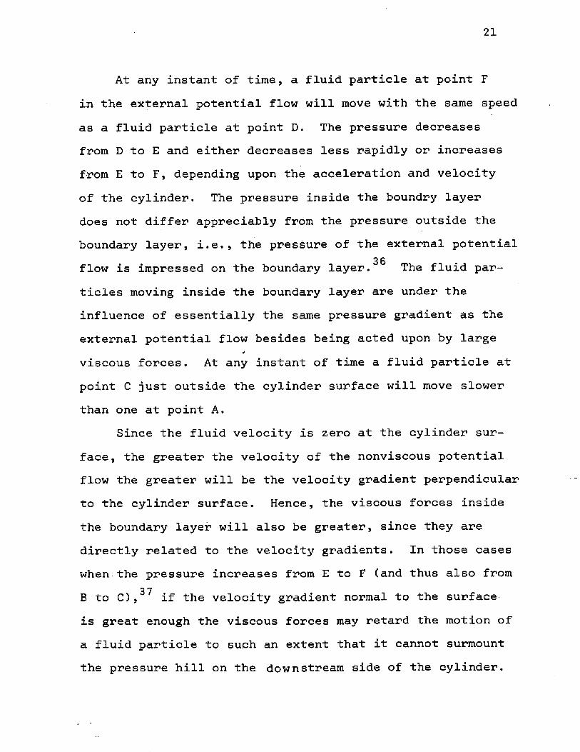
At any instant of time, a fluid particle at point Fin the external potential flow will move with the same speedas a fluid particle at point D. The pressure decreasesfrom D to E and either decreases less rapidly or increasesfrom E to F, depending upon the acceleration and velocityof the cylinder. The pressure inside the boundry layerdoes not differ appreciably from the pressure outside theboundary layer, i.e., the pressure of the external potential

3 6flow is impressed on the boundary layer. The fluid par­ticles moving inside the boundary layer are under the influence of essentially the same pressure gradient as theexternal potential flow besides being acted upon by large

*viscous forces. At any instant of time a fluid particle at point C just outside the cylinder surface will move slower than one at point A.

Since the fluid velocity is zero at the cylinder sur­face, the greater the velocity of the nonviscous potential flow the greater will be the velocity gradient perpendicular to the cylinder surface. Hence, the viscous forces inside the boundary layer will also be greater, since they are directly related to the velocity gradients. In those caseswhen the pressure increases from E to F (and thus also from

3 7B to C), if the velocity gradient normal to the surface is great enough the viscous forces may retard the motion of a fluid particle to such an extent that it cannot surmount the pressure hill on the downstream side of the cylinder.

22

The particle's component of velocity parallel to the cylinder surface is arrested. The external pressure then forces the particle to move in the opposite direction. The boundary layer thickens on the downstream side of the cylinder and boundary layer material flows into the outside region. This loss of boundary layer material into the external region of flow is called separation.

Fig. 8 . Flow, with separation, about a circularcylinder. Points labelled S represent points of separation, and 6 is the separation angle.

As the fluid velocity component parallel to the cylinder surface is arrested and the velocity at the cylinder surface is zero, there will be two points on the cylinder surface at which the velocity gradient normal to the surface vanishes.

23

This condition determines the points of separation and may be stated mathematically as follows:

3*1.1 •■ p-] surface ..= 0 at a point of separation,

where u is the velocity component parallel to the cylinder surface and y is the coordinate perpendicular to the surface.

With no separation no streamline intersects the cylinder surface. When separation occurs, however, a streamline out­side the surface on the downstream side of the cylinder joins the two points of separation and intersects the cylin­der surface at both points. This streamline encloses a region in which the flow velocity is small. It develops into a vortex sheet which curls up into two vortices on the downstream side of the cylinder. As time progresses thesevortices may be shed from the cylinder surface. This process

3 8leads to the.formation of the famous- Karman vortex street.It is possible to predict separation in some types of

flow by solving the equations of motion of the fluid. Two theoretical predictions of boundary layer theory are pre­sented here:1. Separatipn in flow about a cylinder which starts impul­sively from rest at t = 0 and thereafter moves with constant

39 i|Qvelocity normal to its axis. ’ Separation first occurs when the cylinder has moved a distance 0.32 R, where R is the cylinder radius. The position of the point of separa­tion can be conveniently specified by the angle between the

axis along which the motion takes place and a line passing through the center of the cylinder and the point of separa­tion (cf. Fig. 8). This separation angle, 0 , is zero atsthe beginning of separation, increases rapidly during the initial stages of the developing process, and then approaches a limiting value of 7 3°.2. Separation in flow about a cylinder which starts from rest at t = 0 and thereafter moves with constant accelera-

hition. In this case separation begins when the cylinder has moved a distance 0.52 R and once again the initial angle of separation is zero.

CKeulegan and Carpenter experimentally observed separa­tion in oscillatory flow about a fixed cylinder, but they did not give a detailed account of the beginning of the separation process. They did, however, observe that theminimum in their inertial coefficient (C ) curve and themmaximum in their drag coefficient (C^) curve occur when asingle vortex is shed from the cylinder (at a relative amp-

U Tlitude of about 4.8). For - 110 they observed theformation of a Karman vortex street behind the cylinder.(E). Reasons for Suspecting Connections Between the High Amplitude Results for k and k' and the Phenomena of Separa­tion and Steady Streaming.

Kimball experimentally determined the critical ampli-1/2 1/2tude relationship Ac~ (Xa) - (X/a) a. In his experi­

ments a typical value of the penetration depth was about o.l cm.,

25

and a typical cylinder radius was about 0.6 cm. Hence, a typical value of was about 0.4a. In the cases of flow about a cylinder started impulsively from rest and started from rest with constant acceleration separation is predicted to occur when the cylinder has moved the distances 0.32a and0.52 a, respectively. Kimball's critical amplitudes are about the same as the distances moved before separation occurs in the other two cases. The first vortex shedding observed by Keulegan and Carpenter occurred at a relative amplitude of about 4.8, and the minimum value of their inertial coefficient and maximum value of their drag coefficient occurred at about the same amplitude. Separa­tion would be expected to begin to occur at a somewhat smaller amplitude than that required for the complete shedding of a vortex. Hence, it seems likely that the critical amplitudes observed by Kimball signal the onset of separation, and that separation is intimately related to the nonlinear behavior of k and kJ at high amplitudes of oscillation.

It appears that steady streaming may also be connectedwith the high amplitude results for k and k r. In Kimball'sexperiments, for A > /Ta, the parameter R ranged from

0

about 5 to 8 00. For the boundary effect shown in Fig. 4, a = 0.64 cm. , a/ 6^ «7 .8 , and R sfi 20 for /Xa < A < 2a.The amplitude dependent 6^^ results of Raney, et al.,

26

then indicate that 6^ would be slightly larger than itsvalue for Rs< 1 . An estimate of 6DC from the universalcurve (Fig. 6) then gives 0.8cm. In the lower curveof Fig. the distance, l , of the boundary from thecylinders was about 4.8 3 cm., while in the upper curveI = 0.8 3 cm. Then the lower curve I - 6 while forthe upper curve I - 6D C « The boundary effect was probablycaused by the interaction of the streaming boundary layersof the cylinder and boundary.

There is also an interesting parametric connection1/2between the thickness, d(<av) /U^, of Stuart's outer layer

1/2and Kimball's critical amplitude, (Xa) . SinceUm = wA, d(uv)^// /Uoo = d ( v / w ) ^ 2/A. Suppose the amplitudeof oscillation were equal to the thickness of Stuart's

1/2 2 1/2 outer layer, i.e., A = d(v/o)) /A. Then also A = d(v/w)= 1.414 aX, so that A = 1.2 (Xa)1/2= (Xa)1/2, Kimball'scritical amplitude. The connection is tempting, but may beonly coincidental, because Stuart's theory may not be at allapplicable to Kimball's experimental conditions. Stuart'stheory requires A<<a, <s Q<<a» an^ RS>>1> Kimball's criticalamplitudes were of the order 0.4a, and his values of Rs atthe critical amplitude were of the order of 10 .

CHAPTER IIPERTURBATION SOLUTION FOR A CYLINDER PERFORMING

ANGULAR OSCILLATIONS IN AN INFINITE FLUID

15In Kimball's experiments the cylinders did not move along straight line paths. The center of each of his two cylinders performed sinusoidal oscillations along the arc of a circle whose radius was equal to the distance between the axis of rotation and the axis of the cylinder (see Fig. 1). The type of motion performed by each cylinder in Kimball’s experiments will be referred to as "angular oscillations" and is described in Fig. 9. It can be easily seen that the cylinder motion can be described as the combination of a translational motion and a rotational motion about the center of mass of the cylinder.

In this chapter a perturbation solution of the Navier- Stokes equations is obtained for an infinite cylinder per­forming angular oscillations in an infinite, viscous, incom­pressible fluid. The purposes of this calculation are the following:1. To find the effects of the rotational motion upon the low amplitude period and damping parameters;2. To obtain an expression for the streamlines of the steady streaming for angular oscillations and compare those streamlines with the streamlines of steady streaming in purely translational motion;

28

Fig. 9. Notation for the Angular Oscillating CylinderThe cylinder moves as if a rigid rod were

connected between the origin of the (x^y*) axes and the center of the cylinder. The imaginary rigid rod has as its pivot point the origin of (x',y') axes. The (x,y) axes are in the rest frame of the cylinder and describe the orienta­tion of the cylinder at any time. The center of the cylinder moves sinusoidally along the arc of a circular path of radius b. This type of motion will be referred to as angular oscillations.

29

3. To derive expressions for the pressure and viscous forces resulting from second order terms;H. To find the effects of the streaming on the torque caused by the force exerted on the cylinder by the fluid.(A) Statement of the Problem.

The problem to be solved here is that of a cylinder having radius, a, and infinite length performing angular sinusoidal oscillations about the origin of an inertial re­ference frame. The cylinder is immersed in an infinite, viscous, incompressible fluid. The center of the cylinder is a fixed distance, b, from the origin of coordinates.

As shown in Fig. 9, the primed coordinates are co­ordinates as measured in the inertial reference frame, and the unprimed coordinates are those measured in the frame moving with the cylinder. The angular coordinate of the center of the cylinder with respect to the x r axis is denotedby 0 and is assumed to be a sinusoidal function of time.J c

The equations governing the motion of a viscous, in­compressible fluid are

(2-la) p|^]x ,jy,+p(v»V’)v=-7'p +yv,2v

(2-lb) V'*v = 0

where v is the fluid velocity in the primed frame,p is the fluid density, p is the pressure, ]i is the viscosity, and V T is the gradient in the primed frame. The boundary conditions are

30

(2-2a) fluid velocity at cylinder surface = velocity of cylinder

(2-2b) fluid velocity -*■ 0 as r' -»■ ».Since V ’*v - 0, the fluid velocity may be written as

the curl of a vector, V; and since the problem is two- dimensional the vector V may be written ? = y ( x ^ y M k 1,•swhere k 1 is a unit vector perpendicular to the x f,y' plane. The function W (x*,y’) is called the stream function.

With V = V'x ¥ the velocity components in the primed frame are given byf o o >>C 2-3a) vx ,=

f n - 3 *(2- 3b) vyt- -

A differential equation involving only the stream function may be obtained by taking the curl of both sides of Eq. (2-2a).

(2-4) (V’xv)]x , yi+Pv'xCCv* V 1 )v] = p V ’^CV'xv)

Substitution of Eqs. (2-3) in (2-4) gives the following equation:

k Z - b ) ^ ( V IV 3x, 3y, tV

=v V ' 2 ( V 1 2V )

where v= ~ ~ is called the kinematic viscosity. Equation (2-5) will be referred to as the stream function equation.

31

The boundary conditions may be written in terms of thederivatives of ¥. Since the angular velocity of all points

d6con the cylinder surface (r = a) is9c= the velocity of apoint on the cylinder surface a distance r ’ from the origin may be written

(2-6) vc= [r10c0 ']r _a = {r10c C-sin0 'i f+cos0 'j ' ] _AAAwhere 0 *, i', j 1 are unit vectors in the 0 ’, x* , y* directions, respectively. The boundary conditions may then be written

(2-7a) 1 -,] = -r1 0 sin© 1 ]By' r=a c r=a

( 2 - 7 b ) - | i . ] r = a = r ' e o c o s 0 ' ] r = a

(2' 7o) If' ’ If' *° as rThe procedure that will be followed is first the solu­

tion of the stream function Eq. (2-5) with boundary condi­tions (2-7), and then the substitution of the stream function back into Eq. (2-2a) to find the pressure. The component equations of (2-2a) may be written in terms of V

ro o-,i 3 /.a v s-i . rBV a \ a v a v , a vp 31 3y' x* ,y' 3y' BiC'{ B y ' * 3x' 3y,(3y,)J

3p . - t2{By v“ ax* + uV (ay*)

(B) Transformation of Equations to the Rest Frame of the Cylinder.

Since the boundary conditions (2-7) are to be applied at the cylinder surface, i.e., at r=a, the problem is most conveniently solved by transforming the differential equa­tions and boundary conditions to the rest frame of the

tcylinder, the unprimed frame. It is clear that the problem should be solved in cylindrical coordinates.

The transformation equations relating the primed and unprimed frames can be easily obtained from Fig. 9:(2-9a) x 1 = (x+b) cose — y sine

(2-9b) y 1 = (x+b) sin6c+ y cos6cThe derivatives with respect to the primed variables trans­form as follows:

33

(2-10a) ■*— r ~ eos8 — s-irt9- ~ *9x’ c 3x c 3y

(2-10b) •?—r- = sinB — • + cos0 -r-3y c 3x c 3y

(2-10c) V'2 = V2

( 2 - 10d ) . ^ ] x , (* + b ) 5 c 4

Substitution of the Eqs. (2-10) into the stream func­tion Eq. (2-5) then yields

(2-ii) £ (v2« ] x>y+ yec ^|(72f)-(x+b)eo £ (v2*)

+11 _ i (V 2v)-AI - 2.3y 3x v J 3x 3y9 9 9 (7 40 = \)V (V f)

Equation (2- 1 1 ) can readily be transformed to cylindrical

coordinates by using

(2-12 a) f 2 2 .1/2 r = (x + y )

(2-12b ) G = t a n ”^( ^ )

(2- 12 c ) 3 „ 3 s i n 0 -— = C O S 0t:— - -----3x 3r r3

30

(2- 12d) 3 . . 3 , c o s 0 3y = 3r + r

330

(2- 1 2 e ) v 2= i l + I _ 1 + i„3r r 3r r

3 20

30

The stream function equation then takes the form

(2- 1 3 ) aT: (v 2 '¥) - l v l + b§31 c CC O S 0+ — 2.- (7 3r r 30 240

+ C 7 f ? -- L (v2f) = -v7 2 (V 3r 2 V )

34

The boundary conditions (2-7) are transformed in several steps. Using transformation Eqs. (2-10) with (2-7) one can obtain

(2-1,ta) ! ? ]r=a= C-r'S^inCe'- eo )]r=a

(2-l*b) ||]r=a= [-r'icoos(6 '- 0c )]r=a

It can be seen from Fig. 9 that(2-15a) [r'sin(0 r- 0 )] = a sinec r=a

(2-15b) [r'cosfe1- 9 )] = b + a cosec r=aThe boundary conditions may then be expressed in their most convenient form by using the results (2-12) and (2-15) in (2-14).

(2-16a) = -e (a + b cose)3r r=a c(2-16b) i = I b sin0r se r=a c(2.16e) |I, I ft -o « r * -The stream function, ¥(r,6 ,t), can be obtained from Eq.(2-13) and the boundary conditions (2-16),

After the stream function has been found it will be necessary to use the stream function in Eqs. (2-8) to find the pressure. Hence, it is convenient to have those equations expressed in cylindrical coordinates in the unprimed frame. This transformation is most easily accomplished by first noting that

35

sin(8+ec )c 3p 36r

i£36r

so. that

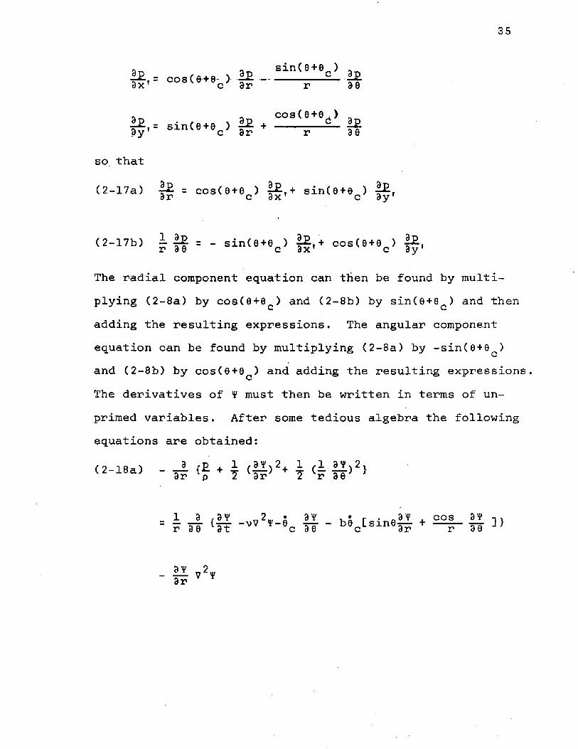
(2-17a) If = cos(e*ec ) ff,+ sin(e+6c ) ff

The radial component equation can then be found by multi­plying (2-8a) by cos(0+0c ) and (2-8b) by sin(0+0c ) and then adding the resulting expressions. The angular component equation can be found by multiplying (2-8a) by -sin(0+0c ) and (2-8b) by cos(0+6c ) and adding the resulting expressions. The derivatives of ¥ must then be written in terms of un­primed variables. After some tedious algebra the following equations are obtained:

The equations to be solved are then (2-13) and (2-18) with boundary conditions (2-16).

(C) Solution of the Linearized Stream Function Equation.For convenient reference the stream function equation

and boundary conditions are rewritten here.

(2-13) (V2y) - Ere + be cose + — ] ^ (v2y)at c c 3r r 30

+ [i - be sine] ^ (v2y) = vV2(72y) r 30 c 3r

Boundary conditions

(2-16a) -0 (a+b cose)c

(2-16b)

(2-16c) ay l ay 3r ’ r 30

The time dependence of the angle 8 is assumed to bev

37

0(2-19a) 0 = -0 cos wt = - -*2- [elwt+ e"1U)t]C o £

030 i . * ,(2«19b) 9 = we sin cut = [ e ^ - e -1® ]c o 2x

A perturbation solution of (2-13) can now be found. The validity of this solution will be discussed in Chapter III. The stream function is assumed to be. of the form

(2-20) V = V + ¥i+ y2+ ■•.0where(2- 21a) -r r (v2f ) = vV2(72'F )31 o o

3Y(2-21b ) 3- 2- ) = -0 (a+b cose)3r r=a c

9 ¥(2- 21c) I TiT W 5cb sin0

9 ¥ 3 V(2- 21d) -sf, i j f . + 0 as r * -

(2-22a) ^ (72^ ) - [reo + beccose+ I l f ] i ^ <v2*o >

3 ¥+ L~ *5— - be sine] — (v2r) = W 2(V24'1) r 30 c 9r o

<2- 22 b > — W 0

3 ¥ 1(2- 22c) i ) = 0r 30 r=a

383 ¥

(2-22d) — i -|f * 0 as r * -

The "zero-order" solution, ¥ , may be found from Eqs. (2-21),the first perturbation, ¥i, from (2-22), etc.

It is desired to have ¥ be a sinusoidal function ofot and 0 . The solution of (2-21) may be found by assuming

(2-23) ¥ = X E xo (r) £Ca s m A 0 + D. cosA0] exp(inu)t)o „ An in AnA = o n= o

+ complex conjugate _

One can find the differential equation satisfied byby substituting (2-23) into C2-21).(2-2*0 <im>- D2} <D2 x*n > = 0

2 2where D a = i Sj--- * • The solution of (2-24) isA , 2 r dr _ 2 dr rfound by assuming

(2-25) xtn(r) = tln(r) +ntn<r>where(2-26a) 0 (n i 0)

(2-26b) {inui- D a}nfl = 0 (n t 0)A An

(2-26c) ❖ *,> = 0 (2-26d) 5j0where Cl is also a solution of (2-26c).AO

The solutions of (2-26a) and (2-26c) are (2-27a) - A tor»+ B ^ p ' * ( M O )

(2-27b) ?on(r) . K on+«onln(r)

39

The solutions of (2-26d) are(2-28a) n = S r 2+ T r 2[ln(r)-l]oo oo ooC 2-28b) m o * s10 rln(r)+T10r 3

C2-28c> ,to = Slor ‘+2* T 4or -‘+2 U » l >Solutions of (2-26b) are Hankel functions of the first

4 2and second kinds with complex arguments•

(2-29) n4n= i»^~n mr) + T £n H^2^(i/nmr) (n t 0)

where m = . The Hankel functions of the first kindvapproach zero as r approaches infinity, while those of the second kind become infinite as r approaches infinity. The boundary conditions then demand T An= 0 for all * and all n £ 0. The time dependence of 0c demands all constants be zero except those for which n=l. By examining the boundary conditions one can see that only a term for which I - 0 and one for which* = 1 (cos6) need be retained.Hence, 't may be written(2-30) y = {[£ + BHCp(imr)] cose + CH(1 )(imr) o r 1 o

+ Dlnr + E) e‘*'U)t+ Complex Conjugate Since E leads to no fluid velocity, E = 0. The term Dlnr may be eliminated, i.e., D = 0 , by the following argu­ment. The terms in (2-3 0) containing cose correspond to the translational motion of the cylinder, while those having no angular dependence correspond to the rotational motion about the center of the cylinder. If no translational

40

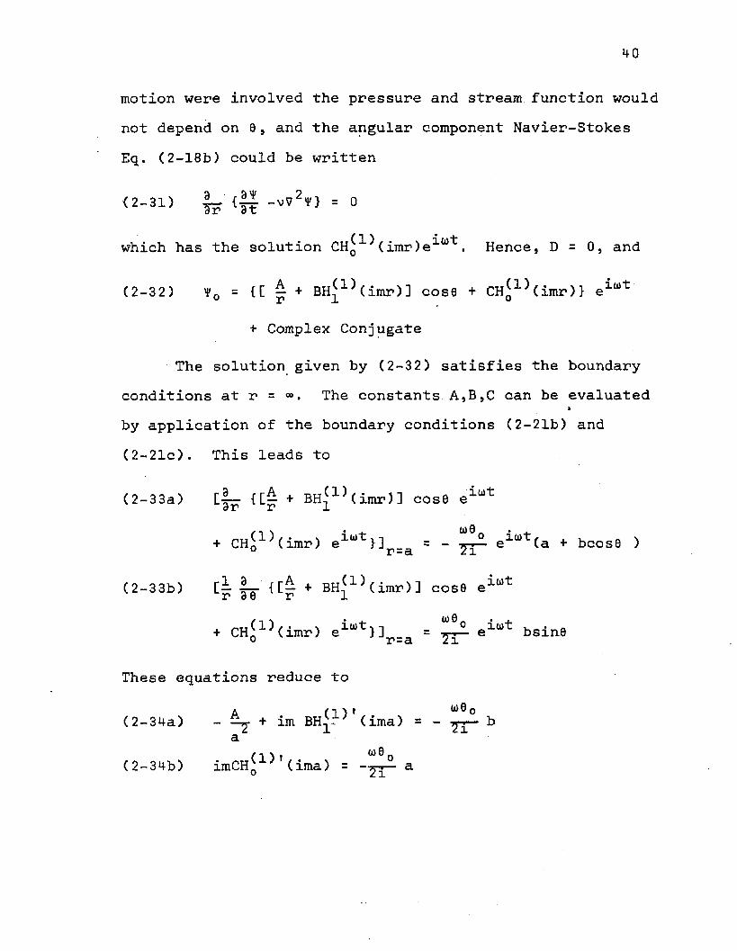
motion were involved the pressure and stream function would not depend on 0 , and the angular component Navier-Stokes Eq. (2-18b) could be written

(2-31) |p -vV2f} = 0

which has the solution C H ^ ^ (i m r . Hence, D = 0, and

(2-32) ¥0 = {[ p + B H ^ C i m r ) ] cose + C H ^ ^ i m r ) } e1(ot

+ Complex Conjugate

The solution given by (2-3 2) satisfies the boundary conditions at r = ®. The constants A,B,C can be evaluated by application of the boundary conditions (2-21b) and (2-21c). This leads to

(2-33a) [|p {[p + B H ^ t i m r ) ] cosG eia)tU) 0

+ CHq1 (imr) elwt}]r=a = - elcot(a + bcose )

(2-33b) {[? + BH^1 ^(imr)] cosG elwt

+ CHq1 (imr) elu)t}]r _a = elwt bsin.6

These equations reduce to

A (11 ? “eo(2-34a) - + im BH£. } (ima) = - ba

( H i o(2-34b) imCHg (ima) = a

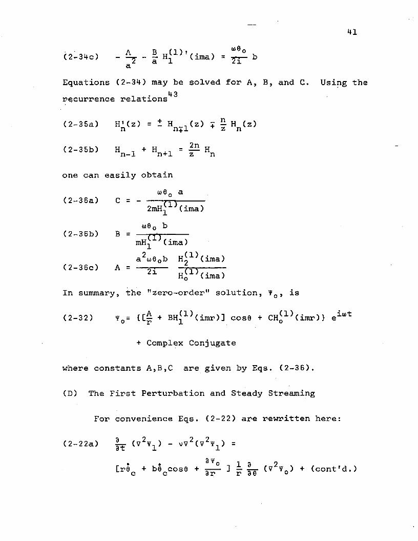
Equations (2-34) may be solved for A, B, and C. Using the43recurrence relations

(2-35a) H'(z) = t H , (z) + J H (z)n n+1 z n

(2-35b) H , + H . = — Hn-1 n+1 z n

one can easily obtain

(2-36a) C = -w 0o a

(2 —36b) B — (1')

2m H ^ ^ (ima)d)0o b

mH^ (ima) a 2u)0ob h!1 (ima)

( 2-3 6c ) A = sq — ri"\------21 Hq (ima)

In summary, the "zero-order" solution, 4^, is

(2-32) 4'0= + BH^1 (imr) ] cos© + C H ^ U m r ) } eltot

+ Complex Conjugate

where constants A,B,C are given by Eqs. (2-36).

(D) The First Perturbation and Steady Streaming

For convenience Eqs. (2-22) are rewritten here:

42

+[becsine- ^ <v‘ vo)

3 ¥C2-22b) ]r=a= 0

1 ” l(2-220) i ^ i ]r=a= 0

3 TC2- 22d) ,-i, i as r -*■ "

When the expression for ¥ , C2-.32) , is substituted intoEq. (2-22a), the following differential equation is

ftobtaxned

(2-37) [|- - v72]724'1 =

2fl tt, * H^^(imr)sinet^ 0 (imbC + B J H ^ C i m r ) + 5— CA — — s----2m *H^1 \ i m r ) H ^2 (-im*r)+ Imw CB*_1__________ 1___________v r

imbw2e m * H^^Cimr)+ Sin 26[— j- 2. BHg (imr)- ^ A B -£---5----

rH1(1 ),(imr)H1(2)(-im*r)

- m. SB J:--------------i__________ ]v r

+ (continued)

* The complex conjugate of H^^(imr) is H^2^(-im*r).

43

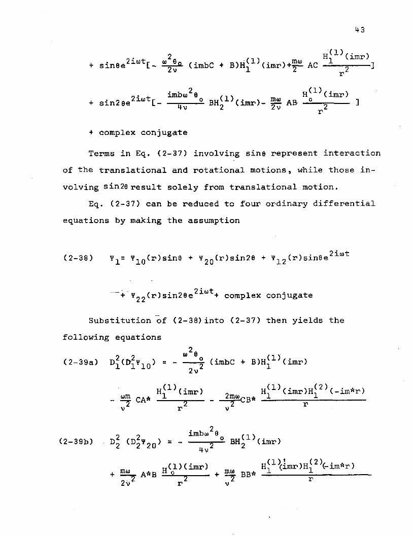
0 . 2a v H ^ ^ ( i m r ’)+ sinQe [- ^^ia. (imbC + B)H^ (imr)+^- AC -— g-----]

«. ^ imbto20 ,+ sin2ee C ^ 2. BH^1 )(imr)- ^ AB -2— ----- ]

r

+ complex conjugate

Terms in Eq. (2-37) involving sine represent interaction of the translational and rotational motions, while those in­volving sin20 result solely from translational motion.

Eq. (2-37) can be reduced to four ordinary differential equations by making the assumption

n * j.(2-38) 4'1Q(r)sine + ¥2q (r )sin28 + ¥1 2 (r)sin0e w

+ Vg2^r )sin20e2lw^+ complex conjugate

Substitution of (2-38)into (2-37) then yields the following equations

20 0 ^ ® n f"lH(2-39a) D^(I>p10) 2. (imbC + B)H^x;(imr)

2v

H n(1)(imr) 0m H1(1)(imr)H1(2)(-im*r)win ri a a iinwpp i J. -L- -y CA* ------J--------z p c B* ------------------------v r v

o o imbd)20 M v(2-39b) D 2 ^ 2 *2 ^ -------BHg (imr )

H (1) (imr) m H1(1 )(imr)H1(2)(-im*r)+ EH— A *B ----- + 2 “ BB* ---------h---------r r A 8 - ^ — 2 + t2v r v

44

2(2-39c) [ 2 ito-v D ^ ] ( D ^ 12) = - (imbC + B)H^1 }(imr)

1 (imr), mw A„ 1 + “ AC ? ----

2(2-39d) [2iw - vD2] ( D ^ 22) = - — ^ V6Q BH^1 (imr)

H (1 )(imr) mu AB o2 v ^ 2r

where(2-40a) D 2 = + I

dr r

(2-40b) T>\ = fliy + i ^ar r

Equations (2-3 9) can be solved using the method of variation of constants. The solution of (2-39a) will beoutlined in some detail. It can be noted from (2-2 9) that(1 ) 2(imr) is an eigenfunction of D^. Hence, ^ q ^ ) can be

written(2-41) I'io (r) = KH(J }(imr) + f(r)

If (2-41) is substituted into (2-39a) the followingresults are obtained

0(2-42) K = —y (imbC + B)

9 9 ™ H ^ ^ i m r )(2-43) Dn [D; f(r)] = - ^ CA* L

0_ 1 ^(imr)HT(-im*r)£1™. CB* — ___________ -_________

The solution of the homogeneous equation

D2 [D2 f^(r)] = 0 is

^2 3f^(r) = C- r + — C3r + C^rlnCr)

The presence of the logarithm makes it convenient to change the variable r to a dimensionless variable,S = — . Equation (2-4 3) may then be written

C2- w c + r ar - [ - t - + r a? " V*f<£)<J{2 5 « 52 de 52= a 4 q ( C )

whereH^^Cimas)

q(l-) = CA* ■ 1 -----v a 5

^22. CB*H^1 }(ima?)H*2 5(-im*a£)

The function, f(£), is then assumed to be of the form

2-45) f u > = e g ^ e ) + j g 2 (c) H 3g 3 (c) + u i n O g ^ . c o

The differential operator in (2-44) may be written r d 2 . I d l - , r d 2 . l d 1

46

If (2-45) is now substituted into (2-44) the following equation may be obtained

j 3 l ^®2 3 d®3 dg4(2"47) u a n + 1 ar- + 5 ■an+cln5 w ]

dgl 1 2 dg3 dg4* ^ C3 a r + 1 ? a r + 55 a r + <31n«+1)a r ]dC

d f3 dgl 1 dg2 13 dg3 (3 31n<- dg4-,+ ar c? a n + tt a n + 135 a n (r i ^ a n - 1

dg3 4 + 16 gji = a ^ c e )

The g(5) functions can be found by setting

dgl . 1 dg2 ,.3 dg3 A dg4(2-48a) 5 + i ^ +«* ^ + «lne ^ = 0

dgl 1 d®2 2 dg3 % dg4(2—48b) 3 ^g**" "j1 t 55 a r - (^inc+i) ar™ ~ ^

,n v 3 dgl . 1 dg2 ^ dg3 , ,3 31ne. dgl» - n<2-t8c> { Jj- + p- g|- + 135 j|- + (? + — 5-) gi- - 0

dg3 4 ( 2-48d) 16 ^2. = a q( C )

Using Kramer's rule one can then easily obtain

dgl E^lnE 4 (2-49a) * a q(C)

47

(2-49b) 231" =

(2-49c) dg3 d£ '

(2-49d) dg4 d£ "

so that(2-50a) g3.CC)

(2-50b) g 2c o

(2-50c) S 3 c c )

(2-50d) g4 C£)

A

16

£2 4V a4q ( 0

x 2lnxq(x)dx + a4 £ 4Yg- x q(x)dx + K2

Yg- f\ q(x)dx + K3Lf

- ■f— x 2q(x)dx +

where the lower limit of integration is chosen as x = 1 so that integration begins at the cylinder surface, r=a.The function, ¥^p(r), may now be found by combining (2-50), (2-45), (2-42), and (2-41)?(2-51a) V1()(r) = (imbC + B) H ^ d m r )

4 £+ ^ [j-— A x 2lnxq(x)dx + K^]

4 £+ ~ C- j g A x 4q(x)dx + K 23

1r

3 4 a+ C IS- lCx)dx + k 3] a 1

4 -+ — In — C- A x 2 q(x)dx + K^]

48

The constants, K^, Kg, Kg, K^, are determined from the boundary conditions. From (2-22) it is apparent that ( r )

must satisfy the following conditions:

10 ^10(2-52a) = -^2.] = 03r r=a r r=a

®^10 ^10 (2-52b) -g-ii, -i2. + o as r + »

The boundary condition at infinity then demands

4 ^ 9(2-53a) K^= - -/^x lnxq(x)dx

4(2-53b) K_ = - r q(x)dxo ± b i

4(2-53c) K^= p-/“x 2q(x)dx

but with three constants determined only one is left to satisfy the boundary conditions at the cylinder surface.The boundary condition at infinity is therefore relaxed

^ 1 0 ^lO(2-54) — r— — , ---- must be finite at r=».3r rWith this condition Eqs. (2-53b) and (2-53c) still hold,

but K- is now undetermined by the condition at infinity.Substitution of (2-51) into (2-52a) then gives the

following results for K^ and K g :

49

0 K(2-55a) Kx= - T p (imbC + B)ima H^1 )(ima)-2K3- -p

6(2 - 5 5 b ) K 2= p {imbC + B) H ^ ^ i m a ) - K p Kg

Equations (2-39b), (2-39c), and (2-39d) are solved in a manner similar to that used in finding . The - -

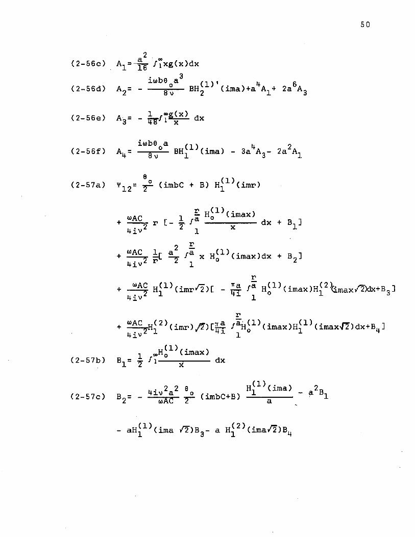
homogeneous solutions used in forming V20 9 *1 2 » *2 2 may be obtained from (2-27), (2-28), and (2-29). Results for 4'20, 1>1 2 , y22 are*

imbe B ,, x (2-56a) Y2Q (r) = — jp2— H 2 (imr)

2 —

+ r 2 C- /a xg(x)dx + A-j]

6 -

+ ~2 fa x 5g(x)dx + A 2]r 1

♦ r 1*: dx + V

“ - ,+ T W x g (x)dx + A 4

„(1),. . (imax)H^(-im*ax)(2-56b) g(x)=£ip- A*B g + 2 “bB-*— --------- -------------

2v a x v

imbe B ,.v*Except for the term — ^ ■"°— H 2 (imr), the functions gCr) and4'22(r)are identical with expressions obtained by Holtsmark, et al., who considered the case of a fixed cylinder in an oscillating stream, with no rotational motion. (See Ref. 25)

50

(2-56c)

(2-56d)

(2-56e)

(2-56f)

(2-57a)

(2-57b)

(2-57c)

2A 1= g<x)dx3ltobQ 3. / \ | j. p

A 2= — BH^ (ima)+a Ax+ 2aDA 3

iwb0 a r-i v 1. nA. = — *— =- BH^ (ima) - 3a A,- 2a A.h 8 v 1 3 1

0'12= y ~ (imbC + B) H^1 ^(imr)

(*»AC 1 ra imax)+ r C- 4 /a ----- ----- dx + B ]4iv^ 1

+ k ^ /a x Hq1 k imax)dx + B ]i+lv2 r ^ ]. 0 2r

+ HlCl)(imr/2)C - ~ /a H^1 k imax )H,( 2 kmax/2)dx+B ]4ivz x 1

r+ H (2 )( i m r ) ^ ) C ^ /aH^1 )(imax)H1(1 )(imax/?)dx+Bu ]

4iv x 1 1, ^ H ^ k i m a x )

V 7 '>-----5------ d*

„ . 2 2 0 Hn(1 )(ima) 2nB2= - T - CimbC+B) “^ - a ---- " 1

- a H ^ k i m a /2)B3- a H^2 >(ima/2)B1+

51

(2-57d)

(2-57e)

( 2-58a)

muAB16v2

mtoAB16v2

(2-58b)

(2-58c)

9 . 2 H (1 )(ima) 2BB _ = — ( imbC+B)— -------- -- 7-rr----- ——3 wAC/2 H (ima/2) im/2H(1} (ima/2)o o

H (2)(ima /2)0 B,

H C1 )(ima/2) 4

B4= - (imax)H^1 ^(imax/2) dx

imbe B (, v V22(r) = ip— Hg (imr)

m ar 9 i T (imax)_ mwAB r 2[ 1 fa _o ---- dx + c -j16 v 4 1 X 1

H £_ A® i_ [» /a x3H (1 )(imax)dx + C«]

16v r 2 4 1 0 22 -

^ 1 )(imr/?) [£f- /a x h£1 }(imax)H^2)(imax/2)dx + Cg]

2 -

d 2)(imr/2>[- /ax H (1) ( i m a x J H ^ (imax/2)dx + Cu]l 41 ^ 0 i. *+

, H (imax)o _ 1 ,°° oCl~ " x dx

2 2U iv a. b0 * ll o 11 \ .C2= ----- Hj (ima)-a a zH^x '(ima/2)C;

- a 2H 22)(ima/2

52

(2-58d) C3(ima/5) 4

lii H f i ma 1

(ima/2)

2(2-58e) ira

4 " Hi

The time independent part of is called the steady streaming and is given by

(2-59) .y = t^gCrJsinQ + V^q (r)sin2e + Complex Conjugate

Both anc* are non_van^s i;i-ng a-t infinity. Thederivatives of ’i'- gSinB are finite at r ~ 00:

(2-60a) {|— C'l'Tnsine3} = — [§— /” x 2lnx q(x)dx + K,]sin6ar xu r -00 a ^ 1

so that the steady streaming velocity components do not vanish at infinity. It is important to note that V ^ s i n e arises from the interaction of the translational and rotational flows. The function 'l’2 0(r,)sin2e results from translational flow only. At infinity V20siri20 and its derivatives behave as follows

= — [77— /" x 2lnx q(x)dx + K, ]cos0 a h 2_ x

(2-6lb) % Ci'20sin2e]}r=„ 0

S3

<2-61C ) {I [f20sin28 ]}r=„ = 0

Hence, if only translational jnotion were involved, the steadystreaming velocity components would vanish at infinity.

In Chapter I the concept of a steady streaming boundarylayer thickness, 6^ , was discussed. In the case of puretranslational oscillations, for low amplitudes is a

1/2function only of a/(v/u>) = a/ 6 (see Fig. 6). Let usnow compare the parametric dependence of 6^ for angular oscillations to that of for pure, translational oscilla­tions.

The steady streaming boundary layer thickness is de­fined as the distance from the cylinder at which the radial component of the streaming velocity (with respect to the cylinder) first vanishes. For the angular oscillating cylin­der the r component of the steady streaming velocity with

1 ^ s srespect to the cylinder is — -g-g— , where

(2-59) ¥ = t1Qsin6 + T2Qs^n20 + Complex Conjugate.

Hence, in order to find for the angular oscillatingcylinder, we set

^10(r> cos0 + 2'1'20(r) cos2e = 0 »

and find the value(s) of r which satisfy the above expression. It is immediately obvious that 6DC for the angular oscillating cylinder is a function of the angle 9.

54

By substituting the expressions for q(x) and the constants C, B, K^, , and into Eq. (2-51) one canwrite Y10 in the form

»10 ■ “ <b6°>2 <F> F(J> jjj^ >jo a # ^where F (— — ) is a complicated function involving Hankel a AC

functions and integrals of Hankel functions. Similarly, from Eqs. (2-56) one can show that can be written in the form

^20 = lo b 0o ^2 *a oAC

Then 6^ satisfies the equation

* F(-^£ a ) cose + 2G(-5£jTS-) cos28 = 0 ,5 a 6AC a 6AC

so that 5£,c/a "the angular oscillating cylinder is afunction of e, a/b , and a / 6 ^ . In the case of pure trans­lational motion the function F would not be present and 6DC/a would then be dependent only upon a /$AC ■

55

(E) Calculation of the PressureThe pressure can be obtained to second order in

amplitude by substituting (2-20) into (2-18):. , a,S 2 . 3 y 2

(2-6 2a) - _ {£ + ^ j I- ] }

3 = F I t - { + '‘'l5 - + V - K T T -

n a 1 ^ 2 T 1 3^0 2<2- 62» +

j\ o o • 3 ¥= - If { le C¥o + V - vV (*o + V - 6c a<r

be Csine 34,° + cose 3¥° 1} 1 3¥° v2v-bec L s m e — + — — - F v

If the expressions for ¥(, and are now substituted into E q s . (2-62) the following equations result:

t n co n 8 r p i 1 r^oi2 , 1 rl 3 To n 2 ■< _ xaiA(2-63a) - _ { t ^ [ _ ] + ? [_ ) = - — y sine e

2+ (im)m*2C C * H ^ (imr )Ho 2 (-im*r) + ^ - B H ^ (imr) C^-

+ im*BH^2 ^’(-im*r)] .+ e2"*- { im^C2H o ^ (imr)H^^ (imr)

+ m 2B H ^ ^ (imr) [ - imBH^'L (imr)] + (cont'd)■ r

56

iu®o a 8v ra** ,a , v, , ,, 2v r ,a 2+ cos9{— 3----- 7r - — r [^r / q(x)dx + K»] - — *-[- -r—- / x q(x)dx2 r 2 a 3 16 1 3 ar2 4 1

+ K^] + im(m*)2CB*H^1 ^(imr)H^2 ^(-im*r) + n^CHo1 ^<imr)[ A*”7r

r 4 £+ cos2e{iu)b90“ - 24vr[f7i /a & -x -dx + A~] + /a x 3g(x)dxo 4 o n X o o X b ir x r x

2+ A^] + (imr) C^* + im*B*H^2 f ( -im*r) ] }

____ 2io»t / i(u9o A ,'wAC Ho1 (imr) W2AC x - H ^ i m a x ) ^+ cose e {--2-----? + JFJ ---- 2----- + 7 7 " l~7 /i- x------dxr r 2v -L

2 2 —+ B,] + iy [ — /a xH^1 )(imax)dx + B ^ + im3CB[H^1 )(imr)]2

2\> r 1

+ m 2CHQ3‘ (imr) [ ^ ” imBH^3" (imr)]}r

2ia)t r . A , mwAB Ho^(imr)+ cos20 e { -lube 0— ---- --------r

imu2AB _ r 1 jr H ^ U m a x ) ^ t „ n imu2ABr „-------r [ r /----- -------- dx + C , J ------T~T~L 24v i x 4v r4 ~ 2

- f- /a x 3H$1 )(imax) dx ] + BH^1} (imr) C^- - imBH^1) ’ (imr) ] }

+ Complex Conjugate

<2- « * > 4 w 4 + + 1 4 ^ ] 2 ) = 0036 e iu t

i^90 A p., t 2 Ho^^(imr)+ sine {-j— ^ ; q<x >dx + k 3 + 111 CA* -2-- j-----

r a 1 r« 4 - „ 0 H (1 )Cimr)HnC2)(-im*r)

- /a x q(x)dx + ] + ni CB* ° ‘ ■ - ~ :---- > +ar d

(cont1d .)

57

TP ( 1 ). ■ - r- A , „„ rl r-a g(x) j i a n i m 2BA* H1 (imr)+ s m 2 6 |iu)b0o— ^ + 24vr[^-g- / — dx + Agj + — --------- ----r 1 r

0 H — o 2„nA. H^A^Cimr.)^ 2 (-im*r), 8v ra „a 3 , , A n , m BB» 1 1 ■,+ T Cl6 f! x g<x>dx + V + — ------------- ?------------- >r xA . n 2iwt / A wAC d r Ho^Cimr) w2AC r D+ sine e { — J 2- - 7T 7 a ? C --- 5 ] " T~T~ [ B1r 2 v

- 1 A H°1)(imax> dx ] ♦ • ! « 1 c«* ,! x „ u > (imax) dx7 1 x -^2~ ^2 2 i

+ B2] + m 2C H o ^ (imr) [ ^ ^ H^^(imr) ]}r x

2 2. „„ 2iuit r • A , ium AB ^d),..___ imui AB „ r ^+ s m 2 e e { - itub90 — g- H1 (imr) + r Lr v *+v

r (!) 9 , r1 a H 0 (imax) imw AB 1 r a ,a . 3U (1),.___ ^+ 77/ dx ] - jj-----5- L —r— f x Ho (imax) dxH 1 x r 1

+ c2l + ^ (imr) [ ^ + | H ^ U m r ) ]}r

+ Complex Conjugate

One can find the pressure by integrating Eqs. (2-63) The two equations serve as a check on the calculation. The pressure is given by

(2-6,) £-12p+- ^ i ! ^ 2 ♦ |[i i ^ ) 2 = -i. t sine eitot2

+ / * ’<- im(m*)2CC*H^1 )(imr) H^2)(-im*r) - S— H ^ d m r )

+ im*BH^2) 1 (-im*r)l - e2lurt [im3C2Hj15(imr) H ^ d m r )

2+ 5^5- H ^ ^ i m r ) ( ^ r (imr)) ] } dr + (cont'd.)

r

58

i 0 4 —+ cos0 {- 0 [5L. /a q(x) dx + K„] + m 2CHo1 ^(imr)[^—A T o Xb I o u Ta x

4 £+ B*H^2^ ^ C-^if x 2q(x)dx + K^]}

+ cos20 {— j— - + 12vr2[^- /a dx + Ag] + ^ Cr 1 r

4 - 2+ /* x 3g(x)dx ] + 5j- BH^1 ^(imr)C ^ + B*H<2 }(-im*r) ]}

, _ _2iuit f lw6° A wAC -_d .-H^Cimr)-, U2AC „ r D+ COS0 e J— - - ^ r ^ L ■ r C B 2

1 Jf H ^ ^ i m a x ) n _ J AC 1 ra 2 _ 0 (1 ) , . _ , D -,— tr f ---- dx 3 + a'■ —* L~7\— / x Ho (imax) dx + B«J

L 1 x 2v 1

+ m 2CHo3' (imr) [ ^ + BH^^(imr) ]}

, _2iwt ( lwb6o A ^ im2wAB (1) , ., imu)2AB „2 r n+ cos2 0 e {-^ j + ~"X 6~v— 1 ^imr' + 5” 1r (i) 9 h r

, 1 ra H 0 (imax) imu AB 1 r a -a 3„(1),. avv .+ t- / dx ] - ---- * jrt-Tr- J x Ho (imax) dx4 1 X S o 2 r> 18 v r'

2+ C 0 ] + 51® Hn(1 )(imr)[ - + BH,(1 )(imr) ]} l 4 l r l

+ Complex Conjugate

Of primary interest here is the pressure at the sur­face of the cylinder, for it is that quantity which will be used to calculate the force exerted on the cylinder. Usingboundary conditions (2-21), Eq. (2-34c), and the relation-. . 44 ship

(2-65) H^1 ) '(ima) = - H ^ ( i m a ) + H^1) (ima),

59

one can obtain, from (2-64),

e 2(2-66) [ ] = - _£ (a2 + b 2 ) - sine ei“tp t a

02 ia)0o a 8vK~ 2vKu aba>0 9 n x+ cos0 {ab -p— + — — + — 2~ ~ — 2“ + — m CH° tim a ^

a clitob0o . 9 j, abw0 9 fi }

+ cos20{— ^ ^ + 12va Ag + \ + — ^ m BHj1 (ima)}a a

, oose 2i(dt | + »A£ + lmH<l>(ima)]2 a 2iv a 12 ab(o60 a /-i \

+ I— - aB ] m 2CHo (ima)}2v a 1 2x

2ia)t r ltobeo A A im2u>AB „u(l> / N+ cos29 6 { "g"'""" — ^ ■*" ^ 6v (ima)a

• 2 * n a Cn ab(o6 a / 1 \+ imm AB L a 2c _ _2 ] ---- ^ m 2BH<1 }(ima)8 v a

+ Complex Conjugate

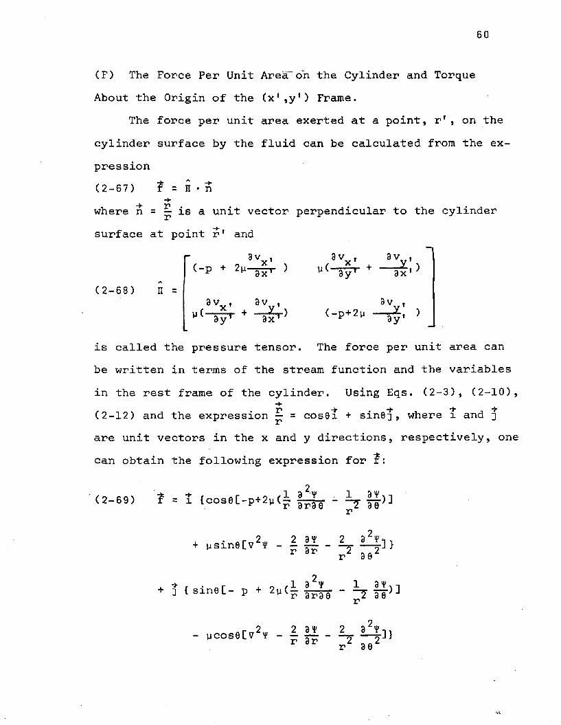
(F) The Force Per Unit Area- oh the Cylinder and TorqueAbout the Origin of the (x',y') Frame.

The force per unit area exerted at a point, r 1, on thecylinder surface by the fluid can be calculated from the ex­pression(2-67) ? = n • n

where n = ^ is a unit vector perpendicular to the cylinder surface at point r 1 and

is called the pressure tensor. The force per unit area can be written in terms of the stream function and the variables in the rest frame of the cylinder. Using Eqs. (2-3), (2-10),

are unit vectors in the x and y directions, respectively, one

(-p + )9v .

( 2 - 6 8 ) n

(2-12) and the expression — = cos0x + sine^, where l and 3

can obtain the following expression for ?:

61

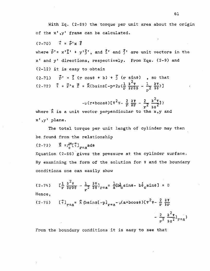
With Eq. (2-6 9) the torque per unit area about the origin of the x',y' frame can be calculated.

(2-70) t = r 1x ?

where r ’= x '!1 + y']f, and i' and are unit vectors in thex' and y 1 directions, respectively. From Eqs. (2-9) and (2-12) it is easy to obtain(2-71) r' = l (r cose + b) + j (r sine) , so that

2(2-72) t = r'x ? = &{bsine[-p+2y (^ ]

r

-y(r+bcos6)[72¥- 1 |X - 1, — *■] >r r ee

where k is a unit vector perpendicular to the x,y and x',y' plane.

The total torque per unit length of cylinder may thenbe. found from the relationship(2-73) j& =/21T[t] ade o r=aEquation (2-66) gives the pressure at the cylinder surface.By examining the form of the solution for ¥ and the boundary conditions one can easily show

(2-” > U w - 7 H w l y s i n e - beoBine] . 0Hence,(2-75) tT]r_a= £ {bsineC-pl^.^ufa+bcose):?2'*'- | ~

- 2- ill] }r 2 3 02 r=a

From the boundary conditions it is easy to see that

62

z o n c \ r 2 3 ¥ 2 3 ¥-| _ 2(000 ~ n o " t „„„4 .-4__(2-7 6) L- — -s— - — 77 — • yJ„. - — 0 *a e + complex conjugater 3r r 30 a

2An expression for [7 I'D can be obtained from Eqs. (2-32),(2-38), (2-56), (2-57), and (2-58). When that expression is combined with Eq. (2-7 6) the following equation results:

(2-77) [V2¥- 2 i ! - i-I] = m 2BH^1 )(ima)cos0e1“tr 3r r 2 3 0 r=a 1

j. r™2r,1J(l)/ - ^ 2(o6o i „i(ot+ Lm Crl (ima) + —**-»—• j e0 z x

0 9 r i 8K~ 2KU+ sin0{y2. [imbC+B]m H, (ima) + — g-- + -a--}a a

im^b© ,, . 9 4AU+ sin20 {----q— 2- BH^ (ima) + 12a^A3---

cl(1)

0 . . 0 o / i \ a n H m a )+ sin0e {- ^2-[imbC+B]m h| (ima)-------- -2-^------2iv‘

10AC 2rB2 , „- --- 77 m [— + aB, ]}2i\> a 1

+ sin20e2iwt {- B H ^ ^ i m a ) - E£*AB H ^ U m a )8v 0

+ 5X2^£[^| + a 2e ]}8v a

+ complex conjugate.-By examining Eqs. (2-73)and (2-75) one can see that only

that part of the pressure which contains sin0 will contribute22 234* 2 3 tto the torque, and only those parts of (V ¥- — ^

which contain cos0 or are independent of 9 will contribute.

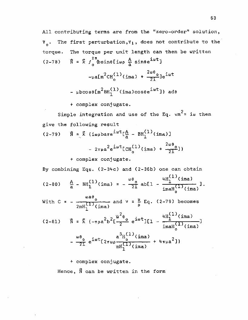
63

All contributing terms are from the "zero-order" solution,4* . The first perturbation,¥i , does not contribute to thetorque. The torque per unit length can then be written(2-78) ft = 5c /2T{bsin0[io>p - sin0ela)t]o a

r 2_„(1 ) . . . , 2a)0on ioot-ya[m CHq (ima) + Je

- ybcos0 [m^BH^^ (ima^osOe'*'^] } ad0

+ complex conjugate.2Simple integration and use of the Eq. vm = io) then

give the following result(2-79) ft = ft {i(i)pbairelu)t[— - BH,( 15 (ima) ]3. X

- 2irya2ela,t[CH(1 )(ima) + -^-2-]} o 11+ complex conjugate.

By combining Eqs. (2-34c) and (2-36b) one can obtainA ,, o)0 (ima)

(2-80) - - BH^---(ima) = ----*5- abCl - — n v ].a 1 21 imaH C ima)0

(ua0With C = -----

2mHJJ d O7. .°---- and v = — Eq. (2-7 9) becomesn (ima) P

_ o o w 20 . + 4Ha1 }(ima)(2-81) N = k {-upa b C-^-2. ela)t] [ l n s------]

imaH (ima) o0)0 . . a^H^^(ima) 0

- — ela) C2tto)p— ------- + 4irya ]}mH, (ima)

+ complex conjugate.Hence, ft can be written in the form

64

* 2 2 2 “tH^'cima)(2-82) N = - ku> 0 coswt {irpa b [1-Re( t-s-t------ )]0 imaH (ima)o~ H (ima)

+ 2irpa Im[-°-ry .------ ]}mH^ (ima)

+ 2 2 (ima)- ko)0 sinujt{Trpa b wlm[ ppc------]0 imaHo (ima)3 (ima) 2

+ 2iTpa wReC— t-t-?------ ] + 4irpa v}mH-^ ( ima)

2 2In Eq. (2-82),irpa b =1' is the moment of inertia (per unit length of cylinder) of the fluid displaced by the cylinder. The parameters k and k ’ are thus defined by the equation

(2-83) ft = - ic{I'kec+ I'k'ue }so that j •* . * -i \

4H-, (ima) 2 H^x;(ima)( 2-84a) k = 1 - ReC- _--] + 2 ImC (I)'.----~]

imaH (ima) b maH, (ima)o 1U H ^ ^ i m a ) 2 H (1 )(ima) u

(2-84b) k 1 = ImC 1 + Re[ ° m + ^ TimaH (ima) b maH, (ima) tobo 1In Eq. (2-84a), the terms

4Hj1 )(ima)1 - Re[ ------] are the contributions to k caused by

imaH0 (ima) translational motion, while

2 2 H (1 )(ima)— ImC— 2— ----- ] is the contribution caused by rotation.b maH ( ima)

4h 5■*" (ima)In (2-84b) the term ImC ------3 represents the contri-

imaH (ima)obution of translational motion to k 1, while the other two terms may be attributed to rotation.

65

The argument of the Hankel functions in Eqs. (2-84) is ima = ^ C-l+i). For large values of the Hankel functionsA A

4 5can be expressed m the form of asymptotic series, and k and k T can then be expressed as power series in . Foralarge values of

oc \ 4H1 (ima) 2A A3 r 2 A A2 A3-,( 2 - 8 5a) --------- m -------------- = - g- + I C ™ + ~ n r -- g-]imaH (ima) a 8a d a a 8a doH (1 )(ima) . .2 „ .3 . q .3

(2_85b) H (l)f . 7 ~ 7a " ~ 2 + 32" “ 5" +~ 1 *-2a 32 ~ 3maH^ (ima) 4a a a

Eqs. (2-84) may then be written,

(2-86a ) k = 1 + + —— g- + %-C^- - Lr ig.)a s P b2 a ^ a 3

,2 .3 2 - 2 ^ ^ 3(2-8 6b) k' = g- + (E + + TF ^a 8a b 2a a

2The terms having — *■ as coefficient represent the rotational

bcontributions. The remaining terms result from translational motion and are identical with the expressions found by Stokes^ (see Eqs. (1-5))'. It is apparent that the rotational terms are negligible for a<<b.

The results of the perturbation solution may be summarized as follows:1. The effects of rotational motion upon the low amplitude period and damping parameters are negligible for a<<b.Exact expressions for k •and k* are given in Eqs. (2-84) and (2- 86).

66

2. The streamlines of the steady streaming for angular oscillations are given by Eqs. (2-51), (2-56), and (2-59). Interaction of the rotational and translational motions introduces a difficulty with the boundary condition at infinity.3. Expressions for the pressure and viscous forces obtained from the perturbation solution are given by Eqs. (2-66) and (2-77).*4. The steady streaming as well as all other second order terms have no effect on the torque caused by the force exerted on the cylinder by the fluid.

CHAPTER III SEPARATION MODELS

It would be desirable to find an exact solution of the stream function equation for the high amplitude oscillations of a cylinder in an infinite fluid. One could presumably explain the high amplitude experimental results for k and k' with such a solution. By examining the stream function equation, however, one can see that exact solutions of that equation are not easily obtained.

Although the exact features of the fluid flow must be found from the exact solution of the stream function equa­tion, it is possible to form a "model11 in which the expected gross features of the flow are contained. It was shown in Chapter I that separation probably occurs during the high amplitude oscillations and that separation has a pronounced effect upon the force exerted on the cylinder by the fluid.A model of the fluid flow at high amplitudes must therefore include separation. It would be hoped that a quantitative description of the force at high amplitudes could be ob­tained from a model which included separation.

In this chapter two models based on the occurrence of separation will be presented: (A) a potential flow modeland (B) a viscous flow model. In order to simplify the problem, the rotational motion discussed in Chapter II will be neglected. The effects of the rotational motion should be small compared to those of the translational motion if

67

68

a<<b. The cylinder motion will be assumed to be a sinusoidal translational oscillation along the y' axis of an inertial reference frame; the origin of that reference frame is assumed to be the equilibrium position of the cylinder. (See Fig. 10).

The amplitude of oscillation will be assumed to liebetween the critical amplitude found by Kimball (Ac = »/Ta)and an amplitude of about 2.5 times the cylinder radius, a.Recall (from Chapter I) that the minima in Kimball's Akcurves occurred at an amplitude of about 2.5 a, and thatKeulegan and Carpenter observed that the minimum in theirinertia coefficient (C ) curves occurred when a single vor-mtex was shed (at a relative amplitude of about H.8 ). It is then possible that vortex shedding may also be related to the minima in Kimball's Ak curves. The assumption that the amplitude lies between /Ta and 2.5 a then (hopefully) ensures that vortex shedding does not occur. In this amplitude range the separation process is in its early stages of development.

The flow pattern is divided into two regions: the sep­aration region (i.e., the region enclosed by the streamline attached to the points of separation) and the region outside the separation region. The fluid is assumed to be infinite in extent. In Fig. 10 the x',y' axes are axes of an inertial reference frame, and the x,y axes are axes in the rest frame of the cylinder. The position of the center of the cylinder relative to the origin of the x' ,y' axes is denoted by yc ; the velocity of the cylinder is y and the cylinder

69

SEPARATIONREGION

'fig. 10. Notation for Cylinder Performing Linear Translational Oscillations

As the cylinder is moving upward, the separation region is symmetric about

i Q6 = yi . The x 1 ,y f axes are axes of an inertial reference frame, and the x,y axes are axes in the rest frame of the cylinder.

70

acceleration y . The separation angle 6 is measured from c sthe -y axis while the cylinder is moving in the + y ’ direction and from the +y axis while it moves in the oppo­site direction.

The assumptions made for the separation region and the basis for each are the following:1. Separation occurs when the cylinder has moved a distance /Xa from a position of rest. This assumption follows directly from Kimball’s empirical critical amplitude rela­tionship *'Ta.2. The separation angle 8 is zero at the start of separa-stion. During a half cycle, while the cylinder passes from one position of rest to another, 0 increases rapidly fromozero at first, reaches a maximum, and then decreases back to zero in approximately the same manner in which it first increased. The assumed behavior of the separation angle is based upon the behavior of the separation angle in the examples of separation in fluid flow about cylinders dis­cussed in Chapter I. Since the cylinder motion is a sinu­soidal oscillation and the amplitude is assumed to be less than that required for vortex shedding, the separation angle should begin at zero and return to zero during a half cycle.3. In the amplitude range of interest the fluid velocity (relative to the cylinder surface) in the separation region is expected to be small. This also follows from the dis­cussion of separation in Chapter I. It is assumed,

71

therefore, that in the separation region the fluid near the surface of the cylinder moves with the same velocity as the cylinder.4. The pressure is continuous at the points of separation. The streamline joining the points of separation can at worst develop into a vortex sheet. It is well known that the pressure is continuous across a vortex sheet.

The other physical assumption that needs to be made is that of the flow pattern outside the separation region. The two models that are presented in this chapter differ only in that assumption. The quantitative features of the models can now be presented.(A) Potential Flow Separation Model.

The simplest assumption that can be made for the flow outside the separation region is that the flow is inviscid potential flow about the cylinder. The fluid velocity in the nonseparated region is then derivable from a potential function, <J>:(3-1) v = -V'*where v is the fluid velocity in the x*,yf frame.

-*■ 2Since the fluid is incompressible, V»v = V <j> = 0.The boundary conditions are that at the cylinder surface the fluid velocity component normal to the cylinder surface is equal to the component of the cylinder velocity in the samedirection, and that the fluid velocity must vanish at infi­nite distances from the cylinder surface.

72

The component of the cylinder velocity perpendicular to the cylinder surface is y sin9, where 0 is the angleLmeasured from the x axis. The fluid velocity component normal to the surface is vx ,cos6 + vyIsin0 =

- cos0 - sin0 . The boundary conditions are bestexpressed in the x,y frame. The coordinate transformation from the x',y' frame to the x,y frame is accomplished by the following equations:(3-2a) x = x'(3-2b) y = y ’-yso that (3-3a)(3-3b)

3 _ 33x,_ 3x 3 33y'“ 3y

(3-3c) = |^]x#y - yc

From (3-3a) and (3-3b) it is then easy to obtain

(3-4) vx ,cos0 + vyfsin0 = - ~ cos0 - sin© =-|~and(3-5) 7 |2<fr = V2 = 0

The function <J> then satisfies Eq. (3-5) with boundary conditions

C3-6a) - ||]r,=a= yc sine

C3-6b) i | | + 0 a s r - » «

The potential function is readily found to be2

(3-7) <j> = y — sin0T ^c r

73

The pressure can be found from Eq. (2-la), which may be written for potential flow in the x,y frame in the follow­ing manner:

(3-_8 > i f + *<T > * - 7and since v = -V$,

( 3 - 9 ) V [ - | ± ♦ ♦ £ ] = 0

Hence,/ 3_n Q s P"PQ _ 11 _ * _ <Zi>ip 3t 3y 2where p is the pressure at r=«». At the cylinder surfacethe pressure is 2

2(3-11) (P“P 0)r=a = pa^c sin0-pyc cos20~ £~T~

In the separation region the fluid near the cylinder surface moves with the same velocity as the cylinder, and the fluid velocity can be obtained from a potential function,

= -y_r sin6. The pressure at the cylinder surface in thes cseparation region is easily found to be

. 2p-p y(3-12) C— -— -aycsin0+ —|— + T(t)

where T(t) is a function of time which is added so that the pressure will be continuous at the points of separation

(0 = ?jr- - 6g and 0 = + 0S )* The function T(t) may befound by equating the pressure in Eqs. (3-11) and (3-12) at either point of separation. This procedure yields

74

• 2 2(3-13) T(t) = - 2ay cos6 +y cos20 - y , so that the pressurec s o s oin the separation region becomes „

P-Po .. .2 *c(3-14) [— -— ] = -y.a(sine + 2cos8 )+y cos2e - ■*—P r — a C S C S fc

The force per unit length of the cylinder opposing the cylinder motion is

2ir(3-15) F = - /opsineade,

and this force can be written as the sum of the contributions of the separation region and the non-separated region.

3 iry-+9(3-16) F = p/ s[ay (sin0+2cos0 )- y cos2e ]sin0adeo J c s c sli-fl~ 9s

3ir fl o _2 ~ s „ . 2 + p/ Q +/ [-yca sin8+ yccos20]sin8ad0° il+fl~ +0s

The integrals are easily performed to give20_ sin20

(3-17) F = pa{-ira y [1 -C TT IT

2y^[i sin30 - sin0 ]}.C O s sIn the amplitude range of interest the separation angle

is expected to be somewhat less than 90°. The dominantterms in Eq. (3-17) may then be found by retaining only the

3terms up to 0s in the expansions of the sine functions inpowers of 0 . This procedure,which will be examined later, sleads to __

75

irpa is the mass (per unit length of cylinder) offluid displaced by the cylinder.

Let us now assume that at t=o the cylinder is at a restposition a distance A below the x' axis. The origin of thex 1,y' is the equilibrium position of the cylinder. It isassumed that separation does not occur until the cylinder has

1/2moved a distance (Aa) . Then up to the time t that sepa­ration begins, the separation angle 6 is zero, and the forcesexerted on the cylinder by the fluid is given by (3-19) F = -M'yc

The equation of motion of the cylinder is then (3-20) Myc+ 1+ir otyc= -M’ycwhere M is the mass (per unit length) of the cylinder and

24 it ayc is the linear restoring force. We assume M>>M' so that the first approximation of the function yc (t) is (3-21) y = -A cosuit

22where A is the amplitude and ui = — .1/ 2After the cylinder has moved a distance (Aa)

separation begins. At the initial separation time, t ,s(3-22) - A cosurtg + A = (Aa)1/2so that

(3-23b) sinwt(3-23a) cosuit

ss

TP" T 1A A

76

During separation the force is given by Eq. (3-18). Inorder to use that force one must know the time dependence of6 . The separation angle is expected to begin at zero and sreturn to zero before the end of a half cycle. It is assumed

*TThere that separation occurs for a time — - 2tg during eachhalf cycle. The separation angle is assumed to be periodic

2 at gand depend on the function sin w (t-t ) , where w = <jj/(1— -— ).S S 5 «3Since only terms containing 0 appear in Eq. (3-18), a simples

assumption for the time behavior of 0s is

(3-23) 0 = (G sinw (t-t ) } ^ ^s s swhere G is some function of amplitude, cylinder radius, andpenetration depth. The assumed time behavior of 6s is seento have the property of increasing rapidly from zero, reach-

1/3ing a maximum of G , and decreasing to zero in the same manner in which it initially increased. The assumed be­havior of 0 is well in accord with the physical assumptionss

1/3discussed earlier in the chapter. A plot of 0S/G is shown in Fig. 11.

The equation of motion of the cylinder during separa­tion then has the form

(3-24) Myc + 4n2ayc = -M1yc {1 - y| sinwg (t-tg ) }

“ TiF 6 sinoj (t-t )3 it a s sUsing the first approximation of given by Eq. (3-21)we then obtain(3-2 5) My + 4 ir2 ocy = -M’w2Acoswt + MK,coswt sinw (t-t )

J C J C 1 s s+ MKoSinw (t-t ) + MKucos2wt sinw (t-t )0 S S 4 S S

77

1/3

- 1.0

-0.5

Fig. 11. Assumed Time Dependence of the Separation Angle

78

where,o v - M ' 4G 2a( 3-26a) K-, - ry ■ y lL) A'1 M 3 TTtQ V - HG 2 A 2(3-26b) K 3= - ^ tt —

{-> V M* *+G 2 A 2(3-26c) K, = n— -■=— a) ——4 M 3tt a

In the Appendix tiie expressions for Ak andak’ resulting from a force of the form on the right hand side of Eq. (3-25) are derived. From Eqs. (A-27a) and (A-27b) we obtain

(3-27a) Ak’= sinwt {- —7 ^ a s “ t t i

2(0

. ir 1 I - ,+ ttL --------- o - itJ1 03~ 03 * 03s 0l£3 + 4 ^ + _ “ 3_4-£+^JL

oi 2 03 2(0 03

WQ U)Rcos2a)t (1— ) (1+— )S r U W -1 ,T 2 2 ?

3 - 4 ^ + ^ 3 + 4 ^ +^03 2 03 20) 03

Ws 2 ws 2on ( 1 +—■—CO S lilt ) (1— =COS »t )(3-27b) Ak = - 8G c “ _ .JL_ +- 2------ « ]3rr „ s.^l s <*>!

2 ~ +“T w------2(0 0)

2uts /lawhere u = w/[l - ---- ] and coswt = 1 - — y—s tt s A

In order to proceed further we must assume some value for G. It has been found that the simple assumption

AG-K-:— > where K is a constant (independent of A,A , and a), /Aa

79

makes the agreement between theoretical and experimental values of A k 1 very good.

15Experimental values of Ak' (obtained by Kimball ) forseveral fluids and two different cylinder radii are plottedversus theoretical values of Ak'/K in Fig. 12. From theslope of the straight line we find K « 0.16, so thatG = 0.16 A//xa and 6s = [0.16 sinws(t-ts >]1/3. In Fig. 12A//Xa ranges from about 1 to 6 . A value of A//la = 6 givesa maximum separation angle of the order of 1 radian. Itwill be recalled that in passing from Eq. (3-17) to Eq. (3-18)we expanded the functions [j sin30g - sin0g] and[-20 + sin20 ] in powers of 0 and retained only terms in s s s30 . At the higher values of A//la it is seen that the higher s

order terms in the expansions will offer significant contri­butions, although the dominant terms are still those con-

3taining 0 . However, for the experimental data shown inFig. 12, when A//Xa >5 the relative amplitudes, A/a, aregreater than 2. Vortex formation is probably occurring atthose high relative amplitudes and the entire theoreticalapproach is probably invalid. The calculations of Ak and Ak'become very complicated when the higher powers of 0 areretained because those higher powers then introducefractional powers of sinw (t-t ) into Eq. (3-25).s s

With G = 0.16 A//xa the parameter Ak can be determined.. Since coswts and ws/w are dependent only upon A//Xa, the expression for Ak given by Eq. (3-27b) is also dependent

0.8-

0.4-

Ak' (EXP.)

/

° / / a .

/

/ */ 5.8

5.2

A //

v / #A / A

■ / °i /

mt A

/A ■ /, / °< n CC(4

ISOPROPYL H20 ALCOHOL

0.64 CM 0.32CM A

▲

t = 4.4 SEC.

A k '/K (POTENTIAL FLOW MODEL)

Fig, 12. Experimental Values of Ak' vs. Potential Flow Model Values of Ak'/KA . . . A(Values of -tt— are given for the experimental points for which -tt— >5)/A3. r Ad

ooo

81

only upon A//xa. The theoretical values of Ak are compared with Kimball’s experimental results in Fig. 13, where ^is plotted versus A / A a . The theory predicts a decrease in Ak which is much too small. However, the experimental values of Ak also apparently depend only upon A//Ia.

By examining Fig. 13 one might think that with a different choice of K the theoretical Ak curve could be made to agree with the experimental data. However, the value of K chosen would have to be about 1.6, which is ten times the value chosen for the Ak’ curves. The value of 1.6 leads to maximum separation angles which are greater than tt/2 even for A//\a as small as 2. The chosen value K = 0.16 leads to very realistic values of the maximum separation angle.

(B) Viscous Flow Separation Model

In the potential flow model the viscosity of the fluid was neglected. In this section the results of Chapter II will be used in an attempt to include the effects of viscosity.The purpose of this calculation will be to see if the inclu­sion of the viscous terms leads to a better explanation of the experimental Ak results.

For a cylinder performing translational sinusoidal oscillations along the y' axis (see Fig. IQ), the stream function equation may be written in the form

(3-28) (V2?) + [i |1 - y„sine] f- (V2*)3t r 30 J c 3r3V . . Q n 1 33F + yo=°s« 3 F 38- C It * y„c°se ] It <v2,,) = v72 (72f)

82

a O

0.2POTENTIAL— FLOW MODEL

- - 0,6

Ak- - 1.0

-- 1.4

ISOPROPYL CCL ALCOHOL

0.64CM. 0.32 CM.

t * 4.4SEC.

542 3

Fig. 13. Comparison of Experimental and Potential FlowAModel Values of — — Ak/Aa

where r and 6 are cylindrical coordinates in the rest frame of the cylinder. Equation (3-28) follows directly from Eq. (2-13). The boundary conditions are (3-29a> H ] r=a= - ycc°se

C3-29b) i h sin0A dimensional analysis of the stream function equation im­plies that the prime criterion for the application of a per­turbation method of solution is that the relative amplitude,

2 6A/a, be small compared to unity. However, the solution of Eq. (3-28) is not known for high relative amplitudes. It is assumed, therefore, that the flow near the cylinder surface and outside the separation region can be approximated by the solution obtained by the perturbation method used in Chapter

The second order (in amplitude) solution of Eq. (3-28) can be obtained directly from Eqs. (2-32), (2-36), (2-56), and (2-58). The only difference between the solutions of Eqs. (3-28) and (2-13) is that the rotational terms are omitted in the solution of (3-28).

The force per unit area has the same form as that appearing in Eq. (2-69). The force per unit area opposing the cylinder motion is

84

The pressure can be obtained from Eq. (2-66) by omitting rotational terms from that equation and replacing b 0Q by the amplitude A.* The pressure may be written in the form

(3-31) i $1 + Qosin0eiut

+ Q 2 q C O s 26 + Q 2 2 c o s 2 0 e ^ 1(ot

where+ complex conjugate

(3-32a) Q = -xo aL\i A

to O O V. rs ill) A E , - i o 2. . 4 , a (I) A 2 nu (1) / • \(3 — 32b) Q20- ” 2— ~*2" 12va + g^ m (ima}a a

( 3-32c) Q 22 = % + a H ^ ^ i m a )a

, imio2EB r - C 2n au>A „2DU(1),„._ ,+ --- -- La C- — — j-J - g-£— m lima;8 v a

(3-3 2d) m 2 = —v

2 A (ima)(3-3 2e) E = ---- [from (2-36c)]

1 Ho (ima)

(3-32f) B = tn \ A [from (2-36b)]mH (ima)0

* The constant, A, appearing in Eq. (2-66) and given by Eq. (2-36c) will be denoted here by "E" in order to avoid confusion with the amplitude, A.

85

(3-3 2g) Ag= - ■ig-/7^r^cix [from (2-56)]

H \ imax) h5 \imax) h5 2 \-(3-32h) g (x ) = 5^- E*B ° j -~2----- + BB*— --------— i--

2v a x v

( 3-32i) A, = BHnCl)(ima)-3a4A„-2a2A n4 8v 1 3 12

(3-32j ) A± = Ye/7xg(x)dx

, H (imax)(3-32k) C1= - £/7~ — £ dx [from (2-58)]

(3-321) C2= H^1 )(ima)-a4C1-a2C3H^1 )(ima/2")

- a 2C1+H 22 )(ima/2')

-4aC, H-5 2 (ima/5")(3-32m) C~ = -— -------------- f-n--------- Cu

im V ^ J (ima/2-) (ima/2 ) 4

2. Hn(1 )(ima)+ ^lv A 1 _______toE/2 (ima/T)

2(3-32n) C4= fix H ^1 (imax)!^1 (imax/T) dx

/o a,.N rl 32V 1 3»n _ nFrom Eq. (2-74), I- - -y T ? ]r=a= 0,r

and from Eq. (2-77),

(3.33, [, V | g - ^ i!|W B.co...1"*

im*ax)

n •+ R 2Qsin2e+ R 22sin20e w + complex conjugate

86

where(3-34a) R 0 = m 2BH^1 )(ima)

3 a n } ? 4Au(3-34b) R20- im £ BHj (ima) + 12a Ag-a

(3-34c) R2 2 = -im3 ^ BH^^Cima) - mw— 2^'*' (ima)8 v '

, 3 EB r C2 . 2n n+ m iO ■ y L— y * cL C-, J8v a x

Equations (3-30), (3-31), and (3-33) may be readily com­bined to give

(3-35) f = - sin0{p - ~ py2 + [pQ sin9e^'u't* 0 £ C 0^ • i

+ P Q2 oc°s2 0+pQ22c o s 2 0 e u + C.C.]}

* i-ycos0 (RocosOe140 +R2osin28

ft ' x+R22sin20e +C.C.HC.C. =complex conjugate)

Equation (3-35) gives the force per unit area opposing the cylinder motion in the non-separated region. The force per unit length of cylinder caused by the non-separated region is given by

3i . 02 s(3-36) F = S +/- f a d0n 0 d7T + fl3~+0s

Substitution of (3-35) into (3-36) and subsequent integration yields

(3-37) Fn= -2asin0s[po- j py2] -pa{ (^e1U)t[Tr-0s- ^ sin20g]

87

(3-37) + Q2 oC-sin6 - i sin30 ] + Q2 2e^ a)tE-sin0 - isin30 ]S o S S o S

+ vRoe^a,t[ir-0 + i sin20 ] +vR2 oCsin0 - isin30 ]S Z 5 S O S

+vR2 2e^1U)ttsin0 - isin30 ] + complex conjugate}S o Swhere v= p/p .

In the separation region only the pressure contributesto the force. The pressure in the separation region hasthe same form as that given by Eq^ (3-12):(3-38) [ --- -] = - ay sine + — + T(t)p r=a J c 2

where the function T(t) ensures continuity of the pressureat the two points of separation. Once again T(t) may befound by equating the pressures in Eqs. (3-31) and (3-38) ateither 0= -0 or -1 - +0 . T(t) is found to be2 s 2 s(3-39) T (t ) = -ay cos6 - y^-(Qo cosB e ^c s c s

+ Q2 ocos20 +Q22cos20 e2iwt+ C.C.}, s sso that the pressure in the separation region is given by

1 • 2 ** ••(3-40) plr=a= P0“ -Z°yc - aycpsine-payGcos ©s

-p {Q0cos8 „ela)t+Q2 ocos2 0 s s

+Q22COS20 e2iwt+ C.C.}OThe force per unit length of cylinder caused by the separation region is

3jL+e(3-41) Fg = / 2 s[-p]r>_asine ad0

88

Substitution of Eq. (3-40) into (3-41) and integration gives

(3-42) F = 2asin0 [p - ipy^]-ap {-ay*[0 + \ sin20 ] s s o c c s s

-ay cos0o[-2sin0_] + [2Qoellotsin0 cos0_O S s S o ­rt •

+2Q2osin6_cos20 +2Q22e W sine cos2e s s s s

+ complex conjugate]}The total force per unit length opposing the cylinder

motion is the sum Fn+ Fg . Use of simple trigonometric iden­tities in Eq. (3-42) and addition of the expressions in (3-42)and (3-37) gives(3-43) F = F + F = - aptay ( i sin20 -6 )] s n — • c s s

- ap{irela)t(Q0+vR0) + (Qo + v R o 7 sin2es~es]

+ [2Q2o-vR2o]Cjsin30s-sin0s]

+ [2Q22-vR22]e2;La)t[i-sin30 ~sin0 ] + C.C.}o s sOnce again we expand the sine functions in powers of 0S and

3retain only terms in 6 . Thxs procedure yields _ s

(3-44) F = 7TPa ^(yc' '0g) _aP {,re^U)t[Qo + vRvo]

- gf2Q2o_vR 2o3

- -j 0gC2Q22j-vR22e2la>t+ C.C.}3 #• 2 2Letting 0 = Gsinw (t-t ) ,y = w Acostot, and M'=Tipa , we cans s s o

write Eq. (3-44) in the form

89

(3-45) F = - M'w2k Acoswt - M'w2k'Asinwto o

+ MK, coswt sinw (t-t ) + MK,*sinwt sinw (t-t )1 s s 2 s s

+ MK„ sinw (t-t ) + MK(1c o s 2 w t sinw (t-t )3 s s 4 s s

+ MK sin2wt sinw (t-t ) s s swhere M is the mass (per unit length) of the cylinder, and

(3-46a) k = - J — RE(Q0 + vR0)o z . w Aa

(3-46b) k' = --- \-- IM(Qq + vRq)w Aa

(3-46c) = jjj— w2A(^-) + RE(Q0 + vR 0)

M 1 UG(3-46d) K2 = - ^ IM(Q0 + vR0)

(3-46e) K S * g l l f j RE(2Q20-vR20)

(3-46F) K* = ||^ RE(2Q22-vR22)

(3-46g) K 5 = - IM( 2Q22-vR22 )

The Q's and R's are given by Eqs. (3-32) and (3-34) From these equations the following expressions can be found:

2.(3-47a) Q o + vR q = [X0+ iY0]

(3-47b) 2Q20-vR20= u2A 2[X2o+ iY2o3

(3-H7c) 2Q22-vR22= u2A 2[X2 2+ iY22]

4Hn(1 )(ima)( 3-*+7d) X 0+ iY0= 1 ------ m ------

imaH (ima) o

* ^ H,(1 )(ima)(3-47e) X 2 o+ iY2 o= - ^ ™ “TT7H (ima) o

2 , iH22 )(-im*a) H (1)(imax), ua 1 r “ o“ | H ^ > C i ^ P ' C 1 x 3

i (imax)^ 3 (~im*ax)+ _L./t -i--------- j-1------------ dx

m*a x

0 2 , iH$2 )(-im*a) H (1 )(imax)3toa_________ 1 r 2__________ oo _o_________

+ -i— /*h5^^ (imax) H^2 ^(-im*^x) dx] m*a

91

o q H1(1 )(ima)H(1 )(ima/2)(3-47f) X 22+ iY22= - ir+,77o n )------- m ----- "r- H (ima)H. (ima/2) o 1

jo, a2 4 li(ima) . i m a 4 1)(ima) r. i, 2 H 21>(ima) ,V ^ H^1 }(ima) ”"5” H C1 )(ima) 2v H C1 )(ima)0 0 ou 2a4 (ima) (ima/2)16v2 [Hp1 ^(ima)]2 ima/2H^1 }(ima/2)

H (imax)[ ^ ' dx]

u m 2 4 H$1 }(ima) ,, , M *+ y-~- — I---- jry-r--------5----— f y-t--------/“ xH (imax)H_ CLmax/2)3x

16 v 2 [ H0C1 J (ima) ] 2 ima/2 1 } (ima/T) 0 2

Since m 2= •— , the X's and Y's depend only on the ratio a/(uj /v j1/2 .

Equations (3-46) can now be written in the followingform:(3-48a) k = X o o

(3-*+8b) k'= - Yo o

( 3 — 4 8c) — ui A 1 + X^ ]

(3-48d) K2 = - ^1o)2A(|^) Yq

( 3 —4 8 e ) K3 = » cu 2A(| ~ ) X2 0 “

(3-48f) Kt= ^ . w2A(||) X22 -

(3-48g) * = - £ . « 2A ( § £ g ) Y

92

In the Appendix expressions for Ak and Ak' resulting from a force of the form given by Eq. (3-*+5) are derived.Using Eqs (3-48) and (A-27) we obtain

8G 4A “s x 20Sina)t (3-49a) Ak' = { _s sA & cl tO £3 TT td*i s1 ■ T

01

“g 2 “< = 2Yn (1 - — sin oit ) (1 + --- sin ut )+ __ r ______“_________ s + ui_________ s_i2 L 2 2 J0) 01 (D 0)

o s S n S , S01 2 01 2

01 01

+ 2 “• X 22 s i n o i t g [ 2 - "-----2*oi3+4_£+ s 3-4— +01 2 oi I

01 010) 01

. ( 1 -) (1+ — )+ 2 — X 22sinoitscos2oits C “ ^ - --- ^] )

01 01 01 013-4— +-4 3 + 4_il+_!

oi 2 oi 2oi 01oi 0 oi _ 9I,r (1 + — cos oit ) (1- — cos Olt )

C 3-49b) 4k = - {(1+X0)E------ ii— 5 + ---- “---- J- 2 - ]3 tt oi oi oi oi

ft S . S r\ S S2 “ + T 2 13-----------7

01 01

- 4 — Y 22sinul't Ia *42 — 2 201 01 01 01 3+4_s+_| 3 _ 4_s + soi 2 oi 2

01 01

(cont'd.)

93

4A- i— Y22sin2tot coswt {- a s s

0) _£

(0(l+-£> (0(1~ )

3+1+-2-+-4u) 2U)/xawhere coswt = 1 - — t— and ui = S A s

(A) 0)3-i+-®+ ® a) 2

r>}

u(1)

2wt1—

Values of the X's and Y ’s for three different values of a/(v / a / a r e given in Table I. The values 5,7.89, and 10 were chosen for a/6^, so that the theoretical values ofAk andAk' could be compared with Kimball's experimental results.

Table IXp, Y q , X2oj Y 2q, ^22i Y 22 for Three Values of a/6 .,

IsopropylAlcohol

0CM3C CC14

a/6AC 5 7.89 10

X o (=k o) 1.568i

1.359 l.?82

Yo(= - kj) -0.643 -0.39 -0.301

X20 -0.553 -p.541 -0.527

Y 20 -0.154 t -0. 09 1 O O CD

X 22 0.354t

0.389 0.567

Y 22 0.052 0.053 , -0 .186

It was again assumed that G = KA//Aa, and Ak'/K and Ak'/K were calculated from Eqs. (3-49) using the X's and Y's in Table I. Kimball's experimental values of Ak' are plotted versus theoretical values of Ak'/K in Fig. 14. The Ak' results of the viscous flow model do not differ appre­ciably from those of the potential flow model, although the potential flow model seems to give slightly better agreement with experiment. From the slope of the line in Fig. 14 we again obtain K =0.16.

Theoretical values of Ak are plotted versus A//Xain Fig. 15, along with the experimental curve. The viscous flow model Ak results are not uniquely determined by A//xa, and once again theoretically predicted values of Ak are too small.

The results of the separation models may be summarized as follows:1. Both the potential flow model and the viscous flow model offer a satisfactory explanation of the experimental damp­ing (Ak') results. The potential flow model gives slightly better agreement with experiment than does the viscous flow model.2. Both the potential flow model and the viscous flow model predict values of Ak which are much smaller than those observed experimentally, although both models do predict a decrease in Ak with increasing amplitude. The potential flow model predicts that Ak depends only upon A//\a; the experimental values of Ak exhibit that same quality.

0.8-

Ak'(EXR)0.6-t = 4.40 SEC. a = 0.64CM.A - CCI4

o - Hz0□ - ISOPROPYL ALCOHOL

0.4-

0.2-Ak/K (VISCOUS FLOW MODEL)

62 4

Fig. 1*4 . Experimental Values of dk' vs. Viscous Flow Model Values of Ak!/KCDcn

96

- 0.2

Ak10.0- - 0,6

EXPERIMENTALCURVE

- - I .4

4.40SEC. a * 0.64CM.

Q /6 ac FLUID

10.00 7.89

5.00

- - 2.2ISOPROPYL ALCOHOL

5432

Fig. IS. Comparison of Experimental and Viscous FlowModel Values of -7 — Ak/Aa

97

The viscous flow model predicts that Ak depends on a/6AC as well as A//Ta.3 . When the constant K is chosen to match the theoretical Ak1 values with the experimental Ak' values, the resulting maximum separation angles are in agreement with our expectations. If K were chosen to match the theoretical Ak values with the experimental Ak values, the resulting maximum separation angles would be much too large.

98

CHAPTER IV RESULTS AND CONCLUSIONS

(A) The Low Amplitude Period and Damping Parametersand Steady Streaming for a Circular Cylinder PerformingAngular Oscillations in an Infinite Fluid.

The low amplitude period and damping parameters for a.circular cylinder performing angular oscillations in aninfinite, viscous, incompressible fluid are given by thefollowing expressions:

4H,C1 )(ima)( 2-84a) k = 1 - RE[--— 1 i----- ]

imaH (ima) o„ 2 H ^ C i m a )

+ -y IM[ ryj------ ]b maH^ (ima)

(ima)( 2-84b) k' = IMC— \--------]

imaH (ima) o- 2 (ima) ,u+ 2a {RE[ » ] + (b maH^ (ima) ua

where m^= a is the cylinder radius, b is the radius ofthe circular arc along which the angular oscillations takeplace, vis the kinematic viscosity of the fluid,m is theangular frequency of oscillation, and H ^ ^ a n d areHankel functions of the first kind, orders zero and one,

1/2respectively. For large values of a/X, where X=(2v/u0 ,k and k* may be expressed as power series:

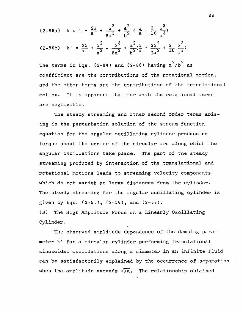
2 2The terms in Eqs. (2-84) and (2-86) having a /b as coefficient are the contributions of the rotational motion, and the other terms are the contributions of the translational motion. It is apparent that for a<<b the rotational terms are negligible.

The steady streaming and other second order terms aris­ing in the perturbation solution of the stream function equation for the angular oscillating cylinder produce no torque about the center of the circular arc along which the angular oscillations take place. The part of the steady streaming produced by interaction of the translational and rotational motions leads to streaming velocity components which do not vanish at large distances from the cylinder.The steady streaming for the angular oscillating cylinder is given by Eqs. (2-51), (2-56), and (2-58).(B) The High Amplitude Force on a Linearly OscillatingCylinder.

The observed amplitude dependence of the damping para­meter k* for a circular cylinder performing translationalsinusoidal oscillations along a diameter in an infinite fluidcan. be satisfactorily explained by the occurrence of separation when the amplitude exceeds /Ta. The relationship obtained

100

from the potential flow model for the change, Ak', in damp­ing parameter with amplitude is

2 - — 2.(4-1) Ak' = ( -i|) (0.16) -4— sinwt { “, V aTTa 23 IT w

1— Jw

+ i c2 2 2 Jto U) u>3+4— -+— | 3-4— +-§■to 2 to I0) w

0) 0)cos2iot (1— — ) (1+ )j S r w a) n i+ ----5---- L--------- ? ------------ ?J >to (1) (*) 0)

3-4— +— | 3+4— +-|b) 2 to 20) to/Xawhere A is the amplitude of oscillation, cosait = 1 - - t t ,2 tot s A

and u) /w= [1--------- . The potential flow model and viscousS TTflow model give about the same results for Ak'.

The separation models do not satisfactorily explain the observed change, Ak, in period parameter with amplitude of oscillation. Both the potential flow model and viscous flow model predict a decrease in Ak with increasing amplitude, but the predicted decrease is much smaller than that observed experimentally. The potential flow model predicts that Akis dependent only upon A//Xa, and the experimental results

15 .of Kimball exhibit that same quality. The viscous flow1/2model gives values of Ak depending on a/(v/w) as well as

A//Xa.

101

The damping parameter results obtained from the separa­tion models indicate that separation is the important factor causing the amplitude dependent damping. The period para­meter results, however, indicate that an important feature of the fluid flow has been overlooked in the formation of the models. It is possible that vortex formation in the separation region is important in causing the decrease in Ak even at amplitudes just above /Xa.

The fact that the viscous flow model gives worse resultsthan the potential flow model is a possible indication thatthe perturbation solution used in the non-separated regionis invalid. It cannot be concluded, however, that viscosityalone will account for the discrepancy between experimentaland theoretical values of Ak. The experimental boundaryeffect noted in Chapter I may give insight into the natureof the decrease in Ak with amplitude. It seems from thediscussion of the boundary effect that steady streaming is .connected with the period parameter results. At highamplitudes the thickness of the steady streaming boundary

2 6layer has been observed to be amplitude dependent. A quantitative explanation of the amplitude dependence of <5 is lacking.

It should be noted also that the experimental method used by Kimball employed two cylinders. It is possible that the size of the decrease in Ak is determined by the inter­action of the two cylinders. It would be instructive to

102

test the effect of changing the distance between the cylinders on Ak.

An important result which has not been mentioned concerns the method employed in the Appendix for the calculation of Ak and Ak' from a knowledge of the force on the oscillating cylinder. The changes in period and logarithmic decrement in oscillatory fluid flow about any object can be calculated from a knowledge of the force on the object by the same _ method used in the Appendix, as long as the mass of fluid displaced by the object is small compared to the mass of the object. Hence, the changes in period and logarithmic decre­ment (or Ak and Ak') are the important quantities to be measured in testing the validity of a theoretically deter­mined force.

In conclusion, the amplitude dependence of Ak' has been explained by a simple model based on the occurrence of separation. The amplitude dependence of Ak is not satis­factorily explained by the same model.

REFERENCES

■*" G. G. Stokes, Trans. Cambridge Phil. Soc. 9_, part 2, 8(1850); Mathematical and Physical Papers (Cambridge: University Press, 188 0 - 1905), iii, p. 1 (hereafter re­ferred to as Papers).

2 J. T. Stuart, J. Fluid Mech. 24, 673 (1966).

C. Y. Wang, Quart. Appl. Math. 23_, 305 £1966).li G. G. Stokes, Paper's, iii, p. 47.

J. T. Stuart, J. Fluid Mech. J24 , 679 (1966).C G. H. Keulegan and L. H. Carpenter, J. Research Natl.

Bur. Standards 6£, 4 23 (1958).7 G. G. Stokes, Papers, iii, p. 38.Q J. T. Stuart, "Unsteady Boundary Layers," Ch. VII

of Laminar Boundary Layers, Ed. L. Rosenhead, (Oxford: Clarendon Press, 1963) (hereafter referred to as "Unsteady Boundary Layers").

9 L. D. Landau and E. M. Lifshitz, Fluid Mechanics (Addison-Wesley: Reading, Mass., 1959), p. 91.

J. T. Stuart, "Unsteady Boundary Layers," p. 392.

11 Yee-Tak Yu, J. of Appl. Phys. 13, 66 (1942).12 T. E. Stelson and F. T. Mavis, Proc. Am. Soc. Civ.

Engr., Engr. Mech. Div., 81, No. 670 (April, 1955).

103

104

^3 J. T. Stuart and L. Woodgate, Phil. Mag. 4_6, 4 0 (1955) .

14 R. G. Hussey, B. J. Good, and J. M. Reynolds, Phys. Fluids 10, 89 (1967).

15 G. R. Kimball, M. S. Thesis, Louisiana State University (1965) (Unpublished).

16 D. P. Thibodeaux, Ph. D. Dissertation, Louisiana State University (1967) (Unpublished).

17 J. M. Andres and U. Ingard, J. Acoust. Soc. Am. 25, 928 (1953).

18 J. M. Andres and U. Ingard, J. Acoust. Soc. Am. 25932 (1953).

19 J. T. Stuart, "Hydrodynamic Stability," Ch. IX of Laminar Boundary Layers, Ed. L. Rosenhead, (Oxford: Clarendon Press, 1963), p. 578.

20 H. Schlichting, Phys. Z. 33_, 327 (1932).21 J. T. Stuart, "Unsteady Boundary Layers," p. 349.

22 E. N. Andrade, Proc. Roy. Soc. London, A 134, 447 (1931).

23 H. Schlichting, Phys. Z. 33_, 327 (1932).Oil Z. Carriere, J. Phys. et. radium, Ser. 6 , 1_0, 198

(1929); Ser. 8 , 1, 68 (1940).2 5 J. Holtsmark, I. Johnsen, T. Sikkeland, and S.

Skavlem, J. Acoust. Soc. Am. 26, 26 (1954).

105

2 6 W. P. Raney, J. C. Corelli, and P. J. Westervelt,J. Acoust. Soc. Am. 2_6, 1006 (195*+).

27 J. Holtsmark, I. Johnson, T. Sikkeland, and S.Skavlem, J. Acoust. Soc. Am. 2T_t 179 (1955).

28 P. J. Westervelt, J. Acoust. Soc. Am. ^5, 951 (1953).29 S. Skavlem and S. Tjotta, J. Acoust. Soc. Am. 27,

26 (1955).

38 P. J. Westervelt, J. Acoust. Soc. Am. ^3, 1672 (1961).

31 L. A. Segel, J. Math. Phys. 39, 189 (1960).

32 J. T. Stuart, "Unsteady Boundary Layers," p. 3 93.3 3 H. Schlichting, Boundary Layer Theory (McGraw-Hill

Book Company, Inc., New York, 1962), 2nd. ed., p. 27 (hereafter referred to as Boundary Layer Theory).

34 M. J. Lighthill, "Introduction. Boundary Layer Theory", Ch. II of Laminar Boundary Layers, Ed. L.Rosenhead (Oxford: Clarendon Press, 1963), p. 63.

3 5 H. Schlichting, Boundary Layer Theory, p. 107.

36 Ibid., p. 109.9 7 Ibid., p. 113.

38 Ibid., p. 29.

39 J. T. Stuart, "Unsteady Boundary Layers," p. 368.4 0 H. Schlichting, Boundary Layer Theory, p. 214.

106

41 Ibid., p. 219. u 2 M. Abramowitz and I. A. Stegun, Eds., Handbook of

Mathematical Functions, Natl. Bur. Stds. Appl. Math. Ser.5 5 (United States Government Printing Office, Washington, D. C. , 196i+), p. 358.

43 Ibid., p. 361.

44 Ibid., p. 361.

45 Ibid., p. 364.4 6 •L. D. Landau and E. M. Lifschitz, oj). cit. , p. 318

APPENDIX

CALCULATION OF Ak AND Ak' FROM THE FORCE EXERTED ON THE CYLINDER BY THE FLUID DURING SEPARATION

The changes in k and k' with amplitude of oscillation can be determined if the force exerted on the cylinder by the fluid during separation is known. In the separation models presented in Chapter III, it was assumed that separa­tion did not occur until the cylinder had moved a distance

1/ 2(Aa) from a position of rest. From t=Q to the separationtime t the force has the form sCA-1) F = - M'k y - M'wk'y ,oJc oJcwhere M' is the mass of fluid displaced by the cylinder, y is the cylinder acceleration, yQ is the cylinder velocity, and kQ and k^ are the low amplitude period and damping para­meters given by Eqs. (1-4). Equation (A-l) is valid only for small damping. The equation of motion of the cylinder is then given by(A-2) My + 4ir2ay = - M'k y - M'wk’yJ c Jc oJ c oJ c

2where 4ir ayc is the linear restoring force, and M is the mass of the cylinder per unit length. In the first approxi­mation the terms on the right hand side of (A-2) may be neg­lected and the function yc (t) is approximately (A*-3) y_(t) - - A coswt,

22 awhere A is the amplitude and w = — — . The second approxima­tion may be found by substituting Eq. (A-3) into the terms on the right hand side of Eq. (A-2).

A-l

A-2

(A-4) yc+ w2yc= - j£- ko<D2Acos<Dt - w 2k^Asinwt,which has the solution

(A-5) yc (t) = - A[1 - T^k^wtlcosuit

Ml M '- ■jyf*<:0w't A sinoit - sinwtM twhere the last term, - k^ Asinuit, is added so that the

cylinder will be at rest at t=Q. We define yQ (t) as follows(A-6) Y o ^ ) = “ ACl - ^gk^wtDcoscot - ^ kQwtAsinwt

M *- 7ft kQAsxnwt When separation occurs the force changes, and the

equation of motion of the cylinder has the form (see Eqs. (3-25) and(3-45))/ * -s . 2 M' 2. A ^ M ' A 2. . . .(A-7) yc+ id yc= - <d koAcosuit - ^ <d r s m u t+K, cosuitsinw t f + K0sintot sincu t 1 + K_sinw t ’ + K., cos2iotsin(D t f l s 2 s 3 s 4 s+ K (-sin2(ot sintu t',

S 2<Dtwhere <d = w/(l - ----— ), t* - t-t , and the K 1 s. ares tt s ’ •constants proportional to M'/M (for the potential flow modelk'= K,-= 0 and k = 1). Using simple trigonometric identities O w oone can change Eq. (A-7) to the form

(A-8 ) yc+ <o2yc= - ~ (D2kQAcos(Dt - 2k^sincot

— - K1+ tt— Csin(wt+(D t ’) - sin(iDt-io t 1)] i s sK2+ -k— [cos((Dt-w t 1) - cos(wt+w t')] + K 0sinai t f 2, s s 3 s

A-3

(A-8) cont'd K4+^— Csin(2tdt+o) t 1) - sin (2tot-w t')] 1 s sK5+ 75— Eeos ( 2u>t-o) t) - eos(2o)t+o) t 1)]I s s

The function y (t) during separation may then be written in cthe form(A-9) y = y (t) + C, coswt + C 0sino)t + T-, sin(o)t+<D t ' ) c o 1 2 l s

+ T 0sin(ait-u) t f) + T0cos(a)t~a) t')2 s 3 s+Tucos(cot+o) t T) + TcSinw t 1*4 S 0 S

+ T c sin( 2o>t+a> t') + T sin(2wt-w t ’)6 s 7 s+ T g C o s ( 2 u ) t - a ) s t r ) + T g C o s ( 2 t u t + o)s t f ) ,

where(A-10a) T,= - tA

2 (2o)0) +o)2)s sK1 1(A-lOb) T9= - ^ ----- ±-T-

(2u)(o -u> ) s s

K 2(A-lOc) T„ = tt—3 2 (2b)0) - w 2 )S S

(A-lOd) Tu= J - ---- ^(2o)(o +o) ) s s

K3(A-lOe) T c=5 2 20) - 0) sK4 1(A-lOf) T 6= ----- -~7~ --- — 7

3o> +4o)o) +u> s s

(A-lOh) Tg = - / . 1 -y3d) -Haiti) +a>S S

CA-lOi) Tg= Y- - g -1- ■; 2OO) + 4(i>0) +(1)S S

and and C are constants determined by the conditions thatposition and velocity of the cylinder must be continuous

at t=t (t'=Q). These conditions lead to the following sequations(A-lla) (C,+ T_+ Tj, ) (-co suit ) + (C„+T- + T „ )(-sinoit )1 3 H s 2 1 2 s

= (Tg+ ) sin2o)ts+ (Tg + Tg)cos2wts

(A-llb) (C..+ T„+ T. ) (sinoit ) + (G„+ Tn + T, ) (-cosut )1 3 4 s 2 1 2 stl) (D 0)

= — (T, - T„)cosoit + — (T«- Tu )sintnt + — T, a) 1 2 s 0) 3 4 s t i ) 5u o)

+ C(2+— )TC+ (2-- —)T„3cos2uita) 6 to / s

ID. tD_-[ (2-----)T0 + (2+— )TQ]sin2d)ttu 8 a) 9 s

Equations (A-ll) are readily solved to give111 9

(A-12a) C-,= -(T- + Tu ) + — (To- Tu )sin wt-+ -2. T sinoit1 3 4 a) 3 4 s t i i s S0)

+ — (T, - T 0)sinoit cosuit - (Tc+ T7)sino)t o i l 2 s s o / s0) 0)

+ [(1 + — )TC+ ( 1 --- —)T„]sinoit cos2o)t0) 6 0) 7 S S

u o)- (Tq+ T q )cosut -C (1----)Tq+ (1+ — )TQ]sinu)t sin2u)t8 9 s ti) 8 0 ) 9 s !

A - 5

“s 2(A-12b) C„= - (T,+ T,) - -2. (T,- T9 )cos ut2 1 I <o X 2 sto "to

- — (T~- T„)sintot costot T ccostotto 3 4 s s to o sto to

- (Tc+ T7 )costot - [(1+— )TC + (1- — >T7 ]costot cos2totb / s to b to / s s“e+ (T0+Ta) sintot +[ (1— — >Tq+(-1+— 24~TQ"]<30Su>t sin 2 tot 8 9 s co 8 to 9 s s

The position of the cylinder is determined by Eq. (A-9)between t=t and t= t , the latter time correspondings co sto u t'= n. At in t' = ir the separation angle returns to5 Szero, and the equation of motion of the cylinder once again becomes

• • 2 M 1 2 ' M i 2(A—*+ > y + to y = - k to Acostot - tt— m k'Asintot.-'C C M O M OFor the remainder of the half cycle the position of the cyl­inder is given by

. < i

(A-13) y = y (t) +A-,cosiot + A7sintot.JC ■'o 1 2 7

where A- and A2 are determined by the conditions that ycand yc be continuous at t = ^ - t g . Application of those condi­tions leads to

“s 2 (A-14a) A,= C,- T_- T„+ -=■ (T0- Tu )sin totJL ± d 4 (0 • d M- sto <0

- — (T-,- T 7)costot + — Tj-sintot to 1 2 s to 5 sto to

- (Tc+ T7 ) sintot +[ (1+ — )Tr + (1 - ~ ) T 7]sintot cos2totb / s to b to / s sto to

+ (T0 +T„) costot +C(1- — ^)Tq + (1+— )TQ]sintot sin2<ot y y s to "o to y s sto _ to ^

(A-14b) A7= C7-T, - T 0+ — T Rcos(ot - — (-T*-T-7)cos <ot_2 2 1 2 t o 5 s t o l 2 s(A —14-b) cont'd

A-6

OJ+ — (T0- T,.)sinut cosut + (Tc+T7 )coswte co a H s s b / s

w n.+ (T0+Tq)sincot + [(1 + — ) T c+ ( 1 ---2.)T7] cosut cos2utb y S. U) D 0) / S 5

0) dig+ [(1 - — )Tq+ (1 + — )Ta]sin2ut cosut to 8 co 9 s s

Substitution of the expressions (A-12) for and C2 into Eqs. CA-14) yields

2tiis 2(A-15a) A,= - 2(T„+ Tu ) + — - (T«- Tu )sin ut 1 o 4 co o 4 s

■2“s+ T csintot - 2(TC+ T«)sincotto 5 s 6 7 s(0 (0

+ 2 sincot cos2ut [(1+— )TR+ < 1 ----)T7]s s u b u /“s 2(A-15b) A2= -2(T1+ T 2 ) (Tx- T 2 )coszuts

+ 2 (Tg+ Tg )sinutsHI U

+ 2 C( 1 -)Ta + (1 + — )TQ]sin2ut cosutu o u y____ _ s sFrom Eqs. (A-13) and CA-6 ) the cylinder position and

velocity at the end of a half cycle are given byM'k' M'Ak

(A-16a) yc (y) = - A t l uj I c o s u J ^-^^Isinuy

M T T • T- k'AsinuTr + A-,cosu-k- + A0sinu-*-2H o 2 1 2 2 2

M'k'(A— 16b) yc (-2») "0“(oA[l —■ ■oiyp]sinta

A M ' , T T" 2tT" o“7 a,COSO)Y

A-7

M • T • T T- - ^ k oa)Asinuj-?j- - toA^sintoy +u)A2COSa>-?p,

where t is the period of oscillation. We let t = t q + A t ,

where t q = 2n/u would be the period i f no fluid were present.Assuming M'<<M, we let sinu)-^ =01 * and cosw^ - 2 1, and obtain,to first order in M'/M,f A -> n \ . At M ' , ^2(A-17 ) tanio- — = kQir -

so thatMl tj 2^2(A-18) A t = rr— k ------- T--.......M 00) id A

The period is then given byMT(A-19) t =x + J - k - J ,o M 0(u (uA

2itwhere t q = — . Using the expression( t 2 - t ^ )

(l-3a) k = ° M , °2

and the equation id = —g— one can then easily find2M ^2(A-20) k = k - ig-, -4 o irM' A

The last term in equation (A-20) is the change in k with amplitude(A-21) Ak = - | g f

The position at the end of a half cycle is, from Eq.(A-16a),

M'k'(A-22) yc <£)«A[l -

Then at the end of a complete cycle the amplitude will beM'k'cM ,,J ‘“1'A[1 - —r, — itII — 2An . The logarithmic decrement is thus

A-8

CA-23) D = ln{ - A H rk .,, j;— )AC 1 - H -------- J T ]

so thatm t 2A,. , . 1(A-24) D - k » + _x _

The damping parameter, k' , is related to D by the expression

(l-3b) k- = D = ^ D ,

so that(A-25) k' = k£ + ^ .The change, Ak', in k 1 with amplitude is then

2M ^1(A-26 ) Ak' = —ttt- tAttM1 AExpressions for A^ and Ag are given in Eqs. (A-10).

Those equations can be combined with (A-21) and (A-26) togive the following expressions:

u m “ sinwtCA-27a > ik' = ^ { jS. K 3 -5 Sy

0 ) - OJsO O(1 - — sin wt ) (1 + — sin wt )lv r s j. to s i

" 2K 2 L 9 2 2 J 2o)cu - to 2wa) + cuS S S s

+ \ K^siiKot C - 2 - i ----— J- - j-i----— 2- 33a) +4-o)C0 +o> 3to -HcDti) +cos s s s

(D 0) ■(1 - (i + -£)

+ -s- Kusinu)t cos2u>t [— =------- 9 - — *---------*- 1 >3to +0) 3w +4ojo) +0)s s s s

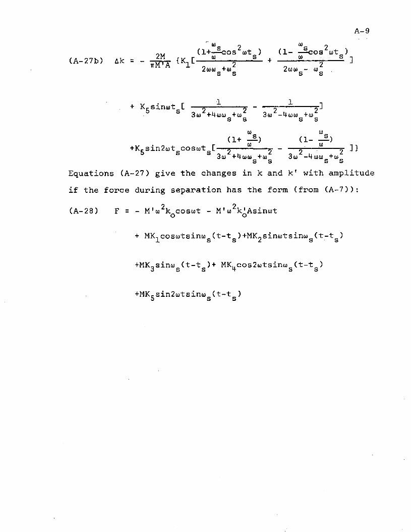
+ K,-sinu)t [ — s— s- - — s— j]3o) +4(ou) +(») 3u> -4o)(o +ws s s s

0) 0)(1+ ^2.) (1- ^2.)

+KcSin2tot costot [— *-------- *--- — rf— — -- tt ]}3o) +4(1)0) +o) 3oi -4o)0) +o) s s s s

Equations (A-27) give the changes in k and k ’ with amplitude if the force during separation has the form (from (A-7)):

(A-28) F = - M'oi^k coso)t - M ’ to^k' Asinwto o

+ MK, costotsinto (t-t ) +MK0sino)tsinu) (t - t )1 s s 2 s s

+MK0sinto (t-t )+ HKkcos2o)tsino) (t-t ) 3 s s 4 s s

+MKcsin2(otsino) (t-t ) j s s

VITA

John Stephen Bosnak was born in Alton, Illinois, on February 14, 1941. He attended elementary and high schools in Alton and was graduated from Alton Senior High School in 1959. He entered the University of Missouri School of Mines and Metallurgy, Rolla, Missouri, in September, 1959, and received a Bachelor of Science degree in physics in 1963. He entered the Graduate School of Louisiana State University in September, 1963, held an N.D.E.A. fellowship in the Department of Physics and Astronomy during his first three years of graduate study, and served as Instructor from September, 1966, until June, 1967. He is presently a can­didate for the degree of Doctor of Philosophy in the Depart­ment of Physics and Astronomy.

107

EXAMINATION AND THESIS REPORT

Candidate: John Stephen Bosnak

Major Field: Phy s i c s

Title of Thesis: "A Theoretical Study of the Force Exerted by a Viscous Fluid on an Oscillating Cylinder"

Approved:

Major Professor and Chairman

Dean of the Graduate School

EXAMINING COMMITTEE:

Date of Examination:

July 20, 1967