Embed Size (px)
DESCRIPTION
In this report, the effect of temperature dependent variable viscosity on Magnetohydrodynamic (MHD) natural convection flow of viscous incompressible fluid along a uniformly heated vertical wavy surface has been investigated. The governing boundary layer equations with associated boundary conditions for phenomenon are converted to non-dimensional form using a suitable transformation.
Citation preview

NUMERICAL INVESTIGATION ON NATURAL CONVECTIONN FROM AN OPEN RECTANGULAR CAVITY CONTAINING A HEATED CIRCULAR CYLINDER
ABSTRACTIn this report, the effect of temperature dependent variable viscosity on
Magnetohydrodynamic (MHD) natural convection flow of viscous incompressible fluid along
a uniformly heated vertical wavy surface has been investigated. The governing boundary
layer equations with associated boundary conditions for phenomenon are converted to non-
dimensional form using a suitable transformation. The resulting nonlinear system of partial
differential equations are mapped into the domain of flat vertical plate and then solved
numerically employing the implicit finite difference method, known as Keller-box scheme.
The numerical results in terms of the skin friction coefficient, the rate of heat transfer, the
velocity and temperature profiles as well as on the streamlines and the isotherms over the
whole boundary layer are shown graphically for the effects of the pertinent parameters, such
as the viscosity parameter (ε), the magnetic parameter (M), the amplitude of the waviness (α)
of the surface and Prandtl number (Pr). Numerical results of the local skin friction coefficient
and the rate of heat transfer for different values are presented in tabular form. The
programming language LAHEY FORTRAN 90 will be used and an in finite difference
programming code will be modified to fit the present problem. The post processing software
TECHPLOT has been used to display the numerical results graphically. Comparisons with
previously reported investigations are performed and the results show excellent agreement
Nomenclature
Cfx local skin friction coefficient
Cp specific heat at constant pressure
f dimensionless stream function
g acceleration due to gravity
Gr Grashof number
k thermal conductivity
L characteristic length associated with the wavy surface
M magnetic parameter
Nux local Nusselt number

P pressure of the fluid
Pr Prandtl number
T temperature of the fluid in the boundary layer
Tw temperature at the surface
T temperature of the ambient fluid
u,v
velocity component in x
,y
direction
u , v dimensionless velocity component in x, y direction
x,y
Cartesian co-ordinates
x , y dimensionless Cartesian co-ordinates
Greek symbolsa amplitude of the surface waves
b volumetric coefficient of thermal expansion
b0 applied magnetic field strength
e viscosity variation parameter
h dimensionless similarity variable
q dimensionless temperature function
m dynamic coefficient of viscosity
m dynamic viscosity of the ambient fluid
n kinematic coefficient of viscosity
r density of the fluid
tw shearing stress
y stream function
(x) surface profile function defined in equation (2.1)
Subscripts
w wall conditions
ambient conditions
Superscripts
Prime (¿
) differentiation with respect to η.

CHAPTER-1
INTRODUCTION
1.1 GENERALHeat is one kind of energy which is very much useful to everyday life. Energy can exist in
numerous forms such as heat, mechanical, kinetic potential, electrical, magnetic, chemical
and nuclear, and their sum constitutes the total energy E of a system. Heat transfer is that
thermal science which seeks to predict the energy transfer which may take place between
material bodies as a result of a temperature difference. Thermal science includes
thermodynamics and heat transfer. Thermodynamics consider only system in thermal
equilibrium. Two systems are said to be in thermal equilibrium with one another if no heat
transfer occurs between them in a finite period when they are connected through diathermal
(non-adiabatic) wall. Heat transfer will take place from the body with higher temperature to
that with the lower temperature, if they are permitted to interact through a diathermal wall.
Heat transfer is commonly associated with fluid dynamics and it also supplements the laws of
thermodynamics by providing additional experimental rules to establish energy transfer rates.
The concept of temperature distribution is essential in heat transfer studies because of the
fact that the heat flow take place only wherever there is a temperature gradient in a system.
The heat flux is defined as the amount of heat transfer per unit area per unit time, which can
be calculated, from the physical laws relating the temperature gradient and the heat flux.
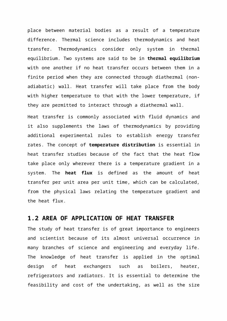
1.2 AREA OF APPLICATION OF HEAT TRANSFERThe study of heat transfer is of great importance to engineers and scientist because of its
almost universal occurrence in many branches of science and engineering and everyday life.
The knowledge of heat transfer is applied in the optimal design of heat exchangers such as
boilers, heater, refrigerators and radiators. It is essential to determine the feasibility and cost
of the undertaking, as well as the size of equipment required to transfer a specified amount of
heat in a given time. The electric and electronic plants require efficient dissipation of thermal
losses. Through heat transfer analysis is most important for the proper sizing of fuel elements
in the nuclear reactor cores to prevent burnout. The successful fly of aircrafts also depends
upon the case with which the structure and engines can be cooled. The designs of chemical
plants are taken on the basis of heat transfer. Accurate heat transfer analysis is required in the
refrigeration and air-conditioning applications to calculate the heat loads and to determine the
thickness of insulation to avoid excessive heat gains or losses. It is also requires a through
knowledge of heat transfer for the proper design of the solar collectors and associated
equipments to utilize the so abundantly available solar energy. Civil engineers should also
take care of the thermal effects in buildings and structures. The Human body is constantly
rejecting heat to its surroundings and human constant is closely depends on the rate of this
heat rejection. Many ordinary house hold machinery are designed in whole or part by using
the principle of heat transfer. This is why heat transfer is of great importance in the field of
science and engineering.
1.3 MECHANISM OF HEAT TRANSFERThe heat transfer takes places by three distinct mechanisms or modes: Conduction,
convection and radiation. Conduction is the transfer of energy from the more energetic
particles of a substance to adjacent less energetic ones as a result of interactions between the
particles. Heat conduction of heat transfer takes place by two mechanisms (i) By molecular
interaction whereby the energy exchange takes place by the kinetic motion or direct impact of
molecules. Molecules at a relatively higher temperature level losses energy to adjacent
molecules at lower temperature levels. This type of heat transfer always exists so long as
there is a temperature gradient in a system comprising molecules of a solid, liquid or gas.
(ii) By the force of ‘free’ electrons as in the case of metallic solids. The metallic alloys have a
different concentration of free electrons and their abilities to conduct heat are directly
proportional to the concentration of free electrons in them. The free electron concentration on
non-metals is very low. So, the pure metals are good conductors such as copper, silver etc.
Pure conduction is found only in solids. Since heat conduction is proportional to temperature
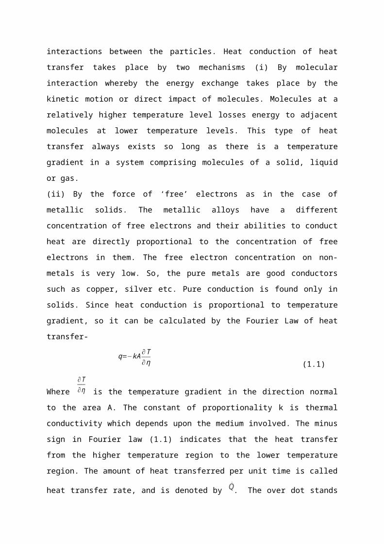
gradient, so it can be calculated by the Fourier Law of heat transfer-
q=−kA ∂T∂η (1.1)
Where
∂T∂η is the temperature gradient in the direction normal to the area A. The constant of
proportionality k is thermal conductivity which depends upon the medium involved. The
minus sign in Fourier law (1.1) indicates that the heat transfer from the higher temperature
region to the lower temperature region. The amount of heat transferred per unit time is called

heat transfer rate, and is denoted by . The over dot stands for time derivative. When the
rate of heat transfer is known then the total amount of heat transfer Q during a time step t
can be determined using the equation
(1.2)
where is constant. The above equation (1.2) become
(1.3)
In fact, the combined effects of these three mechanisms of heat transfer control temperature
distribution in a medium. A brief description of heat convection is given follows.
1.4. THERMAL CONDUCTIVITYThe thermal property specific heat Cp as a measure of a material’s ability to store thermal
energy. Similarly, the thermal conductivity k is a measure of a material’s ability to conduct
heat. That is, the thermal conductivity of a material can be defined as the rate of heat transfer
through unit thickness of the material per unit area per unit temperature difference. For
example, k = 0.607 N/m2 C for water and k = 80.2 W/m2 C for iron at room temperature,
which means that iron can conducts heat more than 100 times than water can. That is water is
a poor heat conductor relative to iron. Materials like copper, silver are good heat conductor as
well as good electric conductor and have high values of thermal conductivity. Materials like
Rubber, wood are poor heat conductors and have low values of conductivity. The rate of heat
conduction through a medium depends on the geometry of the medium, it’s thickness and the
material and as well as the temperature difference across the medium.
1.5 CONVECTION HEAT TRANSFERConvection is the mechanism of heat transfer through a fluid in the presence of bulk fluid
motion resulting from the temperature difference. This type of heat transfer is called
convection. The convective heat transfer is divided into two branches: the natural convection
and the forced convection. If the fluid flow in convection occurs naturally, the convection is
called natural (or free) convection. In this case fluid motion is set up by buoyancy effects
resulting from the density variation caused by the temperature difference in the fluid and
gravitational force. On the other hand if the fluid motion is artificially created by means of
external source like a blower or fan, the heat transfer mode is called forced convection. In
case of forced convection, the fluid is forced to flow over surface or in a pipe by external
means such as a pump or a fan.
Heat transfer through a fluid is by convection in the presence of bulk fluid motion and by
conduction in the absence of fluid motion. So, conduction in a fluid can be viewed as the
limiting case of convection resulting to the case of quiescent fluid. Since at the solid surface
there is no fluid motion.
So the heat transfers between the solid surface and the fluid at the surface can take place only
by conduction, the heat transfer by convection is always accompanied by conduction.
The temperature distribution in the natural convection depends on the intensity of the fluid
currents that is dependent on the temperature potential itself. So the qualitative and
quantitative analysis of natural convection heat transfer is very difficult. Numerical
investigation rather than theoretical analysis is more effective in this field. In the nature, two
types of natural convection can be observed. One is external free convection that is caused by
the heat transfer interaction between a single wall and a very large fluid reservoir adjacent to
the wall. Another is the internal free convection, which befalls within an enclosure.
The thermo-fluid fields developed inside a cavity depend on the orientation and physical
figure of the cavity. Re-viewing the nature, practical application and the phenomena of
enclosure can be organized into two classes. One of these is the enclosure heated from the
side such as solar collectors, double wall insulations, laptop cooling system and air
circulation inside the room. Another one is the enclosure heated from below which happens
in geophysical system like natural circulation in the atmosphere, the hydrosphere and the
molten core of the earth.
Since in this case convection is the study of heat transport processes affected by the flow of
fluid, it is clearly a field at the interface between two older fields: heat transfer and fluid
mechanics. At first it is required to reexamine the historic relationship between fluid
mechanics and heat transfer at the interface to reviewing the foundations of convective heat
transfer methodology. Heat transfer and fluid mechanics have been enjoying a symbiotic
relationship in their parallel development during the past 100 years.
In convection mode of heat transfer energy exchange occurs between the particles by
convection current. That is, when fluid flows over a solid body or inside a channel while
temperatures of the fluid and the solid surface are different, heat transfer between the fluid
and the solid surface takes place as a consequence of the motion of the fluid relative to the
surfaces. Considerable effort has been done for the diversity of the studies related to
convection mode heat transfer, in which the relative motion of the fluid provides an
additional mechanism for the transfer of heat and materials. Convection is obviously coupled
with the conductive mechanism, since though the fluid motion modifies the transport process,
the eventual transfer of heat from one fluid element to another in it’s neighborhood is through
conduction.
The fluid flow may occur for instance, a fan, a blower, the wind or the motion of the heated
object itself. Such problems are encountered very frequently in technology where heat
transfer to or from a body is often due to an imposed flow of a fluid at a temperature different
from that body. It has wide range of applications in compact heat exchanger, central air
conditioning system, cooling tower, gas turbine blade, internal cooling passage, chemical
engineering process industries, nuclear reactors and so many cases. If, no such externally
induced flow is provided and the flow arises “naturally” simply due to the effect of a density
difference, resulting from a temperature difference, in a body force field, such as gravitational
field, the process is termed as natural or free convection. The density difference gives rise to
buoyancy effect due to which the flow is generated. A heated body, which is cooling in
ambient air, generates such a flow in the neighboring region surrounding it. Again, the
buoyant flow arising from heat rejection to the atmosphere and to other ambient media. Free
convection heat transfer occurs in many engineering applications, such as heat transfer from
hot radiators, refrigerator coils, transmission lines, electric transformers, electric heating
elements, electronic equipment and so many cases.
The buoyancy force, which rises as the results of the temperature difference and which cause
the fluid flow in free convection, also exists when there is a forced flow. The convection heat
transfer cannot be dominated by pure force nor pure free convection, but by a combination of
two, which is referred as combined or mixed convection. However, in some cases, these
buoyancy forces do have a significant influence on the flow and consequently on the heat
transfer rate. In that case the flow about the body is a combination of forced and free
convection, such flows are referred to as mixed convection. In many cases, heat transfer from
one fluid to another fluid through the walls of pipe occurs in many practical devices. In this
case, heat is transferred by convection from the hotter fluid to the one surface of the pipe.
Then heat is transferred by conduction through the walls of the pipe. That is, finally, heat is
transferred by convection from the other surface to the colder fluid.

1.5.1 SPECIFIC HEAT
The specific heat of a substance is defined as the amount of heat required to raise the
temperature of a unit mass of the substance by one degree and denoted by C. So, C=∂Q
∂T,
where ∂Q is the amount of heat added to raise the temperature by ∂T . There are two
important specific heats in thermodynamics:
Specific heat at constant volume: Cv=(∂Q
∂T )v and specific heat at constant pressure:
C p=(∂Q∂T )
p. The ratio of specific heat is denoted by n and
ν=C p
C v .
1.5.2 VISCOSITY
The normal force per unit area is said to be the normal stress or pressure and the tangential
force per unit area is said to the shearing stress. A fluid is said to be viscous if it holds normal
stress as well as shearing stress. Again, a fluid is said to be in viscid if it does not exert any
shearing stress whether at rest or in motion. Due to shearing stress a viscous fluid produces
resistance to the body moving through it as well as between the particles of the fluid itself.
Water and air are treated in viscid fluids where as blood and heavy oil is treated as viscous
fluids.
The simplest flow situation involving a non-zero viscosity is laminar flow along flat wall. In
this case, fluid layers slide parallel to area another molecular layer adjacent to the will being
stationary. The next layer out from the wall slides along this stationary layer and its motion is
impeded or slowed because of the frictional shear between these layers. Continuing outward,
a distance exists where the retardation of the fluid due to the presence of the wall is no longer
exist. The difference in velocity between two adjacent fluid layers produces a shear stresst.
Newton postulated that this stress is directly proportional to the velocity gradient normal to
the plane as follows
τ=μfdudy
Where μ f is the coefficient of dynamic viscosity or simply dynamic viscosity?
Kinematical viscosityn:
The ratio of dynamic viscosity to density is called the kinematical viscosity n and
ν=μm
ρ
where μm is the mass based viscosity coefficient.
1.5.3 THERMAL DIFFUSIVITY
A useful function of thermal conduction k contains a quantity a, called the thermal
diffusivity. Thermal diffusivity expresses how fast heat scatters through a material and is
defined as
α= kρC p
Here a is the ratio of the thermal conductivity to the thermal capacity (heat stored per unit
volume) of the material. Thermal capacity will have a large thermal diffusivity. That is
thermal energy diffuses rapidly through matter with high a and slowly through those with
low a.
1.5.4 INTERNAL AND EXTERNAL FLOWS
Fluid flow is classified into two types (i) Internal and (2) External, depending a whether the
fluid is forced to flow in a confined channel or over a surface. The internal flow is in a
channel bounded by solid surfaces except, possibly, for an inlet and exit. Fluid flow through a
pipe, in an air conditioning duct is internal flow. Viscosity in fluid flow dominates the
internal flow. The internal flow configuration represents a convenient geometry for the
heating and cooling of fluids used in the chemical processing, environmental control and
energy conversion areas. An unbounded fluid flow over a surface is external flow. The flows
over curved surfaces such as sphere, cylinder, airfoil or, turbine blade are the example of
external flow. The viscous effects are limited to boundary layers near solid surfaces in
external flows.
1.5.5 BOUNDARY LAYER
Since convection heat transfer occurs due to fluid flow, so there must be a boundary layer in
convection mode of heat transfer. If a fluid flows over a body, the nearest region of the
surface strongly influenced by the convective heat transfer. The boundary layer concept
frequently is introduced to the velocity and temperature fields near the solid surface in order
to simplify the analysis of convective heat transfer. So, there are two different kinds of
boundary layers exist in convective heat transfer: the velocity boundary layer and the thermal
boundary layer.
Velocity Boundary Layer:
The region of the flow above the plate bounded by in which the effects of the viscous
shearing forces caused by fluid viscosity are felt is called the velocity boundary layer. The
boundary layer thickness,, is typically defined as the distance y from the surface at which
the velocity of fluid equal to ninety percent of the free stream velocity v of the fluid.
The hypothetical line v = 0.99U divides the flow over a plate into two regions: The boundary
layer region where the viscous effects and the velocity changes are significant and the
irrotational flow region where the frictional effects are negligible and the velocity remains
essentially constant.
Thermal Boundary Layer:
Like velocity boundary layer, the thermal boundary layer is defined as the region near a
surface in which a temperature gradient exists. Considering the fluid over a flat surface
shown in above Figure. The temperature of the fluid at the leading edge is T.
But the fluid particles in contact with hot wall attain thermal equilibrium with the wall .These
fluid particles impart thermal energy to the adjacent fluid layer and so on far from the wall.
The transfer of heat between successive fluid layers gradually diminishes with increasing
distance from the wall until it become negligible. At this point the fluid temperature must
equal to the free stream temperature T . The thermal boundary layer is defined by fluid
temperatures T that satisfy the relation
1.6 HISTORICAL BACKGROUNDEverybody would think that the nature of heat is one of the first t, being understood by
mankind. Heat has always been perceived to be something that produces in us a sensation of
warmth. But it was only in the middle of the nineteenth century when men had a true physical
understanding of the nature of heat. Kinetic theory was developed at that time, which treats
molecules as tiny balls that are in motion and thus possess kinetic energy. Heat is then
defined as the energy associated with the random motion of atoms and molecules. But it was
suggested in the eighteenth and early nineteenth centuries that heat is the manifestation of

motion at the molecules level, the prevailing view of heat until the middle of the nineteenth
century was based on the caloric theory proposed by the French chemist Antoine Lavoisier
(1743 - 1794) in 1789. The caloric theory asserts that heat is a fluid-like substance (called).
The caloric that is a mass less, colorless and tasteless substance that can be poured from one
body into another. When caloric was added to a body, its temperature increased and if caloric
was removed from a body, its temperature decreased. If a body could not contain any more
caloric or a glass of water could not dissolve any more salt or sugar, the body was said to be
saturated with caloric. This idea of saturated liquid or vapor is still in use today.
But in 1798, the American Benjamin Thomson (1753-1814) showed in his paper that heat can
be generated continuously through frictions. Several others also challenged the validity of the
caloric theory. At last in 1843 Englishman James P. Joule finally convinced all the
contemporary researchers that heat was not a substance after all. Although the caloric theory
was a wrong idea but it contributed greatly to the development of thermodynamics and heat
transfer.
1.7 ENGINEERING HEAT TRANSFERHeat transfer equipment such as heat exchanger, boilers, condensers, radiators, heaters,
furnaces, refrigerators and solar collectors designed primarily on the basis of heat transfer
analysis. The heat transfer problems can be considered in two groups: (1) rating problem and
(2) sizing problems. The rating problems deal with the determination of the rate of heat
transfer for an existing system at a specified temperature difference. The sizing problems deal
with the determination of the size of a system in order to transfer heat at a specified rate for a
specified temperature difference.
An engineering device or process can be studied in two way: (1) Experimentally (testing and
taking measurements) and (2) Analytically (by analysis or (computation). The experimental
approach deal with the actual physical system and desired result in quantity is determined by
measurement, within the limits of experimental error. This approach is expensive, time
consuming and impractical. On the other hand we are analyzing in the analytical process may
not even exist. The analytical approach (including numerical approach) has the advantage
that it is fast and inexpensive, but the results obtained are subject to the accuracy of the
assumptions, approximation and idealizations made in the analysis. In engineering studies,
often a good result is obtained by reducing the choices to just a few by analysis and then
verifying the results experimentally.

CHAPTER 2
2.1 LITERATURE REVIEW
Natural convection in open cavities has become important to the researchers of science and
thermal engineering problems. For example, in the design of electronic devices, solar energy
receivers, uncovered flat plate solar collectors having rows of vertical strips, geothermal
reservoirs, etc. Several experiments and numerical calculation have been presented for
describing the phenomenon of natural convection in cavities for two decades. Those
researches have been focused to investigate effect on flow and heat transfer for different
Rayleigh numbers, aspect ratios and tilt angels. In one case the natural convection in an air
filled, differentially heated inclined square cavity with a diathermal partition placed at the
middle of its cold wall was numerically studied for Rayleigh number 103 to 105. Frederick R.
L. (1989) observed that due to suppression of convection, heat transfer reductions up to 47
percent in comparison to the cavity with partition. Kangni et al (1991) studied laminar natural
convection and conduction in enclosure with multiple vertical partitions theoretically. This
study has done for Rayleigh number Ra in the range 103107, Pr = 0.72 (air), aspect ratio 520,
cavity width 0.10.9 and partition thickness 0.010.1. Those researchers found that the heat
transfer decreases with increasing partition number at high Raleigh number for all
conductivity ratios Kr and heat transfer decreases with increasing partition thickness C at all
Ra except in the conduction regime where the effect is negligibly small. The offender
partitions are less effective in decreasing the heat transfer. In this case the Nusselt number is
also a decreasing function in the aspect ratio.
The effect of a horizontal baffle placed on hot (left) wall of a differentially heated square
cavity determined by Tasnim and Collins (2004).The result has been found that adding baffle
on the hot wall can increase the rate of heat transfer by as much as 31.46 percent compared
with a wall without baffle for Ra = 104. When Ra = 105 the increase in heat transfer is 15.3
percent for the same baffle length and the increases. Heat transfer is 19.73 percent, when the
longest baffle is attached at the middle of the cavity. The steady-state heat transfer by natural
convection in partially open inclined square cavities was studied by Bilgen and Oztop (2005).
Due to the wide variety of applications of natural convection processes, the natural
convection in fluid-filled rectangular enclosures has received considerable attention over the
past several years. These applications span such diverse as solar energy collection, nuclear

reactor operation and safety, the energy efficient design of building, room and machinery
waste disposal, fire prevention and safety. The heat transfer induced by oscillation has been
studied by a number of researchers due to it’s many industrial applications, such as
bioengineering, chemical engineering and so forth. Numerical study on unsteady natural
convection in a partially heated rectangular cavity has done by Kuhn and Oosthuizen (1987).
They found that as the heated location moves from the top to the bottom, the Nusselt number
increases up to a maximum and then decreases. Lakhal et al. (1999) studied the transient
natural convection in a square cavity partially heated from side. At first, the temperature was
varied sinusoidal with time while at the second time; it varies with a pulsating manner. In the
result he found that the mean values of heat transfer and flow intensity are considerably
different with those obtained stationary regime. Le Quere et al. (1981) studied the effect on
the flow field and heat transfer of the Grashof number varied from 104 to 3107; the
temperature difference between the cavity walls and ambient changed from 50 to 500 K, the
aspect ratio varied between 0.5 and 2 and the inclination angle of the cavity was modified
from 0 to 45 (for 0 the wall opposite the aperture was vertical and the angles were taken
clockwise). In the results of the paper it is viewed that the Nusselt number diminished with
the increase in the inclination angle and that the unsteadiness in the flow takes place for
values of the Grashof number greater than 106 and inclination angles of 0. Showole and
Tarasuk (1993) studied experimentally and numerically, the natural steady state convection in
a two dimensional isothermal open cavity. They found the experimental results for air,
varying the Rayleigh number from 104 to 5.5105, cavity aspect ratios of 0.25, 0.5 and 1.0
and inclination angles of 0o, 30, 45o and 60 (for 0, the wall opposite the aperture was
horizontal and the angles were taken clockwise). They calculated the numerical results for
Raleigh numbers between 104 and 5.5105, inclination angles of 0 and 45 and an aspect
ratio equal to one. In the result it is seen that for all Rayleigh numbers, the first inclination of
the cavity caused a significant increase in the average heat transfer rate, but a further increase
in the inclination angle caused very little increase in the heat transfer rate. In another result it
is observed that, for 0, two symmetric counter rotating eddies were formed, while at
inclination angles greater than 0, the symmetric flow and temperature patterns disappear.
Similarly Mohamad (1995) investigated the natural convection in an inclined two-
dimensional open cavity with one heated wall opposite the aperture and two adiabatic walls
numerically. The researcher analyzed the influence on fluid flow and heat transfer, with the
inclination angle in the range 10o – 90o (for 90o the wall opposite the aperture was vertical and

the angles were taken clockwise), the Rayleigh number from 103 to 107m and the aspect ratio
between 0.5 and 2. The investigation concludes that the inclination angle did not have a
significant effect on the average Nusselt number from isothermal wall , but a substantial one
on the local Nusselt number. Polat and Bilgen (2002) investigated the conjugate heat transfer
by conduction and natural convection in an inclined, open shallow cavity with a uniform heat
flux in the wall opposite to the aperture. The studied parameter were: the Rayleigh number
from 106 to 1012, the conductivity ration from 1 to 60, the cavity aspect ratio from 1 to 0.125,
the dimensionless wall thickness from 0.05 to 0.20, and the inclination angle from 0 to 45
from the horizontal (for 0, the wall opposite the aperture was vertical and the angles were
taken counterclockwise).
Le Quere et al. (1981) studied thermally driven laminar natural convection in enclosures with
isothermal sides, one of which facing the opening. In that case the primitive variables and
finite difference expressions are used to treat the problems with large temperature and density
variations. The computational area was an enlarged domain comprising a square open cavity
and a far field surrounding it. Penot (1982) investigated a like problem using stream function
vortices formulation. Like Le Quere et al. (1981) he also used an enlarged computational
domain with approximate boundary conditions. Chan and Tien (1985a) investigated a square
open cavity numerically, which had an isothermal vertical heated side facing the opening and
two adjoining adiabatic horizontal sides. To obtain the satisfactory solutions in the open
cavity the boundary conditions at for field were approximated. Chan and Tien (1985b)
investigated shallow open cavities and made a comparison study using a square cavity is an
enlarged computational domain. In the result they observed that for a square open cavity
having an isothermal vertical side facing the opening and two adjoining adiabatic horizontal
sides. Satisfactory heat transfer results could be obtained, especially at high Rayleigh
numbers.
Mohammad (1995) investigated inclined open square cavities, by considering a restricted
computational domain. The gradients of both velocity components were set to zero at the
opening plane in that case which were different from those of Chan and Tien (1985a). In the
result he found that heat transfer was not sensitive to inclination angle and the flow was
unstable at high Rayleigh numbers and small inclination angles. Polat and Bilgen investigated
numerically inclined open shallow cavities in which the side facing the opening was heated
by constant heat flux, two adjoining walls were insulated and the opening and the opening
was in contact with a reservoir at constant temperature and pressure. The working domain
was restricted to the cavity.
P. V. S. N. Murthy et al (1997) studied on Natural Convection from a Horizontal Wavy
surface in a porous Enclosure . They founded that the wavy wall reduces the heat transfer
into the system in comparison to a flat wall .
Rahman Md. M, Alim. M. A, Mamun M A H (2009) investigated on Mixed Convection in a
rectangular cavity with a heat conducting Horizontal Circular Cylinder . They founded that
both the heat transfer rate from the heated wall and the dimensionless temperature in the
cavity strongly depends on the governing parametres and configurations of the system such
as size , location, thermal conductivity of the cylinder and location of the inflow ,outflow
opening.
The finite element technique is one of the numerical techniques that used by many
researchers due to it’s capability for solving complex structural problems (Cook, 1989,
Zienkiewiez, 1991). The technique has been extended to solve problems in several other
fields such as in the field of heat transfer (Lewis et al. 1996, Dechaumphai, 1999),
electromagnetic (Jini 1993), biomechanics (Gallagher et al. 1982) etc. The technique
achieved great onenesses of in these fields but its application to fluid mechanics is still under
intensive research. Because the fact that the governing differential equations for general flow
problems consist of several coupled equations which are inherently non-linear. The accurate
numerical solutions thus require a vast amount of computing time and data storage. To
minimize the total computing time and data storage used they employ an adaptive meshing
technique (Dechaumphai, 1995, Peraire et al. 1987). They places small elements in the
regions off large change in the solution gradients to increase the accuracy of solution and
simultaneously uses large elements in the other regions to reduce the computational time and
computer memory used.
Saha et al. (2007) has studied a numerical simulation of two-dimensional laminar steady-state
natural convection in a square tilt open cavity. He kept the opposite wall to the aperture at
either constant surface temperature or constant heat flux, while the surrounding fluid
interacting with the aperture is maintained at an ambient temperature and the two remaining
walls are assumed to be adiabatic. The concerned fluid is air with Prandtl number fixed at
0.71. The governing differential equations for mass, momentum and energy are expressed in
a normalized primitive variables formulation. A finite element method for steady state
incompressible natural convection flows has been developed by him the streamlines and
isotherms are produced, heat transfer characteristics is obtained for Rayleigh numbers from
103 to 106 and for an inclination angles of the cavity ranges from 0 to 60.
Ozoe et al. (1975), Rnold et al. (1976), Linthorst et al. (1981) and Hamady et al. (1989)
studied experimentally and found that the tilt angle changes from 0 to 90, the heat transfer
decreases until a minimum point is reached and then gradually increases again and the
minimum point occurs at the angle where flow changes its mode from the three dimensional
roll pattern caused by the thermal instability to the two-dimensional circulation caused by the
hydrodynamic effect. Those experimental researchers studied only cavities with small to
medium aspect ratios between 5 and 110 and fined the influence of the tilt angle and the
aspect ratio on the heat transfer rate. They developed a correlation for tilt angle 60 and
suggested a straight-line interpolation between 60 and 90. Also a lot of numerical studies are
performed. Most of those are two-dimensional and on flow in an inclined square cavity, such
as Ozoe et al. (1974), Chen et al. (1985), Kuyper et al. (1992) and Zhong et al. (1985). They
observed that these two-dimensional numerical studies could not worl will at small tilt angles
close to horizontal position. In the recent paper of Soong et al. (1996), the same model of
square cavity from Ozoe et al. (1974) was studied with the imperfect constant wall
temperature boundary conditions and the results showed good agreement with the
experimental curve even at small tilt angles.
Fariza Tul Koabra (1008) has studied a two-dimensional laminar steady-state natural
convection in a rectangular open cavity containing a adiabatic circular cylinder placed at the
centre of the cavity where opposite wall to the aperture was heated by a constant heat flux
and the top and bottom walls were kept at the different temperature. The fluid is maintained
with Prandlt number at 0.71, 1.0 and 7.0. She found that the Nusselt number increases with
the Grashof numbers and the Nusselt number has changed substantially with the inclination
angle of the cavity while better thermal performance was also sensitive to the boundary
condition of the obtained a numerical solution. The stream lines and isotherms were produced
heat transfer characteristics was obtained for Grashof numbers from 103 to 106 and for an
inclination angles of the cavity ranges from 0 to 45.
A computational study of steady laminar natural convective fluid flow in a partially open
square enclosure with a highly conductive thin fin of arbitrary length attached to the hot wall
at various levels by Ben-Nakhi and Eftekhari (2008). They considered the horizontal walls
and the partially open vertical wall are adiabatic while the vertical wall facing the partial
opening is isothermally hot. The investigation was on the flow modification due to the (i)
attachment of a highly conductive thin fin of length equal to 20%, 35% or 50% of the
enclosure width, attached to the hot wall at different heights and (ii) variation of the size and
height of the aperture located on the vertical wall facing the hot wall. They also examine the
impact of Rayleigh number (104 Ra 107) and inclination of the enclosure. To solve the
problem numerically they used finite volume method of numerical techniques. They observed
that the presence of the fin has counteracting effects on flow and temperature fields. These
effects are dependent, in a complex way, on the fin level and length, aperture altitude and
size, cavity inclination angle and Royleigh number. Furthermore, a longer fin causes higher
rate of heat transfer to the fluid, although the equivalent finless cavity may have higher heat
transfer rate. In general, the volumetric flow rate and the rate of heat loss from the hot
surfaces are interrelated and are increasing functions Rayleigh number.
In this present study a numerical investigation of two-dimensional Laminar steady-state
natural convection in a rectangular open cavity containing a heated circular cylinder has
done. Where the opposite wall to the opening side of the cavity was kept to constant heat flux
at first, at the same time the surrounding fluid interacting with the aperture was maintained to
an ambient temperature T. The top wall was kept cool and the bottom wall was kept at hot
temperature. The fluid is concerned with Prandtl number at 0.72, 1.0 and 7.0. The governing
equations for mass, momentum and energy are expressed in a normalized primitive variables
formulation. In this thesis a finite element method for steady state incompressible natural
convection flows has been developed. The stream lines and isotherms are produced, heat
transfer characteristics is obtained for Grashof numbers from 103 to 106 and for an inclination
angles of the cavity ranges from 0 to 45. The result show that if Grashof increases then
Nusselt number also increases. Again the Nusselt number has changed substantially with the
inclination angle of the cavity . Also better thermal performance is sensetive to the boundary
condition of the heated wall.

Physical Problem
Differential equation(s)
Solution of the problem
IdentifyImportant variables
Apply relevant physical laws
Apply applicable solution technique
Make reasonable assumption and approximations
Apply boundary and initial conditions
Fig.3.1: Mathematical Modeling of Physical Problem
CHAPTER 3
Model Specification
3.1 MODELING IN PHYSICAL SCIENCEThe description of most scientific problems involves equations, which relate the changes in
some key variables to each other. In the limiting case of infinitesimal or differential changes
in variables, differential equations can be obtained which provide mathematical formulations
for physical principles or laws by representing the rate of change as derivatives. So,
differential equations are used to investigate various problems in science and engineering.
Two important steps are involved in the study of physical phenomena.
Step-1:
All the variables, which affect the phenomena, are identified, reasonable assumptions and
approximations are made, and the interdependence of these variables is studied. The relevant
physical laws and principles are invoked, and the problem is formulated mathematically.

Tc
Th
TD
q
L
g
L
Tc
Th
TD
q
g
Step-2:
The problem is solved using an appropriate approach and the results are interpreted.
3.2 Physical figure
In this research work heat transfer and the fluid flow in a two-dimensional open rectangular
cavity of length L was considered which is shown in the schematic diagram of figure 3.2. The
opposite wall to the opening side of the cavity was first kept to constant heat flux q, at the
same time the surrounding fluid interacting with the aperture was maintained to an ambient
temperature T.
Fig. 3.2:Schematic diagram of the physical problem
The top and bottom wall was kept to cool and hot temperature respectively. As a result a
buoyancy force is created inside the cavity due to temperature difference. Again fluid rise up
as a larger temperature at bottom wall. Thus a natural convection is occurred inside the
cavity. The fluid flow was assumed with Prandtl number (Pr = 0.72, 1.0, 7.0) and Newtonian.

The fluid flow is considered to be steady and laminar. The properties of the fluid were
assumed unchanged.
3.3 Mathematical model to be unchanged.The governing equation of natural convection is given by the differential equation expressing
conservation of mass, momentum and energy. In this case, flow is considered steady, laminar,
incompressible and two-dimensional. The Boussinesq approximation is used to relate density
changes to temperature changes in the fluid properties and to couple in this way the
temperature field to the flow field. The steady natural convection can be governed by the
following differential equations?
Continuity equation
∂u∂ x
+ ∂ v∂ y
=0(3.1)
Momentum equation
u ∂u∂ x
+v ∂u∂ y
=− 1ρ∂ p∂ x
+γ (∂2 v∂ x2 +
∂2u∂ y2 )+gβ(T−T∞ )sin φ
(3.2)
u ∂ v∂ x
+v ∂ v∂ y
=− 1ρ∂ p∂ y
+γ( ∂2 v∂ x2+
∂2 v∂ y2 )+gβ(T−T∞ )cos φ
(3.3)
Energy equation:
u ∂T∂ x
+v ∂T∂ y
=α (∂2T∂ x2+
∂2T∂ y2 )
(3.4)
Boundary condition:
At Bottom wall: (say);
At Top wall: u=v=0 ; T=Tc ; ; 272k Tc 278k
Where x and y are the distances measured along the horizontal and vertical directions
respectively; u and v are the velocity components in the x and y direction respectively; T
denotes the temperature; and a are the kinematic viscosity and the thermal diffusivity
respectively; p is the pressure and r is the density; qh and q are the constant and ambient
temperature respectively.

3.3.1 GOVERNING EQUATIONS IN NON-DIMENSIONAL FORM
Continuity equation:
∂U∂ X
+ ∂V∂Y
=0 (3.5)
Momentum equations:
U ∂U∂ X
+V ∂U∂Y
=−∂P∂ X
+ 1√Gr (∂
2U∂X2 +
∂2 U∂Y 2 )+θ sin φ
(3.6)
U ∂V∂X
+V ∂V∂Y
=−∂P∂Y
+ 1√Gr (∂
2 V∂ X2+
∂2V∂Y 2 )+θ sin φ
(3.7)
Energy equation:
U ∂θ∂X
+V ∂θ∂Y
= 1Pr √Gr ( ∂2 θ
∂ X2+∂2θ∂Y 2 )
(3.6)
3.3.2 BOUNDARY CONDITONS
At Bottom wall:
U=V=0 ; θ=1 , 0≤X≤1 and Y = 0
At Top wall:
U=V=0 ; θ=0 , 0≤Y ≤1 and Y = 1
Non-dimensional scales:
X= xL
, Y = yL
, U= uU0
, V = vU 0
,
,
Δ t=qLK
.
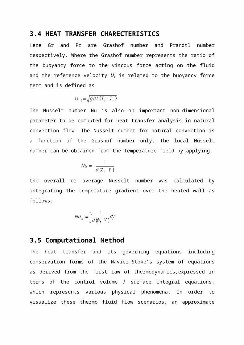
3.4 HEAT TRANSFER CHARECTERISTICSHere Gr and Pr are Grashof number and Prandtl number respectively. Where the Grashof
number represents the ratio of the buoyancy force to the viscous force acting on the fluid and
the reference velocity Uo is related to the buoyancy force term and is defined as

The Nusselt number Nu is also an important non-dimensional parameter to be computed for
heat transfer analysis in natural convection flow. The Nusselt number for natural convection
is a function of the Grashof number only. The local Nusselt number can be obtained from the
temperature field by applying.
the overall or average Nusselt number was calculated by integrating the temperature gradient
over the heated wall as follows:
3.5 Computational MethodThe heat transfer and its governing equations including conservation forms of the Navier-
Stoke’s system of equations as derived from the first law of thermodynamics,expressed in
terms of the control volume / surface integral equations, which represents various physical
phenomena. In order to visualize these thermo fluid flow scenarios, an approximate
numerical solution is need, which can be obtained by the Computational Fluid Dynamics
(CFD) code.
The governing equations of fluid mechanics and convective heat transfer are discretized in
order to obtain a system of approximate algebraic equations, which then can be solved on a
computer. The approximate values are applied to small domain in space and / or time so the
numerical solution provides results at discrete locations in space and time. The accuracy of
the experimental data depends on the quality of the tools used; the accuracy of numerical
solution is dependent on the quality of discretization used. The CFD computation involves
the creation of a set of numbers that constitutes a realistic approximation of a real life system.
The result of the computation work improves the understanding of the behavior of a system.
So, the CFD codes are very useful tools by which engineers can produce physically realistic
result with good accuracy in simulation with finite grids. The broad field of Computational
Fluid Dynamics are the activates that cover the range from the automation of well established
engineering design methods to the use of detailed solution of the Navier-Stokes equations as
substitutes for experimental research into the nature of complex flows. A wide range of fluid
dynamics problems have been solved using CFD codes. CFD codes are more frequently used
in the fields of engineering where the geometry is complicated or some important feature that
can not be dealt with standard methods. The complete Navier-Stokes equations are
considered as the correct mathematical description of the governing equations of fluid
motion. Most of the accurate numerical computation in fluid dynamics comes from solving
the Navier-Stokes equations, since the Navier-Stokes equation represent the conservation of
mass and momentum.
There are five discretization methods available for the high performance numerical
computation of CFD.
* Finite Volume Method (FVM)
* Finite Element Method (FEM)
* Finite Difference Method (FDM)
* Boundary Element Method (BEM)
* Boundary Volume Method (BVM)
The Galerkin Finite Element Method (FEM) is used in this present numerical
computation.
CHAPTER 4
Finite Element Method
4.1 INTRODUCTIONThe Finite Element Method (FEM) is a very powerful computation technique for solving
problems described by ordinary differential equations or partial differential equations. The
Finite Element Method represents an approximate numerical solution of a boundary-value
problem described by ordinary differential equation or partial differential equation.
Differential equation solved by solving the corresponding variation statement of the
differential equation. Variation statements of physical problems usually include some
statement concerning boundary conditions, since boundary condition formulation is a natural
result of variation formulation. The basic concept of the finite element method is that a
continuous function can be approximated using a discrete model. The discrete model is
composed of one or more interpolation polynomials, and the continuous function is divided
into finite pieces called elements. Each element is defined using an interpolation function to
describe the behavior between its end points. The end points of the finite element are called
nodes.
4.1.1 SHAPE FUNCTIONS
The shape function is usually denoted by the letter N and is usually the coefficient that
appears in the interpolation polynomial. A shape function is written for each individual node
of a finite element and has the property that its magnitude is 1 at that node and 0 for all other
nodes in that element.
4.1.2 STIFFNESS MATRIX
The matrix relation between temperature and heat flux is called the stiffness matrix, stiffness
matrix originates from structural analysis. It can be used in others applications in physical
problems. In FEM there are two types of stiffness matrices:
(i) Local stiffness matrix, (ii) Global stiffness matrix
The local stiffness matrix corresponds to individual element. The Global stiffness matrix is
the assemblage of all local stiffness matrices and defines the stiffness of the entire system.
4.2 THE BASIC PRINCIPLE The basic principle of the finite element method is that the domain is broken into a set of
finite elements those are generally triangular or quadrilaterals. The unique feature of FEM is
that the equations are multiplied by a weight function before they are integrated over the
entire domain of the system. In FEM, the solution is approximated by a linear shape function
within each element in a way that guarantees continuity of the solution across elements
boundaries. Such shape function can be constructed from it’s values at the corners of the
elements. The weight function may be the same or different from shape function. This
approximation is then substituted into the weighted integral of the conservation law and the
equation to be solved are derived by requiring the derivative of the integral with respect to
each nodal value to be zero; this corresponds to selecting the best solution within the set of
allowed functions. The obtained result is a set of non-linear algebraic equations.
Mathematical model of physical phenomena may be ordinary or partial differential equations,
which have been the subject of analytical and numerical investigations. The obtained
analytical solutions of these equations involve closed form expressions that give us the
variation of the dependent variables continuously through out the domain. Numerical method
gives approximate solution of these differential equations. At first one has to use a
discretization technique that approximates the differential equation by a system of algebraic
equations at only discrete points in the domain, which can then be solved using a computer
software. To do this, each component of the differential equation is transformed into a
“numerical analogue” which can be represented in the computer and then processed by a
computer program, built on same algorithm. Many different methodologies were devised for
this purpose in the past and the development still continues. In the present thesis the finite
element method (FEM) has been used to solve the differential equations.
4.3 IMPORTANCE OF FINITE ELEMENT METHODThe investigation of flow and heat transfer in thermodynamics can be performed either the
critically or by experimental means. Experimental investigations of such problem could not
gain much acceptance in the field of thermodynamics, because of their limited flexibility and
applications. For each change of geometry of body and boundary condition, it needs separate
investigation, involving separate experimental requirement / arrangement, which in turn make
it unattractive, especially from the time involved as well as economical point of views. On
the other hand, the theoretical investigation can be carried out either by analytical approach
or by numerical approach. Here the analytical techniques of solution are not of much help in
solving the practical problems. Because, it involved a large number of variables, complex
geometrical bodies, boundary conditions and arbitrary boundary shapes. General closed form
solutions can be obtained only for very ideal cases and the results obtained only for very ideal
cases and the results obtained for a particular problem, usually for uniform boundary
conditions. Mathematical model involve partial differential equations are required to be
solved simultaneously with some boundary conditions. So there are no alternatives except the
numerical techniques for the solution of the problem of practical interest. The most useful
numerical methods are the Finite Difference (FD) Method, Finite Volume (FV) Method and
Finite Element (FE) method.
Finite element method is a better numerical approach for solving a system of partial
differential equations. This method produces equations for each element independently of all
other elements. When the equations are collected together and assembled into a global matrix
then the interactions between elements taken into account. Beside these characteristics, the
finite element method dominates in most of computational fluid dynamics. This research

work is an attempt to bring the FE technique again into light through a novel formulation of
two dimensional incompressible thermal flow problems. The philosophy and approach of
these three methods are mentioned here in brief. The finite difference method relies on the
philosophy that the body is in one single piece but the parameters are evaluated only at some
selected points within the body, satisfying the governing differential equations
approximately, where as the finite volume method relies on the philosophy that the body is
divided into a finite number of control volumes, but, in the finite element method, the body is
divided into a number of elements. The comparative merits and demerits of the finite element
method are shown below:
4.4 MERITS AND DEMERITS OF FEM
MERITS OF FEM
1) Finite element method can work though all other methods fail.
2) It is very good in solving complex geometrical bodies and boundaries.
3) There are many commercial packages such as ANSYS,
FEMLAB for analyzing practical problems.
DEMERITS OF FEM
1) The body is not in one piece, but it is an assemblage of elements connected only at nodes.
2) Variations of parameters over individual elements are assumed to be simple like
polynomial of limited order.
3) Finite element solution is highly dependent on the element type.
The accurate and reliable prediction of complex geometry is of great importance to meet the
severe demand reliability and also the economic challenge. This complex geometry occurs
most frequently in computational Fluid Dynamics. The above-mentioned methods have a
common feature; they generate equations for the values of the unknown functions at a finite
number of points in the computational domain. But there are also some differences in them.
The finite difference method and the F. V. M. both generate numerical equations at the
reference point based on the values neighboring points. The finite element method uses the
boundary conditions of Neumann type while the other two methods can use the Dirichlet
conditions. The finite difference method could be extended to multidimensional spatial

domains if the chosen grid is regular. That is the cells must look cuboids, in a topological
sense. Here the grid indexing is simple with some difficulties appear for the domain with a
complex geometry. Where as the finite element method has no restriction on the connection
of the elements when the sides faces of the elements are correctly aligned and have the some
nodes for the neighboring elements. So FEM allows us to model a very complex geometry.
The finite volume method also allows us to model irregular grids like those of the finite
element methods, but keeps the simplicity of writing the equations like that for the finite
different method. Here, it is mentioned that the presence of a complex geometry slows down
the computational programs. Another advantage of the finite element methods is that of the
specific mode to deduce the equations for each element that are then assembled. Thus, the
addition of new elements by refinement of the existing ones is not a major problem. While,
for the other methods, the refinement is a major task and could involve the rewriting of the
program. Though for all the methods used to discretize the initial equation the obtained
system of simultaneous equations must be solved. For this reason, the present work
emphasizes the use of finite element methods to solve flow and heat transfer problems. More
characteristics of this method are explained in the following section.
4.5 USES OF FEM FOR VISCOUS INCOMPRESSIBLE FLOWThis investigation is about on viscous incompressible thermal flows. In this case the problem
is relatively complex due to the coupling between the energy equation and the Navier-Stokes
equations, which govern the fluid flow. These equations consists a set of coupled non-linear
partial differential equations that is difficult to solve especially with complicated geometries
and boundary conditions. The finite element method is one of the computational techniques
that have received popularity because of it’s capability for solving complex structural
problems. This method has been extended to solve problems in several other fields such as in
the field of heat transfer, computational fluid dynamics, electromagnetic, biomechanics etc.
Beside these great success of the method in these fields, convective viscous flows, are still
under intensive research. It is possible due to the fact that the governing of several coupled
equations that are naturally non-linear. It is required a vast amount of computer time and data
storage to find accurate solution. To minimize the computing time and data storage it is used
to employ an adapting meshing technique. The technique sets small elements in the regions
of large change in the solution gradient to increase accuracy of the solution and and large
elements can be used in the other regions to reduce the computational time and computer
memory.
Using the adapting meshing techniques for accurate flow solution, this chapter develops a
finite element formulation that suitable for analysis of general viscous incompressible
thermal flow problems. The derived formula of this chapter will be used with the adaptive
meshing technique in the future. It is required to start with Navier-Stokes equations together
with the energy equation to derive the corresponding finite elements equations.
The computational technique used in the development of the computer program is described
below. The main steps involved in finite element analysis of a typical problem are:
* Generating Mesh (finite elements) by discrimination of the domain.
* Weighted-integral or weak formulation of the differential equation to be analyzed.
* To develop the finite element model of the problem using its weighted-integral or weak
form.
* To assemble the finite elements to obtain the global system of algebraic equations.
* To set the boundary conditions.
* To solve the equation.
* To do the post computation of solution and quantities of interest.
4.6 NUMERICAL TECHNIQUEThe numerical technique used to solve the governing equation for the present work is based
on the Galerkin-Weighted residual method of finite-element formulation. The non-linear
parametric solution method is selected to solve the governing equation. This procedure will
result in substantially fast convergence assurance. In the present investigation a non-uniform
triangular mesh arrangement is implemented in the present investigation especially near the
walls to capture the rapid changes in the development variables.
An iterative scheme is adopted to discretize the velocity and heat energy equation (3.5)-(3.8)
into a set of non-linear coupled equations. For the convergence of the numerical algorithm
the following criteria is applied to all dependent variables over the solution domain.
∑|φijm−φij
m−1|≤10−5
Where represents a dependent variables U, V, P and T; the indexes i, j indicate a grid point;
and the index m is the current iteration at the grid level. For the development of finite element

equation, the six node triangular element is used in this research work. All these six nodes are
involved with velocities and temperature simultaneously, while only the corner nodes are
associated will pressure. For this, a lower order polynomial is chosen for pressure which is
satisfied through continuity equation. In the differential equation
(3.5) (3.8) the velocity component and the temperature distributions and linear interpolation
for the pressure distribution according to their highest order derivatives are as
U (X , Y )=Nα Uα =N1U1+N2U2+N3U3+N4U4+N5U5+N6U6 (4.1)
V (X , Y )=N α V α =N1V1+N2V2+N3V3+N4V4+N5V5+N6V6 (4.2)
θ( X , Y )=Nα θα =N1 V 1+N2 V2+N3 V3+N4V4+N5V5+N6V6 (4.3)
P(X , Y )=H λ Pλ=H1P1+H2P2+H3P3 (4.4)
where α=1 , 2 , ⋯⋯, 6 ; λ=1 , 2 , 3 ; Nα are the quadratic shape functions for the
velocity components and the temperature and H λ are the linear shape functions
for the pressure.
The method of weighted residuals (Zienkiewicz, 1991) is applied to the continuity equation
(3.5), the momentum equations (3.6)(3.7) and the energy equation (3.8), we get
(4.5)
+ 1√Gr∫A
N α(∂2U∂ X2 +
∂2U∂Y 2 ) dA+∫
AN α(sin φ ) θ dA
(4.6)
+ 1√Gr∫A
N α(∂2 U∂ X2 +
∂2V∂Y 2 ) dA+∫
AN α(cosφ ) θ dA
(4.7)
∫A
N α(U ∂θ∂X
+V ∂θ∂Y ) dA= 1
Pr √Gr ∫AN α( ∂2 θ
∂ X2 +∂2θ∂Y 2 ) dA
(4.8)
where A is the element area. Then to generate the boundary integral terms associate with the
surface tractions and heat flux Gauss’s theorem is applied to equation. (4.6)(4.8). The
equations (4.6)(4.8) become,

−∫A
sin φ N αθ dA=∫S0
N α Sx d S0⋯⋯(4.9)
−∫A
cos φ N α θ dA=∫S0
Nα S y d S0⋯⋯(4.10)
∫A
N α(U ∂θ∂X
+V ∂θ∂Y ) dA+ 1
Pr√Gr ∫A (∂Nα
∂ X∂ θ∂ X
+∂ Nα
∂Y∂θ∂Y ) dA
=∫S0
N α qw d Sw⋯⋯(4.11)
Where equation (4.6)(4.7) indicating surface tractions (Sx , S y ) along outflow boundary S0
and (4.8)indicating velocity components and fluid temperature or heat flux that flows into or
out from domain along wall boundary Sw. By substituting the element velocity component
distribution, the temperature distribution and the pressure distribution from equations
(4.1)(4.4), the finite element equations can be written in the form
Kαβ×U β+Kαβ×V β=0 (4.12)
Kαβν xU β U ν+K αβν yV ν U ν+M αμ x Pμ+1
√Gr (Sαβ xx+Sαβ yy ) U β
−sin φK αβ θβ=Qα u (4.13)
Kαβν xU β V ν+K αβν yV ν V ν+Mαμ yPμ+1
√Gr (Sαβ xx+Sαβ yy ) U β
−cos φKαβ θβ=Qα v (4.14)
Kαβν xU β θν+Kαβν yV β θν+1
Pr √Gr (Sαβ xx+Sαβ yy ) U β=Qα ν(4.15)
where the coefficients in element matrices are in the form of the integrals over the element
area and along the element edges So and Sw as below,
Kαβ x=∫A
N α N β , x dA(4.16a)

Kαβ y=∫A
Nα N β , y dA(4.16b)
Kαβν x=∫A
N α N β Nν ,x dA(4.16c)
Kαβν y=∫A
N α N β N ν , x dA(4.16d)
Kαβ=∫A
Nα N β dA(4.16e)
Kαβ xx=∫A
N α , x N β ,x dA(4.16f)
Kαβ yy=∫A
Nα , y N β , y dA(4.16g)
Kαμ x=∫A
Hα H μ , x dA(4.16h)
Kαμ y=∫A
H α Hμ , y dA(4.16i)
Qα u=∫So
Nα Sx dSo
(4.16j)
Qα v=∫So
Nα S y dSo
(4.16k)
Qα θ=∫Sw
Nα qw dSw
(4.16l)
The above element matrices are evaluated in closed form to ready for numerical simulation.
The details calculation for these element matrices are omitted here.
The above finite element equations, equation (4.12)( 4.15), are non-linear which are solved
by applying the Newton-Raphson iteration technique (Dechaumphai, 1999) by first writing
the unbalanced values from the set of the finite element equation (4.12)( 4.15), as below,
FαP=Kαβ xU β+Kαβ yV β (4.17a)
Fα u=K αβν xU β U ν+Kαβν yV νU ν+Mαμ xPμ
+ 1√Gr (Sαβ xx+Sαβ yy ) U β=sin φKαβ θβ−Q
α y
(4.17b)

Fα v=Kαβν xU β U ν+Kαβν yV ν V ν+M αμ yPμ
+ 1√Gr (Sαβ xx+Sαβ yy ) U β=sin φKαβ θβ−Q
αv
(4.17c)
Fα ν=Kαβν xU β θν+Kαβν yV β θν
+ 1Pr√Gr (Sαβ xx+Sαβ yy ) θβ−Q
αν
(4.17d)
The above equation leads to a set of algebraic questions with the incremental unknowns of
the element nodal velocity components, temperatures and pressure in the form below,
[Kuu Kuv Kuθ Kup
K vu K vv Kvθ K vp
K νu K θv Kθθ 0K pu K pv 0 0 ] {Δ u
Δ vΔ θΔ p
}=− {Fαu
Fαv
FαθF βp
}(4.18)
Where
Kuu=Kαβνx U ν +K
ανβx U ν+Kαβν yU β+
1√Gr (Sαβ xx+S
αβ yy )
Kuv=K
αβν yU ν
Kuθ=−sin φKαβ
Kup=Mαμ x
K vu=Kαβμ x V ν
Kuθ=Kαβνx U β+K
ανβ y U ν+1
√Gr (Sαβ xx+Sαβ yy )
Kαθ=−cos φK 2 β
K vp=Mαμ y
Kθu=Kαβνx θν
Kθu=Kαβνx θν
Kθθ=Kαβνx U β+K
αβνy V ν +1
Pr √Gr (Sαβxx+Sαβ yy )
Kθp=0 , K pu=Kαβx , K pv=K
αβ y And K pθ=0=K pp .

Physical Model
Governing Equation
Boundary Condition
Mesh Generation
Start
Forming 6 6 matrix against element
Initial Guess Valuesu*, v*, T*
Assemble All elements
Matrix Factorization
Convergence
u, v, T
Yes
No
The above iteration process is terminated if the percentage of the overall change compared to
the previous iteration is less than the specified value. The Newton-Raphson iteration
technique has been adapted through PDE solver with MATLAB interface to save the sets of
the global non-linear algebraic equations in the form of matrix.
FLOW-CHART OF THE ALGORITHM
4.7 SOLUTION PROCEDURE OF SYSTEM OF EQUATIONSThe obtained result of discretization is a system of linear algebraic equations. This system of
linear algebraic equations has been solved by the UMFPACK with MATLAB interface.
UMFPACK is a set of routines for solving asymmetric sparse linear system of equations
using the Asymmetric Multi Frontal method and direct sparse L.U. factorization. To factorize
A or Ax = b the following five primary UMFPACK routines are required.
1. Pre-orders the columns of A to reduce fill-in and performs a symbolic analysis.
2. Scales Numerically and then factorizes a sparse matrix.
3. To solves a sparse linear system using the numeric factorization.
4. To frees the symbolic object
5. To free the numeric object
Additional routines are:
1. To pass a different column ordering.
2. To change the default parameters.
3. To manipulate sparse matrices.
4. To get L. U. factors.
5. To solve L. U. factors.
6. To compute determinant.
Where UMFPACK factorizes PAC, PRAG or Pr1AQ into the product LU. Here L and U are
lower and upper triangular matrices respectively, P and Q are permutation matrices and R is a
diagonal matrix of row scaling factors, when row-scaling is not used then R = 1. P and Q
are chosen to reduce fill-in with new non-zeros in L and U that are not present in A. The
permutation P has the dual role of reducing fill-in and maintaining numerical accuracy
through relaxed partial pouting and row interchanges. Here the sparse matrix A can be square
or rectangular, singular or non-singular and real or complex or any combination. To solve the
system Ax = b can be solved using only square matrices A. Rectangular matrices can only be
0 2500 5000 7500 10000 12500 15000 17500
5.979
5.98
5.981
5.982
5.983
5.984
1040
4160 10365 12413
13490
14680
16640
factorized. UMFPACK first finds a column pre-ordering that reduces fill-in without regard to
numerical values. This process scales and analyzes the matrix and then one of the three
strategies for pre-ordering the row and columns is selected: asymmetric, 22 and symmetric.
These strategies are given below.
One of the main characteristics of the UMFPACK is that whenever a matrix is factored, the
factorization is stored as a part of the original matrix so that further operation on the matrix
can reuse this factorization. When a factorization or decomposition is done, it is preserved as
a list of elements in the factor slot of the original object. Thus a sequence of operations, such
as determining the condition, number of a matrix and then solving a linear system based on
the matrix, do not require multiple factorizations of intermediate results.
Theoretically, the simplest representation of a sparse matrix is a triplet of an integer vector i
giving the row number, an integer vector j giving the column numbers and a numeric vector x
giving the non-zero values in the matrix. This triplet representation is row-oriented if
elements in the same row were adjacent and column-oriented if elements in the same column
were adjacent. This compressed sparse row or compressed sparse column representation is
similar to row-oriented triplet or column-oriented triplet respectively. The redundant row and
column in indices are removed by these compressed representations and faster access to a
given location in the matrix is obtained.
4.8 GRID INDEPENDENCE TEST The primary results are obtained to inspect the field variables grid independency solutions.
To find out the optimum grid number, the test of accuracy of grid fitness has been carried out.

Figure 4.2: Grid Independence test.
To obtain grid independent solution, a grid refinement study is performed for a rectangular
open cavity with Gr=106 and dr=0.2.The above figure shows the convergence of the average
Nusselt number, Nu at the heated surface with grid refinement. It is observed that grid
independence is achieved with 13686 elements where there is insignificant change in Nu with
further increase of mesh elements. The grid refinement tests are done by taking six different
non –uniform grids with the following number of nodes and elements : 27342 nodes,4818
elements; 49335 nodes, 7663 elements;72782 nodes,10365 elements;73542 nodes, 11413
elements; 96030 nodes, 12356 elements; 892450 nodes, 13686 elements. In this case
982450 nodes, 13686 elements can be chosen through the processing to optimize the relation
between the accuracy required and the computational time.
4.9 MESH GENERATIONThe Mesh generation is the technique to subdivide a domain into a set of Sub-domains,
called finite elements. Figure 4.3 shows a domain A is subdivided
into a set of sub domains , Ac with boundary
Figure 4.3: Finite element mesh of the solution domain
Here the numerical technique will discretize the computational domain into unstructured
triangles by Delaunay Triangular method. The Delaunay triangulation is a geometric structure
that has enjoyed great popularity in mesh generation since the initial age of mesh
generation technique .The Delaunay triangulation of a vertex set maximizes the minimum
angle among all possible triangulations of that vertex set .
Figure 4.4: Finite element discretization of a domain
The present numerical technique will discretized the computational domain into unstructured triangles
by Delaunay Triangular method. The Delaunay triangulation is a geometric structure that has enjoyed
great popularity in mesh generation since the mesh generation was in its infancy. In two dimensions,
the Delaunay triangulation of a vertex set maximizes the minimum angle among all possible
triangulations of that vertex set.
Figure 4.4: Current mesh structure of elements for rectangular open cavity containing a
heated circular cylinder inside the cavity.
The above figure 4.4 shows that the mesh mode for the present numerical process. Mesh
generation has been done meticulously.
CHAPTER 5
Results and DiscussionsA numerical study has been done on two-dimensional laminar steady state natural convection
flow in a rectangular open cavity with left vertical wall is at a constant heat flux as shown in
Λe

Figure 3.1. A heated circular cylinder is placed at the centre of the cavity. The opposite wall
of the cavity is heated by a constant heat-flux. The bottom and top walls are kept at high and
cool temperature respectively. Using Gelarkin- finite element method two-dimensional
Navier–Stokes equations along with the energy equations are solved .The results are obtained
for Grashof number from 103 to 106 at Pr = 0.72, 1.0 and 7.0 with constant physical
properties. Here the parametric analysis for a wide range of governing parameters shows
consistence performance of the present numerical approach to obtain as stream functions and
temperature profiles.
The obtained results show that the heat transfer coefficient is strongly affected by Grashof
number. An empirical correlation can be developed using Nusselt number and Grashof
number. For high values of Grashof number the errors encountered are appreciable. Hence it
is necessary to perform some grid size testing in order to establish a suitable grid size. Grid
independency is ensured by comparing the results of different grid meshes for Gr=106 which
was the highest Grashof. The total domain is discretized into 4160 elements that result in
6240 nodes; into 3760 elements that result in 5640 nodes, etc.
The effect of inclination angle is examined for = 0o, 15o, 30o,45o with aspect ratio A=1. A
comparative study between the steady state patterns of streamlines from Grashof numbers of
103 to 106 with different angles is presented in figures 5.1 to 5.20
Simultaneously a comparison between the steady- state patterns of isotherms from Grashof
numbers from 103 to 106 with different angles is presented in figure 5.1 to 5.20. The isotherm
figures show that as the Grashof number and the inclination angle increases, the buoyancy
force increases and the thermal boundary layers become thinner. The figures of streamlines
show that the fluid enters from the left wall of the aperture, circulates in a clockwise direction
following the shape of the cavity and leaves toward the upper part of the aperture. The
streamlines patterns is very similar for first one Grashof number and the inclination angle, but
the fluid moves faster for G=104. Similar streamline patterns raised for Gr=105 and 106 but the
upper boundary layer becomes thinner and faster, the velocity of the air flow moving toward
the aperture increases and the area occupied by hot fluid decreases in comparison of the
entering fluid. Streamlines and Isotherms show that as the inclination angle of the heated wall
increases, the velocity gradient remained almost same as before.

The results are also presented in terms of streamlines and isotherm patterns. The variations of
the average Nusselt number and the average temperature are also presented. The results in the
steady state are obtained for a Grashof numbers ranging from 103 to 106 and for inclination
angles range from 0o to 45o of the cavity.
Table 5.1 Results for the same surface temperature with Pr=0.72
Gr Nuav
Present work Hinojosa et al.(2005)103
104
105
106
1.35
3.55
7.50
14.62
1.30
3.44
7.44
14.51
5.1 EFFECTS OF INCLINATION ANGLEDue to increase of the Grashof number complex flow pattern characteristics were found for
various inclination angles. This profile of streamlines, isotherms and inclination angles of the
cavity 0o, 15o, 30o and 45o are presented in Fig. 5.1 to 5.19.The steady state can be reached for
inclination angles of the cavity between 0o and 45o. The average Nusselt number for different
cavity’s inclination angles and Grashof numbers for Prandtl number Pr = 0.72 and dr = 0.2 is
presented .The average Nusselt numbers for four Grashof numbers (103,104,105and 106) for a
range of 0o to 45o presented in table 5.2 for tilted angles of the open cavity. The average
Nusselt number increases mainly for higher angles and for higher Grashof number.
Hence, in Table 5.2 the average Nusselt number and their standard deviation are reported. It
is observed that the heat transfer rate Nu increases with the increases of inclination angle
and increase of Grashof number.
Table 5.2 shows the Average Nusselt number Nu for different cavity’s inclination angles
and Grashof numbers for Pr = 0.72 and dr = 0.2.
Nuav
Gr=103 Gr=104 Gr=105 Gr=106
0o 3.2725 3.29 4.07 5.494715o 3.2756 3.37 4.2837 5.8547

30o 3.3525 3.5443 4.5646 5.965745o 3.4125 3.4956 4.7543 5.9757
5.2 EFFECTS OF PRANDTL NUMBERThe effects of Prandtl number on the flow and heat transfer characteristics, a study for
Pr = 0.72, 1.0 and 7.0 is investigated. The predicted streamlines and isotherms are in Figure
5.1 to 5.19. It is observed that fluid moves clockwise around the cylinder.
Average Nusselt numbers are determined for different Prandtl numbers: Pr =0.72, 1.0 and 7.0
and Grashof numbers are obtained with the present nodal for angle = 0o and diameter ratio
dr=0.2 is presented.
The streamlines for dr =0.2 ,Pr = 0.72, Th=320k and for inclination angles = 0o ,15o, 30o,
45o are shown in Fig. 5.1 to 5.4 for variation of Grashof number Gr .For Gr = 103 , 105
the streamlines are almost laminer but one and two vortexes are created for Gr =104 and 106
respectively.
The streamlines for dr =0.2 , Pr =1.0 ,Th =320 k and for inclination angles = 0o ,15o , 30o
45o are shown in Fig 5.5 to 5.8 for the variation of Grashof number. For Grashof number
103, 105 the streamlines are almost laminer but one and two vortexes are created for
Gr = 104 and 106 respectively. The streamlines for dr =0.2 , Pr = 7.0 ,Th =320 k and for
inclination angles = 0o ,15o , 30o 45o are shown in Fig 5.9 to 5.12 for the variation of
Grashof number. For Grashof number 103 ,the streamlines are almost laminar but two
voetexes are created for Gr =104 near the left wall and heated cylinder respectively for Gr
=104 .Two recirculation cells are created one near left wall and one near the cylinder
respectively for Gr = 105 . Two large recirculations are formed ,one is near left wall and one
is near the cylinder for Gr =106.
The streamlines for dr =0.2 , Pr =1.0 ,Th =350 k and for inclination angles = 0o ,15o , 30o
45o are shown in Fig 5.13 to 5.15 for the variation of Grashof number. For Grashof
number103,the streamlines are almost laminer but one vortexe is created for
each of Gr = 104 , 105and 106 respectively near the cylinder , one small vortex is formed
near the bottom wall at = 0o.
For = 15o and Th =350k: For Gr = 103 streamlines are laminar ,but one vortex is formed
for each of Gr =104,105 . For Gr =106 two recirculation cells and one vortexes are formed
near the cylinder .
For = 30o and Th =350k: For Gr = 103 streamlines are laminar ,but one vortex is formed
for each of Gr =104,105 . For Gr =106 two recirculation cells and one vortexes are formed
near the cylinder .
The streamlines for dr =0.2 , Pr =1.0 ,Th =375 k and for inclination angles = 0o ,15o , 30o
45o are shown in Fig 5.16 to 5.19 for the variation of Grashof number. For Grashof
number103,the streamlines are almost laminer but one vortexe is created for
each of Gr = 104 , 105 ; but two recirculations are formed near the cylinder and bottom wall
for Gr = 106 .
The streamlines for dr =0.2 , Pr =1.0 ,Th =375 k and for inclination angles = 0o ,15o , 30o
45o are shown in Fig 5.16 to 5.19 for the variation of Grashof number. For Grashof
number103,the streamlines are almost laminer but one vortexe is created for
each of Gr = 104 , 105 ; but two recirculation cells are formed near the cylinder and bottom
wall for Gr = 106 .
The results show that insignificant difference for different angles. Heat transfer
characteristics become low for lower Prandtl number Pr =.72 and high for higher Prandtl
number. Heat transfer is higher than that in the case Pr =7.0 have a lower thermal diffusitivity
than that of the fluid with Pr = 0.72.
So the fluid with Pr =7.0 will tend to exchange less heat with surrounding fluid by diffusion.
Table 5.3: Average Nusselt numbers for different Prandtl number taking Pr = 0.72, 1.0
and 7.0, angle =0o and dr =0.2
Nuav
Pr Gr =103 Gr=104 Gr =105 Gr=106
0.72 3.282456 3.297536 4.257526 5.674695
1.0 3.273425 3.359545 4.346528 5.885685
7.0 3.325456 4.423145 4.875256 8.844667

Gr=
103
Gr=
104
Gr=
105
Gr=
106
Streamline Isotherm
Fig. 5.1 Streamlines and isotherms for dr =0.2 and Pr =0.72 at an angle 0o taking Th =320k

Fig 5.2: Streamlines and isotherms patterns for dr = 0.2 and Pr = 0.72 at angle 15o
Gr =
104
Gr =
103
Gr =
105
Gr =
106

Gr=
103
Gr =
104
Gr =
105
Gr=
106
Streamlines Isotherms
Fig 5 .3 : Streamlines and Isotherms patterns for dr = 0.2 and Pr =0.72 atangle30o

Gr =
103
Gr=
104
Gr =
105
Gr=
106
Streamline IsothermFig5.4: Isotherms and streamlines patterns for dr = 0.2 and Pr = 0.72 at angle 45o
and Th=320k

Gr=
103
Gr=
104
Gr=
105
Gr=
106
Fig.5.5: Streamlines and isotherms for dr =0.2,Pr = 1 at an angle 0o taking Th=320k,Tc=276k
Gr=
103
Gr=
104
Gr=
105

Gr=
106
Streamline Isotherm Fig.5.6: Streamline and isotherm patterns for dr =0.2 and Pr = 1 at an angle 15o ,Th =320k
Gr=
103
Gr=
104
Gr=
105

Gr=
106
Streamlines Isotherms
Fig. 5.7 Streamlines and isotherms for dr = 0.2 and Pr =1 at an angle 30o,Th =320k, Tc=276
Gr=
103
Gr=
104
Gr=
105
Gr=
106
Streamline Isotherm Fig. 5.8 Streamlines and isotherms for dr = 0.2 and Pr =1 at an angle 45o,Th =320k, Tc=276
Fig. 5.9 Streamlines and isotherms for dr=0.2 and Pr=7 at an angle 0o , taking Th =320k
Gr =
103

Gr =
104
Gr =
105
Gr =
106
Streamlines Isotherms
Gr =
103

Gr =
104
Gr =
105
Gr =
106
Streamlines IsothermsFig. 5.10 : Streamlines and isotherms patterns for dr =0.2 and Pr =7 at an angle 15o,Th =320k

Gr=
103
Gr=
104
Gr=
105

Gr=
106
Streamline Isotherms
Fig.5.11: Streamlines and isotherms patterns for dr =0.2 and Pr =7.0 at an angle 30o, taking Th =320k
Gr=
103

Gr=
104
Gr=
105
Gr=
106
Streamline Isotherm
Fig. 5.12: Streamlines and isotherms for dr =0.2 and Pr = 7 at an angle 45o, Th= 320k

Gr=
103
Gr=
104
Gr=
105

Gr=
106
Streamline IsothermFig. 5.13 Streamlines and isotherms for dr = 0.2 and Pr =1 at an angle 0o, Th =350k,Tc=278k
Gr=
103
Gr=
104

Gr=
105
Gr=
106
Streamline IsothermFig .5.14 Streamlines and isotherms for dr =0.2 and Pr =1 at an angle 15o ,Th =350k
Gr =
103
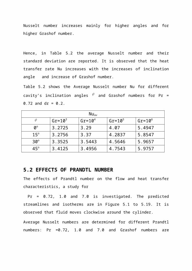
Gr =
104
Gr =
105
Gr =
106
Streamlines IsothermsFig5.15 Streamlines and isotherms pattern for dr =0.2 and Pr =1 at an angle 30o ,Th=350k
Gr =
103

Fig. 5.16: Streamlines and isotherms for dr = 0.2 and Pr =1 at an angle 0o, Th =375k
Gr =
103
Gr =
104
Gr =
105
Gr =
106

Fig. 5.17: Streamlines and isotherms for dr =0.2 and Pr =1 at an angle15o with Th= 375k
Gr =
103
Gr =
105
Gr =
106
Gr =
104

Fig. 5.18: Streamlines and isotherms for dr =0.2 and Pr =1 at an angle 30o,Th =375k
Streamlines Isotherms
Gr =
104
Gr =
105
Gr =
106
Gr =
103

Fig 5.19 Streamlines and isotherms for dr=0.2 and Pr=1 at an angle 45o ,Th =375k
Gr =
106
Gr =
105
Gr =
104

Gr
Nu
103 104 105 106
15
20
25
30
35
40
45
Fig.5.20.: Variation of average Nusselt number against Grashof number for different inclination angles while Pr = 0.72, dr = 0.2.
Gr
Nu
103 104 105 106
15
20
25
30
35
40
45
Fig.5.21.: Variation of average Nusselt number against Grashof number for different inclination angles while Pr = 1.0, dr = 0.2.

Gr
Nu
103 104 105 1060
50
100
150
200
250
300
350
400
Fig.5.22.: Variation of average Nusselt number against Grashof number for different inclination angles while Pr = 7.0, dr = 0.2.
Gr
Nu
103 104 105 1060
50
100
150
200
250
300
350
400
450
Pr = 0.72Pr = 1.0Pr = 5.0Pr = 7.0
Fig.5.23.: Variation of average Nusselt number against Grashof number for different inclination angles while = 0o , dr = 0.2.
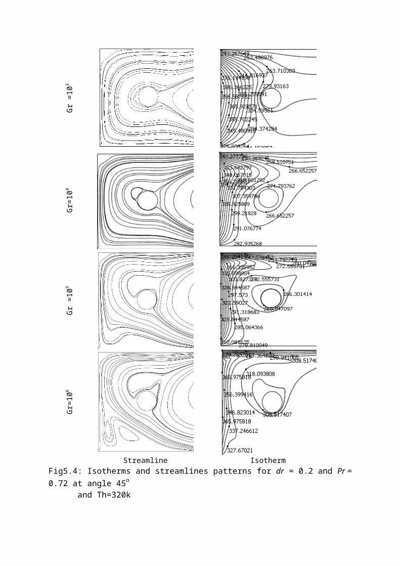
Gr
Nu
103 104 105 106
50
100
150
200
250
300
350Pr = 0.72Pr = 1.0Pr = 5.0Pr = 7.0
Fig.5.24.: Variation of average Nusselt number against Grashof number for different inclination angles while = 15o , dr = 0.2.
Gr
Nu
103 104 105 1060
50
100
150
200
250
300
350Pr = 0.72Pr = 1.0Pr = 5.0Pr = 7.0
Fig.5.25.: Variation of average Nusselt number against Grashof number for different inclination angles while = 30o , dr = 0.2.
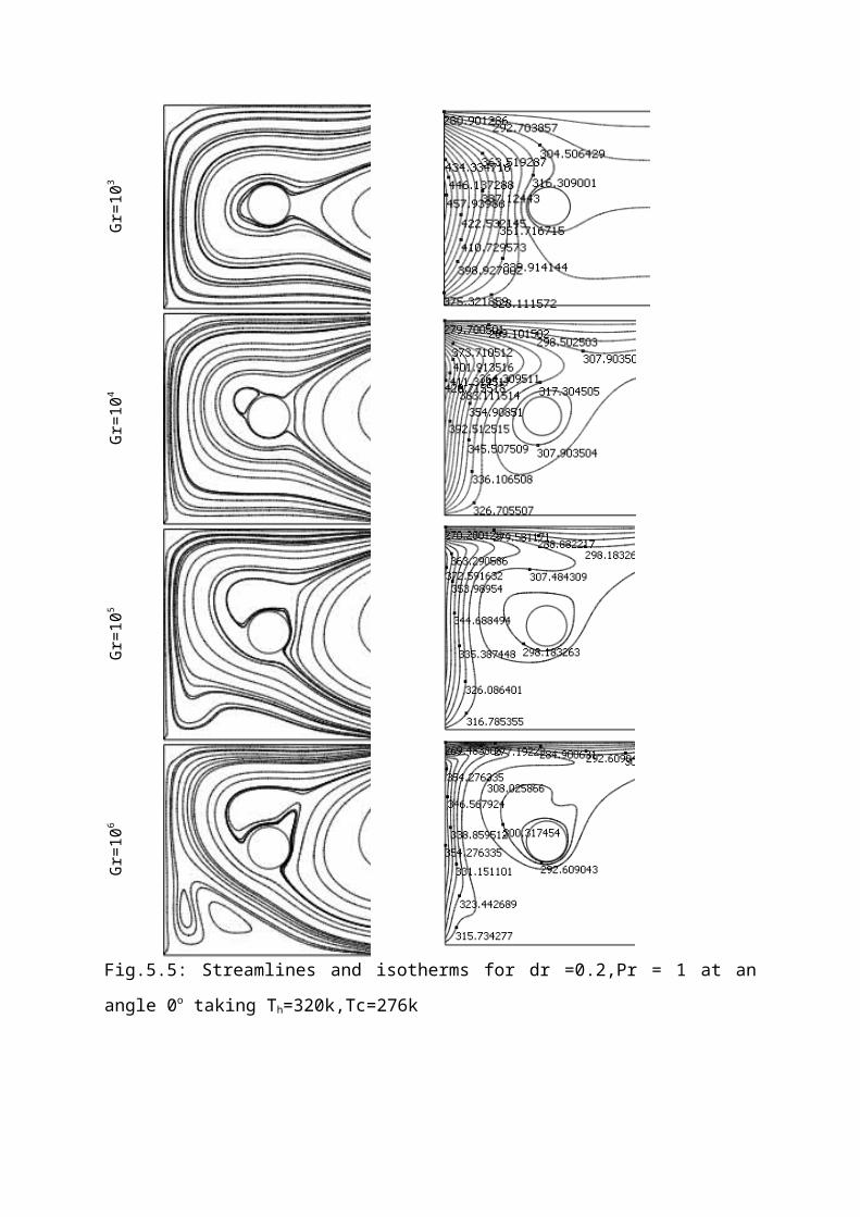
Gr
Nu
103 104 105 1060
50
100
150
200
250
300
350Pr = 0.72Pr = 1.0Pr = 5.0Pr = 7.0
Fig.5.26.: Variation of average Nusselt number against Grashof number for different inclination angles while = 45o , dr = 0.2.
5.3 CONCLUSIONIn this research work two- dimensional laminar steady –state natural convection flow in a
rectangular open cavity with the left vertical wall is at constant heat flux has been studied
numerically. A finite element method is used for a steady state incompressible natural
convection flow. The governing flow equations that consist of the conservation of mass,
momentum and energy equation are discretized to finite element equations. The obtained
finite element equations are nonlinear requiring an iterative technique solver. Solving these
non-linear equations the Newton –Raphson iteration method has applied. The solution of the
nodal velocity component, temperature and pressure by considering Prandtl numbers Pr=
0.72, 1.0 and 7.0 and Grashof numbers from 103 to106. The following characteristics are
found in the work:
Heat transfer rate depends on Prandtl number and heat transfer rate increases as
Prandtl number increases.
Thermal boundary layer thickness becomes thinner for higher Grashof number.
The heat transfer rate decreases for Gr=103 and increases gradually for increasing of
Grashof number.
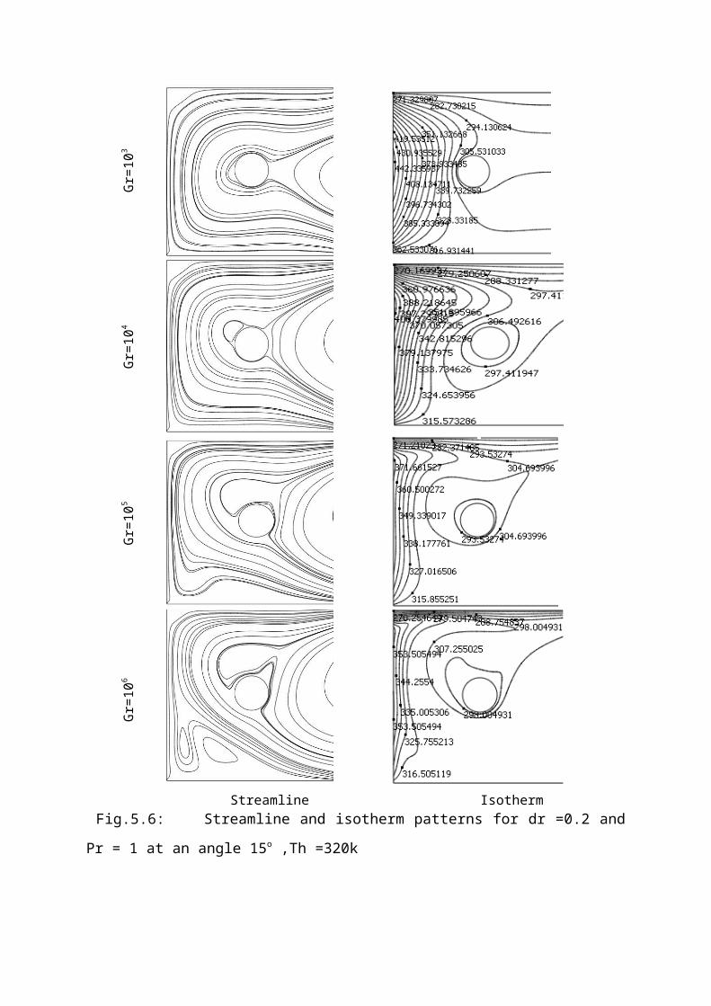
The heat transfer rate Nu increases as inclination angle increases and increases of
Grashof number.
Various vortexes entering into the flow field and a boundary vortex at the centre of
the cavity is seen in the streamlines.
5.4 FUTURE SCOPE OF STUDYIn the present study it is considered that two –dimensional laminar steady-state natural
convection in a square open cavity containing a heated circular cylinder. The circular cylinder
is placed at the centre of the cavity and the left sidewall is heated by constant heat flux. The
top wall is kept at cool temperature while the bottom wall is kept at high temperature.
If we consider a partially heated circular cylinder inside the cavity instead of heated
cylinder then we can extend our work.
Again, taking non-uniform surface temperature the work can be extended.
REFERENCES Arnold, J. N., Catton, I., and Edwards, D. K., “Experimental Investigation of Natural Convection in Inclined Rectangular Regions of Differing Aspect Ratios,” Journal of Heat Transfer, Vol. 98, pp.67-71, 1976.
Bilgen, E., and Oztop, H., “Natural convection heat transfer in partially open inclined square
cavities”, Int. J. of Heat and Mass Transfer, Vol. 48, pp. 1470-1479, 2005a.
Chan,Y. L. and Tien, C. L., “A Numerical study of two-dimensional natural convection in square open cavities”, Numerical Heat Transfer, Vol. 8, pp. 65-80, 1985b.
Chan,Y. L. and Tien, C. L., “A Numerical study of two-dimensional laminar natural convection in a shallow open cavity”, Int. J. Heat Mass Transfer, Vol. 28, pp. 603-612,1985.
Cook, R. D., Malkus, D. S., and Plesha, M. E., “Concepts and applications of finite element analysis”, Third Ed., John Wiley & Sons, New York, 1989.
De, A.K. and Dalal, A.,“A numerical study of natural convection around a square, horizontal, heated cylinder placed in an enclosure”, Int. J. of Heat and Mass Transfer, Vol. 49, pp. 4608-4623, 2006.
Dechaumphai, P., Finite Element Method in Engineering, second Ed., Chulalongkorn University Press, Bangkok, 1999.
Frederick, R. L. “Natural convection in an inclined square enclosure with a partition attached to its cold wall”, Int. J. Heat and Mass Transfer,Vol. 32, pp. 87–94, 1989.

Gallagher, R. H., Simon, B. R., Johnson, P. C. and Gross, J. F., Finite elements in biomechanics, John Wiley & Sons, New York, 1982.
Saha, G., Saha, S. and Mamun, M.A.H., “A Finite Element Method for Steady-State Natural Convection in a Square Tilt Open Cavity”, ARPN Journal of Engineering and Applied Sciences, Vol. 2, No. 2, pp. 41-49, 2007.
Hamady, F. J., Lloyd, J. R., Yang, H. Q., and Yang, K. T., “Study of Local Natural convection Heat Transfer in an Inclined Enclosure,” International Journal of Heat and Mass Transfer, Vol. 32, pp.1697-1708, 1989.
Hinojosa, J. F., Estrada, C. A., Cabanillas, R. E., and Alvarez, G., “Nusselt number for the natural convection and surface thermal radiation in a square tilted open cavity”, Int. Com. In Heat and Mass Transfer, Vol. 32, pp. 1184-1192, 2005.
Jini, J., The finite element method in electromagnetics, John Wiley & Sons, New York, 1993.
Kangni, A., Ben, R. and Bilgen, E. “Natural convection and conduction in enclosure with multiple vertical partitions”, Int. J. Heat and Mass Transfer,Vol. 34, p. 2819–2825, 2003.
Kuhn, D. and Oosthuizen, P. H., “Unsteady natural convection in a partially heated rectangular cavity”, ASME Journal of Heat Transfer, Vol. 109, pp. 789–801, 1987.
Lakhal, E. K., Hasnaoui, M.and Vasseur, P., “Numerical study of transient natural convection in a cavity heated periodically with different types of excitations”, International Journal of Heat and Mass Transfer, Vol. 42, No. 21, pp. 3927–3941, 1999.
Le Quere, P., Humphery, J. A., and Sherman, F.S. ”Numerical calculation of thermally driven two-dimensional unsteady laminar flow in cavities of rectangular cross section”, Numerical Heat Transfer, Vol. 4, pp. 249-283,1981.
Lewis, R.W., Morgan, K., Thomas, H. R. and Seetharamu, K. N., The Finite element method in heat transfer analysis, John Wiley & Sons, New York, 1996.
Linthorst, S.J.M., Schinkel, W. M. M., and Hoogendorn, C. J., “Flow Structure with Natural convection in Inclined Air-filled Enclosures,” Journal of Heat Transfer. Vol. 103, pp.535-539, 1981.
Mohamad, A., “Natural convection in open cavities and slots”, Numerical Heat Transfer, Vol. 27, pp. 705-716, 1995.
Ozoe, H., Sayama, H., and Churchill, S. W., “Natural Circulation in an Inclined Rectangular channel at Various Aspect Ratios and Angles—Experimental Measurements,” International Journal of Heat and Mass Transfer, Vol.18, pp.1425-1420, 1975.
Ozoe, H., Sayama, H., and Churchill, S. W., “Natural Convection in an Inclined Square Channel,” International Journal of Heat and Mass Transfer, Vol. 17, pp.401-406,1974.
P. V. S. N. Murthy, et al “Nutural Convection Heat Transfer from a horizontal wavy surface in a porous enclosure”.J . OF Numerical Heat Transfer , Part-A ,1997 .
Penot, F., “Numerical calculation of two-dimensional natural convection in isothermal open cavities”, Numerical Heat Transfer, Vol. 5, pp. 421-437, 1982.
Peraire, J., Vahidati, M., Morgan, K., and Zienkiewicz, O. C. Adaptive remeshing for compressible flow computation, Journal of Computational Physics, Vol.72, pp. 449-466, 1987.
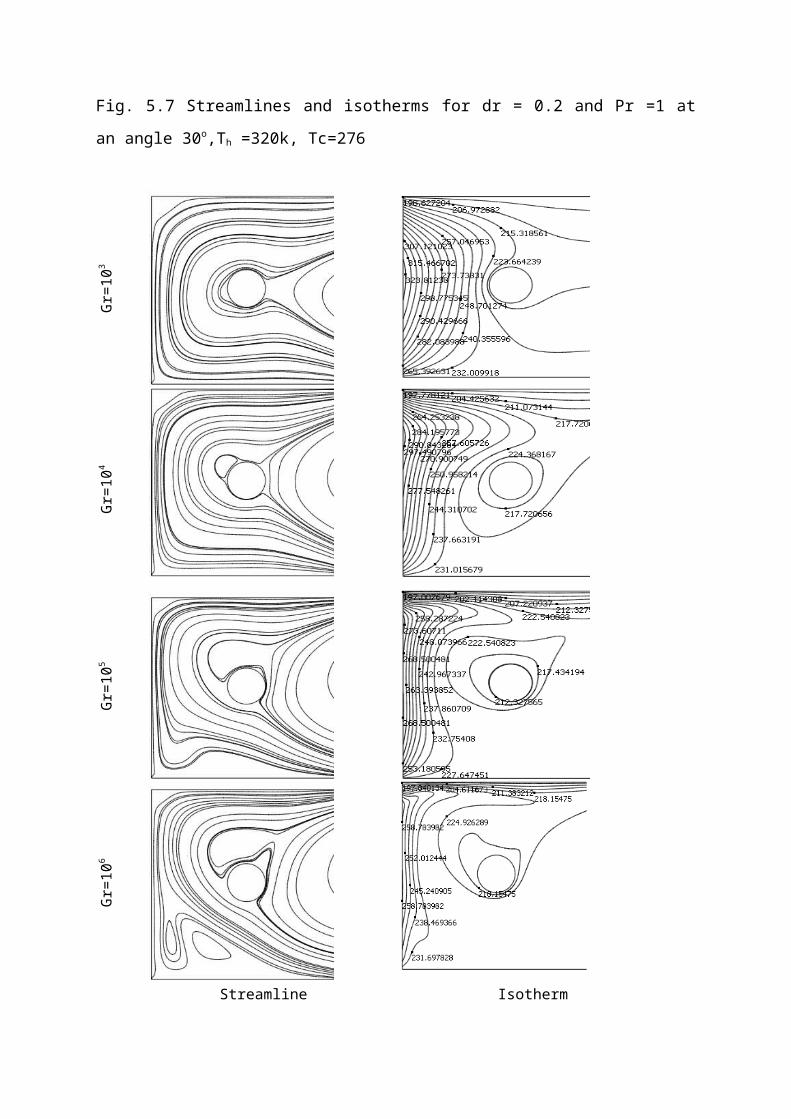
Polat, O. and Bilgen, E. “Laminar natural convection in inclined open shallow cavities”, Int. J. Therm Sci, Vol. 41, pp. 360-368, 2002.
Rahman M. A ,et al , “ Finite Element Analysis of Mixed Convection in a Rectangular Cavity with a Heat –Conducting Horizontal Circular Cylinder”, J . of Non Linear Analysis-2009 vol-14 , no 2.
Showole, R.A. and Tarasuk, J.D., “Experimental and numerical studies of natural convection with flow separation in upward-facing inclined open cavities”, Journal of Heat Transfer, Vol. 115, pp. 592-605, 1993.
Soong, C. Y., Tzeng, P. Y., Chiang, D. C., and Sheu, T. S., “Numerical Study on Mode-transition on Natural Convection in Differentially Heated Inclined Enclosures”, International Journal of Heat and Mass Transfer, Vol. 39, No. 14, pp. 2869-2882, 1996.
Tasnim, S. T. and Collins, M.R. “Numerical analysis of heat transfer in a square cavity with a baffle on the hot wall”, Int. Com. Heat and Mass Transfer, Vol. 31, pp. 639–650, 2004.
Zhao, Y.,“Investigation of Heat Transfer Performance in Fenestration System Based on Finite Element Methods,” Ph.D. Thesis, Department of Mechanical and Industrial Engineering, University of Massachusetts Amherst, 1997.
Zhong, Z.Y., Yang, K. T., and Lloyd, J. R., “Variable-property Natural convection in tilted Enclosures with Thermal Radiation”, Numerical Methods in Heat Transfer, Vol. III, pp. 195-214, 1985.
Zienkiewicz, O. C. and Taylor, R. L. The finite element method, Fourth Ed., McGraw-Hill. 1991.
Fariza Tul Koabra ‘ Numerical investigation on Two-dimensional laminar steady –state natural convection in a rectangular open cavity containing a adiabatic circular cylinder.’ Thesis paper for the degree of M.Phil. in Mathematics, BUET,Dhaka (2008).
Ben-Nakhi, M.M. Eftekhari and D.I. Loveday, ‘Natural Convection Heat Transfer in a partially open Square Cavity with fin attested to the wall’-ASME Journal of Heat Transfer. 2008.