NUMERICAL INVESTIGATION OF THE DECAY RATE OF … · t s ds+ uux= uxx: in the BBM form. In order to realize this numerical study, a numerical scheme based of the ... (s) t s dsstands

INTERNATIONAL JOURNAL OF c© 2013 Institute for ScientificNUMERICAL ANALYSIS AND MODELING Computing and InformationVolume 10, Number 2, Pages 333–349

NUMERICAL INVESTIGATION OF THE DECAY RATE OF

SOLUTIONS TO MODELS FOR WATER WAVES WITH

NONLOCAL VISCOSITY

SERGE DUMONT AND JEAN-BAPTISTE DUVAL

(Communicated by Jie Shen)

Abstract. In this article, we investigate the decay rate of the solutions of two water wave models

with a nonlocal viscous term written in the KdV form

ut + ux + βuxxx +

√ν√π

∫ t

0

ut(s)√t− s

ds+ uux = νuxx.

and

ut + ux − βutxx +

√ν√π

∫ t

0

ut(s)√t− s

ds+ uux = νuxx.

in the BBM form. In order to realize this numerical study, a numerical scheme based of theGα-scheme is developed.

Key words. waterwaves, viscous asymptotical models, long-time asymptotics, fractional deriva-

tives.

1. Introduction

Modeling the effect of viscosity on the gravity waves is a challenging issue andmuch research on this subject has been carried out during last decade. After thepionneer work of Kakutani and Matsuuchi [14], P. Liu and T. Orfila [15], and D.Dutykh and F. Dias [12] have derived, independently, asymptotical models for longgravity waves on viscous shallow water. These models are Boussinesq type systemswith a non local in time viscous terms. A one-way reduction of these models wasadressed in [11].

Computing the decay rate for solutions of that type of problem is also a chal-lenging issue [1, 3, 4, 8]. In a previous work [7], Chen et al. were concerned withcomputing both theoretically and numerically the decay rate of solutions to a waterwave model with a nonlocal viscous dispersive term. This model is the following

(1) ut + ux + βuxxx +

√ν√π

∫ t

0

ut(s)√t− s

ds+ γuux = αuxx,

where u is the horizontal velocity of the fluid. This equation requires some com-ments: the usual diffusion is −αuxx, while βuxxx is the geometric dispersion and√ν√π

∫ t0ut(s)√t−sds stands for the nonlocal diffusive-dispersive term and models the vis-

cosity. Here α, β, γ and ν are non negative parameters dedicated to balance orunbalance the effects of viscosity and dispersion versus the nonlinear effects. Specif-ically the authors have obtained the following global existence and decay results

Received by the editors March 11, 2011 and, in revised form, January 19, 2012.2000 Mathematics Subject Classification. 35Q35, 35Q53, 76B15, 65M70.The authors thank Professor Olivier Goubet for his pertinent remarks. The present work was

initiated when the authors were visiting the Math Department in Purdue University, with the

support of the CNRS for the research exchange program waterwaves.

333

334 S. DUMONT AND J. DUVAL

for the problem (1) with β = 0 (see also [13] for β = 1 and γ = α = 0) with smallinitial datum. More precisely, they state the following theorem.

Theorem 1 (Chen et al., 2009). Consider (1) with β = 0 supplemented withinitial data u0 ∈ L1(R) ∩ L2(R). There exists ε > 0, C(u0) > 0 such thatfor all ‖u0‖L1(R) < ε, there exists a unique global solution u ∈ C(R+;L2

x(R)) ∩C1(R+;H−2

x (R)). In addition, u satisfies

(2) t12 ‖u(t)‖L∞x (R) + t

14 ‖u(t)‖L2

x(R) 6 C(u0)

and u solves the fixed point equation

(3) u(t, x) = K(t, .) ? u0 +N ∗ u2,

where K and N are given by

K(t, x) =1

2√πte−

x2

4t e−x−(

1 +1

2

∫ +∞

0

e−µ2

4t −µ|x|2t −

µ2 dµ

)and

N(t, x) =1

2√πt∂x

[e−

x2

4t −x−(

1− 1

2

∫ +∞

0

e−µ2

4t −µ|x|2t −

µ2 dµ

)],

with x− = max(−x, 0), ? denotes the usual convolution product in space and ∗ thetime-space convolution product defined by

v ∗ w(t, x) =

∫ t

0

∫Rv(s, y)w(t− s, x− y) dx dy

whenever the integrals make sense.

The proof of this theorem can be found in [7].We also consider the following equivalent BBM (Benjamin-Bona-Mahony) form

of the equation (1)

(4) ut + ux − βutxx +

√ν√π

∫ t

0

ut(s)√t− s

ds+ γuux = αuxx.

In this article we investigate the asymptotical decay rate of the solutions withseveral numerical simulations for the two asymptotic models (1) and (4). First, wewill compare our numerical simulations to the results of theorem 1 and those from[7] in order to validate the numerical scheme developed in this article. Then, wewill discuss in the sequel the role of respectively the non local viscous terms, thegeometric dispersion and the nonlinearity.

This article is organized as follows. In the second section, we recall some defi-nitions and give some notations used in this article, such as the Fourier transformand the Gear operator which will be used to approximate the non local viscous

term

√ν√π

∫ t

0

ut(s)√t− s

ds. In section 3, after a presentation of the numerical scheme,

we perform several numerical simulations for equation (1). In the last section, wenumerically analyze the decay rate of the solutions for equations (4) with differentvalues of the parameters (α, β, γ and ν).

2. Some notations and definitions

2.1. Notations. Let us introduce some notations that we shall use in the sequel.The Fourier transform of a function u in L1(R) reads

u(ξ) = F(u)(ξ) =

∫Ru(x) e−ixξ dx.

NUMERICAL STUDY OF WATER WAVE MODELS 335

We expect the decay rate of the solution to be O(ta), with a < 0, namely

||u(t, .)||L2x≈ Cta or ||u(t, .)||L∞x ≈ Ct

a′ for t large, the ratios

R2 =

log

(||u(t+∆t,.)||L2

x

||u(t,.)||L2x

)log( t+∆t

t )and R∞ =

log(||u(t+∆t,.)||L∞x||u(t,.)||L∞x

)log( t+∆t

t )

approach a and a′ as t→∞. Here ∆t denotes the time step. We use, in the sequel,the ratios R2 and R∞ to describe the decay rate of the solutions.

2.2. Outline of the Gα-scheme. In [7], the time dependent equation

(5) ut +

√ν√π

∫ t

0

ut(s)√t− s

ds = f(t), u(t = 0) = u0,

is discretized writting u as a convolution

(6) u(t) = u0 +

∫ t

0

N(ν(t− s))f(s) ds

where N(t) =1√πet∫ +∞

t

e−s√sds. The drawback of this method is that this is

not suitable to approximate the solution of equation (4). Then, we consider in

this article a direct discretization of the half derivative1√π

∫ t

0

ut(s)√t− s

ds using the

Gα-scheme.This method consists in approximating the fractional derivative by an Euler

backward formula and was developed by Galucio et al [9] (see also [10] for moredetails). In order to explain the main ideas of this method, let u be a time dependentfunction, and consider only its discretized values un at each time tn = n∆t wheren is a positive integer and ∆t is the time step, supposed to be fixed. Let G be theGear operator that approximates the first derivative of u, defined by

(7) G =1

∆t

[3

2I − 2δ− +

1

2(δ−)2

]where the backward operator δ is defined by

(δ−u)n = un−1.

Thus we can formally approximate the α-derivative of u by the formula

(8) Gα =1

∆tα

(3

2

)α [I − 4

3δ− +

1

3(δ−)2

]α.

This operator is directly obtained by evaluating the α-power of equation (7). Thusthe equation (8) becomes, using the Newton binomial formula:

Gα =1

∆tα

(3

2

)α ∞∑j=0

j∑l=0

(4

3

)j (1

4

)l(−1)j Cjα (−1)l Clj (δ−)j+l,

then the α-derivative of u at time tn can be approximated by

(9) (Gαu)n =1

∆tα

(3

2

)α ∞∑j=0

j∑l=0

(4

3

)j (1

4

)lAαj+1B

jl+1u

n−j−l

where the coefficients Aδj+1 and Bjl+1 are computed using the recurrence formulae:

Aαj+1 =j − α− 1

jAαj and Bjl+1 =

l − j − 1

lBjl


with Aα1 = 1 for any α and Bj1 = 1 for any j. For sake of simplicity, we will writein the following the approximation (9) using the expression:

(10) (Gαu)n =1

∆tα

(3

2

)α ∞∑j=0

gαj+1un−j

where gαj+1 are rational numbers. For numerics, (10) is convenient to approximatethe fractional derivatives. Either in equation (1) or in equation (4), the viscous

term 1√π

∫ t0ut(s)√t−sds will be handled with (10) and α = 1/2.

For illustrative purposes, we present in Table 1 the first five coefficients (gαj )j=1..5

of Gα for three values of α: 13 , 1

2 and 34 .

Table 1. First five coefficients gj+1 of the formal power series (10).

j α = 1/3 α = 1/2 α = 3/4

0 1 1 1

1 − 49 − 2

3−1

2 − 781 − 1

18112

3 − 1042187 − 1

27 − 1108

4 − 64319683 − 17

648 − 196

5 − 4348177147 − 19

972 − 7864

3. Numerical computation for the KdV-like equation

3.1. The scheme. In this section, we will consider the KdV equation with nonlocal viscosity (1).

The numerical computations on this equation allow us to observe the effect ofeach term, namely the viscous diffusion, the geometric dispersion and the nonlin-earity.

We consider a large interval of R and we work with periodic boundary conditionsin space. The space approximation of the solutions was performed by standardFourier methods. Since we perform the numerics with an initial data that provides awave that moves to the right boundary, we expect our computations to be physicallyrelevant until this wave reaches the right boundary.

We now develop the time discretization of the equation (1). Let us introducea time step ∆t > 0 and set tn = n∆t, ∀ 0 ≤ n ≤ N , we will denote by un theapproximate value of u(tn). We firstly approximate the term ut as follows:

∂u

∂t' u(tn+1)− u(tn)

∆t' un+1 − un

∆t.

Thus, using the approximation of the fractional derivative based on the Gearscheme developed in the previous section, the discretization in time of the equation


(1) reads

un+1 − un

∆t+

√ν√

∆t

√3

2

n∑j=0

gn+1−juj+ 1

2

= αun+ 1

2xx − un+ 1

2x − βun+ 1

2xxx − γ

1

2(un)2

x,

(11)

where uj+12 = 1

2 (uj + uj+1), 0 ≤ j ≤ n. Finally applying a Fourier transform inspace to the equation (11), we obtain the complete following discretization :

un+1 − un

∆t+

√ν√

∆t

√3

2

n∑j=0

gn+1−j uj+ 1

2

= un+ 12

(−αξ2 − iξ + iβξ3

)− i

2γξ(un)

2,

(12)

where u(t, ξ) denote the Fourier transform of u(t, x).

3.2. The numerical results. In all the computations presented below, the initialdata is u0(x) = 0.32∗sech2(0.4∗(x−x0)), where x0 is the middle of the interval. Thisinitial datum provides a small amplitude and long wave KdV soliton for α = ν = 0,β = 1 and γ = 6. Our aim is to compare our numerical results with those obtainedin [7] in order to validate the use of a Gear operator for approximate a fractionalderivative.Remark on the stability : No attempt has been made to prove the convergence ofthe numerical scheme developed above. But when there is no viscosity, results existin the literature on the stability of the scheme for a sufficiently small perturbation(see for example [16]). Using the data given above with a space step of discretizationequal to h = 0.2, a numerical experiment shows that a time step of discretizationequal to ∆t = 0.02 is needed to ensure the stability on a time interval [0, 100].These are the data considered in the computations.

But when the viscosity effects are taken into account, for example with a viscosityequal to ν = 0.1, due to the diffusive property of this term, only a time step equalto ∆t = 0.2 is required to ensure the stability on the time interval [0, 100].

In Figure 1, we observe the effects of the local diffusion and non-local viscousterms in the linear case (γ = 0) for (α, ν) = (0, 1), (α, ν) = (5, 0) and (α, ν) = (5, 1),which correspond to cases with only non local viscous term, only local diffusion termand with both terms. The solutions are plotted at time T = 100.

We first note that when (α, ν) = (0, 0), the solution of the linear wave equation isa traveling wave with speed 1. So the solution at T = 100 would be the same shapeof wave, but centered at 350. Comparing this with the case (α, ν) = (0, 1), we seethat the non local viscous term slows the wave down significantly and also at thesame time, enlarges the wave length. On the other hand, by comparing the cases(α, ν) = (0, 0) and (α, ν) = (5, 0), we see that the local diffusion term also enlargesthe wave length, but preserves the velocity of the wave. When both viscous anddiffusion terms are involved in the simulation, the wave profile is closer to the casewith only local viscous term.

We now plan to observe numerically the results of Theorem 1 and obtain somequantitative insight on the decay of the solutions. Furthermore, we will investigatethe cases where theoretical results are not available. For this purpose, we study thedecay of the solutions for the L∞ and the L2 norm of (1), on the interval (0, 1000),


200 250 300 350 400 450−0.05

0

0.05

0.1

0.15

0.2

0.25

0.3

x

u(T

=100,x

)

Initial dataα = 0, ν = 1α = 5, ν = 0α = 5, ν = 1

Figure 1. Solutions at time T = 100 for different viscosity(ν equal to 0 and 1, α equal to 0 and 5 and β = γ = 0).

when the viscosity coefficients (α, ν) = (0, 0.1), (0.1, 0) and (0.1, 0.1), β = 0 and γequal to 0 (linear) and 1 (nonlinear).

Since the expected decay is of the form O(ta), Figure 2 (resp. Figure 3) showsthe ratio R∞ ( resp. the ratio R2) versus the time t for the linear problem (γ equalto 0).

From Figure 2, one observes that the non local dissipative term produce a largerdecay rate compared with the local dissipative term. The decay rates in all threecases appear to approach 0.5, but the convergence rate is quite small. The Figure 3is for L2-norm, instead of L∞-norm and the result are similar. Similar computationsare performed with γ = 1 (the nonlinear case).

We also compute the decay rate a for each of the two norms using the datafrom [T − 200, T ]. The results are given in Table 2. These results match thetheoretical results given in [7] (Theorem 1.4) for the cases where theoretical resultsare available. We can also observe that there is no significant difference betweenthe linear and the non linear case. Moreover, the decay of the solution is the samewhen α = 0.1 or ν = 0.1.

Table 2. Decay rate of the solution u(t, .) versus the time (ν and αequal to 0 and 0.1, β = 0, γ = 0 and 1).

Ratio (α, ν) = (0, 0.1) (α, ν) = (0.1, 0) (α, ν) = (0.1, 0.1)γ = 0 γ = 1 γ = 0 γ = 1 γ = 0 γ = 1

R∞ −0.52 −0.52 −0.47 −0.49 −0.52 −0.52R2 −0.28 −0.28 −0.23 −0.24 −0.28 −0.28

Comparing these results with those obtained by [7], we can observe a differenceof order 10−2 approximately between the two numerical methods. Thus we can say


100 200 300 400 500 600 700 800 900 1000−0.65

−0.6

−0.55

−0.5

−0.45

−0.4

time t

De

ca

y o

f th

e s

olu

tio

n i

n n

orm

L∞

α = 0, ν = 0.1α = 0.1, ν = 0α = 0.1, ν = 0.1

Figure 2. Ratio R∞ versus the time ((α, ν) = (0, 0.1), (0.1, 0),(0.1, 0.1), β = 0 andγ = 0). The first and the third curves overlap each other.

100 200 300 400 500 600 700 800 900 1000−0.34

−0.32

−0.3

−0.28

−0.26

−0.24

−0.22

−0.2

time t

Decay o

f th

e s

olu

tio

n in

no

rm L

2

α = 0, ν = 0.1α = 0.1, ν = 0α = 0.1, ν = 0.1

Figure 3. Ratio R2 versus the time ((α, ν) = (0, 0.1), (0.1, 0),(0.1, 0.1), β = 0 andγ = 0). The first and the third curves overlap each other.

that the use of the Gear operator to approximate a fractionnal derivative of order12 yields good results for these datasets.

In the final sequence of computations, we plan to study the different effects ofdiffusion and dispersion. We consider now the full equation (1), where the geometricdispersive term uxxx plays a role. When there is no viscosity (α = ν = 0), the exactsolution of the problem is the soliton u(t, x) = u0(x − 1.64 ∗ t). In Figure 4, wecompare solutions from (1) with different set of coefficients. The solutions with(α, ν, β, γ) = (0, 0, 1, 6), i.e. KdV equation, (α, ν, β, γ) = (0.1, 0, 1, 6), (0, 0.1, 1, 6),(0.1, 0.1, 1, 6) and the exact KdV solution are plotted. Again, the local dissipative


term slows the wave down. The local dispersive term might contribute to theappearance of the double hump.

230 235 240 245 250 255 260 265 270 275 280

0

0.05

0.1

0.15

0.2

0.25

0.3

0.35

x

u(T

=1

0,x

)

Initial dataExact KdV−solitonComputed KdV−solitonα = 0.1 , ν = 0α = 0 , ν = 0.1α = 0.1 , ν = 0.1

Figure 4. Solutions at time T = 10 (ν and α equal to 0 and 0.1, β = 1, γ = 6).

If we compare the Figure 4 to the Figure 5 in the article [7], we see that thecomputed solutions for these different coefficients are overall in the same form. Butin using a Gear operator, we note an oscillatory effect more apparent than in [7].

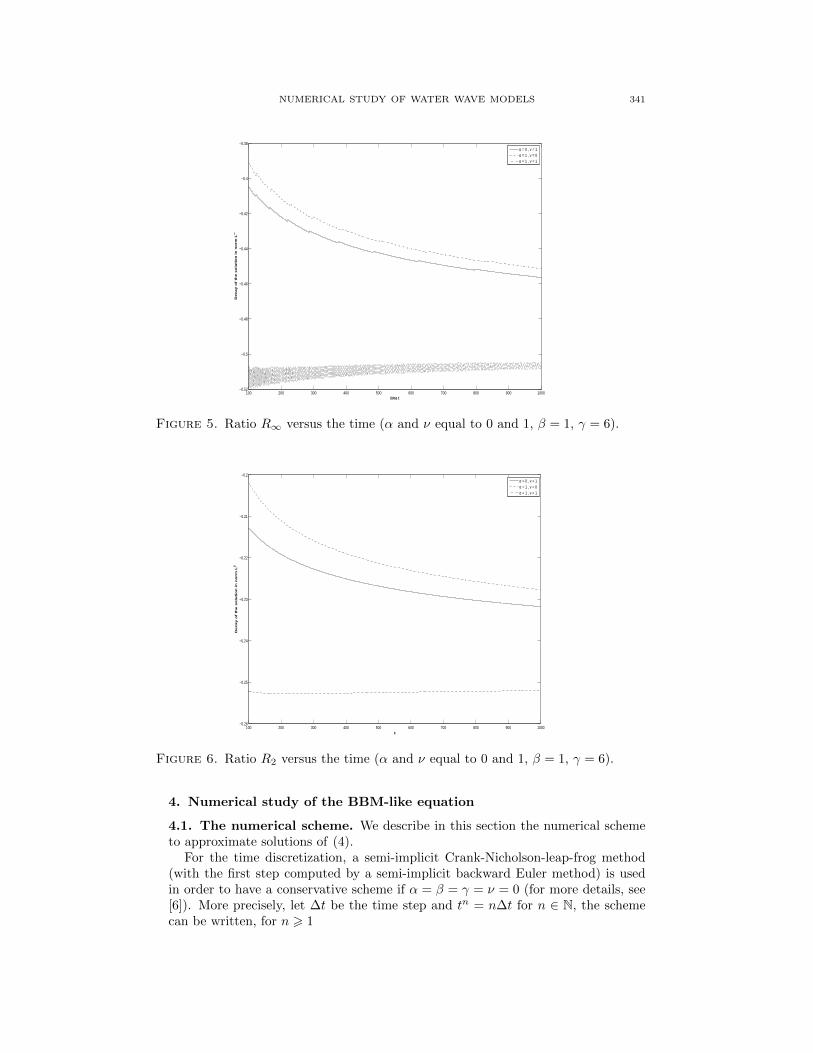
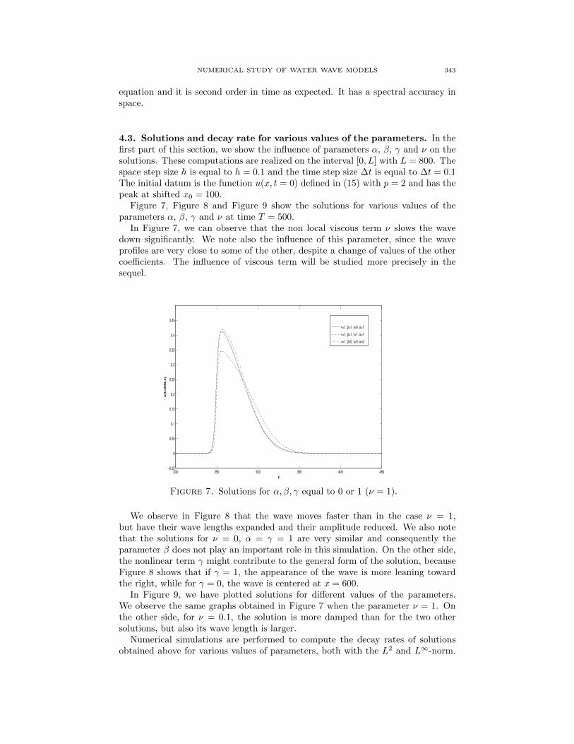
We now investigate numerically the decay rate of the solutions when the localdispersion term uxxx is present. For that we fix firstly β to 1 and γ to 6 and wevary the coefficients α and ν equal to 0 and 1. Finally we present the functions R∞and R2 versus the time t in the Figure 5 and Figure 6.

As for Table 2, we computed the decay rate a of the solutions for these coefficientsand these results are given in Table 3, and shows a decay rate near from − 1

2 for

the L∞-norm and − 14 for the L2-norm.

Table 3. Decay rate of the solution u(t, .) versus the time (νand α equal to 0 and 1, β = 1, γ = 6).

Norm (α, ν) = (0, 1) (α, ν) = (1, 0) (α, ν) = (1, 1)L∞ −0.44 −0.51 −0.43L2 −0.23 −0.25 −0.22

To conclude this section, we can say that the results obtained by the Gearoperator are analogous to those produced in [7]. Therefore the numerical methodusing the Gear operator turns out to be good technique to compute solutions ofthe equation (1).


100 200 300 400 500 600 700 800 900 1000−0.52

−0.5

−0.48

−0.46

−0.44

−0.42

−0.4

−0.38

time t

Decay o

f th

e s

olu

tio

n in

no

rm L

∞

α = 0 , ν = 1α = 1 , ν = 0α = 1 , ν = 1

Figure 5. Ratio R∞ versus the time (α and ν equal to 0 and 1, β = 1, γ = 6).

100 200 300 400 500 600 700 800 900 1000−0.26

−0.25

−0.24

−0.23

−0.22

−0.21

−0.2

x

De

ca

y o

f th

e s

olu

tio

n i

n n

orm

L2

α = 0 , ν = 1α = 1 , ν = 0α = 1 , ν = 1

Figure 6. Ratio R2 versus the time (α and ν equal to 0 and 1, β = 1, γ = 6).

4. Numerical study of the BBM-like equation

4.1. The numerical scheme. We describe in this section the numerical schemeto approximate solutions of (4).

For the time discretization, a semi-implicit Crank-Nicholson-leap-frog method(with the first step computed by a semi-implicit backward Euler method) is usedin order to have a conservative scheme if α = β = γ = ν = 0 (for more details, see[6]). More precisely, let ∆t be the time step and tn = n∆t for n ∈ N, the schemecan be written, for n > 1


(1− β∆)un+1 − un−1

2∆t+√ν(G

12u)n− α

2

(un+1xx + un−1

xx

)+

1

2

(un+1x + un−1

x

)+ γ

1

2(un)2

x = 0,

(13)

where un represents the numerical approximation of u(tn, .), and u0 is the initial

data u0. The viscous term(G

12u)n

(see Section 2) at time tn is approximated by(G

12u)n

=1

2G

12

(un+1 + un−1

)=

1

2

√3

2∆t

n+1∑j=0

gn+1−juj +

n−1∑j=0

gn−1−juj

.

For the space discretization, a Fourier discretization is implemented, so Fast FourierTransforms can be used. Therefore, the periodic boundary condition on an interval[0, L] with large L is used.

The fully discretized problem can be written, denoting by u(ξ) the Fourier trans-form of u at the frequency ξ, for n ≥ 1

(1 + βξ2)(un+1 − un−1

)+

√3ν∆t

2

n+1∑j=0

gn+1−j uj +

n−1∑j=0

gn−1−j uj

+∆t

(αξ2 + iξ

) (un+1 + un−1

)+ iγ∆t ξ ˆ(un)2 = 0

(14)

at time tn = n∆t, and for ξ =2π

Lj, −N

2≤ j ≤ N

2and N is the number of modes

under consideration.

4.2. Validation of the scheme. In order to validate the numerical method usedin the sequel, we will follow the ideas of M. Chen [6]. This technique consistsin neglecting the viscous and viscous diffusion terms in equation (4), and computenumerically the solution of this equation with a known exact solitary-wave solution.With α = ν = 0, β = γ = 1, equation (4) reads

ut + ux − utxx + uux = 0.

Let u(x, t) = ϕ(x− pt), ϕ satisfies

(p− 1)ϕ′ − pϕ′′′ − ϕϕ′ = 0.

Using Lemma 1 in [5], namely αη′ − βη′′′ − ηη′ = 0 admits a solution

η = 3α sech2(

12

√αβx)

, one finds explicit solutions

(15) u(x, t) = ϕ(x− pt) = 3 (p− 1) sech2

(1

2

√p− 1

p(x− pt)

).

The one with p = 2 is used for our test.For an interval of length L = 400 with N = 800 modes, a time step ∆t = 0.01,

the computed solution has ‖u(T, .)‖L∞ equal to 3.00005 at time T = 50 while theexplicit solution has ‖uex(T, .)‖L∞ equal to 3. The maximum difference between thecomputed solution u(T, .) and uex(T, .) at T = 50, ‖uex(T, .) − u(T, .)‖L∞ is equalto 3.05×10−4. By halving the size of ∆t = 0.005, ‖uex(T, .)−u(T, .)‖L∞ decreasedto 7.6 × 10−5. Therefore, the numerical scheme is validated for non-dissipative


equation and it is second order in time as expected. It has a spectral accuracy inspace.

4.3. Solutions and decay rate for various values of the parameters. In thefirst part of this section, we show the influence of parameters α, β, γ and ν on thesolutions. These computations are realized on the interval [0, L] with L = 800. Thespace step size h is equal to h = 0.1 and the time step size ∆t is equal to ∆t = 0.1The initial datum is the function u(x, t = 0) defined in (15) with p = 2 and has thepeak at shifted x0 = 100.

Figure 7, Figure 8 and Figure 9 show the solutions for various values of theparameters α, β, γ and ν at time T = 500.

In Figure 7, we can observe that the non local viscous term ν slows the wavedown significantly. We note also the influence of this parameter, since the waveprofiles are very close to some of the other, despite a change of values of the othercoefficients. The influence of viscous term will be studied more precisely in thesequel.

200 250 300 350 400 450−0.05

0

0.05

0.1

0.15

0.2

0.25

0.3

0.35

0.4

0.45

x

u(t=500,x)

ν=1, β=1, γ=0, α=1

ν=1, β=1, γ=1, α=1

ν=1, β=0, γ=0, α=0

Figure 7. Solutions for α, β, γ equal to 0 or 1 (ν = 1).

We observe in Figure 8 that the wave moves faster than in the case ν = 1,but have their wave lengths expanded and their amplitude reduced. We also notethat the solutions for ν = 0, α = γ = 1 are very similar and consequently theparameter β does not play an important role in this simulation. On the other side,the nonlinear term γ might contribute to the general form of the solution, becauseFigure 8 shows that if γ = 1, the appearance of the wave is more leaning towardthe right, while for γ = 0, the wave is centered at x = 600.

In Figure 9, we have plotted solutions for different values of the parameters.We observe the same graphs obtained in Figure 7 when the parameter ν = 1. Onthe other side, for ν = 0.1, the solution is more damped than for the two othersolutions, but also its wave length is larger.

Numerical simulations are performed to compute the decay rates of solutionsobtained above for various values of parameters, both with the L2 and L∞-norm.


400 450 500 550 600 650 700 750 800−0.05

0

0.05

0.1

0.15

0.2

0.25

x

u(t=500,x)

ν=0, β=1, γ=1, α=1

ν=0, β=1, γ=0, α=1

ν=0, β=0, γ=1, α=1

Figure 8. Solutions for α, β, γ equal to 0 or 1 (ν = 0).

250 300 350 400 450

0

0.1

0.2

0.3

0.4

0.5

x

u(t=500,x)

ν=1, β=0.1, γ=1, α=1

ν=0.1, β=1, γ=0, α=1

ν=1, β=0, γ=0.1, α=0.1

Figure 9. Solutions for α, β, γ and ν equal to 0, 0.1 or 1.

For this computation, the domain of computation, the space step and time ofdiscretization and the initial datum remain unchanged.

The functions R2 and R∞ versus the time t are plotted in Figure 10 and 11for ν = 1, Figure 12 and 13 for various values of parameters. The values of thedecay rate are presented in Table 4. Looking more closely at these results on thedecay rates, there is a certain similarity with the results for equation (1). That isto say, when the non local viscosity occurs, the decay rate are around −0.24 for theL2-norm as in equation (1) and are around −0.48 for the L∞-norm. We can saythat both solutions of KdV and BBM equations with the non local viscosity termhave nearly the same decay rate.


Table 4. Decay rate of the solution u(t, .) versus the time for variousvalues of the parameters.

Viscosity Dispersive Non linear Diffusion L2 L∞

ν term β term γ term α decay rate decay rate1 1 0 1 −0.22 −0.451 1 1 1 −0.20 −0.401 0 0 0 −0.24 −0.480 1 1 1 −0.25 −0.520 1 0 1 −0.25 −0.490 0 1 1 −0.25 −0.501 0.1 1 1 −0.20 −0.39

0.1 1 0 1 −0.28 −0.541 0 0.1 0.1 −0.23 −0.46

50 100 150 200 250 300 350 400 450 500−0.26

−0.25

−0.24

−0.23

−0.22

−0.21

−0.2

−0.19

−0.18

−0.17

time t

Decay o

f th

e s

olu

tio

n in

no

rm

L2

ν=1, β=1, γ=0, α=1

ν=1, β=1, γ=1, α=1

ν=1, β=0, γ=0, α=0

Figure 10. Ratio R2 versus the time t for α, β, γ equal to 0 or 1 (ν = 1).

4.4. Influence of the magnitude of the viscosity. In this subsection, numer-ical experiments are performed to study the influence of the viscosity on the decayrate. In these computations, the data are: L = 2000, h = 0.2, ∆t = 0.2, T = 1000,α = 0 and β = γ = 1. In these experiments, the initial datum is the function (15)with p = 2, and shift around the point x0 = L/2.

The solutions at T = 1000 for equations with various ν between 0.1 and 20are plotted in Figure 14. As expected, we observe that the viscosity increases thedamping of the wave. In addition, the velocity of the wave also decreases with theviscosity.

The ratio R2 and R∞ versus the time t are plotted in Figure 15 and 16 fordifferent values of ν. The values of decay rate are shown in Table 5. We noticeimmediately in Table 5 the influence of viscosity, because the more the values ofν increases, the more the value of decay rate in L2 and L∞-norm decreases. Thisresults are consistent with comments made on the Figure 14.


50 100 150 200 250 300 350 400 450 500−0.5

−0.48

−0.46

−0.44

−0.42

−0.4

−0.38

−0.36

−0.34

−0.32

time t

De

ca

y o

f th

e s

olu

tio

n i

n n

orm

L∞

ν=1, β=1, γ=0, α=1

ν=1, β=1, γ=1, α=1

ν=1, β=0, γ=0, α=0

Figure 11. Ratio R∞ versus the time t for α, β, γ equal to 0 or 1 (ν = 1).

50 100 150 200 250 300 350 400 450 500−0.32

−0.3

−0.28

−0.26

−0.24

−0.22

−0.2

−0.18

time t

Decay o

f th

e s

olu

tio

n in

no

rm

L2

ν=1, β=0.1, γ=1, α=1

ν=0.1, β=1, γ=0, α=1

ν=1, β=0, γ=0.1, α=0.1

Figure 12. Ratio R2 versus the time t for α, β, γ and ν equal to 0, 0.1 or 1.

5. Conclusion

In this paper, we propose a discretization of the non local viscosity using a Gα-scheme. The technique permits us to study the influence of the viscosity on thedecay rate for the viscous KdV-like equation and compare these results to thoseobtained in [7]. Moreover, a study of the influence of the viscosity on the viscousBBM-like equation is presented, study that can not be allowed using techniquesdeveloped in [7].


50 100 150 200 250 300 350 400 450 500−0.65

−0.6

−0.55

−0.5

−0.45

−0.4

−0.35

−0.3

time t

Decay o

f th

e s

olu

tio

n in

no

rm

L∞

ν=1, β=0.1, γ=1, α=1

ν=0.1, β=1, γ=0, α=1

ν=1, β=0, γ=0.1, α=0.1

Figure 13. Ratio R∞ versus the time t for α, β, γ and ν equal to 0, 0.1 or 1.

Table 5. Decay rate of the solution u(t, .) versus the time for variousvalues of ν (β = γ = 1 and α = 0).

Viscosity L2 L∞

ν decay rate decay rate0.1 −0.26 −0.470.5 −0.23 −0.431 −0.21 −0.412 −0.20 −0.395 −0.18 −0.3510 −0.17 −0.3220 −0.15 −0.30

References

[1] C. J. Amick, J. L. Bona and M. E. Schonbek, Decay of solutions of some nonlinear waveequations, J. Differential Equations, 81 (1989), pp. 1-49.

[2] J. L. Bona, M. Chen and J.-C. Saut, Boussinesq equations and other systems for small-

amplitude long waves in nonlinear dispersive media, I, Derivation and the linear theory, J.Nonlinear Sci., 12, 2002, pp. 283-318.

[3] J. L. Bona, F. Demengel and K. Promislow, Fourier splitting and dissipation of nonlinear

dispersive waves, Proc. Roy. Soc. Edinburgh Sect. A 129 (1999), No. 3, pp. 477-502.[4] J. L. Bona, K. Promislow and C. E. Wayne, Higher-order asymptotics of decaying solutions

of some nonlinear, dispersive, dissipative wave equations, Nonlinearity 8 (1995), No. 6, pp.1179-1206.

[5] M. Chen, Exact Traveling-wave solutions to bi-directional wave equations, InternationalJournal of Theoretical Physics, vol. 37, Number 5, 1998, pp. 1547-1567.

[6] M. Chen, Numerical investigation of a two-dimensional Boussinesq system, Discrete Contin.

Dyn. Syst., Vol 28, 2009, No. 4, pp. 1169-1190.[7] M. Chen, S. Dumont, L. Dupaigne and O. Goubet, Decay of solutions to a water wave model

with a nonlocal viscous dispersive term, Discrete Contin. Dyn. Syst., 27, 2010, No. 4, pp.

1473-1492.


950 1000 1050 1100 1150 1200 1250 1300 1350 1400 1450

0

0.1

0.2

0.3

0.4

0.5

0.6

0.7

0.8

0.9

1

x

u(t=1000,x)

BBM soliton

ν = 0.1

ν = 0.5

ν = 1

ν = 2

ν = 5

ν = 10

ν = 20

Figure 14. Solutions for the viscosity ν ranging from 0.1 to 20.

100 200 300 400 500 600 700 800 900 1000−0.3

−0.28

−0.26

−0.24

−0.22

−0.2

−0.18

−0.16

−0.14

−0.12

−0.1

time t

De

ca

y o

f th

e s

olu

tio

n i

n n

orm

L2

ν = 0.1

ν = 0.5

ν = 1

ν = 2

ν = 5

ν = 10

ν = 20

Figure 15. Ratio R2 versus the time t for ν ranging from 0.1 to 20.

[8] M. Chen and O. Goubet, Long-Time Asymptotic Behavior of 2D Dissipative BoussinesqSystem, Discrete Contin. Dyn. Syst., Vol. 17, Number 3, 2007, pp. 509-528.

[9] A.-C. Galucio , J.-F. Deu, S. Mengue and F. Dubois, An adaptation of the Gear scheme forfractionnal derivatives, Comput. Methods Appl. Mech. Engrg., 195(2006), pp. 6073-6085.

[10] F. Dubois, A.-C. Galucio and N. Point, Introduction a la derivation fractionnaire - Theorie

et Applications, http://www.math.u-psud.fr/fdubois/travaux/evolution/ananelly-07/

techinge08/techinge-01nov08.pdf.

[11] D. Dutykh, Visco-potential free-surface flows and long wave modeling, European Journal of

Mechanics B/Fluids, 28(3), 2009, pp. 430-443.


100 200 300 400 500 600 700 800 900 1000−0.5

−0.45

−0.4

−0.35

−0.3

−0.25

−0.2

−0.15

time t

De

ca

y o

f th

e s

olu

tio

n i

n n

orm

L∞

ν = 0.1

ν = 0.5

ν = 1

ν = 2

ν = 5

ν = 10

ν = 20

Figure 16. Ratio R∞ versus the time t for ν ranging from 0.1 to 20.

[12] D. Dutykh and F. Dias, Viscous potential free-surface flows in a fluid layer of finite depth,C. R. Math. Acad. Sci. Paris, 345, 2007, pp. 113-118.

[13] O. Goubet and G. Warnault, Decay of solutions to a linear viscous asymptotic model for

water waves, Chin. Ann. Math. Ser. B, Vol. 31, No. 6, 2010, pp. 841-854.[14] T. Kakutani and K. Matsuuchi, Effect of viscosity of long gravity waves, J. Phys. Soc. Japan,

39, 1975, pp. 237-246.[15] P. Liu and A. Orfila, Viscous effects on transcient long-wave propagation, J. Fluid Mech.,

520, 2004, pp. 83-92.

[16] K. Pen-Yu, J. M. Sanz-Serna, Convergence of methods for the numerical solution of theKorteweg-de-Vries equation, IMA Journal of Numerical Analysis, 1 (1981), 215-221.

LAMFA CNRS UMR 7352, Universite de Picardie Jules Verne, 33, rue Saint-Leu, 80039

Amiens, France.

E-mail : [email protected]

URL: http://lamfa.u-picardie.fr/dumont/

LMAC EA 2222, Universite de Technologie de Compiegne, Centre de Recherches de Royallieu,60205 Compiegne, France.

E-mail : [email protected]

URL: http://lamfa.u-picardie.fr/duval

Documents

NUMERICAL INVESTIGATION OF THE DECAY RATE OF … · t s ds+ uux= uxx: in the BBM form. In order to realize this numerical study, a numerical scheme based of the ... (s) t s dsstands