Numerical IntegrationNumerical Integration

• Trapezoidal Rule

• Simpson’s Rule

– 1/3 Rule

Basic Numerical Integration

– 1/3 Rule

– 3/8 Rule

• Midpoint

• Gaussian Quadrature

Basic Numerical IntegrationBasic Numerical Integration

We want to find integration of functions of various forms of the equation known as the Newton Cotes integration formulas.Newton Cotes integration formulas.

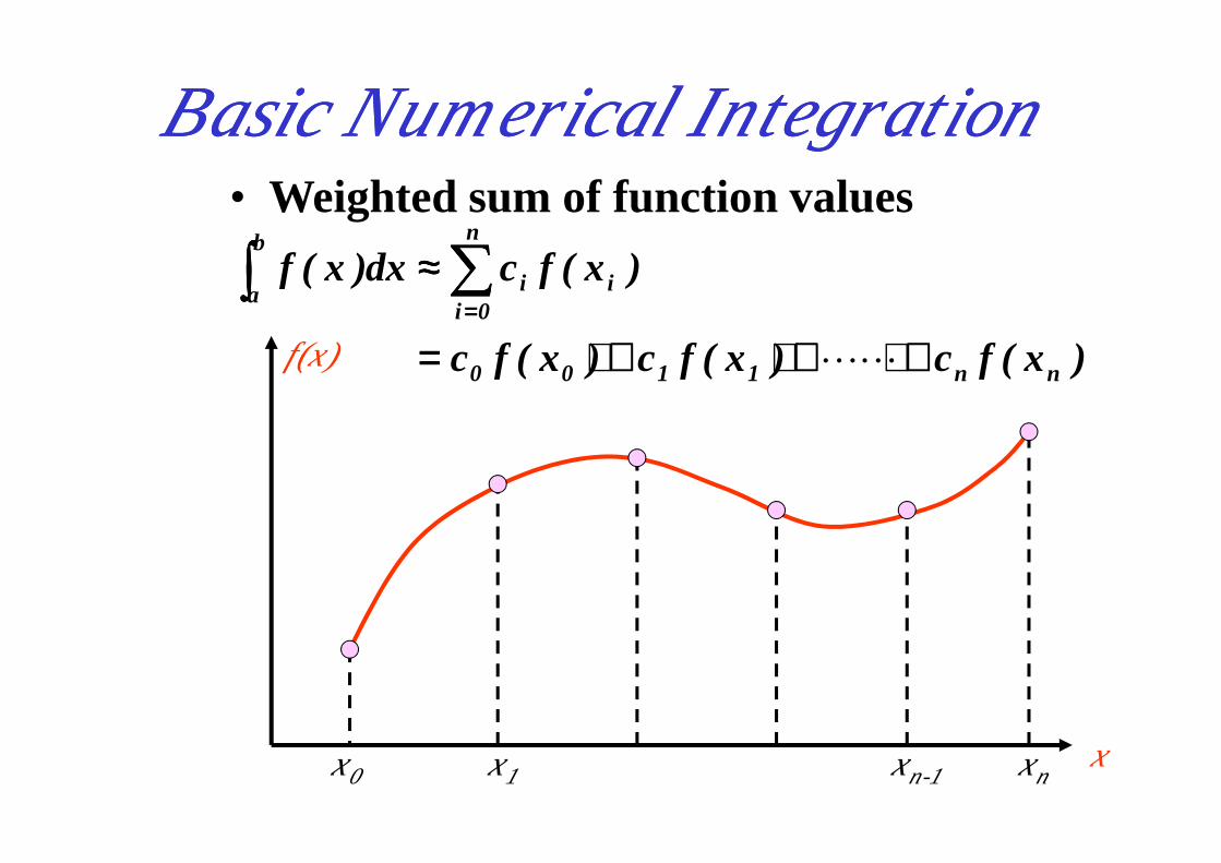
Basic Numerical IntegrationBasic Numerical Integration• Weighted sum of function values

)x(fc)x(fc)x(fc

)x(fcdx)x(f

nn1100

i

n

0ii

b

a

++++++++++++====

≈≈≈≈∑∑∑∑∫∫∫∫====

LLf(x)

x0 x1 xnxn-1x

12

Numerical IntegrationNumerical IntegrationIdea is to do integral in small parts, like the way you first learned integration - a summation

Numerical methods just try to make it faster and more accurate

0

2

4

6

8

10

3 5 7 9 11 13 15

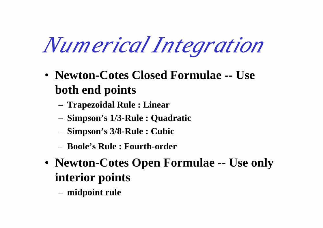
Numerical IntegrationNumerical Integration• Newton-Cotes Closed Formulae -- Use

both end points– Trapezoidal Rule : Linear– Simpson’s 1/3-Rule : Quadratic– Simpson’s 1/3-Rule : Quadratic– Simpson’s 3/8-Rule : Cubic

– Boole’s Rule : Fourth-order

• Newton-Cotes Open Formulae -- Use only interior points– midpoint rule

Trapezoid RuleTrapezoid Rule• Straight-line approximation

[[[[ ]]]])x(f)x(f2h

)x(fc)x(fc)x(fcdx)x(f

10

1100i

1

0ii

b

a

++++====

++++====≈≈≈≈∑∑∑∑∫∫∫∫====

2

x0 x1x

f(x)

L(x)

Trapezoid RuleTrapezoid Rule

• Lagrange interpolation

010 1

0 1 1 0

( ) ( ) ( )x xx x

L x f x f xx x x x

−−= +− −0 1 1 0

0 1

dx a x , b x , , d ;

h

0( ) (1 ) ( ) ( ) ( )

1

x x x x

x alet h b a

b a

x aL f a f b

x b

ξ ξ

ξξ ξ ξ

ξ

− −−= = = = = −−

= ⇒ = ⇒ = − + = ⇒ =

Trapezoid RuleTrapezoid Rule

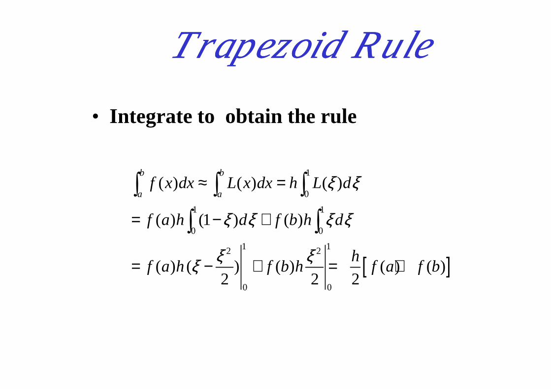
• Integrate to obtain the rule

1

0( ) ( ) ( )

b b

a af x dx L x dx h L dξ ξ≈ =∫ ∫ ∫

[ ]

0

1 1

0 0

1 12 2

0 0

( ) (1 ) ( )

( ) ( ) ( ) ( ) ( )2 2 2

a a

f a h d f b h d

hf a h f b h f a f b

ξ ξ ξ ξ

ξ ξξ

= − +

= − + = +

∫ ∫ ∫

∫ ∫

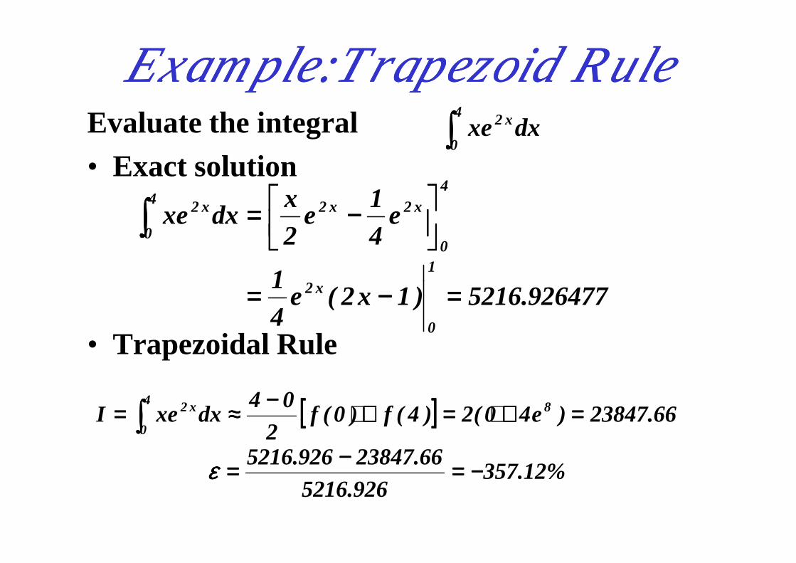
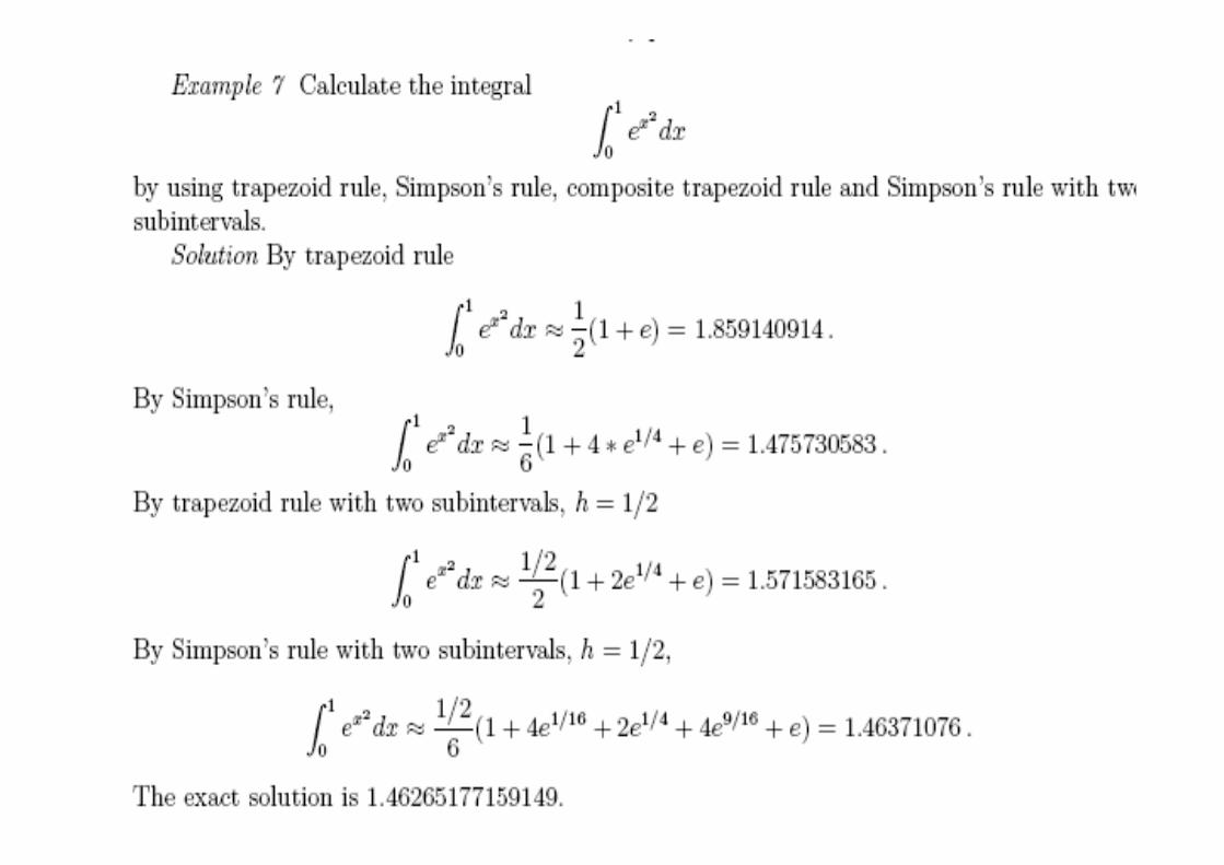
Example:Trapezoid RuleExample:Trapezoid RuleEvaluate the integral• Exact solution

926477.5216)1x2(e1

e41

e2x

dxxe

1x2

4

0

x2x24

0

x2

====−−−−====

−−−−====∫∫∫∫

dxxe4

0

x2∫∫∫∫

• Trapezoidal Rule

926477.5216)1x2(e41

0

x2 ====−−−−====

[[[[ ]]]]

%12.357926.5216

66.23847926.5216

66.23847)e40(2)4(f)0(f2

04dxxeI 84

0

x2

−−−−====−−−−====

====++++====++++−−−−≈≈≈≈==== ∫∫∫∫

εεεε

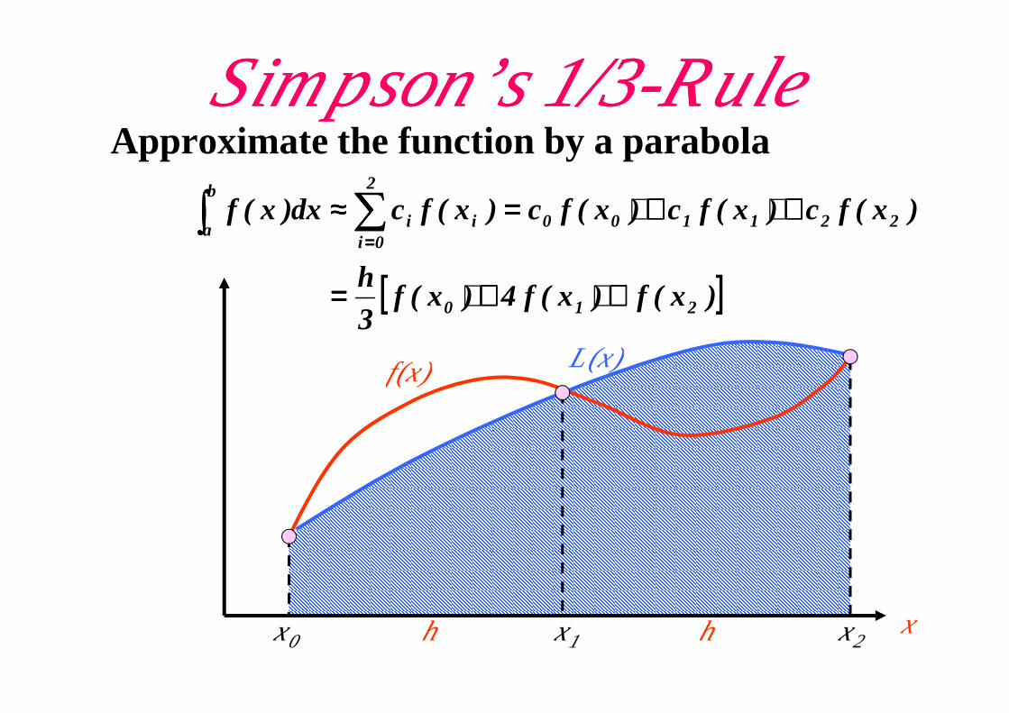
Simpson’s Simpson’s 11//33--RuleRuleApproximate the function by a parabola

[[[[ ]]]])x(f)x(f4)x(f3h

)x(fc)x(fc)x(fc)x(fcdx)x(f

210

221100i

2

0ii

b

a

++++++++====

++++++++====≈≈≈≈∑∑∑∑∫∫∫∫====

f(x) L(x)

x0 x1x

f(x)

x2h h

L(x)

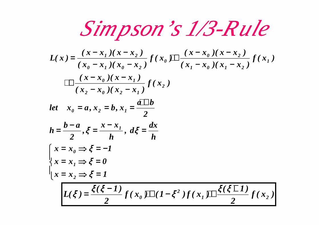
Simpson’s Simpson’s 11//33--RuleRule

++++============

−−−−−−−−−−−−−−−−

++++

−−−−−−−−−−−−−−−−++++

−−−−−−−−−−−−−−−−====

2ba

x ,bx ,ax let

)x(f)xx)(xx(

)xx)(xx(

)x(f)xx)(xx(

)xx)(xx( )x(f

)xx)(xx(

)xx)(xx()x(L

120

21202

10

12101

200

2010

21

====⇒⇒⇒⇒========⇒⇒⇒⇒====

−−−−====⇒⇒⇒⇒====

====−−−−====−−−−====

1 xx

0 xx

1 xxh

dxd ,

h

xx ,

2ab

h

2

2

1

0

1

120

ξξξξξξξξξξξξ

ξξξξξξξξ

)x(f2

)1()x(f)1()x(f

2)1(

)(L 212

0

++++++++−−−−++++−−−−==== ξξξξξξξξξξξξξξξξξξξξξξξξ

Simpson’s Simpson’s 11//33--RuleRule

11

1

12

1

0

21

1

10

1

1

b

a

)dξ1ξ(ξ2h

)f(x)dξξ1()hf(x

)dξ1ξ(ξ2h

)f(xdξ)(Lhf(x)dx

−−−−

−−−−−−−−

++++++++−−−−++++

−−−−====≈≈≈≈

∫∫∫∫∫∫∫∫

∫∫∫∫∫∫∫∫∫∫∫∫ ξξξξ

Integrate the Lagrange interpolation

1

1

23

2

1

1

3

1

1

1

23

0

)2ξ

3ξ

(2h

)f(x

)3ξ

(ξ)hf(x)2ξ

3ξ

(2h

)f(x

−−−−

−−−−−−−−

++++++++

−−−−++++−−−−====

[[[[ ]]]])f(x)4f(x)f(x3h

f(x)dx 210

b

a++++++++====∫∫∫∫

Simpson’s Simpson’s 33//88--RuleRuleApproximate by a cubic polynomial

[[[[ ]]]])x(f)x(f3)x(f3)x(f8h3

)f(xc)f(xc)f(xc)f(xc)x(fcdx)x(f

3210

33221100i

3

0ii

b

a

++++++++++++====

++++++++++++====≈≈≈≈∑∑∑∑∫∫∫∫====

f(x)L(x)

x0 x1x

f(x)

x2h h

L(x)

x3h

Simpson’s Simpson’s 33//88--RuleRule

)x(f)xx)(xx)(xx(

)xx)(xx)(xx(

)x(f)xx)(xx)(xx(

)xx)(xx)(xx(

)x(f)xx)(xx)(xx(

)xx)(xx)(xx()x(L

2321202

310

1312101

320

0302010

321

−−−−−−−−−−−−−−−−−−−−−−−−

++++

−−−−−−−−−−−−−−−−−−−−−−−−

++++

−−−−−−−−−−−−−−−−−−−−−−−−

====

)x(f)xx)(xx)(xx(

)xx)(xx)(xx(

)xx)(xx)(xx(

3231303

210

321202

−−−−−−−−−−−−−−−−−−−−−−−−

++++

−−−−−−−−−−−−

[[[[ ]]]])x(f)x(f3)x(f3)x(f8h3

3a-b

h ; L(x)dxf(x)dx

3210

b

a

b

a

++++++++++++====

====≈≈≈≈ ∫∫∫∫∫∫∫∫

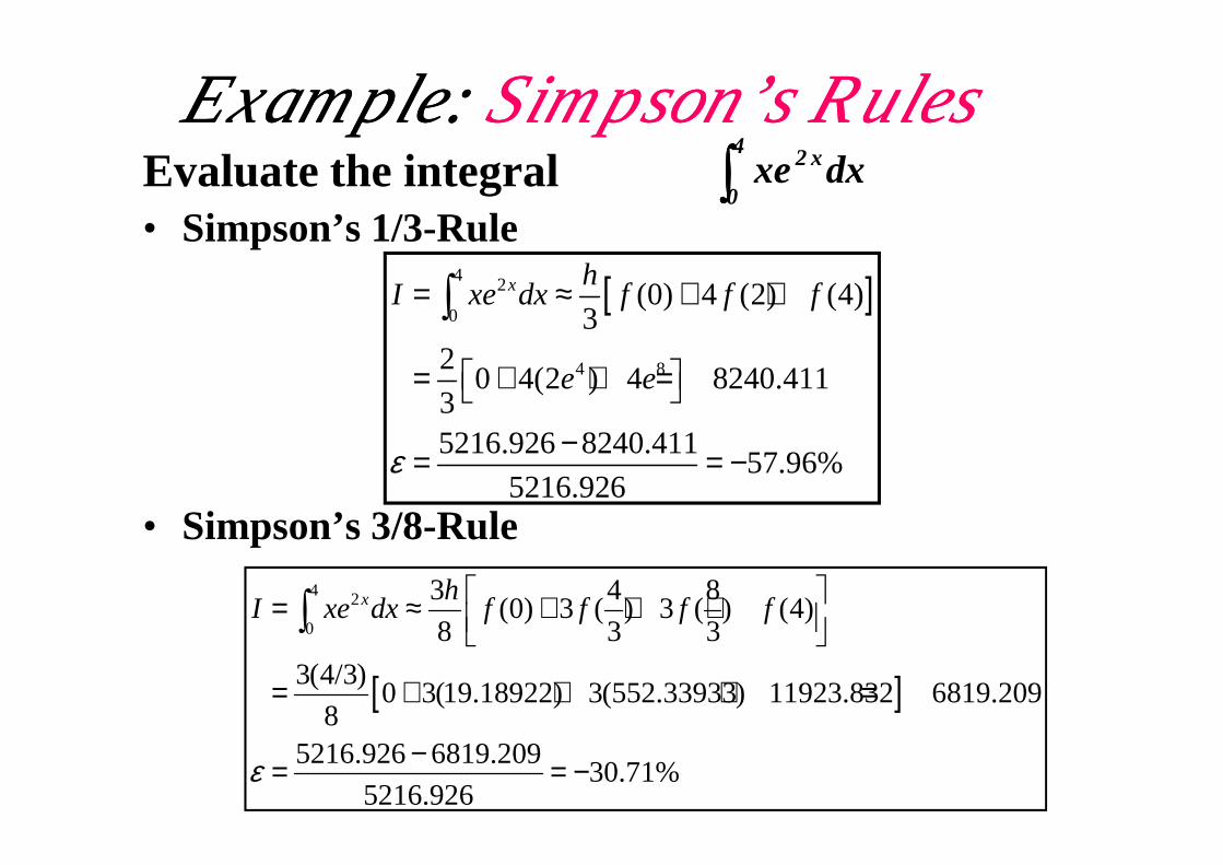
Example: Example: Simpson’s RulesSimpson’s RulesEvaluate the integral• Simpson’s 1/3-Rule

dxxe4

0

x2∫∫∫∫

[ ]4 2

0

4 8

(0) 4 (2) (4)3

20 4(2 ) 4 8240.411

35216.926 8240.411

x hI xe dx f f f

e e

= ≈ + +

= + + =

−

∫

• Simpson’s 3/8-Rule

5216.926 8240.41157.96%

5216.926ε −= = −

[ ]

4 2

0

3 4 8(0) 3 ( ) 3 ( ) (4)

8 3 3

3(4/3)0 3(19.18922) 3(552.33933)11923.832 6819.209

85216.926 6819.209

30.71%5216.926

x hI xe dx f f f f

ε

= ≈ + + +

= + + + =

−= = −

∫

Midpoint RuleMidpoint RuleNewton-Cotes Open Formula

)(f24

)ab()

2ba

(f)ab(

)x(f)ab(dx)x(f3

m

b

a

ηηηη′′′′′′′′−−−−++++++++−−−−====

−−−−≈≈≈≈∫∫∫∫

f(x)

a b x

f(x)

xm

Better Numerical IntegrationBetter Numerical Integration

• Composite integration – Composite Trapezoidal Rule

– Composite Simpson’s Rule

• Richardson Extrapolation• Richardson Extrapolation• Romberg integration

Apply trapezoid rule to multiple segments over Apply trapezoid rule to multiple segments over integration limitsintegration limits

2

3

4

5

6

7

Two segments

2

3

4

5

6

7

Three segments

0

1

3 5 7 9 11 13 15

0

1

2

3

4

5

6

7

3 5 7 9 11 13 15

Four segments

0

1

2

3

4

5

6

7

3 5 7 9 11 13 15

Many segments

0

1

3 5 7 9 11 13 15

Composite Trapezoid RuleComposite Trapezoid Rule

[[[[ ]]]] [[[[ ]]]] [[[[ ]]]]

[[[[ ]]]])x(f)x(f2)2f(x)f(x2)f(x2h

)f(x)f(x2h

)f(x)f(x2h

)f(x)f(x2h

f(x)dxf(x)dxf(x)dxf(x)dx

n1ni10

n1n2110

x

x

x

x

x

x

b

a

n

1n

2

1

1

0

++++++++++++++++++++++++====

++++++++++++++++++++++++====

++++++++++++====

−−−−

−−−−

∫∫∫∫∫∫∫∫∫∫∫∫∫∫∫∫−−−−

LL

L

LL

f(x)

x0 x1x

f(x)

x2h h x3h h x4

nab

h−−−−====

Composite Trapezoid RuleComposite Trapezoid RuleEvaluate the integral dxxeI

4

0

x2∫∫∫∫====

[[[[ ]]]]

[[[[ ]]]]

[[[[ )2(f2)1(f2)0(f2h

I1h,4n

%75.132 23.12142)4(f)2(f2)0(f2h

I2h,2n

%12.357 66.23847)4(f)0(f2h

I4h,1n

++++++++====⇒⇒⇒⇒========

−−−−========++++++++====⇒⇒⇒⇒========

−−−−========++++====⇒⇒⇒⇒========

εεεε

εεεε

[[[[]]]]

[[[[

]]]][[[[

]]]]%66.2 95.5355

)4(f)75.3(f2)5.3(f2

)5.0(f2)25.0(f2)0(f2h

I25.0h,16n

%50.10 76.5764)4(f)5.3(f2 )3(f2)5.2(f2)2(f2)5.1(f2

)1(f2)5.0(f2)0(f2h

I5.0h,8n

%71.39 79.7288)4(f)3(f2

)2(f2)1(f2)0(f2

I1h,4n

−−−−========++++++++++++

++++++++++++====⇒⇒⇒⇒========

−−−−========++++++++++++++++++++++++

++++++++====⇒⇒⇒⇒========

−−−−========++++++++

++++++++====⇒⇒⇒⇒========

εεεε

εεεε

εεεε

L

Composite TrapezoidComposite TrapezoidExampleExample

∫2 1

dxx f(x)

1.00 0.5000∫ +1 1

1dx

x1.00 0.50001.25 0.44441.50 0.40001.75 0.36362.00 0.3333

Composite Trapezoid Rule with Composite Trapezoid Rule with Unequal SegmentsUnequal Segments

Evaluate the integral• h1 = 2, h2 = 1, h3 = 0.5, h4 = 0.5

dxxeI4

0

x2∫∫∫∫====

[ ] [ ]

)()()()(4

5.3

5.3

3

3

2

2

0+++= ∫∫∫∫

hh

dxxfdxxfdxxfdxxfI

[ ] [ ]

[ ] [ ]

[ ] [ ] [ ][ ] %45.14 58.5971 45.3

2

0.5

5.33e 2

0.532

2

120

2

2

)4()5.3(2

)5.3()3(2

)3()2(2

)2()0(2

87

76644

43

21

−=⇒=++

+++++=

++++

+++=

εee

eeee

ffh

ffh

ffh

ffh

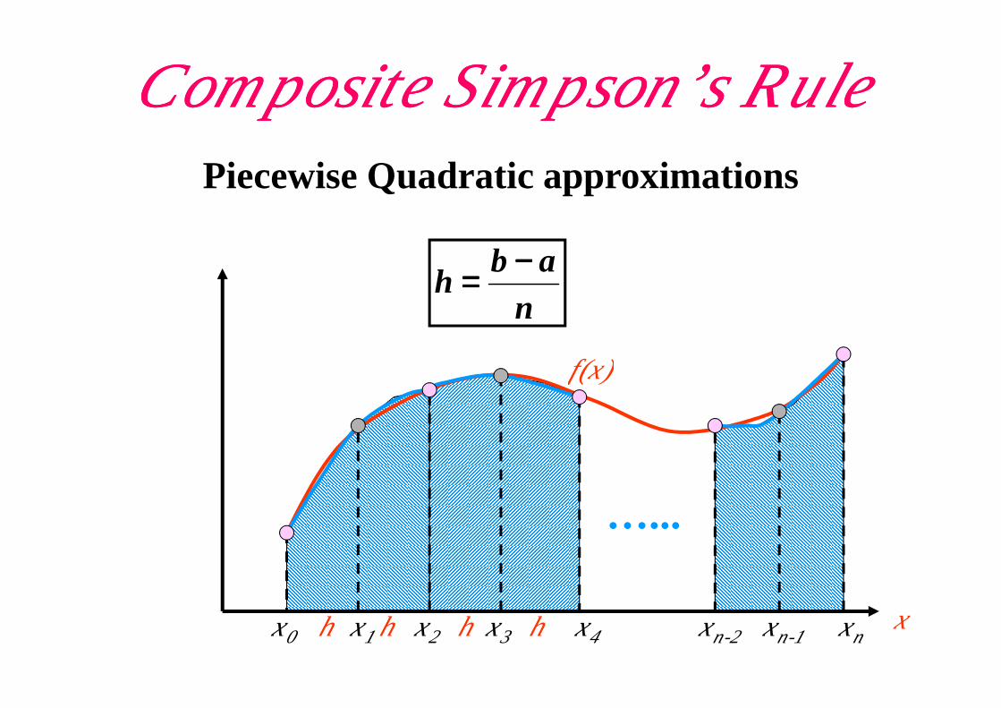
Composite Simpson’s RuleComposite Simpson’s Rule

f(x)

nab

h−−−−====

Piecewise Quadratic approximations

x0 x2x

f(x)

x4h h xn-2h xn

…...

hx3x1 xn-1

[[[[ ]]]] [[[[ ]]]])f(x)f(x4)f(x3h

)f(x)f(x4)f(x3h

f(x)dxf(x)dxf(x)dxf(x)dx

432210

x

x

x

x

x

x

b

a

n

2n

4

2

2

0

++++++++++++++++++++====

++++++++++++==== ∫∫∫∫∫∫∫∫∫∫∫∫∫∫∫∫−−−−

L

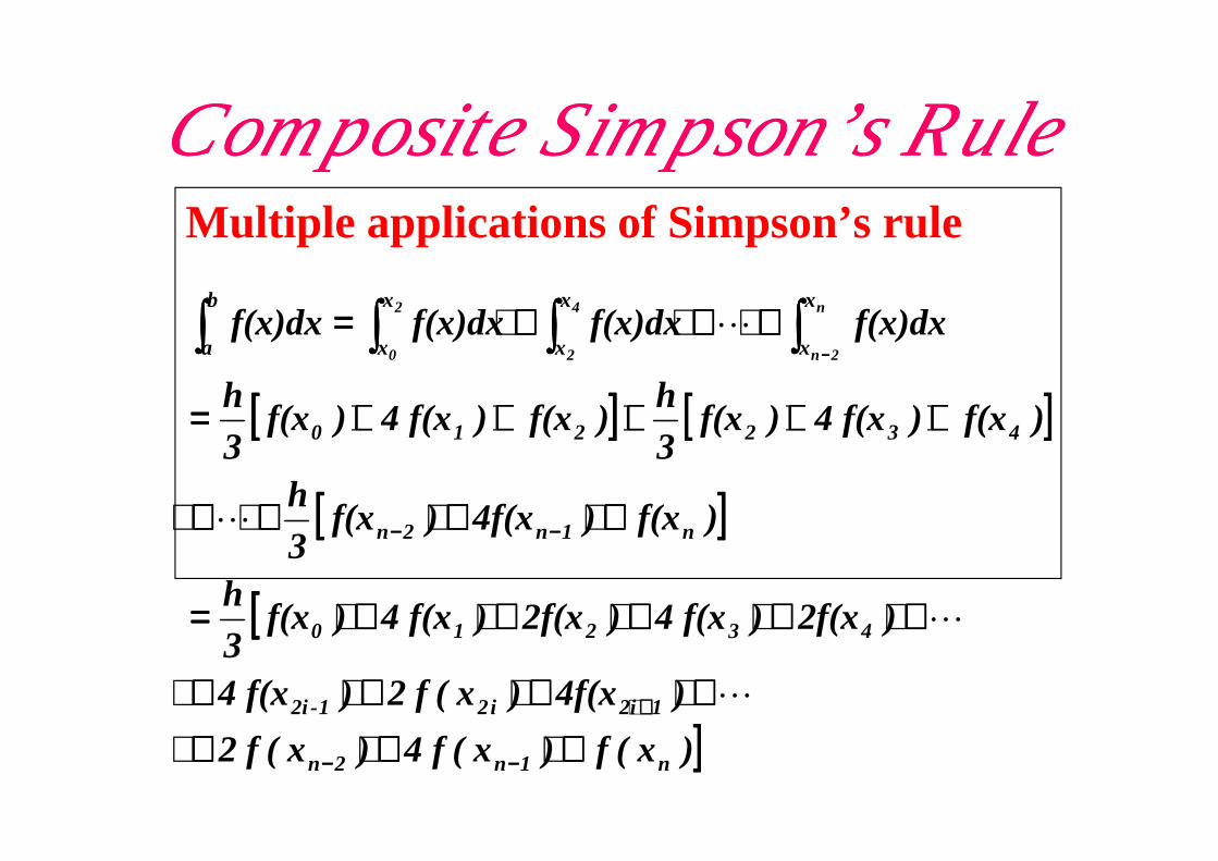
Composite Simpson’s RuleComposite Simpson’s RuleMultiple applications of Simpson’s rule

[[[[ ]]]] [[[[ ]]]]

[[[[ ]]]]

[[[[

]]]])x(f)x(f4)x(f2

)4f(x)x(f2)f(x4

)2f(x)f(x4)2f(x)f(x4)f(x3h

)f(x)4f(x)f(x3h

)f(x)f(x4)f(x3

)f(x)f(x4)f(x3

n1n2n

12ii21-2i

43210

n1n2n

432210

++++++++++++++++++++++++++++

++++++++++++++++++++====

++++++++++++++++

++++++++++++++++++++====

−−−−−−−−

++++

−−−−−−−−

L

L

L

Composite Simpson’s RuleComposite Simpson’s RuleEvaluate the integral• n = 2, h = 2

dxxeI4

0

x2∫∫∫∫====

[[[[ ]]]]

[[[[ ]]]] %96.57 411.8240e4)e2(402

)4(f)2(f4)0(f3h

I

84 −−−−====⇒⇒⇒⇒====++++++++====

++++++++====

εεεε

• n = 4, h = 1

[[[[ ]]]]

[[[[ ]]]]%70.8 975.5670

e4)e3(4)e2(2)e(4031

)4(f)3(f4)2(f2)1(f4)0(f3h

I

8642

−−−−====⇒⇒⇒⇒====

++++++++++++++++====

++++++++++++++++====

εεεε

[[[[ ]]]] %96.57 411.8240e4)e2(403

−−−−====⇒⇒⇒⇒====++++++++==== εεεε

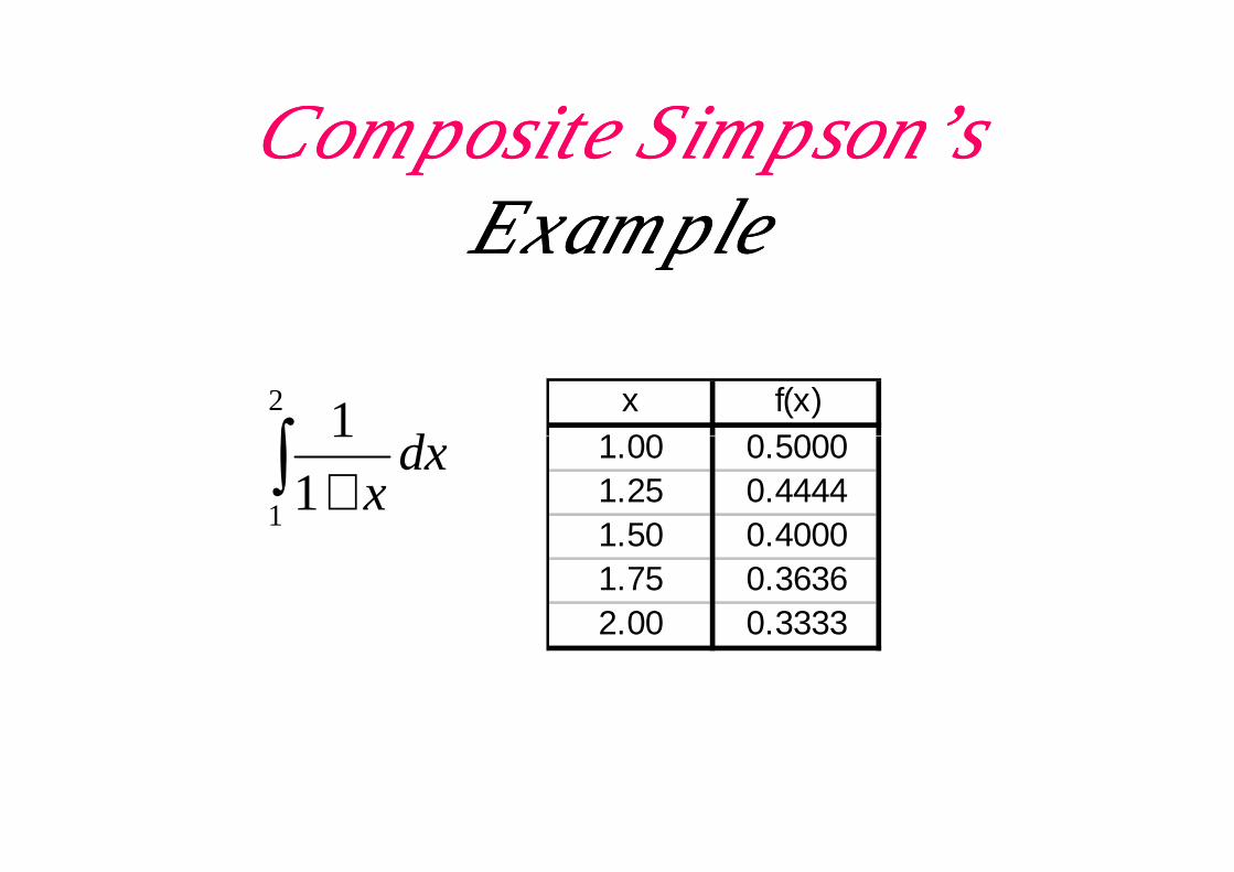
Composite Simpson’sComposite Simpson’sExampleExample

∫2 1

dxx f(x)

1.00 0.5000∫ +1 1

1dx

x1.00 0.50001.25 0.44441.50 0.40001.75 0.36362.00 0.3333

Composite Simpson’s Rule with Composite Simpson’s Rule with Unequal SegmentsUnequal Segments

Evaluate the integral• h1 = 1.5, h2 = 0.5

dxxeI4

0

x2∫∫∫∫====

)()(4

3

3

0+= ∫∫ dxxfdxxfI

[ ]

[ ]

[ ] [ ]%76.3 23.5413

4)5.3(433

5.03)5.1(40

3

5.1

)4(2)5.3(4)3(3

)3(2)5.1(4)0(3

87663

2

1

−=⇒=

+++++=

+++

++=

ε

eeeee

fffh

fffh

Example f(x)= e-x2

[ ]

[ ] 731.0368.0)779.0(215.0

5.0

684.0368.012

11

)()(2)(2

1

10

=++=→=

=+=→=

++= ∑

−

=

Th

Th

xfxfxfh

Tn

ini

lTrapezoida

0

0.25

0.5

0.75

1

exp(-x2)

trapezoidalh=1h=0.5

[ ]

[ ]

[ ]

[ ] 7469.0368.0)570.0(4)779.0(2)939.0(41325.0

25.0

7472.0368.0)779.0(413

5.05.0

)()(2)(4)(3

743.0368.0)570.0(2)779.0(2)939.0(212

25.025.0

731.0368.0)779.0(212

5.05.0

1

..3,1

2

..4,20

=++++=→=

=++=→=

+++=

=++++=→=

=++=→=

∑ ∑−

=

−

=

Sh

Sh

xfxfxfxfh

S

Th

Th

n

i

n

inii

sSimpson'

0 0.25 0.5 0.75 1

The error for NewtonCotes formulas

• The error for Newton Cotes formulas can be given by

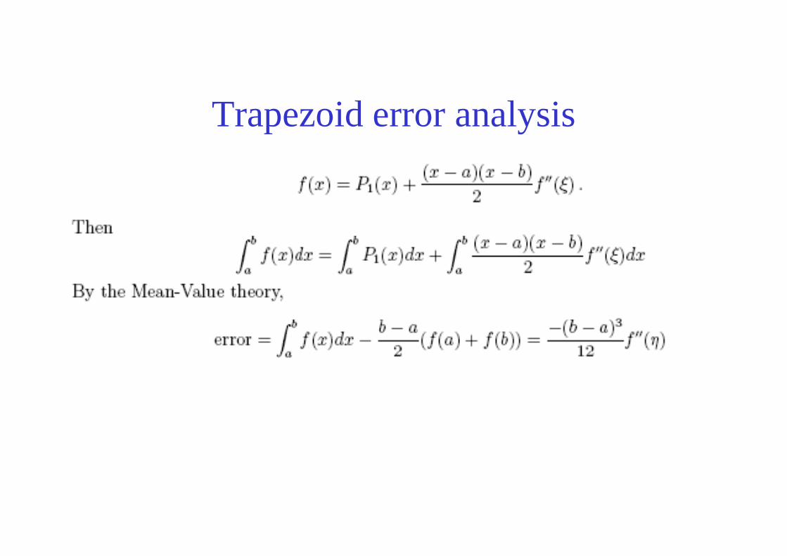
Trapezoid error analysis

Simpson’s rule error analysis

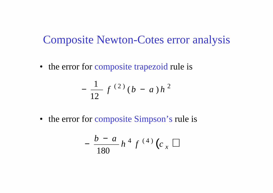
Composite Newton-Cotes error analysis

• the error for composite trapezoidrule is

2)2( )(12

1habf −−

• the error for composite Simpson’srule is

12

( )xcfhab )4(4

180

−−

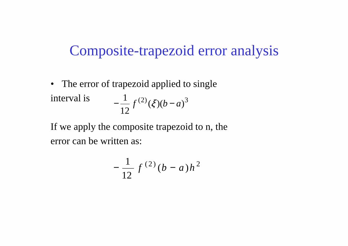
Composite-trapezoid error analysis

• The error of trapezoid applied to single

interval is

If we apply the composite trapezoid to n, the

3)2( ))((121

abf −− ξ

If we apply the composite trapezoid to n, the

error can be written as:

2)2( )(12

1habf −−

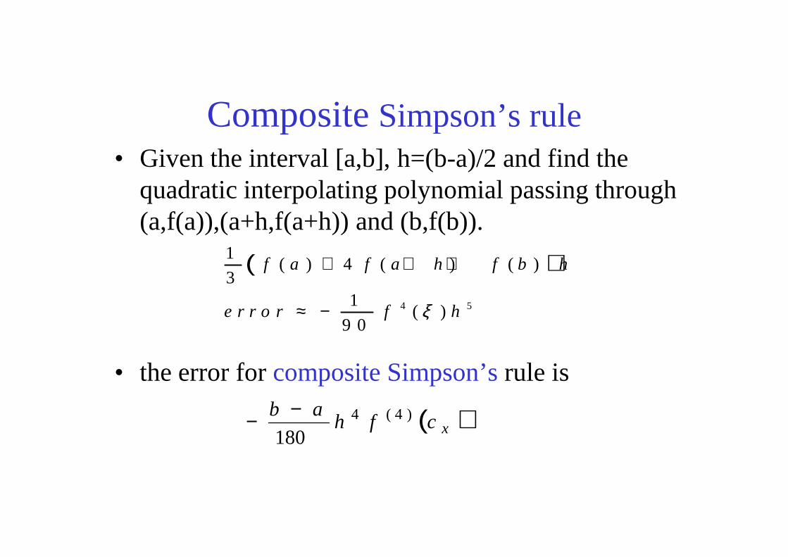
Composite Simpson’s rule• Given the interval [a,b], h=(b-a)/2 and find the

quadratic interpolating polynomial passing through (a,f(a)),(a+h,f(a+h)) and (b,f(b)).

( )1( ) 4 ( ) ( )

3f a f a h f b h+ + +

• the error for composite Simpson’srule is

4 5

31

( )9 0

e r r o r f hξ≈ −

( )xcfhab )4(4

180

−−

Gaussian Gaussian QuadraturesQuadratures• Newton-Cotes Formulae

– use evenly-spaced functional values

• Gaussian Quadratures– select functional values at non-uniformly – select functional values at non-uniformly

distributed points to achieve higher accuracy

– change of variables so that the interval of integration is [-1,1]

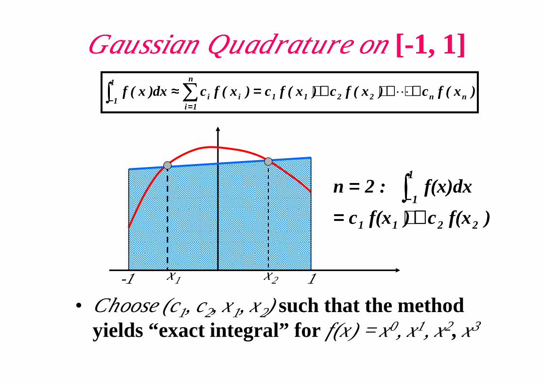
Gaussian Gaussian QuadratureQuadratureon on [[--11, , 11]]

)x(fc)x(fc)x(fc)x(fcdx)x(f nn2211i

1

1

n

1ii ++++++++++++====≈≈≈≈∫∫∫∫ ∑∑∑∑−−−−

====

L

f(x)dx :2n1

==== ∫∫∫∫−−−−

• Choose (c1, c2, x1, x2) such that the method yields “exact integral” for f(x) = x0, x1, x2, x3

)f(xc)f(xc

f(x)dx :2n

2211

1

++++======== ∫∫∫∫−−−−

x2x1-1 1

Gaussian Gaussian QuadratureQuadratureon on [[--11, , 11]]

Exact integral for f = x0, x1, x2, x3

– Four equations for four unknowns

)f(xc)f(xcf(x)dx :2n 2211

1

1++++======== ∫∫∫∫−−−−

========

++++========⇒⇒⇒⇒==== ∫∫∫∫−−−−

1c1ccc2dx1 1f 12

1

1 1

====

−−−−====

====

⇒⇒⇒⇒

++++========⇒⇒⇒⇒====

++++========⇒⇒⇒⇒====

++++========⇒⇒⇒⇒====

∫∫∫∫

∫∫∫∫

∫∫∫∫

∫∫∫∫

−−−−

−−−−

−−−−

−−−−

3

1x

3

1x

1c

xcxc0dxx xf

xcxc32

dxx xf

xcxc0xdx xf

2

1

2

322

31

1

1 133

222

21

1

1 122

221

1

1 1

1

)3

1(f)

3

1(fdx)x(fI

1

1++++−−−−======== ∫∫∫∫−−−−

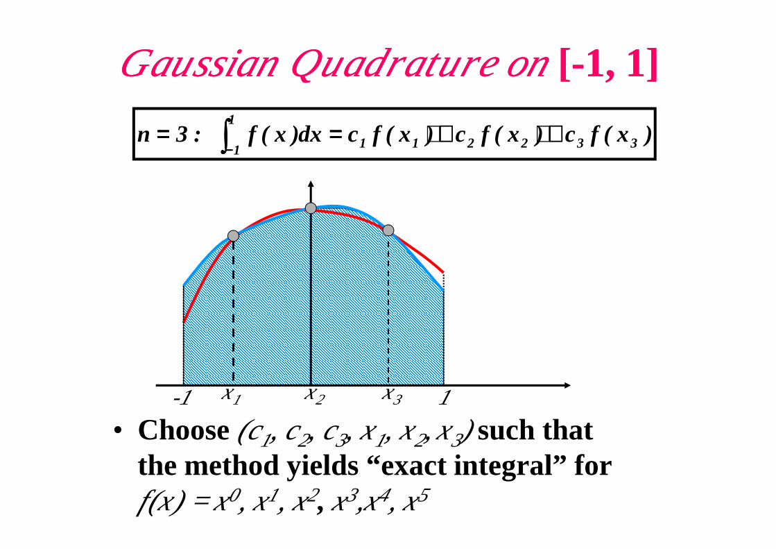
Gaussian Quadrature on Gaussian Quadrature on [[--11, , 11]]

)x(fc)x(fc)x(fcdx)x(f :3n 332211

1

1++++++++======== ∫∫∫∫−−−−

• Choose(c1, c2, c3, x1, x2, x3) such that the method yields “exact integral” for f(x) = x0, x1, x2, x3,x4, x5

x3x1-1 1x2

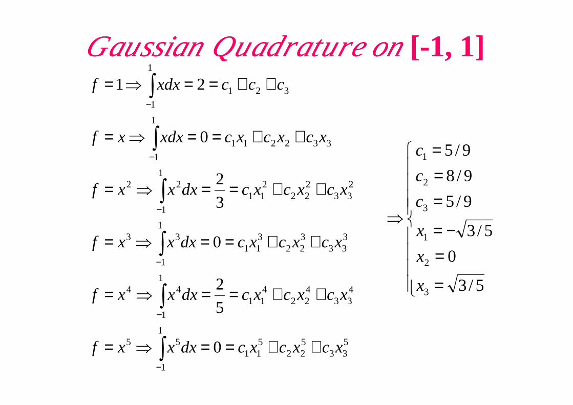
Gaussian Quadrature on Gaussian Quadrature on [[--11, , 11]]

233

222

211

122

332211

1

1

321

1

1

3

2

0

21

xcxcxcdxxxf

xcxcxcxdxxf

cccxdxf

++==⇒=

++==⇒=

++==⇒=

∫

∫

∫

−

−

===

9/5

9/8

9/5

3

2

1

c

c

c

533

522

511

1

1

55

433

422

411

1

1

44

333

322

311

1

1

33

1

0

5

2

0

3

xcxcxcdxxxf

xcxcxcdxxxf

xcxcxcdxxxf

++==⇒=

++==⇒=

++==⇒=

∫

∫

∫

∫

−

−

−

−

=

=−=

=⇒

5/3

0

5/3

9/5

3

2

1

3

x

x

x

c

Gaussian Quadrature on Gaussian Quadrature on [[--11, , 11]]

Exact integral for f = x0, x1, x2, x3, x4, x5

)53

(f95

)0(f98

)53

(f95

dx)x(fI1

1++++++++−−−−======== ∫∫∫∫−−−−

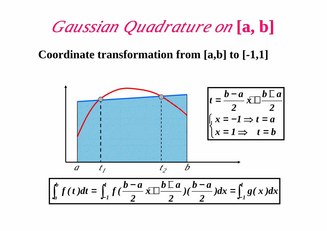
Gaussian Quadrature on Gaussian Quadrature on [a, b][a, b]

Coordinate transformation from [a,b] to [-1,1]

====⇒⇒⇒⇒−−−−====

++++++++−−−−====

at1x2

abx

2ab

t

t2t1a b

∫∫∫∫∫∫∫∫∫∫∫∫ −−−−−−−−====−−−−++++++++−−−−====

1

1

1

1

b

adx)x(gdx)

2ab

)(2

abx

2ab

(fdt)t(f

====⇒⇒⇒⇒========⇒⇒⇒⇒−−−−====

bt 1xat1x

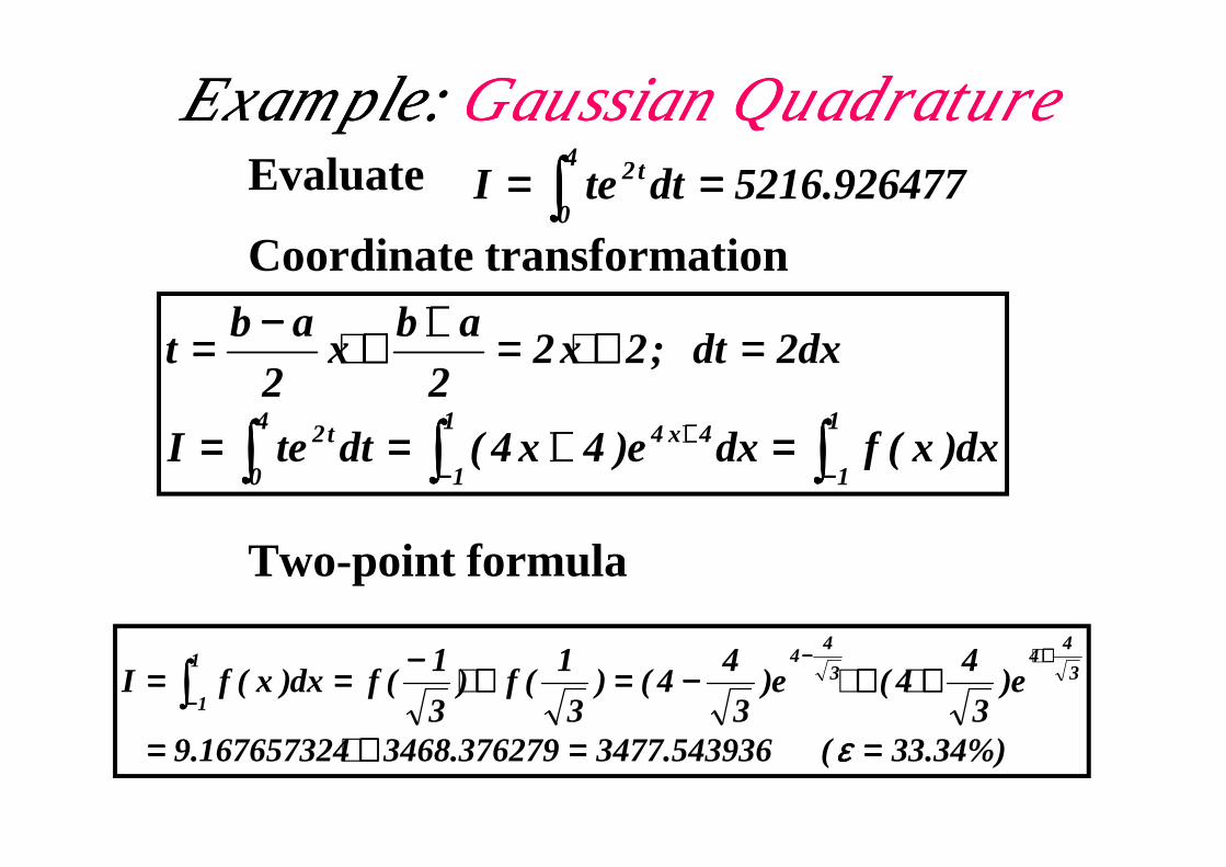
Example: Example: Gaussian QuadratureGaussian QuadratureEvaluate

Coordinate transformation

926477.5216dtteI4

0

t2 ======== ∫∫∫∫

∫∫∫∫∫∫∫∫∫∫∫∫++++ ====++++========

====++++====++++++++−−−−====11 4x44 t2 dx)x(fdxe)4x4(dtteI

2dxdt ;2x22

abx

2ab

t

Two-point formula

33.34%)( 543936.3477376279.3468167657324.9

e)3

44(e)

3

44()

3

1(f)

3

1(fdx)x(fI 3

44

3

441

1

========++++====

++++++++−−−−====++++−−−−========++++−−−−

−−−−∫∫∫∫εεεε

∫∫∫∫∫∫∫∫∫∫∫∫ −−−−−−−−

++++ ====++++========1

1

1

1

4x44

0

t2 dx)x(fdxe)4x4(dtteI

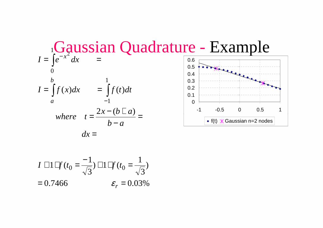
Gaussian Quadrature -Example

)(2

)()(1

1

1

0

2

=+−=

==

==

∫∫

∫

−

−

b

a

x

abxtwhere

dttfdxxfI

dxeI

00.10.20.30.40.50.6

-1 -0.5 0 0.5 1

%03.07466.0

)3

1(1)

3

1(1

)(2

00

==

=⋅+−=⋅≅

=

=−

+−=

r

tftfI

dxab

abxtwhere

ε

f(t) Gaussian n=2 nodes

Example: Example: Gaussian QuadratureGaussian QuadratureThree-point formula

)142689.8589(5

)3926001.218(8

)221191545.2(5

e)6.044(95

e)4(98

e)6.044(95

)6.0(f95

)0(f98

)6.0(f95

dx)x(fI

6.0446.04

1

1

++++++++====

++++++++++++−−−−====

++++++++−−−−========

++++−−−−

−−−−∫∫∫∫

Four-point formula

4.79%)( 106689.4967

)142689.8589(9

)3926001.218(9

)221191545.2(9

========

++++++++====

εεεε

[[[[ ]]]][[[[ ]]]]

%)37.0( 54375.5197 )339981.0(f)339981.0(f652145.0

)861136.0(f)861136.0(f34785.0dx)x(fI1

1

========++++−−−−++++++++−−−−======== ∫∫∫∫−−−−

εεεε

SummarySummary

• Integration Techniques– Trapezoidal Rule : Linear– Trapezoidal Rule : Linear– Simpson’s 1/3-Rule : Quadratic– Simpson’s 3/8-Rule : Cubic– Boole’s Rule : Fourth-order

• Gaussian Quadrature