Interpolation

Lagrange Interpolation

. .

.. .

(x ,f )

(x2,f2)

(x3,f3) (x4,f4)

(x5,f5)

f(x).(x1,f1) P(x)

f(x)

Introduction• The interpolation problem

– Given values of an unknown function f(x) at values x = x0, x1, …, xn, find approximate values of f(x) between these given values

• Polynomial interpolation– Find nth-order polynomial pn(x) that approximates the function f(x) and

provides exact agreement at the n node points:

)()(),()(),()( 1100 nnnnn xfxpxfxpxfxp === L

– The polynomial pn(x) is unique

– Interpolation: evaluate pn(x) for x0 <= x <= xn

– Extrapolation: evaluate pn(x) for x0 > x > xn

)()(),()(),()( 1100 nnnnn xfxpxfxpxfxp === L

Purposes for Interpolation

• Plotting smooth curve through discrete data points

• Quick and easy evaluation of mathematical function

• Replacing “difficult” function by “easy” one• Replacing “difficult” function by “easy” one

• “Reading between the lines” of table

• Differentiating or integrating tabular data

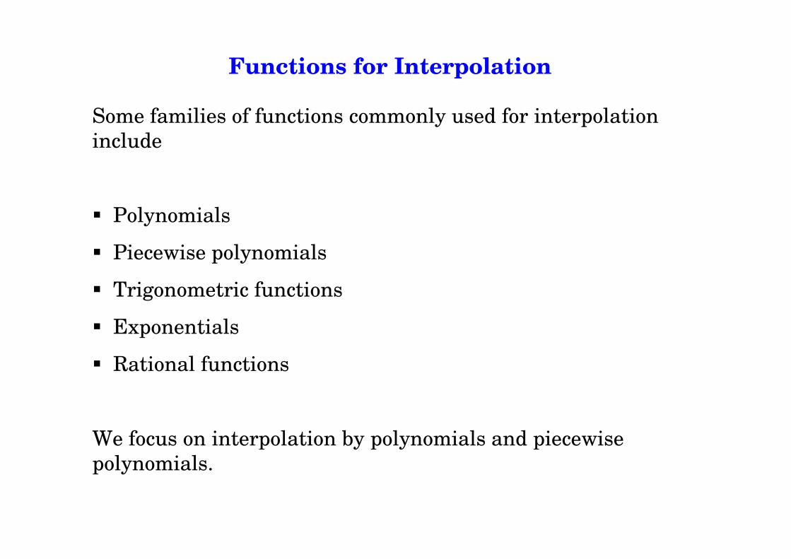
Functions for Interpolation

Some families of functions commonly used for interpolation

include

� Polynomials

� Piecewise polynomials

� Trigonometric functions� Trigonometric functions

� Exponentials

� Rational functions

We focus on interpolation by polynomials and piecewise

polynomials.

Polynomial Interpolation

)(...)()()( 2211 xuaxuaxuaxP mmm +++= )1(YAV =

V =

u x u x u x

u x u x u x

u x u x u x

n

n

n n n n

1 1 2 1 1

1 2 2 2 2

1 2

( ) ( ) ... ( )

( ) ( ) ... ( )

... ... ... ...

( ) ( ) ... ( )

Vandermonde matrix

n=m

miyxP iim ,...,2,1)( , ==A Y=

=

a

a

a

y

y

yn n

1

2

1

2

...,

...

YVA 1−=Extrapolation

Polynomial Interpolation

Simplest and commonest type of interpolation uses

polynomials.

Unique polynomial of degree at most n – 1 passes through n

data points (ti, yi), i = 1, . . . , n, where ti are distinct.

There are many ways to represent or compute polynomial, but

in theory all must give same result.in theory all must give same result.

Lagrange

Lagrange Interpolation

For given set of data points (ti, yi), i = 1, . . ., n,

Lagrange basis functions are given by

)x)...(xx)(xx)...(xx)(xx(x

)x)...(xx)(xx)...(xx)(xx(x(x)l

nj1jj1jj2j1j

n1j1j21

j −−−−−−−−−−

=+−

+−

)x(xn −

which means that matrix of linear system Ax = y is identity.

Thus, Lagrange polynomial interpolating data points (ti, yi) is

given by

pn–1 (t ) = y1l1 (t ) + y2l2 (t ) + ... + ynln (t ).

)x(x

)x(x

kj

kn

jk1,k −−

===π

Examples: Lagrange Interpolation

1-Use Lagrange interpolation to find interpolating polynomial

for three data points (–2, –27), (0, –1), 1, 0).

Lagrange polynomial of degree two interpolating three points

(t1, y1), (t2, y2), (t3, y3) is

.))(())(())((

)( 213

312

3212

tttty

tttty

ttttytp

−−−−+

−−−−+

−−−−= .

))(())(())(()(

23133

32122

312112 tttt

ytttt

ytttt

ytp−−

+−−

+−−

=

For this particular set of data, this becomes

.)1)(2(

)1)(2()1(

)12)(2(

)1(27)(2 −

−+−+−−−

−−= tttttp

2-Use Lagrange interpolation to find interpolating polynomial for

).sin()( xxf =

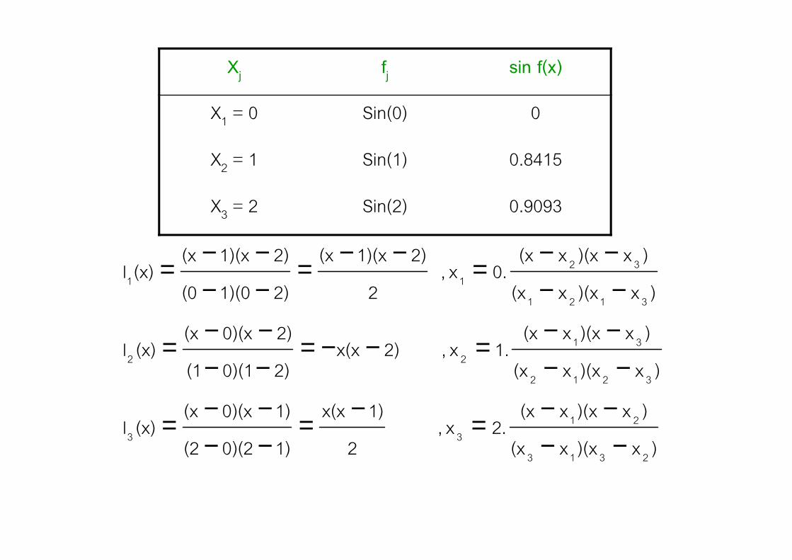
Lagrange InterpolationXj fj sin f(x)

X1 = 0 Sin(0) 0

X2 = 1 Sin(1) 0.8415

X3 = 2 Sin(2) 0.9093

)x)(xx(x

)x)(xx(x0.x,

2

2)1)(x(x

2)1)(0(0

2)1)(x(x(x)l 32

11 −−−−=−−=

−−−−=

)x)(xx(x

)x)(xx(x2.x,

2

1)x(x

1)0)(2(2

1)0)(x(x(x)l

)x)(xx(x

)x)(xx(x1.x, 2)x(x

2)0)(1(1

2)0)(x(x(x)l

)x)(xx(x0.x,

22)1)(0(0(x)l

2313

21

33

3212

31

22

3121

11

−−−−=−=

−−−−=

−−−−=−−=

−−−−=

−−==

−−=

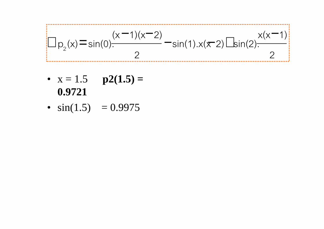
• x = 1.5 p2(1.5) =0.9721

• sin(1.5) = 0.9975

2

1)x(xsin(2).2)sin(1).x(x

2

2)1)(x(xsin(0).(x)p

2

−+−−−−=∴

Error in Interpolating a Function

If interpolation points are discrete sample of underlying

continuous function, then we may want to know how closely

interpolant approximates given function between sample

points.

If f is sufficiently smooth function, and pn–1 is unique

polynomial of degree at most n – 1 that interpolates f at n

points t1, . . . , tn, then points t1, . . . , tn, then

),())((!

)()()( 21

)(

1 n

n

n ttttttn

ftptf −−−=− − L

θ

where θ is some (unknown) point in interval [t1, tn].

Since point θ is unknown, this result is not particularly useful

unless we have bound on appropriate derivative of f, but it still

provides some insight into factors affecting accuracy of

polynomial interpolation.

• Take on and consider the error in linear interpolationto using nodes and satisfying

• We have:

Error in Interpolating a Function

( ) xexf = [ ]1.00x 1x

10 10 ≤≤≤ xx

( ) ( )( ) θexxxx

xPex

210

1−−

=−

( )xf

• 1-

• 2-

• We conclude

21

( )( ),

82

210

10

hxxxxMax

xxx=−−

≤≤

eeMaxxxx

=≤≤

θ

10

( ) eh

xPe x

8

2

1 =−

01 xxh −=

• Take on and consider the error in quadratic interpolationto using nodes satisfying

• We have:

Error in Interpolating a Function

( ) xexf = [ ]1.0( )xf 210 xandx,x

10 210 ≤≤≤≤ xxx

( ) ( )( )( ) θ2102

x e3!

xxxxxxxPe

−−−=−

• 1-

• 2-

• We conclude

eeMaxxxx

=≤≤

θ

10

3!( )( )( )

396

3210

10

hxxxxxxMax

xxx=

−−−≤≤

( ) 33

2 174.039

heh

xPe x ==−

0112 xxxxh −=−=

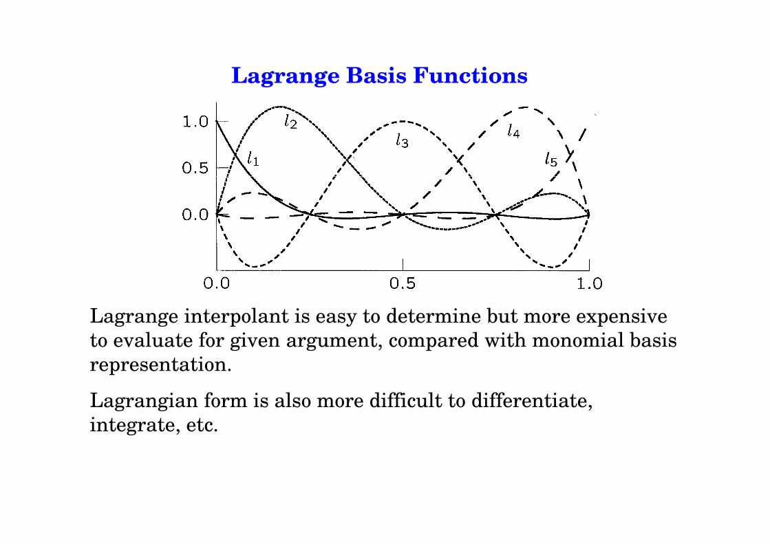
Lagrange Basis Functions

Lagrange interpolant is easy to determine but more expensive

to evaluate for given argument, compared with monomial basis

representation.

Lagrangian form is also more difficult to differentiate,

integrate, etc.

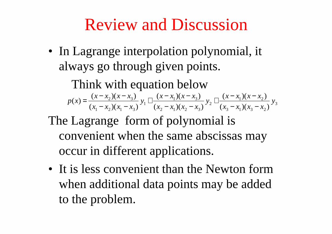
Review and Discussion

• In Lagrange interpolation polynomial, it always go through given points.

Think with equation below

The Lagrange form of polynomial is

32313

212

3212

311

3121

32

))((

))((

))((

))((

))((

))(()( y

xxxx

xxxxy

xxxx

xxxxy

xxxx

xxxxxp

−−−−+

−−−−+

−−−−=

The Lagrange form of polynomial is convenient when the same abscissas may occur in different applications.

• It is less convenient than the Newton form when additional data points may be added to the problem.

Newton

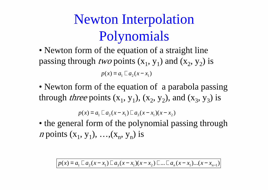
• Newton form of the equation of a straight line passing through two points (x1, y1) and (x2, y2) is

• Newton form of the equation of a parabola passing throughthree points (x, y ), (x , y ), and (x, y ) is

Newton Interpolation Polynomials

)()( 121 xxaaxp −+=

throughthree points (x1, y1), (x2, y2), and (x3, y3) is

• the general form of the polynomial passing through n points (x1, y1), …,(xn, yn) is

))(()()( 213121 xxxxaxxaaxp −−+−+=

))...((...))(()()( 11213121 −−−++−−+−+= nn xxxxaxxxxaxxaaxp

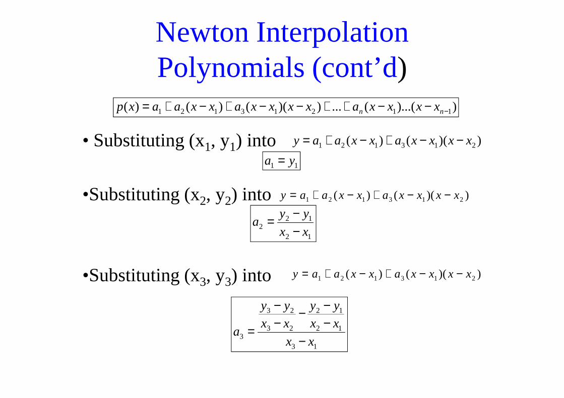
• Substituting (x1, y1) into

•Substituting (x2, y2) into

Newton Interpolation Polynomials (cont’d)

))(()( 213121 xxxxaxxaay −−+−+=

))(()( 213121 xxxxaxxaay −−+−+=

))...((...))(()()( 11213121 −−−++−−+−+= nn xxxxaxxxxaxxaaxp

11 ya =

•Substituting (x2, y2) into

•Substituting (x3, y3) into

))(()( 213121 xxxxaxxaay −−+−+=

))(()( 213121 xxxxaxxaay −−+−+=

12

122 xx

yya

−−=

13

12

12

23

23

3 xx

xx

yy

xx

yy

a−

−−−

−−

=

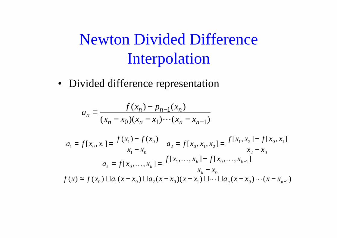
Newton Divided Difference Interpolation

• Divided difference representation

)())((

)()(

110

1

−

−−−−

−=nnnn

nnnn xxxxxx

xpxfa

L )())(( 110 −−−− nnnn xxxxxx L

)()())(()()()(

],,[],,[],,[

],[],[],,[

)()(],[

10102010

0

1010

02

10212102

01

01101

−

−

−−++−−+−+≈−

−==

−−==

−−==

nn

k

kkkk

xxxxaxxxxaxxaxfxfxx

xxfxxfxxfa

xx

xxfxxfxxxfa

xx

xfxfxxfa

LL

KKK

General form

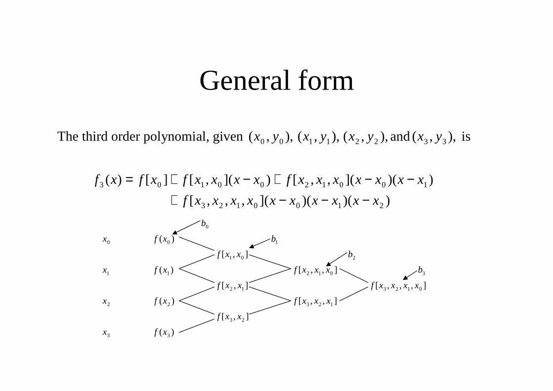
The third order polynomial, given ),,( 00 yx ),,( 11 yx ),,( 22 yx and ),,( 33 yx is

))()(](,,,[

))(](,,[)](,[][)( 1001200103

xxxxxxxxxxf

xxxxxxxfxxxxfxfxf

−−−+−−+−+=

))()(](,,,[ 2100123 xxxxxxxxxxf −−−+

0b

0x )( 0xf 1b

],[ 01 xxf 2b

1x )( 1xf ],,[ 012 xxxf 3b

],[ 12 xxf ],,,[ 0123 xxxxf

2x )( 2xf ],,[ 123 xxxf

],[ 23 xxf

3x )( 3xf

Newton Interpolation• Passing through the points (x1, y1)=(-2, 4),

(x2, y2)=(0, 2), and (x3, y3)=(2, 8).

• The equations is

• Where the coefficients are

)0))(2(())2(()( 321 −−−+−−+= xxaxaaxp

411 == ya

42−− yy• Where the coefficients are

•thus

1)2(0

42

12

122 −=

−−−=

−−=

xx

yya

1)2(2

)2(042

0228

13

12

12

23

23

3 =−−

−−−−

−−

=−

−−−

−−

=xx

xx

yy

xx

yy

a

2)2()2(4)( 2 ++=+++−= xxxxxxp

Newton Interpolation

• Passing through the points (x1, y1)=(-2, 4), (x2, y2)=(0, 2), and (x3, y3)=(2, 8).

))(()()( 213121 xxxxaxxaaxp −−+−+=

2)2()2(4)( 2 ++=+++−= xxxxxxp

Additional Data Points• We extend the previous example, adding the points(x4, y4) = (-1, -1) and (x5, y5) = (1, 1)

• Divided-difference • Divided-difference

table becomes

(with new entries

shown in bold)

• Newton interpolation

polynomial is )1)(2)(2()2)(2()2()2(4)( +−++−+−+++−= xxxxxxxxxxxp

Interpolating a Function

If interpolation points are discrete sample of underlying

continuous function, then we may want to know how closely

interpolant approximates given function between sample

points.

If f is sufficiently smooth function, and pn–1 is unique

polynomial of degree at most n – 1 that interpolates f at n

points t1, . . . , tn, then points t1, . . . , tn, then

),())((!

)()()( 21

)(

1 n

n

n ttttttn

ftptf −−−=− − L

θ

where θ is some (unknown) point in interval [t1, tn].

Since point θ is unknown, this result is not particularly useful

unless we have bound on appropriate derivative of f, but it still

provides some insight into factors affecting accuracy of

polynomial interpolation.

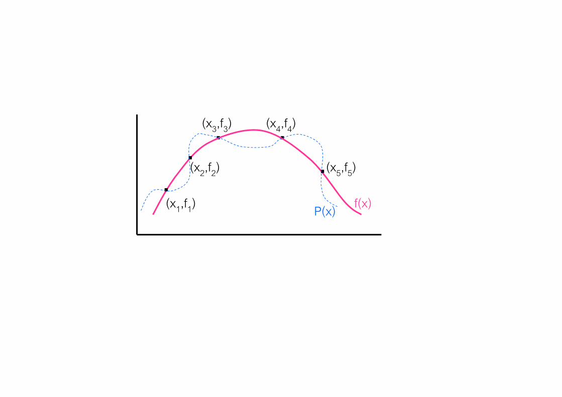
ExampleThe upward velocity of a rocket is given as a function of time in Table 1. Find the velocity at t=16 seconds using the Newton Divided Difference method for cubic interpolation.

t v(t)t v(t)

s m/s

0 0

10 227.04

15 362.78

20 517.35

22.5 602.97

30 901.67

Table 1: Velocity as a function of time

Figure 2: Velocity vs. time data for the rocket example

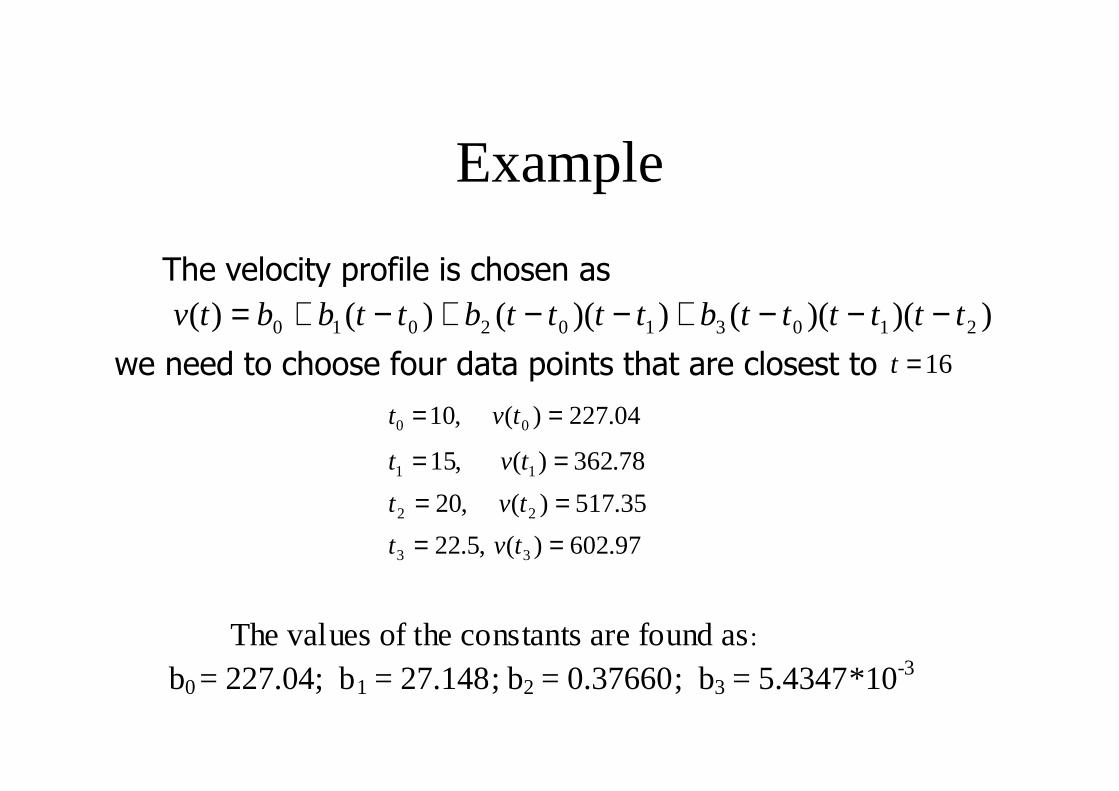
Example

The velocity profile is chosen as

))()(())(()()( 2103102010 ttttttbttttbttbbtv −−−+−−+−+=we need to choose four data points that are closest to 16=t

,100 =t 04.227)( 0 =tv

,151 =t 78.362)( 1 =tv ,202 =t 35.517)( 2 =tv ,5.223 =t 97.602)( 3 =tv

The values of the constants are found as: b0 = 227.04; b1 = 27.148; b2 = 0.37660; b3 = 5.4347*10-3

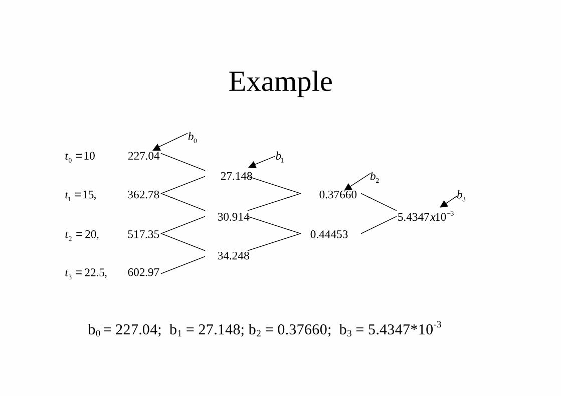
Example

0b

100 =t 04.227 1b

148.27 2b

,151 =t 78.362 37660.0 3b

b0 = 227.04; b1 = 27.148; b2 = 0.37660; b3 = 5.4347*10-3

,151 =t 78.362 37660.0 3b

914.30 3104347.5 −x

,202 =t 35.517 44453.0

248.34

,5.223 =t 97.602

Example

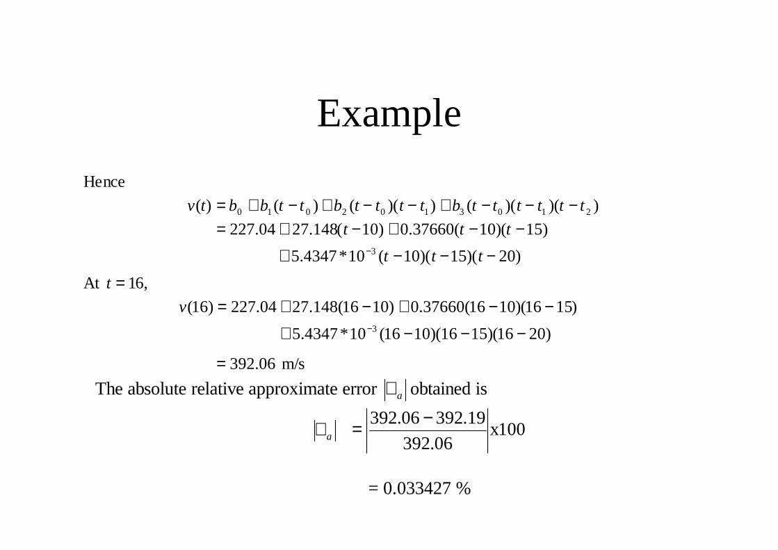
Hence

))()(())(()()( 2103102010 ttttttbttttbttbbtv −−−+−−+−+=

)20)(15)(10(10*4347.5

)15)(10(37660.0)10(148.2704.2273 −−−+

−−+−+=− ttt

ttt

At ,16=t At ,16=t

)2016)(1516)(1016(10*4347.5

)1516)(1016(37660.0)1016(148.2704.227)16(3 −−−+

−−+−+=−

v

06.392= m/s

The absolute relative approximate error a∈ obtained is

a∈ 100x06.392

19.39206.392 −=

= 0.033427 %

High-Degree Polynomial Interpolation

Interpolating polynomials of high degree are expensive to

determine and evaluate.

In some bases, coefficients of polynomial may be poorly

determined due to ill-conditioning of linear system to be solved.

High-degree polynomial necessarily has lots of “wiggles,” which

may bear no relation to data to be fit.may bear no relation to data to be fit.

Polynomial goes through required data points, but it may

oscillate wildly between data points.

Placement of Interpolation Points

Equally spaced interpolation points often yield unsatisfactory

results near ends of interval.

If points are bunched near ends of interval, more satisfactory

results are likely to be obtained with polynomial interpolation.

One way to accomplish this is to use Chebyshev points

)12( k = −−= π,,...,1,

2

)12(cos nk

n

ktk =

−−= π

on interval [–1, 1], or suitable transformation of these points

to arbitrary interval.

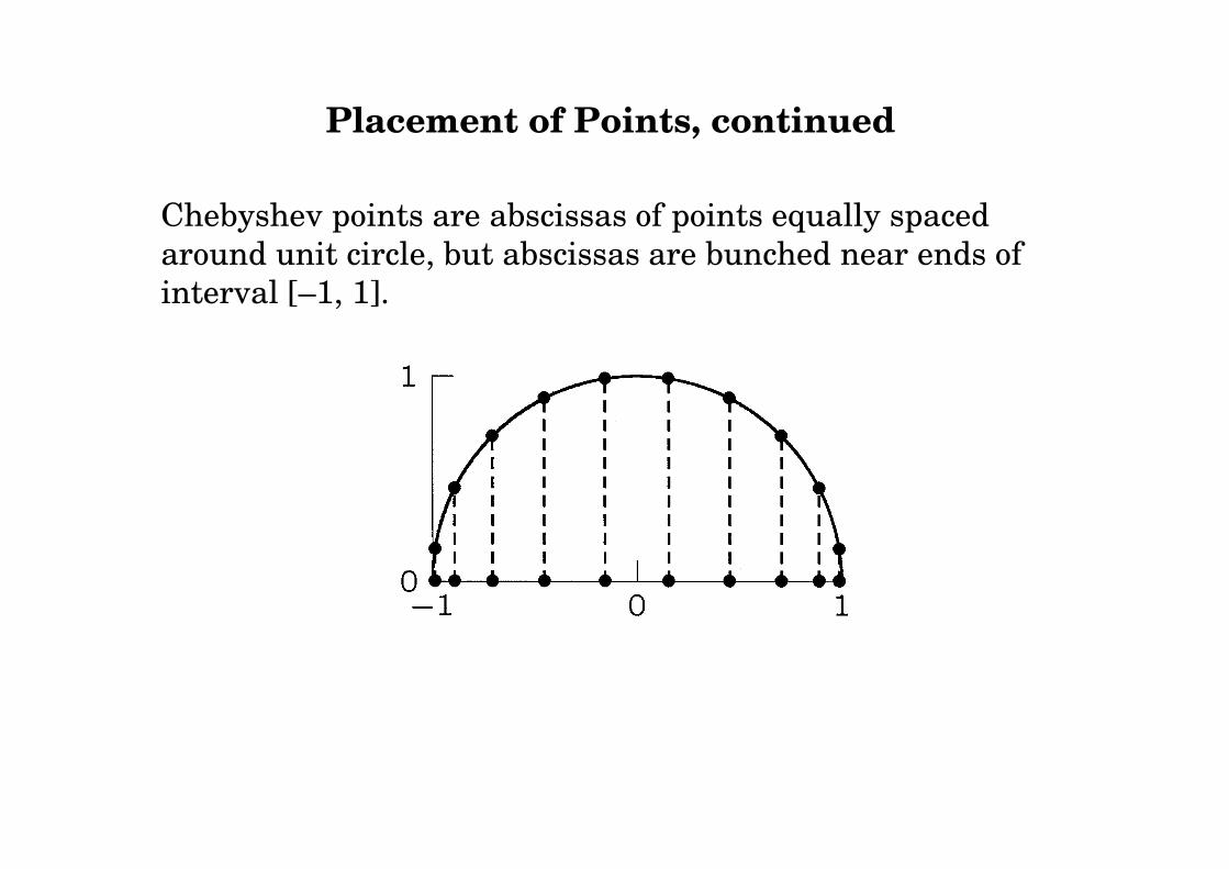
Placement of Points, continued

Chebyshev points are abscissas of points equally spaced

around unit circle, but abscissas are bunched near ends of

interval [–1, 1].