Numerical Integration

Aiichiro NakanoCollaboratory for Advanced Computing & Simulations

Department of Computer ScienceDepartment of Physics & Astronomy

Department of Chemical Engineering & Materials ScienceDepartment of Biological Sciences University of Southern California

Email: anakano@usc.eduNew toolbox: 1. Gaussian quadratures (orthogonal functions) 2. Newton’s method

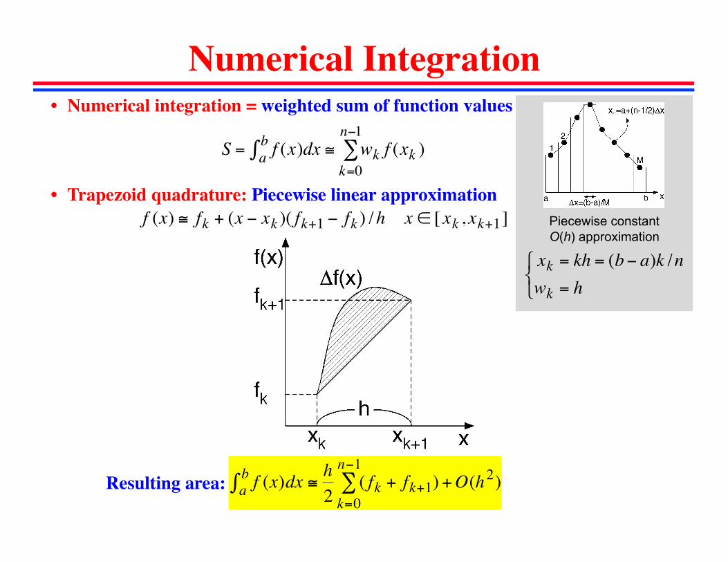
Numerical Integration• Numerical integration = weighted sum of function values

• Trapezoid quadrature: Piecewise linear approximation

€

S = f (x)dxab∫ ≅ wk f (xk )

k=0

n−1∑

€

f (x) ≅ fk + (x − xk )( fk+1 − fk ) /h x ∈ [ xk , xk+1]

€

f (x)dxab∫ ≅

h2

( fk + fk+1)k=0

n−1∑ +O(h2)Resulting area:

Piecewise constant O(h) approximation

€

xk = kh = (b− a)k /nwk = h⎧ ⎨ ⎩

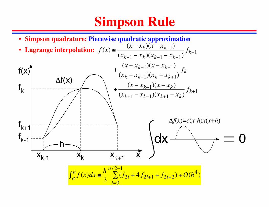
Simpson Rule• Simpson quadrature: Piecewise quadratic approximation • Lagrange interpolation:

€

f (x) ≅ (x − xk )(x − xk+1)(xk−1 − xk )(xk−1 − xk+1)

fk−1

+(x − xk−1)(x − xk+1)(xk − xk−1)(xk − xk+1)

fk

+(x − xk−1)(x − xk )

(xk+1 − xk−1)(xk+1 − xk )fk+1

€

f (x)dxab∫ ≅

h3

( f2l + 4 f2l+1 + f2l+2)l=0

n / 2−1∑ +O(h4 )

Δf(x)=c(x-h)x(x+h)

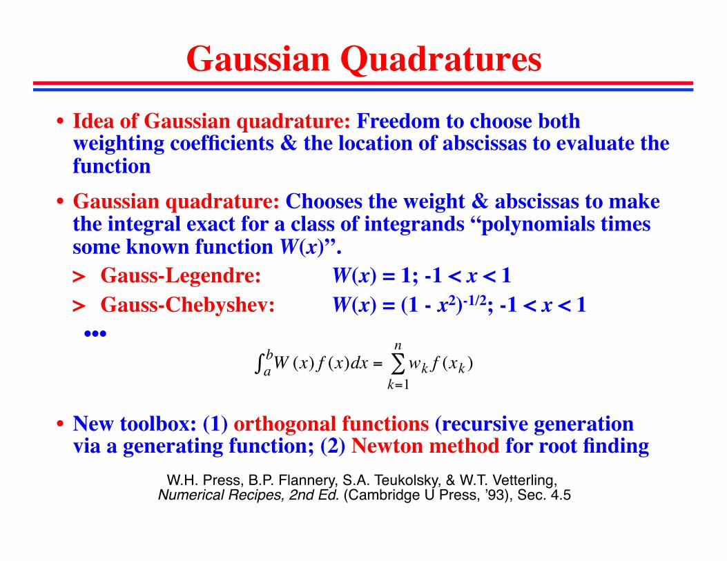
Gaussian Quadratures• Idea of Gaussian quadrature: Freedom to choose both

weighting coefficients & the location of abscissas to evaluate the function

• Gaussian quadrature: Chooses the weight & abscissas to make the integral exact for a class of integrands “polynomials times some known function W(x)”.> Gauss-Legendre: W(x) = 1; -1 < x < 1> Gauss-Chebyshev: W(x) = (1 - x2)-1/2; -1 < x < 1 •••

€

W (x) f (x)dxab∫ = wk f (xk )

k=1

n∑

W.H. Press, B.P. Flannery, S.A. Teukolsky, & W.T. Vetterling, !Numerical Recipes, 2nd Ed. (Cambridge U Press, ’93), Sec. 4.5!

• New toolbox: (1) orthogonal functions (recursive generation via a generating function; (2) Newton method for root finding

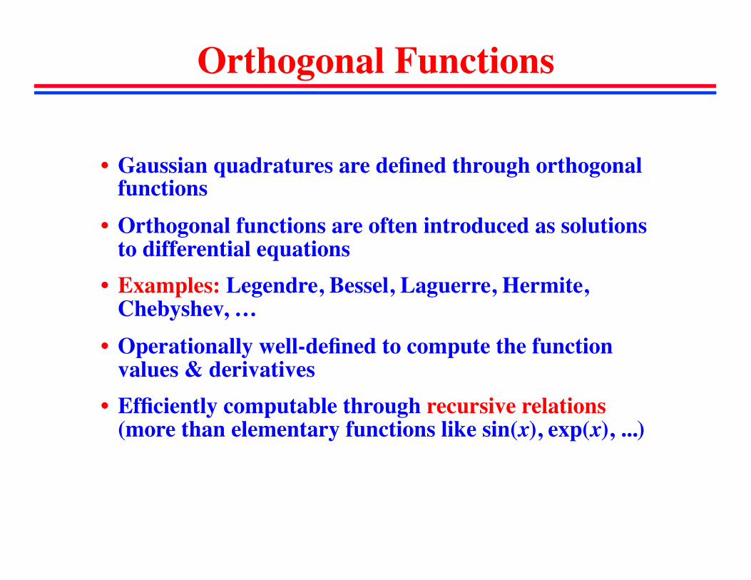
Orthogonal Functions

• Gaussian quadratures are defined through orthogonal functions

• Orthogonal functions are often introduced as solutions to differential equations

• Examples: Legendre, Bessel, Laguerre, Hermite, Chebyshev, …

• Operationally well-defined to compute the function values & derivatives

• Efficiently computable through recursive relations (more than elementary functions like sin(x), exp(x), ...)

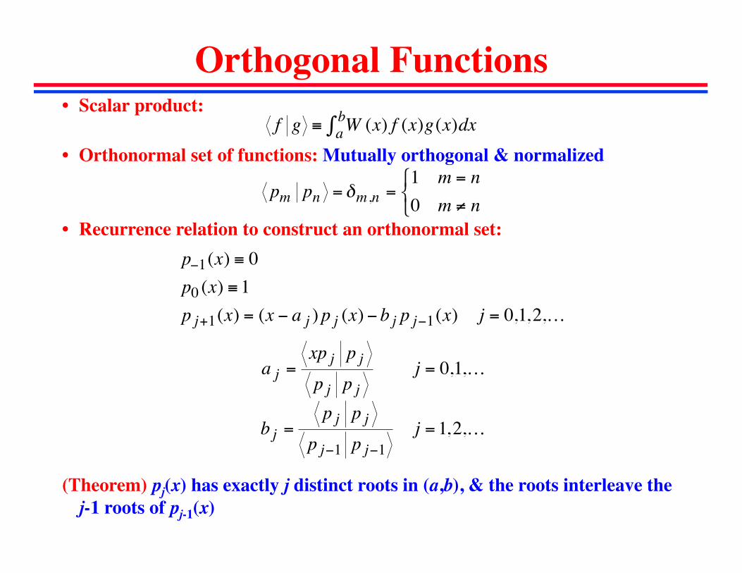
Orthogonal Functions• Scalar product:

• Orthonormal set of functions: Mutually orthogonal & normalized

• Recurrence relation to construct an orthonormal set:

(Theorem) pj(x) has exactly j distinct roots in (a,b), & the roots interleave the j-1 roots of pj-1(x)

€

f g ≡ W (x) f (x)g(x)dxab∫

€

pm pn = δm,n =1 m = n0 m ≠ n⎧ ⎨ ⎩

€

p−1(x) ≡ 0p0 (x) ≡ 1p j+1(x) = (x − a j )p j (x) − b j p j−1(x) j = 0,1,2,…

€

a j =xp j p jp j p j

j = 0,1,…

b j =p j p j

p j−1 p j−1j = 1,2,…

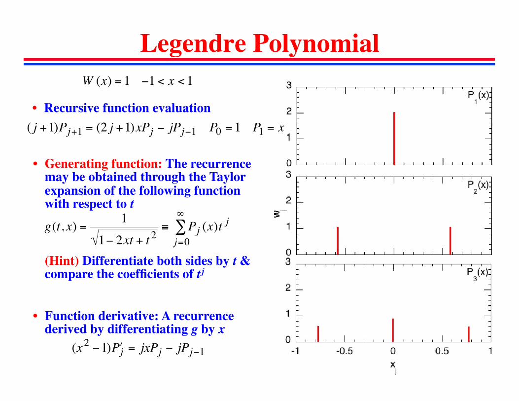
Legendre Polynomial

€

W (x) = 1 −1< x < 1

• Recursive function evaluation

• Function derivative: A recurrence derived by differentiating g by x

€

(x2 −1) ʹ P j = jxPj − jPj−1

• Generating function: The recurrence may be obtained through the Taylor expansion of the following function with respect to t

€

g(t, x) =1

1− 2xt + t 2≡ Pj (x)t

j

j=0

∞∑

€

( j +1)Pj+1 = (2 j +1)xPj − jPj−1 P0 = 1 P1 = x

(Hint) Differentiate both sides by t & compare the coefficients of t j

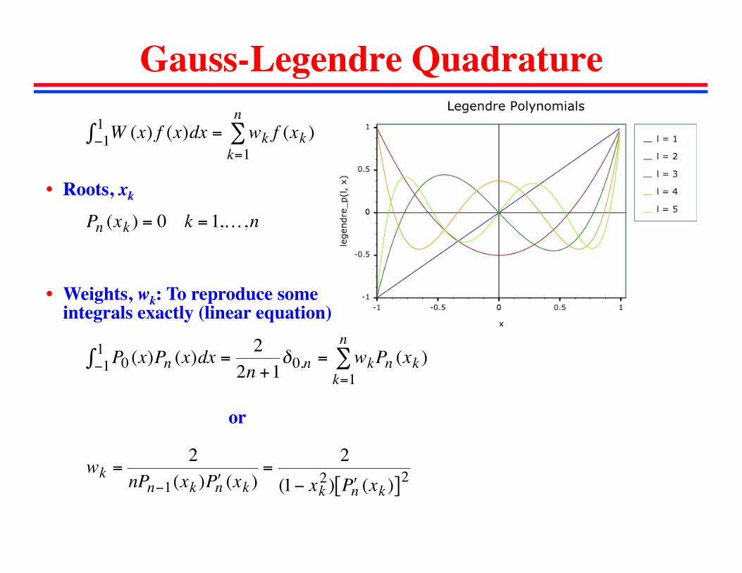
Gauss-Legendre Quadrature

• Roots, xk

• Weights, wk: To reproduce some integrals exactly (linear equation)

€

W (x) f (x)dx−11∫ = wk f (xk )

k=1

n∑

€

P0 (x)Pn (x)dx−11∫ =

22n +1

δ0,n = wkPn (xk )k=1

n∑

€

wk =2

nPn−1(xk ) ʹ P n (xk )=

2(1− xk

2) ʹ P n (xk )[ ]2

€

Pn (xk ) = 0 k = 1,…,n

or

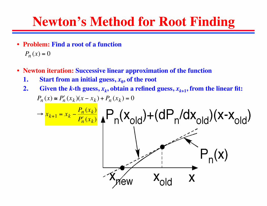
Newton’s Method for Root Finding

€

Pn (x) = 0• Problem: Find a root of a function

• Newton iteration: Successive linear approximation of the function1. Start from an initial guess, x0, of the root2. Given the k-th guess, xk, obtain a refined guess, xk+1, from the linear fit:

€

Pn (x) ≅ ʹ P n (xk )(x − xk ) + Pn (xk ) = 0

€

→ xk+1 = xk −Pn (xk )ʹ P n (xk )

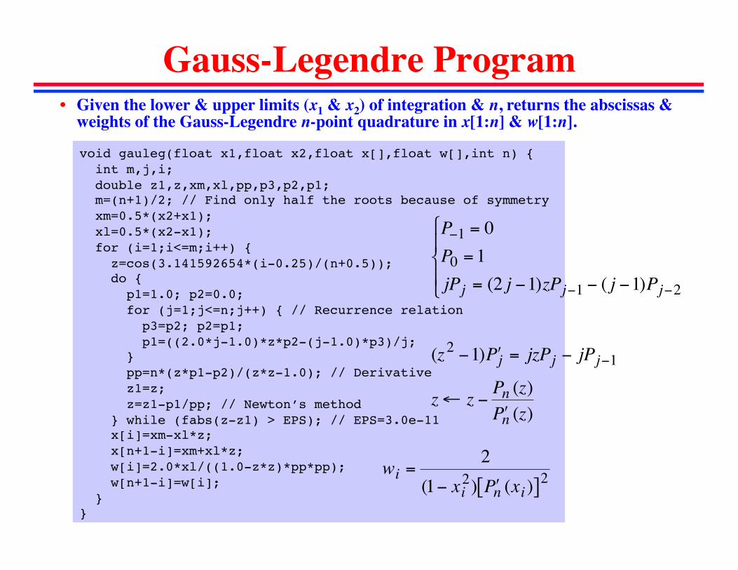
Gauss-Legendre Program

void gauleg(float x1,float x2,float x[],float w[],int n) { ! int m,j,i; ! double z1,z,xm,xl,pp,p3,p2,p1; ! m=(n+1)/2; // Find only half the roots because of symmetry! xm=0.5*(x2+x1); ! xl=0.5*(x2-x1); ! for (i=1;i<=m;i++) { ! z=cos(3.141592654*(i-0.25)/(n+0.5)); ! do { ! p1=1.0; p2=0.0; ! for (j=1;j<=n;j++) { // Recurrence relation ! p3=p2; p2=p1; ! p1=((2.0*j-1.0)*z*p2-(j-1.0)*p3)/j; ! } ! pp=n*(z*p1-p2)/(z*z-1.0); // Derivative ! z1=z; ! z=z1-p1/pp; // Newton’s method ! } while (fabs(z-z1) > EPS); // EPS=3.0e-11 ! x[i]=xm-xl*z; ! x[n+1-i]=xm+xl*z; ! w[i]=2.0*xl/((1.0-z*z)*pp*pp); ! w[n+1-i]=w[i]; ! } !}!

• Given the lower & upper limits (x1 & x2) of integration & n, returns the abscissas & weights of the Gauss-Legendre n-point quadrature in x[1:n] & w[1:n]. !

€

z← z − Pn (z)ʹ P n (z)

€

P−1 = 0P0 = 1jPj = (2 j −1)zPj−1 − ( j −1)Pj−2

⎧

⎨ ⎪

⎩ ⎪

€

(z2 −1) ʹ P j = jzPj − jPj−1

€

wi =2

(1− xi2) ʹ P n (xi )[ ]2

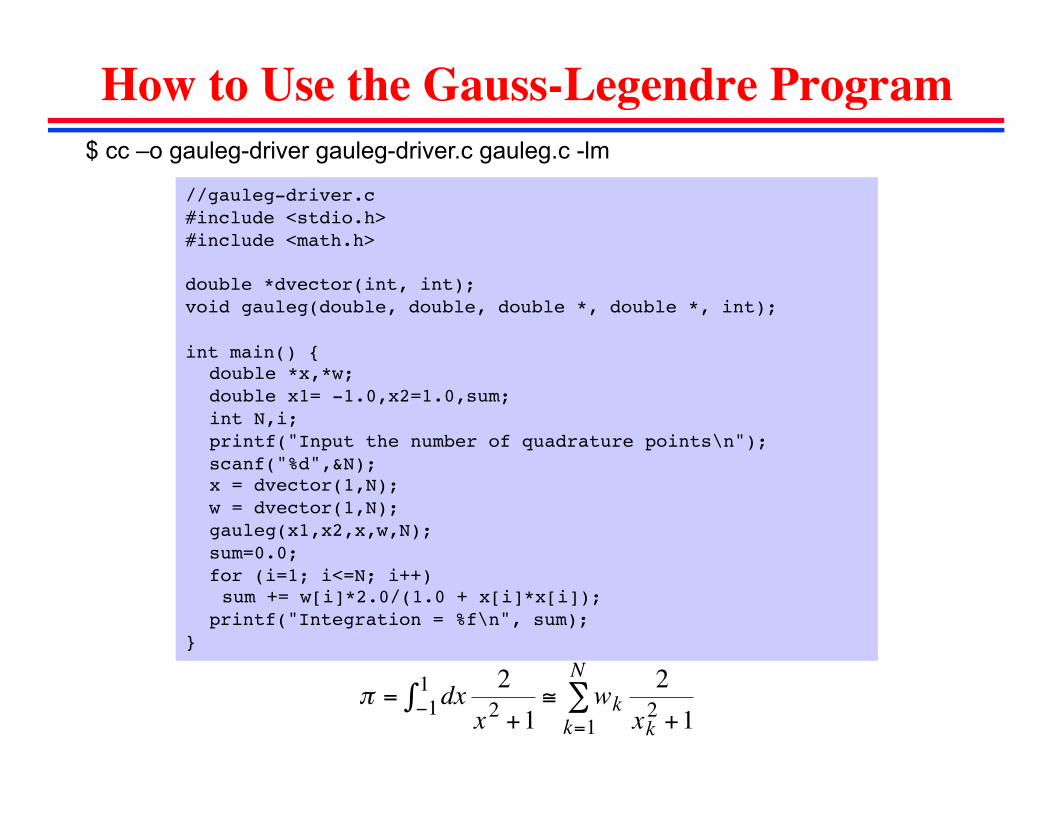
How to Use the Gauss-Legendre Program

//gauleg-driver.c!#include <stdio.h>!#include <math.h>!

double *dvector(int, int);!void gauleg(double, double, double *, double *, int);!

int main() {!!double *x,*w;!!double x1= -1.0,x2=1.0,sum;!!int N,i;!!printf("Input the number of quadrature points\n");!!scanf("%d",&N);!!x = dvector(1,N);!!w = dvector(1,N);!!gauleg(x1,x2,x,w,N);!!sum=0.0;!!for (i=1; i<=N; i++)!!!sum += w[i]*2.0/(1.0 + x[i]*x[i]);!!printf("Integration = %f\n", sum);!

}!

$ cc –o gauleg-driver gauleg-driver.c gauleg.c -lm

€

π = dx 2x2 +1−1

1∫ ≅ wk2

xk2 +1k=1

N∑

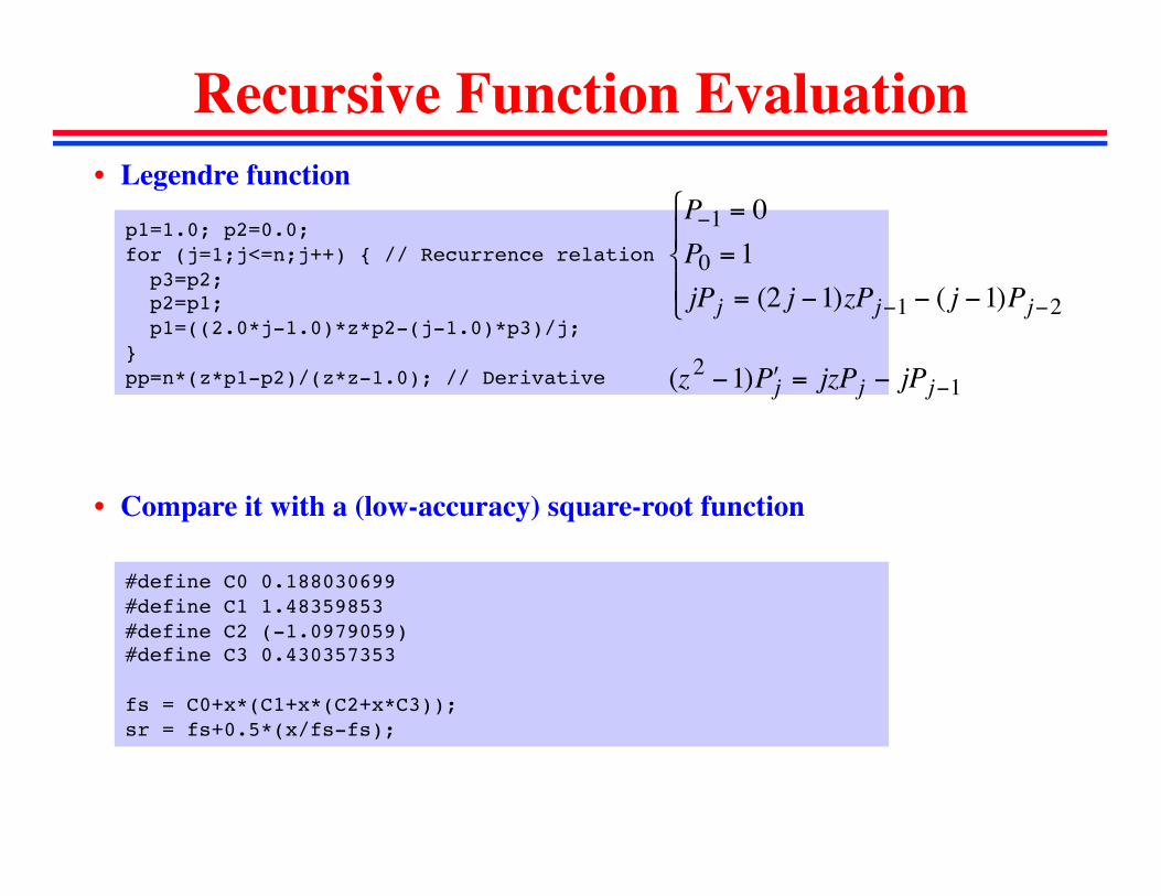
Recursive Function Evaluation

p1=1.0; p2=0.0; !for (j=1;j<=n;j++) { // Recurrence relation ! p3=p2;! p2=p1; ! p1=((2.0*j-1.0)*z*p2-(j-1.0)*p3)/j; !} !pp=n*(z*p1-p2)/(z*z-1.0); // Derivative !

• Legendre function!

€

P−1 = 0P0 = 1jPj = (2 j −1)zPj−1 − ( j −1)Pj−2

⎧

⎨ ⎪

⎩ ⎪

€

(z2 −1) ʹ P j = jzPj − jPj−1

#define C0 0.188030699!#define C1 1.48359853!#define C2 (-1.0979059)!#define C3 0.430357353!

fs = C0+x*(C1+x*(C2+x*C3));!sr = fs+0.5*(x/fs-fs);!

• Compare it with a (low-accuracy) square-root function!