Embed Size (px)
Citation preview
1
Civil Engineering Computation Ordinary Differential Equations
March 21, 1857 – An earthquake in Tokyo, Japan kills over 100,000.
2
Contents
Basic idea Euler’s method Improved Euler method Second order equations 4th order Runge-Kutta method Two-point boundary value problems Cash-Karp Runge-Kutta method Ordinary differential equation methods
and numerical integration
2
3
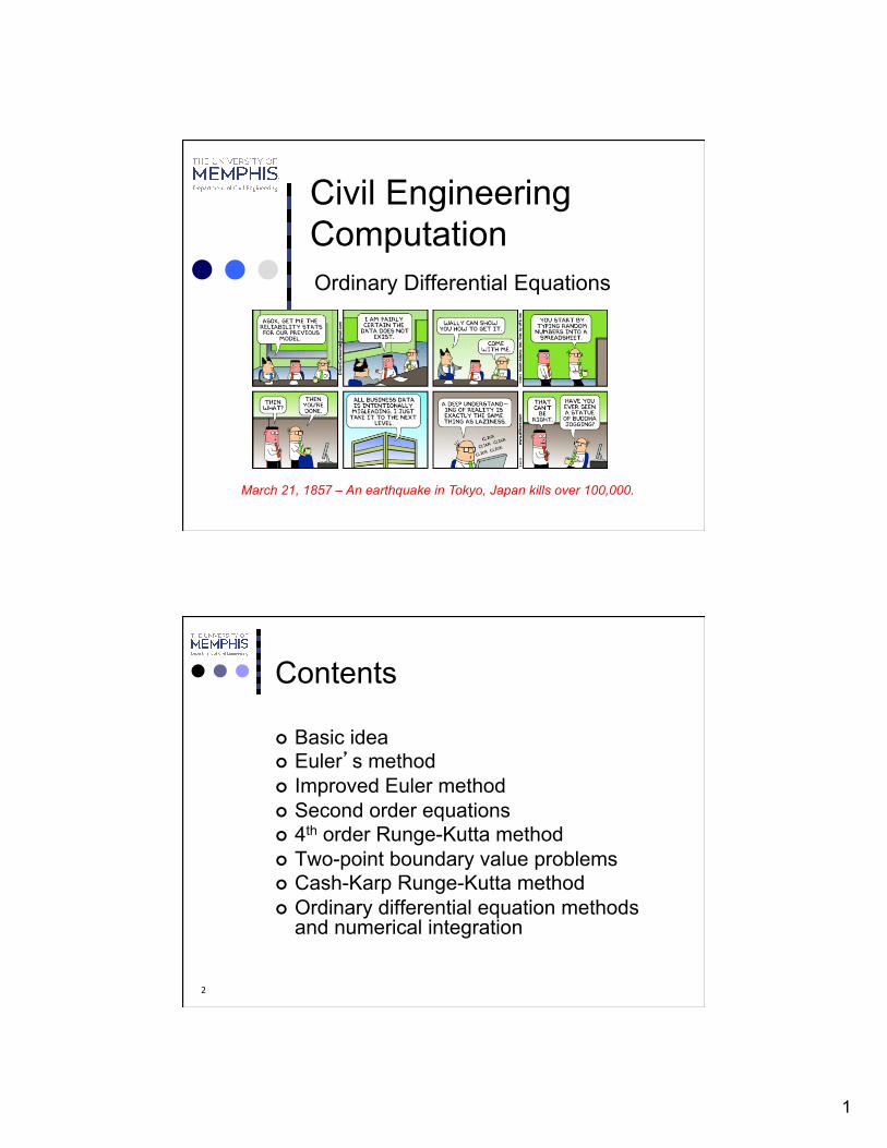
Example Problem
Vehicle with forward force F and drag force D
From Newton’s Second Law,
F – D = m dV/dt
Drag is approximately proportional to V2 so D = cV2
4
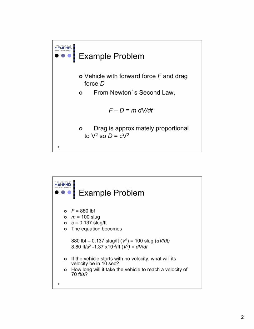
Example Problem
F = 880 lbf m = 100 slug c = 0.137 slug/ft The equation becomes
880 lbf – 0.137 slug/ft (V2) = 100 slug (dV/dt) 8.80 ft/s2 -1.37 x10⁻³/ft (V2) = dV/dt
If the vehicle starts with no velocity, what will its
velocity be in 10 sec? How long will it take the vehicle to reach a velocity of
70 ft/s?

3
5
Sample Diff. Equation
880 lbf – 0.137 slug/ft (V2) = 100 slug (dV/dt) 8.80 ft/s2 -1.37 x10⁻³/ft (V2) = dV/dt
Integrating both sides after isolating the variables
This is a closed form solution which can be manipulated and used to solve the questions posed.
If the vehicle starts with no velocity, what will its velocity be in 10 sec?
How long will it take the vehicle to reach a velocity of 70 ft/s?
Example Problem
Locating Roots Numerically 6
0
10
20
30
40
50
60
70
80
90
0 5 10 15 20 25 30 35
Velo
city
(fps
)
Time (seconds)
Velocity Profile
4
Example Problem
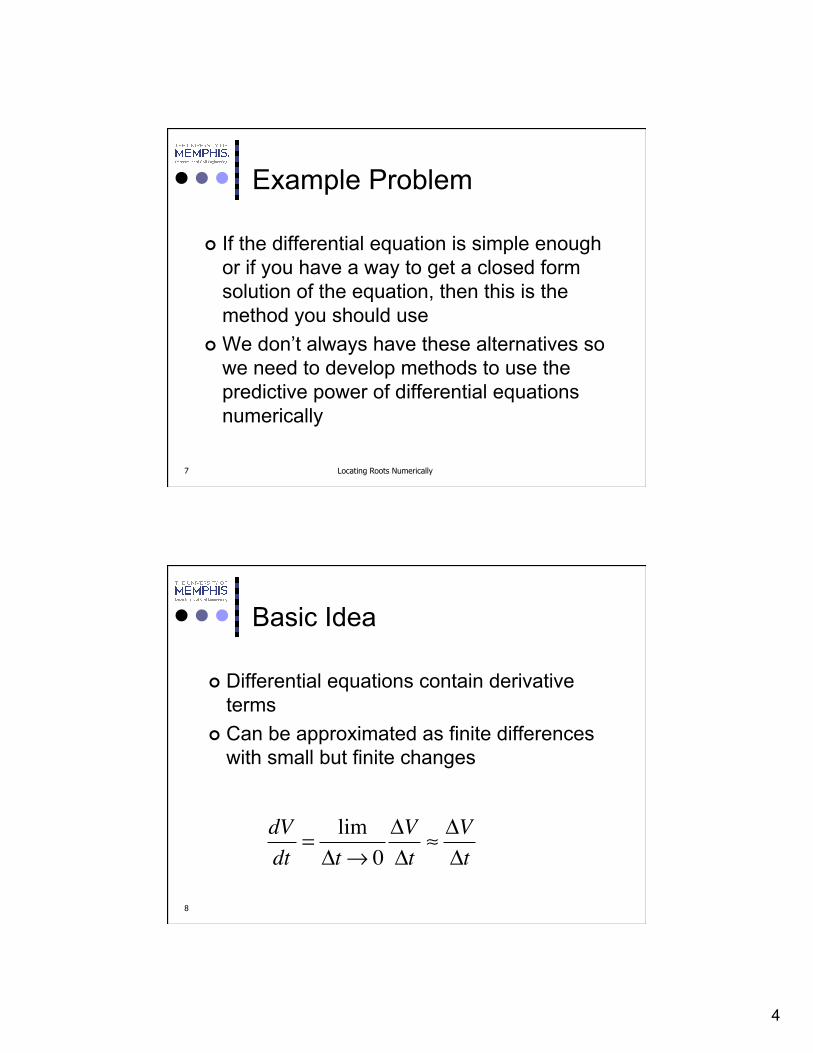
If the differential equation is simple enough or if you have a way to get a closed form solution of the equation, then this is the method you should use
We don’t always have these alternatives so we need to develop methods to use the predictive power of differential equations numerically
Locating Roots Numerically 7
8
Basic Idea
Differential equations contain derivative terms
Can be approximated as finite differences with small but finite changes dV
dt= lim!t" 0
!V!t
# !V!t

5
9
Euler’s Method
dV/dt ≈ ∆V/∆t
∆V ≈ dV/dt * ∆t
∆V = V(t+∆t) - V(t)
(8.1.1) V(t+∆t) =V(t) + dV/dt * ∆t
This is Euler’s method
10
Compare Euler’s Method, Taylor Series
Taylor series: V(t+∆t) =V(t) + dV/dt *∆t + d2V/dt2*∆t 2+ higher terms
Euler’s method agrees with series through 1st derivative term
So Euler ‘s called first order method

6
11
Euler’s Method
If we know the value of the function at t and the rate of change of the function at t, we can predict the value of the function at some step Δt beyond t.
f t + !t( ) = f t( )+ "f t( )!tf tn+1( ) = f tn( )+ "f tn( ) tn+1 # tn( )
12
Euler’s Method
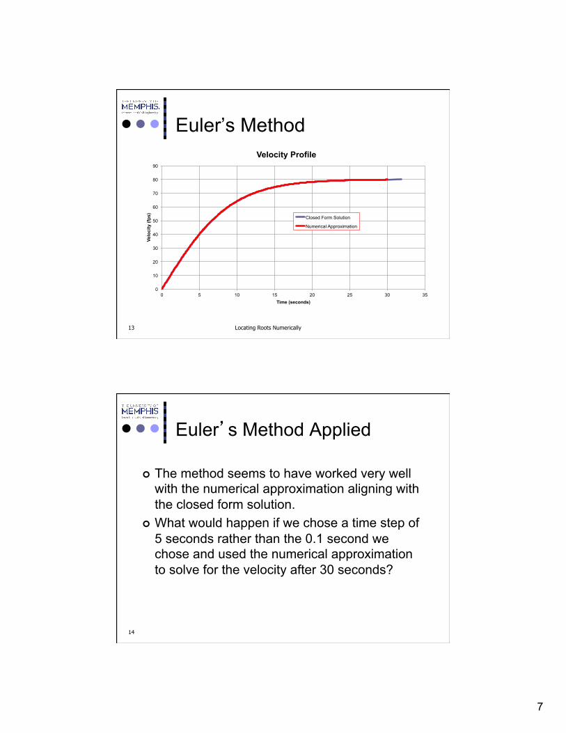
We can take the example problem and select a time step (delta t) of 0.1 sec and calculate a velocity profile using the Euler method.
f t + !t( ) = f t( )+ "f t( )!tf tn+1( ) = f tn( )+ "f tn( ) tn+1 # tn( )
7
Euler’s Method
Locating Roots Numerically 13
0
10
20
30
40
50
60
70
80
90
0 5 10 15 20 25 30 35
Velo
city
(fps
)
Time (seconds)
Velocity Profile
Closed Form Solution
Numerical Approximation
14
Euler’s Method Applied
The method seems to have worked very well with the numerical approximation aligning with the closed form solution.
What would happen if we chose a time step of 5 seconds rather than the 0.1 second we chose and used the numerical approximation to solve for the velocity after 30 seconds?

8
Locating Roots Numerically 15
0
10
20
30
40
50
60
70
80
90
0 5 10 15 20 25 30 35
Velo
city
(fps
)
Time (seconds)
Velocity Profile
Closed Form Solution
"0.1 second time step"
"5 second time step"
16
Euler’s Method Applied
While the method with a time step of 5 seconds did give you a fairly good answer at 30 seconds at intermediate points the answer wasn’t as good.
This is actually a very well behaved function, most functions would have an even greater error if we choose too great a time step.
9
17
Euler’s Method Applied
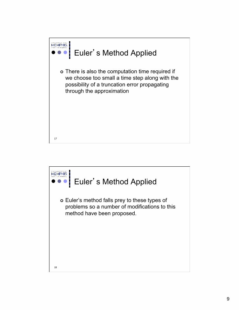
There is also the computation time required if we choose too small a time step along with the possibility of a truncation error propagating through the approximation
18
Euler’s Method Applied
Euler’s method falls prey to these types of problems so a number of modifications to this method have been proposed.
10
19
Improved Euler Method (Heun’s Method)
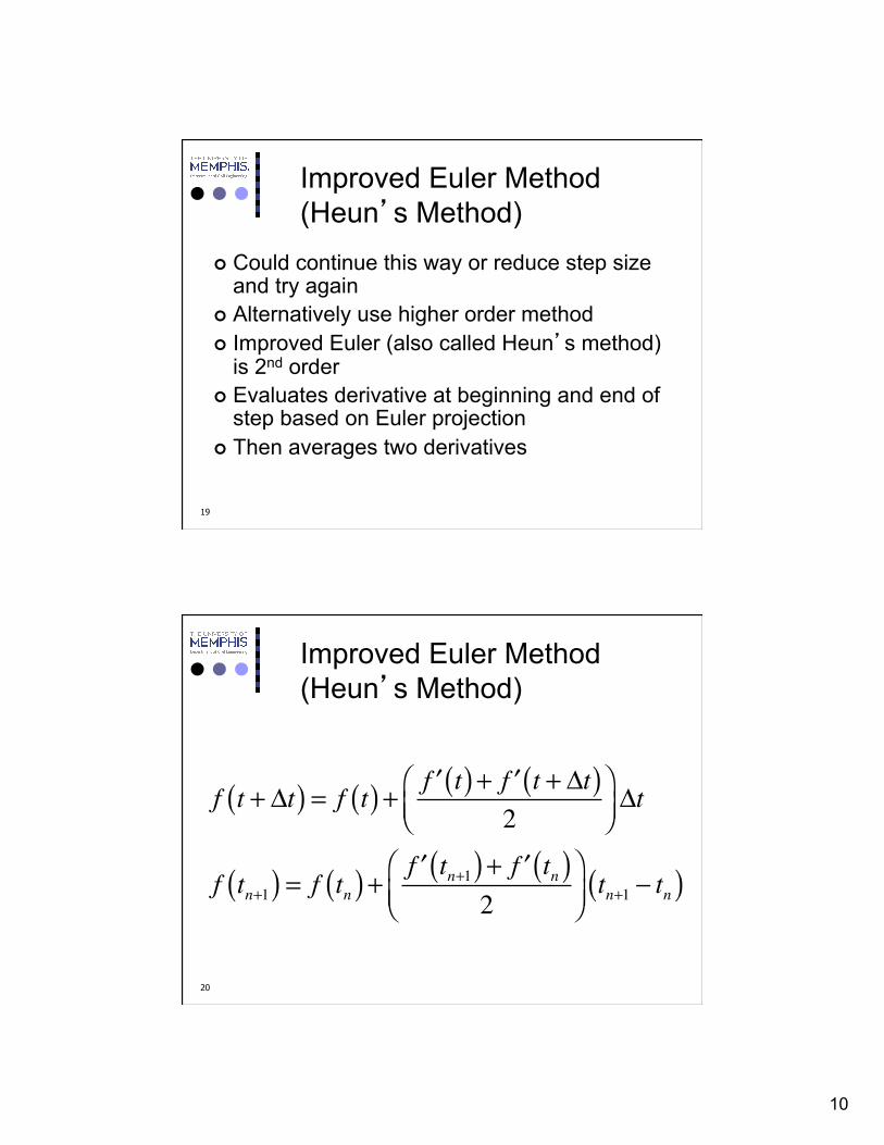
Could continue this way or reduce step size and try again
Alternatively use higher order method Improved Euler (also called Heun’s method)
is 2nd order Evaluates derivative at beginning and end of
step based on Euler projection Then averages two derivatives
20
Improved Euler Method (Heun’s Method)
f t + !t( ) = f t( )+ "f t( )+ "f t + !t( )2
#$%
&'(!t
f tn+1( ) = f tn( )+ "f tn+1( )+ "f tn( )2
#$%
&'(tn+1 ) tn( )

11
21
Improved Euler Method (Heun’s Method)
0
10
20
30
40
50
60
70
80
90
0 5 10 15 20 25 30 35
Velo
city
(fps
)
Time (seconds)
Velocity Profile
Closed Form Solution
"0.1 second time step"
"5 second time step"
Heun 1 second time step
22
Generalize for Second Order Equations
Could have written dV/dt as d(dx/dt))/dt = d2x/dt2
Then original V equation could be written as: d2x/dt2 = 8.80 – 1.37x10⁻³*(dx/dt)2
A second order equation in x

12
23
But our methods solve only first order equations
Instead of solving second order equation make 2 first order equations and solve together
dx/dt = g(x,v,t) and dV/dt = f(x,v,t) (In example V equation did not depend on x.
In general equations will be mutually dependent.)
Generalize for Second Order Equations
24
In this case dx/dt and dV/dt both had physical meaning.
If dx/dt did not have physical meaning we would still have to create equation for it in terms of solution to second derivative equation – name for your favorite variable
Similarly a 3rd order equation would be broken up into 3 first order equations
Generalize for Second Order Equations
13
25
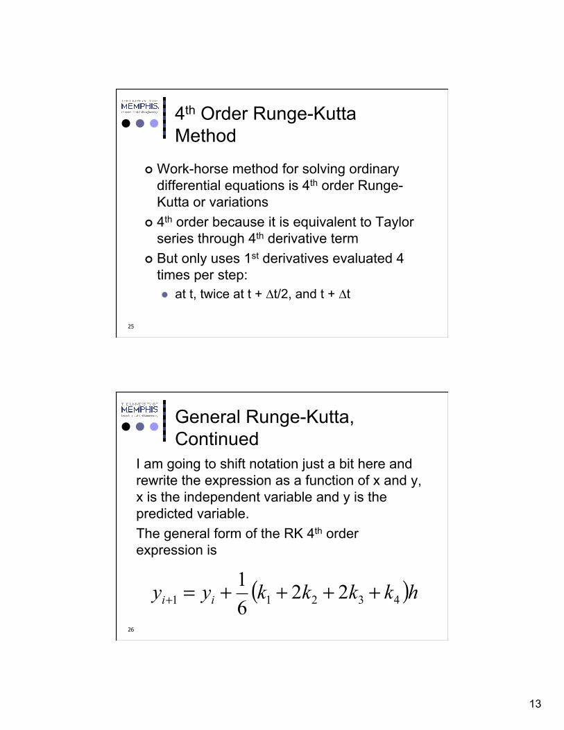
4th Order Runge-Kutta Method
Work-horse method for solving ordinary differential equations is 4th order Runge-Kutta or variations
4th order because it is equivalent to Taylor series through 4th derivative term
But only uses 1st derivatives evaluated 4 times per step: at t, twice at t + ∆t/2, and t + ∆t
26
General Runge-Kutta, Continued
I am going to shift notation just a bit here and rewrite the expression as a function of x and y, x is the independent variable and y is the predicted variable. The general form of the RK 4th order expression is
( )hkkkkyy ii 43211 2261 ++++=+
14
27
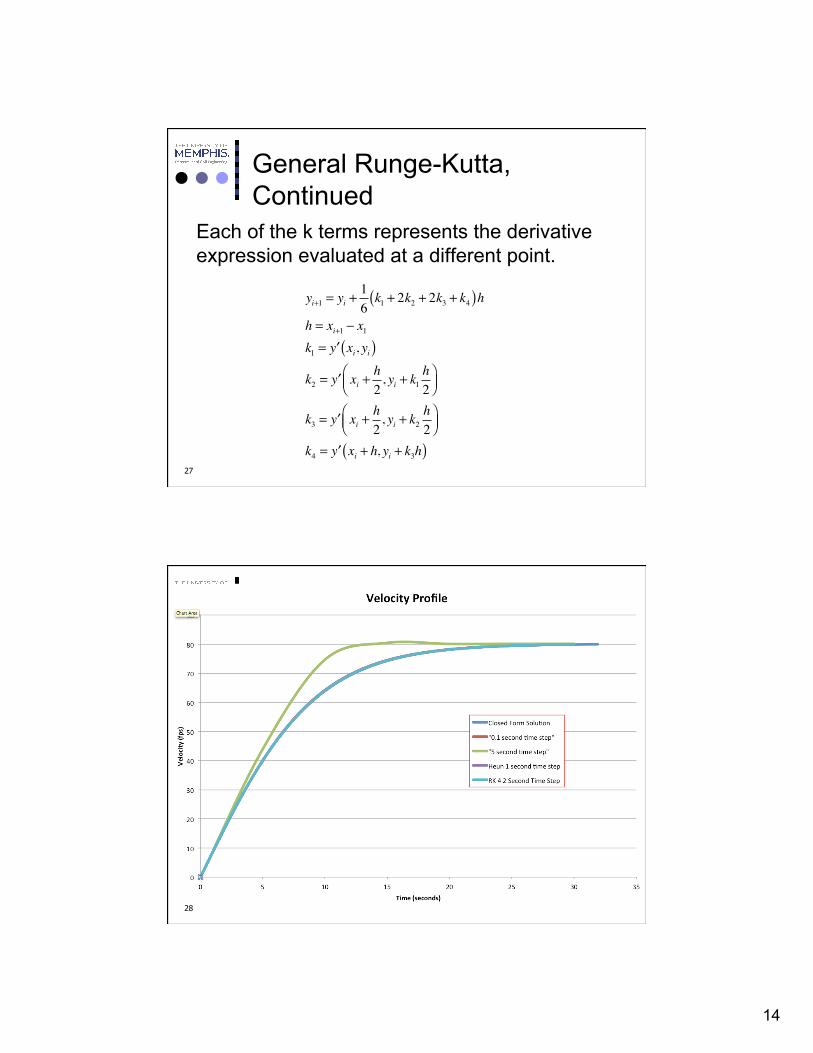
General Runge-Kutta, Continued
Each of the k terms represents the derivative expression evaluated at a different point.
yi+1 = yi +16k1 + 2k2 + 2k3 + k4( )h
h = xi+1 ! x1k1 = "y xi, yi( )k2 = "y xi +
h2, yi + k1
h2
#$%
&'(
k3 = "y xi +h2, yi + k2
h2
#$%
&'(
k4 = "y xi + h, yi + k3h( )
28
General Runge-Kutta, Continued