Numerical bifurcation analysis of a tri-trophic food web with omnivory

Numerical bifurcation analysis of a tri-trophic foodweb with omnivory

B.W. Kooi *, L.D.J. Kuijper, M.P. Boer 1, S.A.L.M. Kooijman

Faculty of Biology, Institute of Ecological Science, Free University, De Boelelaan 1087, 1081 HV Amsterdam,

The Netherlands

Received 21 December 2000; received in revised form 5 June 2001; accepted 30 August 2001

Abstract

We study the consequences of omnivory on the dynamic behaviour of a three species food web underchemostat conditions. The food web consists of a prey consuming a nutrient, a predator consuming a preyand an omnivore which preys on the predator and the prey. For each trophic level an ordinary differentialequation describes the biomass density in the reactor. The hyperbolic functional response for single andmulti prey species figures in the description of the trophic interactions. There are two limiting cases wherethe omnivore is a specialist; a food chain where the omnivore does not consume the prey and competitionwhere the omnivore does not prey on the predator. We use bifurcation analysis to study the long-termdynamic behaviour for various degrees of omnivory. Attractors can be equilibria, limit cycles or chaoticbehaviour depending on the control parameters of the chemostat. Often multiple attractor occur. In thispaper we will discuss community assembly. That is, we analyze how the trophic structure of the food webevolves following invasion where a new invader is introduced one at the time. Generally, with an invasion,the invader settles itself and persists with all other species, however, the invader may also replace anotherspecies. We will show that the food web model has a global bifurcation, being a heteroclinic connectionfrom a saddle equilibrium to a limit cycle of saddle type. This global bifurcation separates regions in thebifurcation diagram with different attractors to which the system evolves after invasion. To investigate theconsequences of omnivory we will focus on invasion of the omnivore. This simplifies the analysis consid-erably, for the end-point of the assembly sequence is then unique. A weak interaction of the omnivore withthe prey combined with a stronger interaction with the predator seems advantageous. � 2002 ElsevierScience Inc. All rights reserved.

Keywords: Bifurcation analysis; Chemostat; Community assembly; Food web; Invasion; Omnivory; Persistence

Mathematical Biosciences 177&178 (2002) 201–228

www.elsevier.com/locate/mbs

* Corresponding author. Tel.: +31-20 44 47129/47133; fax: +31-20 44 47123.

E-mail address: [email protected] (B.W. Kooi).1 Present address: Centre for Biometry Wageningen, Plant Research International, P.O. Box 16, 6700 AA

Wageningen, The Netherlands.

0025-5564/02/$ - see front matter � 2002 Elsevier Science Inc. All rights reserved.

PII: S0025-5564(01)00111-0

1. Introduction

There is an extended literature on the consequences of omnivory on the dynamical behaviour offood webs. This issue was studied both from the experimental, for instance in [1], and the theo-retical point of view, see for instance [2]. Field data were used as well as manipulative experimentswere performed. We will study omnivory by use of a mathematical model and bifurcation analysisthereof. We will assume that an abiotic nutrient is supplied to the system at a constant rate. Thespecies leave the well mixed or spatially homogeneous environment because of death, harvesting,predation or emigration.

Many theoretical food web studies use the classical continuous-time Lotka–Volterra model [3],and focus the analysis on equilibria, positive biomasses and local stability. Law and Morton [4]take into account non-equilibrium long-term dynamic behaviour and use a global criterion forpersistence of species. For a Lotka–Volterra model they derive an invasion criterion using theequilibrium values where the density of the invader is zero. Invasion is possible when the initialrate of increase of the new species is positive, irrespective whether the attractor of the virginsystem is a fixed point, a periodic or a chaotic attractor. Diehl and Feißel [5] extend the Lotka–Volterra model by inclusion of omnivory. They use their model for numerical simulations tosupport conclusions from their experiments. They study enrichment on a tri-trophic food webwith omnivory. The Lotka–Volterra model has the unrealistic property that feeding has no sat-uration.

The Rosenzweig–MacArthur model [6] often figures in theoretical analyses of food web dy-namics. This model, which uses the Holling type II functional response to describe the trophicinteractions, was initially proposed for a predator–prey system and later extended to a model for athree species prey–predator–top-predator food chain. A number of authors [7–10] have analyzedthe long-term dynamics of this food chain using bifurcation analysis. McCann et al. [2,11] haveextended this model with omnivory. They use a multi-species Holling type II functional responsefor the mathematical description of the omnivorous top-predator and both of its prey. TheRosenzweig–MacArthur model and the Lotka–Volterra model have the problem that no massbalance is provided.

In this paper we will study the dynamics of a three species food web including omnivory underchemostat conditions, using a mass balance model formulation in which the nutrient is modelledexplicitly. The chemostat is the most commonly used system for ecological studies for aquatichabitats. The two control parameters, the dilution rate and the concentration substrate in thesupply, are the natural bifurcation parameters. The parameter values base on data given in[12,13]. Both are studies on the dynamic behaviour of a microbial food chain consisting of sub-strate, bacterium and a ciliate in a chemostat. The authors show that the introduction of main-tenance has a stabilizing effect, especially at low dilution rates. With the Marr–Pirt model, whichtakes into account maintenance, and for biologically plausible values, a cascade of period dou-bling leads to chaotic behaviour of a nutrient–prey–predator system. As in the bi-trophicRosenzweig–MacArthur model, chaos is impossible for the Monod model, which considers nocosts for maintenance. This has consequences for invisibility of this bi-trophic food chain. Weshow that a flip bifurcation in the absence of the omnivore continues smoothly into an interior flipbifurcation of the tri-trophic food web with omnivory. Furthermore, a cascade of these interiorperiod doubling bifurcations gives chaotic behaviour of the prey–predator–omnivore system.

202 B.W. Kooi et al. / Mathematical Biosciences 177&178 (2002) 201–228

There are two limiting cases in which the omnivore acts as a specialist. Those are a food chainwhere the omnivore, then called top-predator, consumes only the predator, and competitionwhere the omnivore, then called competitor, like the predator only consumes the prey species, Fig.1. The food chain case has been discussed in previous papers [14–17] and in [18]. The competitionlimiting case has been studied extensively by Smith and Waltman in [19]. We expand on theirwork applying numerical bifurcation analysis.

A complete bifurcation analysis of natural, large-scale food webs is easy to imagine in principle.However, in practice it is not feasible because of the large number of state variables and pa-rameters involved, notwithstanding the fact that fast computers and numerical bifurcationanalysis software are currently available. Some of the parameters are specific for a species, such asmaintenance rate, others are fixed by the trophic interactions, such as ingestion rate. When thetrophic interactions are modelled with a Holling type II multi-species functional response multiplepositive solutions are the rule, which complicates the analysis considerably.

To reduce the complexity of the problem we focus on a simple version of a community as-sembly, see [20]. Here only the three species are added to an existing food web under different, buttime-invariant environmental conditions, starting with nutrients. The start is from a habitat whereonly abiotic nutrients are available, for instance a cleared lake, or a coral reef after extremely lowtides or a cyclone. A species enters in small amounts, but nevertheless we assume no extinctiondue to demographic stochasticity. It can be investigated under which environmental conditions

Fig. 1. Food web structure with biotic trophic levels, xi, i ¼ 1, 2, 3 and an abiotic nutrient, x0, at the base. The pa-

rameters k1;3 and k2;3 which fix in our study the trophic interactions are indicated. Left: food chain, omnivore x3

consumes only predator x2. Middle: generalist omnivore x3 consumes prey x1 and predator x2. Right: competition,

omnivore consumes only prey x1. The latter system was also studied in [19].

B.W. Kooi et al. / Mathematical Biosciences 177&178 (2002) 201–228 203

this species can invade and settle. After this system converged to an attractor, a second speciesenters and invasibility is checked again, and so on. This simplifies the analysis considerably: in-vasion of a species one at a time limits the number of stable and invisible resistant end-points of afood web in which a steady community pattern is reached. However, replacement of the predatorby the invading omnivore and visa versa, remains possible. We here study the assembly of an,admittedly less natural, but tractable small-scale (three species) food web in which the predator isintroduced before the omnivore.

We study the influence of omnivory by performing a sensitivity analysis of the position of thecodim-2 points in the two-parameter bifurcation diagram with respect to the parameters thatdefine omnivory. These codim-2 points are the intersection point of codim-1 bifurcation curvesthat separate two-parameter bifurcation diagrams in regions with different asymptotic behav-iour. We show that this approach gives a good insight in the consequences of varying a parameteron the long-term dynamics of the food web. Since the omnivore species enters into a system inwhich the predator species is already present, the end-point is unique. A measure for the successof the omnivore is the area in the bifurcation diagram with the environmental parameters asfree parameters, which marks the parameter space where the end-point is coexistence of all spe-cies.

The results indicate that a weak interaction between the omnivore and the prey is advanta-geous. McCann et al. [2] suggest that weak interactions are essential for community persistence.

In Section 2 we compare the mass balance model formulation with related models for a nu-trient–prey–predator–omnivore food web. Section 3.1 concerns the competition scenario, in whichthe omnivore is a specialist and consumes only the prey species. There we derive criteria forcoexistence at a non-equilibrium attractor. We analyze the dynamics of the food web when theomnivore is a pure generalist in Section 3.2. The bifurcation diagram resembles that for a foodchain where the omnivore consumes the predator only. In that section we describe phenomenadue to omnivory, such as a global bifurcation being a heteroclinic connection between a saddleequilibrium at the boundary of the state space and an interior saddle limit cycle. In the AppendixA the numerical technique to calculate the heteroclinic connection is given. In the two-parameterdiagram, at one side of the global bifurcation, invasion of the predator in the prey–omnivoresystem leads to stable coexistence of all trophic levels. On the other side, invasion of the predatorleads to extinction of the top-predator. In Section 4 we go into the self-organization of thecommunity composition for a constant environment, in which species are introduced one at thetime with the omnivore as last.

2. Description of the models

We start with a description of food web models found in the literature. Table 1 presents thenotation. Let x0ðtÞ denote the density of the non-viable resource (nutrient, substrate). Further, letxiðtÞ, i ¼ 1; 2; 3, denote biomass densities of prey, predator, and omnivore, respectively. When thedefinition of a parameter involves two trophic levels, two indices are used, separated by a comma.For instance, lu;3 denotes the maximum growth rate of a omnivore x3, feeding on the prey orpredator xu, u ¼ 1, 2. Before we introduce the chemostat model, we first discuss some existingrelated models briefly to explain why we use a different formulation.


The Rosenzweig–MacArthur model with omnivory, as used in [2,11], reads

dx1

dt¼ x1 r 1

�� x1

K

�� I1;2

x2

k1;2 þ x1

� I1;3k1;3

x3

1 þ x1=k1;3 þ x2=k2;3

�; ð1aÞ

dx2

dt¼ x2 l1;2

x1

k1;2 þ x1

�� I2;3k2;3

x3

1 þ x1=k1;3 þ x2=k2;3

� D2

�; ð1bÞ

dx3

dt¼ x3

l1;3=k1;3 x1 þ l2;3=k2;3 x2

1 þ x1=k1;3 þ x2=k2;3

�� D3

�; ð1cÞ

where Di, i ¼ 2, 3 is the death rate of the predator and omnivore, respectively. The prey growslogistically with r (intrinsic growth) and K (carrying capacity). The Holling type II functionalresponse describes the interaction between the species.

In the literature a number of mechanistic models are proposed for nutrient uptake modelledfollowing the Holling type II functional response of a predator feeding on a single or multiple prey[21]. Two parameters describe the interaction: the handling time and the search rate. The hy-perbolic functional response can be derived using time budgets for these activities. The quotient ofthe maximum ingestion rate and the saturation constant, I=k is called the attack, catch, search orencounter rate a. The inverse of the saturation constant, 1=k, is the product of the search rate aand the handling time b. Thus k ¼ 1=ðabÞ and I ¼ 1=b. When a predator feeds on multiple preyspecies, with different handling time and catch rates, we assume that these prey species are sub-stitutable and individuals from different prey species are catched and handled sequentially atrandom. When the predator is handling the one prey, it cannot spend time catching the other, sothat the one prey species actually benefits indirectly from the abundance of the other.

If ki�1;i ! 1 and Ii�1;i ! 1, that is b ! 0 while the catch rate a ¼ Ii�1;i=ki�1;i remains finite, wehave effectively a linear (Lotka–Volterra) functional response. A three species food web includingomnivory consisting of resources (mixed bacteria), an intermediate consumer species (ciliate Tetra-hymena) and an omnivorous species (ciliate Blepharisma), is studied by [5] using the Lotka–Volterra

Table 1

Parameters and state variables; t ¼ time, m ¼ biomass, v ¼ volume of the reactor

Parameter Dimension Units Interpretation

D t�1 h�1 Dilution rate

Ii�j;i t�1 h�1 Maximum food uptake rate

ki�j;i mv�1 mg dm�3 Saturation constant

mi t�1 h�1 Maintenance rate coefficient

t t h Time

x0 mv�1 mg dm�3 Substrate density

xi mv�1 mg dm�3 Biomass density

xr mv�1 mg dm�3 Substrate concentration in reservoir

li�j;i t�1 h�1 Maximum population growth rate

The first index denotes the trophic level, substrate i ¼ 0, bacteria i ¼ 1, ciliate i ¼ 2 and carnivorous ciliate i ¼ 3. Some

parameters, for instance the saturation constants ki�j;i, have double indexes separated by a comma to emphasize that

these quantities describe the trophic interactions between two levels.


model. Then the ingestion rate of one food source becomes independent of the density of theother.

Conversely, when ki�1;i ! 0 while the ingestion rate Ii�1;i and consequently the handling time bis finite, the catch rate goes to infinity, a ! 1. This effects in a constant scaled functional responseequal to 1. That is, the ingestion rate, and therefore also the growth rate, do not depend on thenutrient availability anymore.

To measure the degree of omnivory, McCann et al. [2,11] introduce a parameter x as x ¼k2;3=ðk1;3 þ k2;3Þ which distinguishes between competition ðx ¼ 1; k2;3 ! 1Þ and the tri-trophicfood chain ðx ¼ 0; k1;3 ! 1Þ. In this definition of x two saturation constants are added andmust therefore have the same dimension. In our case an underlying assumption is that the en-counter rate is proportional to the prey densities both measured in for instance mg dm�3, seeTable 1. In essence x represents the partition of time the omnivore spends on feeding of thepredator and prey. At x ¼ 0:5 (k1;3 ¼ k2;3) the omnivore preys on the predator and prey in pro-portion to their biomass density. Furthermore, in [2,11] an additional parameter is introducedC0 ¼ R02 ¼ k1;3k2;3=ðk1;3 þ k2;3Þ. In this paper we use the two parameters k1;3 and k2;3 themselves todescribe the influence of omnivory for reasons that follow.

The lowest level in Eqs. (1a)–(1c) is self-reproducing with logistic growth when predation isabsent. This implies hidden assumptions about the nutrient availability. In the mass balance foodweb models we discuss, non-reproducing nutrients at the base are modelled explicitly. We assumea continuous flow culture with constant influx of nutrients and constant dilution rate for alltrophic levels.

In order to be consistent with the nomenclature introduced in earlier papers we call the bottomlevel the nutrients and the lowest trophic level the prey. The predator and omnivore consumeprey, whereas the omnivore also feeds on the predator, see Fig. 1.

The mass balance model for the three species food web, the nutrient–prey–predator–omnivoresystem, in the chemostat reads

dx0

dt¼ ðxr � x0ÞD� I0;1

x0

k0;1 þ x0

x1; ð2aÞ

dx1

dt¼ l0;1

x0

k0;1 þ x0

�� I1;3k1;3

x3

1 þ x1=k1;3 þ x2=k2;3

� D1

�x1 � I1;2

x1

k1;2 þ x1

x2; ð2bÞ

dx2

dt¼ l1;2

x1

k1;2 þ x1

�� I2;3k2;3

x3

1 þ x1=k1;3 þ x2=k2;3

� D2

�x2; ð2cÞ

dx3

dt¼

l1;3=k1;3 x1 þ l2;3=k2;3 x2

1 þ x1=k1;3 þ x2=k2;3

�� D3

�x3; ð2dÞ

where xr is the concentration substrate in the feed. The depletion rate is the superposition of thedilution rate and the maintenance rate Di ¼ Dþ mi. Notice that the model the nutrients at thebase of the food web explicitly and this gives the extra ODE (2a) compared to the Rosenzweig–MacArthur model. Hence, the dynamics of the food web in the chemostat with the mass balancemodel are studied in the positive orthant of R4

þ compared to R3þ for the Rosenzweig–MacArthur

model.


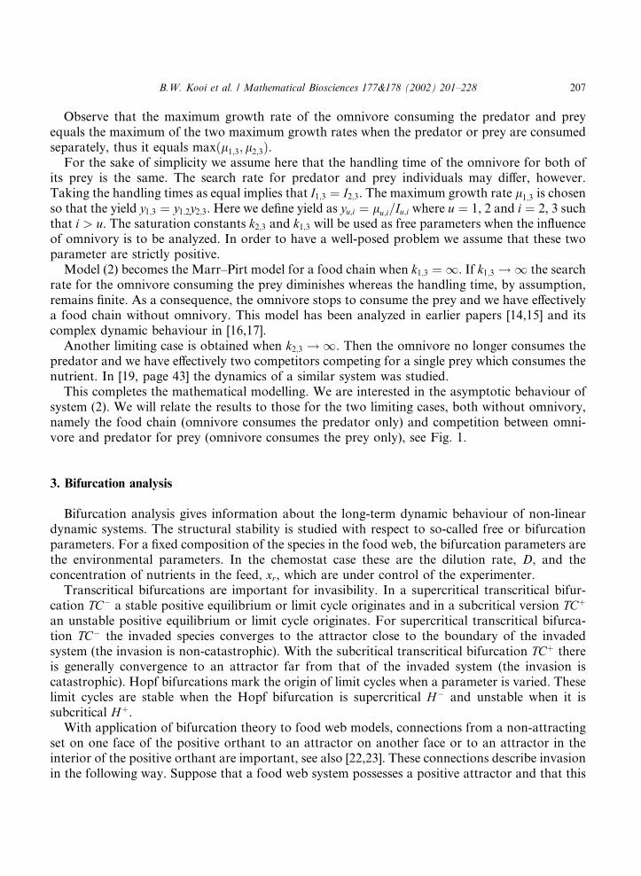
Observe that the maximum growth rate of the omnivore consuming the predator and preyequals the maximum of the two maximum growth rates when the predator or prey are consumedseparately, thus it equals maxðl1;3; l2;3Þ.

For the sake of simplicity we assume here that the handling time of the omnivore for both ofits prey is the same. The search rate for predator and prey individuals may differ, however.Taking the handling times as equal implies that I1;3 ¼ I2;3. The maximum growth rate l1;3 is chosenso that the yield y1;3 ¼ y1;2y2;3. Here we define yield as yu;i ¼ lu;i=Iu;i where u ¼ 1, 2 and i ¼ 2, 3 suchthat i > u. The saturation constants k2;3 and k1;3 will be used as free parameters when the influenceof omnivory is to be analyzed. In order to have a well-posed problem we assume that these twoparameter are strictly positive.

Model (2) becomes the Marr–Pirt model for a food chain when k1;3 ¼ 1. If k1;3 ! 1 the searchrate for the omnivore consuming the prey diminishes whereas the handling time, by assumption,remains finite. As a consequence, the omnivore stops to consume the prey and we have effectivelya food chain without omnivory. This model has been analyzed in earlier papers [14,15] and itscomplex dynamic behaviour in [16,17].

Another limiting case is obtained when k2;3 ! 1. Then the omnivore no longer consumes thepredator and we have effectively two competitors competing for a single prey which consumes thenutrient. In [19, page 43] the dynamics of a similar system was studied.

This completes the mathematical modelling. We are interested in the asymptotic behaviour ofsystem (2). We will relate the results to those for the two limiting cases, both without omnivory,namely the food chain (omnivore consumes the predator only) and competition between omni-vore and predator for prey (omnivore consumes the prey only), see Fig. 1.

3. Bifurcation analysis

Bifurcation analysis gives information about the long-term dynamic behaviour of non-lineardynamic systems. The structural stability is studied with respect to so-called free or bifurcationparameters. For a fixed composition of the species in the food web, the bifurcation parameters arethe environmental parameters. In the chemostat case these are the dilution rate, D, and theconcentration of nutrients in the feed, xr, which are under control of the experimenter.

Transcritical bifurcations are important for invasibility. In a supercritical transcritical bifur-cation TC� a stable positive equilibrium or limit cycle originates and in a subcritical version TCþ

an unstable positive equilibrium or limit cycle originates. For supercritical transcritical bifurca-tion TC� the invaded species converges to the attractor close to the boundary of the invadedsystem (the invasion is non-catastrophic). With the subcritical transcritical bifurcation TCþ thereis generally convergence to an attractor far from that of the invaded system (the invasion iscatastrophic). Hopf bifurcations mark the origin of limit cycles when a parameter is varied. Theselimit cycles are stable when the Hopf bifurcation is supercritical H� and unstable when it issubcritical Hþ.

With application of bifurcation theory to food web models, connections from a non-attractingset on one face of the positive orthant to an attractor on another face or to an attractor in theinterior of the positive orthant are important, see also [22,23]. These connections describe invasionin the following way. Suppose that a food web system possesses a positive attractor and that this


attractor is approached, called the non-invaded system and state respectively. Now a species,called the invader, is introduced. The dimension of the system including the invader and its state-space is one greater than that of the non-invaded system. When the non-invaded state is non-attracting with respect to this extended system, the introduced species can invade successfully. Thesolution of the invaded system will converge to an interior or another boundary attractor in whichcase another species is doomed to die out. Similarly as in [17] for the food chain case, it can beshown that all orbits starting in the interior of the orthant are bounded also when omnivory isincluded.

With multiple attractors a separatrix, which is formed by the stable manifold of an unstableinvariant set, must exist. Each attractor has a domain of attraction and the invaded systemconverges to the attractor in whose domain of attraction the non-invaded state lies. When thenon-invaded state changes the domain of attraction following upon a variation of a free pa-rameter, we have a global bifurcation. At the bifurcation point there is a heteroclinic connectionfrom the non-invaded state to the unstable invariant set which supports the separatrix. An as-

Table 2

List of all bifurcations, codimension-one curves and codimension-two points

Bifurcation Description

Codim-1 curves

TC�e;i Transcritical bifurcation: invasion through boundary equilibrium by prey (i ¼ 1), predator (i ¼ 2) or

omnivore (i ¼ 3), origin of stable (supercritical, � ¼ �) or unstable (subcritical, � ¼ þ) interior

equilibrium

TC�e;32 Transcritical bifurcation: invasion through boundary equilibrium by predator 2 in nutrient–prey–

omnivore system, origin of stable interior equilibrium

TC�c;3 Transcritical bifurcation: invasion through boundary limit cycle omnivore invasion in nutrient–prey–

predator system, origin of stable (supercritical, � ¼ �) or unstable (subcritical, � ¼ þ) interior limit

cycle

TC�c;32 Transcritical bifurcation: invasion through boundary limit cycle by predator 2 in nutrient–prey–

omnivore system, origin of stable interior limit cycle

H�2 Supercritical Hopf bifurcation for nutrient–prey–predator system food web becomes unstable and

origin of stable limit cycle

H�13 Supercritical Hopf bifurcation for nutrient–prey–omnivore food web becomes unstable and origin of

stable limit cycle

H�3 Hopf bifurcation for nutrient–prey–predator–omnivore system food web becomes unstable and origin

of stable (supercritical, � ¼ �) or unstable (subcritical, � ¼ þ) limit cycle

Fi Flip bifurcation: period doubling of limit cycle, origin of stable period-2 limit cycle

Ze;2 Coexistence of the prey and predator

G6¼e;c Global bifurcation of a heteroclinic connection between equilibrium with x2 ¼ 0 and saddle limit cycle

Codim-2 points

N Intersection of TCe;2, TCe;13

M1 Intersection of H�2 , TCe;3, TCc;3

M2 Intersection of TCe;3, Te;3M3 Intersection of TCc;3, Tc;3M4 Intersection of H�

13, TCe;32, TCc;32

P1, P2 Intersection of TCe;32, F13, F3

G Intersection of TCc;3, TCe;13, G6¼e;c


sembly sequence from bare space to a field inhabited by all species, is formed when species areintroduced one at a time, and after the invaded system approached an attractor. This goes on untilthe end-point is resistant to further invasion. Note that the connections to the end-point are notheteroclinic connections because it terminates at an attractor, but in previous stages of the se-quence they are.

Table 2 lists the important bifurcation curves and points. The local bifurcation curves arecalculated with LOCBIF: [24,25] and AUTO: [26]. The global bifurcation is continued with thenumerical technique described in the Appendix A.

The values of the vital parameters of the populations and of those describing the populationinteraction are given in Table 4 and are based on measured data given in [12] for a microbial foodchain.

In the following sections we start in Section 3.1 with the description of dynamic behaviour ofthe predator–omnivore competition model and continue in Section 3.2 with the numerical bi-furcation analysis of a model with the generalist omnivore where it consumes the predator andprey proportional to their biomass.

3.1. Predator–omnivore competition, k1;3 ¼ 1 and k2;3 ¼ 1

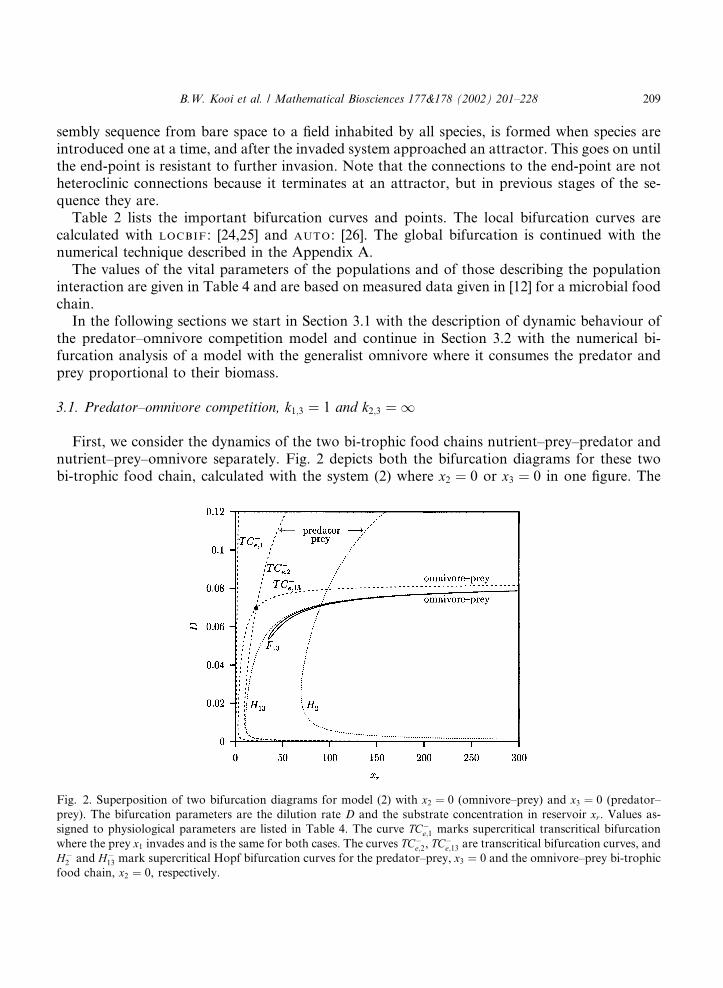
First, we consider the dynamics of the two bi-trophic food chains nutrient–prey–predator andnutrient–prey–omnivore separately. Fig. 2 depicts both the bifurcation diagrams for these twobi-trophic food chain, calculated with the system (2) where x2 ¼ 0 or x3 ¼ 0 in one figure. The

Fig. 2. Superposition of two bifurcation diagrams for model (2) with x2 ¼ 0 (omnivore–prey) and x3 ¼ 0 (predator–

prey). The bifurcation parameters are the dilution rate D and the substrate concentration in reservoir xr. Values as-

signed to physiological parameters are listed in Table 4. The curve TC�e;1 marks supercritical transcritical bifurcation

where the prey x1 invades and is the same for both cases. The curves TC�e;2, TC

�e;13 are transcritical bifurcation curves, and

H�2 and H�

13 mark supercritical Hopf bifurcation curves for the predator–prey, x3 ¼ 0 and the omnivore–prey bi-trophic

food chain, x2 ¼ 0, respectively.


parameter values are given in Table 1, except k1;3 ¼ 1. The curves TC�e;1, TC�

e;2 and TC�e;13 are

transcritical bifurcation curves and H�2 and H�

13 mark supercritical Hopf bifurcation curves. Withfixed dilution rate D (for example D ¼ 0:02) and increasing xr, that is enrichment, the sequence ofattractors for the nutrient–prey–predator system is

E0 !TC�

e;1E1 !

TC�e;2

E2!H�

2L2: ð3Þ

We use the notation introduced in Table 3. The bifurcation curves TC�e;1, TC

�e;2 and H�

2 are the onlybifurcation curves found in the region of the bifurcation diagram we investigate. This is an ex-ample of a simple sequence. First, when no species is present there is the stable equilibrium E0,x0 ¼ xr. When the prey is introduced at a higher xr level, this equilibrium is unstable in R2

þ andthere is convergence to the stable equilibrium E1 2 intR2

þ. When the predator is introduced and xrin increased further there is a stable equilibrium E2 2 intR3

þ. When the xr in increased even furtherthe system approaches a stable limit cycle L2 2 intR3

þ and this is associated with the ‘paradox ofenrichment’.

For the nutrient–prey–omnivore system this sequence of attractors is

E0 !TC�

e;1E1 !

TC�e;13

E13!H�

13L13: ð4Þ

For this nutrient–prey–omnivore food chain the curve F13 marks a flip bifurcation. Calculationsrevealed that this flip bifurcation forms the starting point of a cascade of period doubling bi-furcations leading to chaos. Notice that without maintenance (mi ¼ 0 or Di ¼ D for i ¼ 1; 2; 3)chaos is impossible because the system can be reduced to a two dimensional system when as-ymptotic behaviour is concerned and the conservation principle described in [19] is used.

Now, the predator and omnivore compete for the prey in the chemostat. In this case, theomnivore is a specialist where it consumes the prey but not the predator, that is k2;3 ! 1. Theequations read

dx0

dt¼ ðxr � x0ÞD� I0;1f0;1x1; ð5aÞ

dx1

dt¼ l0;1f0;1

�� D1

�x1 � I1;2f1;2x2 � I1;3f1;3x3; ð5bÞ

dx2

dt¼ l1;2f1;2

�� D2

�x2; ð5cÞ

Table 3

Equilibria and limit cycles of the nutrient–prey–predator–omnivore food web (Fig. 1). The bar denotes the equilibrium

value of the state variable and the tilde their periodic fluctuations in the limit cycles case

Equilibrium Limit cycle Complex

Nutrient E0 ¼ ðx0; 0; 0; 0ÞNutrient–prey E1 ¼ ðx0; x1; 0; 0ÞNutrient–prey–predator E2 ¼ ðx0; x1; x2; 0Þ L2 ¼ ðexx0; exx1; exx2; 0ÞNutrient–prey–omnivore E13 ¼ ðx0; x1; 0; x3Þ L13 ¼ ðexx0; exx1; 0; exx3Þ C13

Nutrient–prey–predator–omnivore E3 ¼ ðx0; x1; x2; x3Þ L3 ¼ ðexx0; exx1; exx2; exx3Þ C3


dx3

dt¼ l1;3f1;3

�� D3

�x3; ð5dÞ

where we use the (scaled) Holling type II functional response denoted by fu;i and defined by

fu;i ¼xu

ku;i þ xu: ð6Þ

Let M1;iðx1Þ, for i ¼ 2; 3, denote the actual specific growth rate of population xi consuming theirprey x1 defined as

M1;iðx1Þ ¼ l1;ix1

k1;i þ x1

�� mi

�: ð7Þ

Let the dilution rate denoted by D� be determined by the condition that the growth rate for thetwo competitors is the same. It forms together with the nutrient concentration x�1, where the bardenotes the equilibrium value, the solution of the following two equations:

M�1;2¼

defl1;2

x�1k1;2 þ x�1

� m2 ¼ D�; ð8aÞ

M�1;3¼

defl1;3

x�1k1;3 þ x�1

� m3 ¼ D�: ð8bÞ

With the values given in Table 4 where k1;3 ¼ 1 instead of k1;3 ¼ 10 the critical value for thedilution rate is D� ¼ 0:06953. This implies that the two transcritical curves for the competingpredator and omnivore TC�

e;2 and TC�e;13, respectively, intersect in the point denoted by N where

D ¼ D�.Fig. 3 depicts the two-parameter bifurcation diagram where the dilution rate D and the con-

centration in the feed xr are the free parameters. On the curve Ze;2 both predators can coexistencein equilibrium with the prey. The solution is, however, degenerated that is the solutions of theequilibrium equations form a one-dimensional manifold in the state space fixed by a linear re-lationship between x2 and x3. Between N and M4 the other three eigenvalues have negative realpart for positive biomasses x2 and x3. On the right-hand side of point M4 (also of point M1) twoeigenvalues have negative real parts.

Table 4

Parameter set for bacterium-ciliate models, after [12,13]

Parameter Unit Values

i ¼ 1 i ¼ 2 i ¼ 3

j ¼ 1 j ¼ 1 j ¼ 1 j ¼ 2

li�j;i h�1 0.5 0.2 0.15 0.09

ki�j;i mg dm�3 8 9 10 10

Ii�j;i h�1 1.25 0.33 0.25 0.25

mi h�1 0.025 0.01 0.0075

The values for the maintenance rate coefficients are taken 5% of the maximum growth rate. The ranges for the control

parameters are 0 < D < l0;1 and 0 < xr 6 300 mg dm�3. Notice that we took for the yield y1;3 ¼ l1;3=I1;3 ¼ y1;2y2;3 ¼ 0:36

and consequently we have l1;3 ¼ 0:6l2;3 since we assumed I1;3 ¼ I2;3. The values are for a generalist omnivore.


In [19, page 43] also competition at a higher trophic level is dealt with. However, the growthrates are of the Monod type, that is no maintenance is assumed: mi ¼ 0 or Di ¼ D for all i. It isproven that the two predators x2 and x3 could survive on a common prey x1 and conditions for theparameters are derived. Furthermore it is mentioned that chaotic behaviour was observed.

Fig. 3 shows the calculated transcritical curves for limit cycles TC�c;3 originating in codim-2 point

M1, and curve TC�c;32 originating in M4. Crossing the TC�

c;3 curve inward into the region between thetwo curves the omnivore can invaded the cycling nutrient–prey–predator system and crossing thecurve TC�

c;32 the predator can invaded the cycling nutrient–prey–omnivore system. In agreementwith the results presented in [19, page 43] there is coexistence of the two predator populations as anon-equilibrium attractor between the curves TC�

c;3 and TC�c;32.

In [17] we discussed the link between invasion and the transcritical bifurcation. The growthrate of the omnivore M1;3 is proportional to its biomass x3 and this implies directly that the in-vasion criterion equals M1;3 > D for equilibrium E2 ¼ ðx0; x1; x2; 0Þ and for a limit cycle L2 ¼ðexx0; exx1;exx2; 0Þ it is T�1

0

R T0

0M1;3ðtÞdt > D where T0 is the period, see [17,19]. When the equal sign

holds, these two criteria are equivalent with the requirement that one eigenvalue equals zero at theequilibrium and one Floquet multiplier has magnitude equal to one at the limit cycle and this fixesthe transcritical bifurcation.

The curve marked by F3 denotes a flip bifurcation. Inside the region bounded by the curve F3 acascade of period doubling leads to chaotic behaviour, but we will not explore this further. Thesituation close to the codim-2 point M4 is more complicated. Fig. 4 shows a detail of the bifur-cation diagram around the codim-2 point M4. In two additional codim-2 points P1 and P2 theflip bifurcation curve F3 intersects the transcritical bifurcation curve TC�

c;32. In these points one

Fig. 3. Bifurcation diagram for model with pure competition between the omnivore and the predator system (5). The

bifurcation parameters are the dilution rate D and the substrate concentration in reservoir xr. Values assigned to

physiological parameters are listed in Table 4 where k1;3 ¼ 1 and k2;3 ¼ 1. The curves TC�e;1, TC�

e;2, TC�e;13, TC�

e;32, TC�e;3 are

transcritical bifurcation curves for equilibria, TC�c;32, TC

�c;3 for limit cycles, and H�

2 and H�13 mark supercritical Hopf

bifurcation curves for the bi-trophic food chains without omnivore, x3 ¼ 0 and predator, x2 ¼ 0, respectively.


Floquet multiplier equals �1 because of the flip bifurcation, F3, and one equals 1 because of thetranscritical bifurcation, TC�

c;32. There are four multiplier for this four dimensional nutrient–prey–predator–omnivore system, and since one multiplier equals always 1 for the motion along theorbit, there is one multiplier not on the unit cycle in the complex plane. The magnitude of thismultiplier was less than 1 for the parameter values given in Table 4 where k1;3 ¼ 1. Furthermore,because these points are on the transcritical bifurcation curves TC�

c;32 we have x2 ¼ 0 and thisimplies that points P1 and P2 are also on the flip bifurcation curve F13 for the three dimensionalnutrient–prey–omnivore system.

Fig. 5 explains what happens when the curve between the two points N and M1 is crossed byvarying D. Between N and M4 the curve Ze;2 coincides actually with both bifurcation curves TC�

e;13

and TC�e;3 and between M4 and M1 with the two bifurcation curves H�

3 and TC�e;3. When D > D� in

the neighbourhood of Ze;2 the predator always out-competes the omnivore and there is an stableequilibrium E2, that is x2 > 0 and x3 ¼ 0. No non-equilibrium attractor exist in this region ofthe bifurcation diagram and therefore classical competitive exclusion holds true. For D < D� inthe neighbourhood of Ze;2 between the points N and M4, the omnivore always out-competes thepredator, that is x2 ¼ 0 and x3 > 0. However, just below the Ze;2 curve and between the points M1

and M4, there is coexistence as a non-equilibrium attractor: a limit cycle L3.

3.2. The generalist omnivore, k1;3 ¼ 10, k2;3 ¼ 10

In this section we discuss the bifurcation diagram displayed in Fig. 6 for the whole food webincluding the omnivore which is now a generalist, k1;3 ¼ 10 and k2;3 ¼ 10. Besides the handlingtime by the omnivore, also the search rate is the same for both predator and prey individuals. The

Fig. 4. Detail of Fig. 3. In the codimension-two bifurcation points, Pj, j ¼ 1; 2 the flip bifurcation curves F13 and F3

intersect each other and the transcritical curve TC�c;32.


omnivore preys on the predator and prey in proportion to their biomass density. For the growthrate of the omnivore the two terms are weighted by the maximum growth rates on the predatorl2;3 and prey l1;3 separately.

Fig. 6. Bifurcation diagram for the model with omnivory: system (2). The bifurcation parameters are the dilution rate

D and the substrate concentration in reservoir xr. Values assigned to physiological parameters are listed in Table 4

where k1;3 ¼ 10 and k2;3 ¼ 10. The curves TC�e;1, TC�

e;2, TC�e;32, TC

�e;3 are transcritical bifurcation curves for equilibria, TC�

c;3

for limit cycles and H�2 , H�

13 mark supercritical Hopf bifurcation curves all for the bi-trophic food chains without and

with perturbations of the vital rates. The curve Hþ3 marks a subcritical Hopf bifurcation for the complete food web.

Point G is a codimension two point for a global bifurcation where the global bifurcation curve G6¼e;c originates.

Fig. 5. Detail of Fig. 3 where only the codimension-two bifurcation points and the attractor types defined in Table 3 are

indicated.


The diagram Fig. 6 shows the calculated transcritical curves for equilibria TC�e;3 originating in

codim-2 point M1 and curve TC�e;32 originating in M4 besides the curves already discussed in the

previous subsection.Let the specific growth rate of the predator, M2, be defined as

M2 ¼ l1;2

x1

k1;2 þ x1

� I2;3k2;3

x3

1 þ x1=k1;3 þ x2=k2;3

� m2: ð9Þ

In an equilibrium E13 ¼ ðx0; x1; 0; x3Þ the invasion criterion reads M2 > D where the growth rate iscalculated in the equilibrium. When invasion is via a limit cycle L13 ¼ ðexx0;exx1; 0; exx3Þ the criterionreads T�1

0

R T0

0M2ðtÞdt > D, where T0 is again the period.

Note that the specific growth rate of the invading species, in this case the predator, into thevirgin environment depends on the abundance of its prey, but also on that of the rival, in this casethe omnivore. More prey is advantageous now for two reasons, directly from the first term of theright-hand side of Eq. (9) but also indirectly from the second term, because the omnivore spendsalso time on handling the prey and this diminishes the rate at which it is consumed by the om-nivore.

Similar invasion criteria hold for the invasion of the omnivore in the nutrient–prey–predatorsystem where the specific growth rate of the omnivore M3 is defined as

M3 ¼l1;3=k1;3 x1 þ l2;3=k2;3 x2

1 þ x1=k1;3 þ x2=k2;3

� m3: ð10Þ

In Fig. 7 the omnivore invades the predator–prey system via a limit cycle L2 ¼ ðexx0;exx1;exx2; 0Þ be-cause T�1

0

R T0

0M3ðtÞdt > D where the growth rate M3ðtÞ is integrated along the limit cycle. The

system converges to three different end-points depending on the environmental conditions D and xr.The diagram depicted in Fig. 6 resembles that of a food chain, already shown and discussed in

[15]. Here we discuss only phenomena due to omnivory. In a food chain a species at a highertrophic level can only exist when species at all lower trophic levels exist. This does not hold truefor omnivory, the omnivore at level three can exist without the predator at level two since it canlive on prey only. This gives the ‘new’ transcritical bifurcation curves TC�

13 and TC�32. It is possible

that, for instance, the predator establishes itself while the omnivore is eliminated or the other wayaround. Furthermore, the end-point of the food web depends on the order in which the predatorand the omnivore are introduced.

In Fig. 8 the equilibrium values for the biomass x1, x2 and x3 are displayed for various dilutionrates 0:066D6 0:1 where xr ¼ 300. The long-term extreme values for exx3 are shown where theattracting state is a limit cycle.

The arrows in Fig. 8 indicate a hysteresis loop. Following the positive solid curves in thedirection of the arrow we find stable equilibria at increasing dilution rates. Then suddenlythe system collapses. The downward arrow indicates that the omnivore is doomed to die out. Thesystem becomes a stable oscillating bi-trophic food chain, as indicated by the solid line at x3 ¼ 0,and invasion by the omnivore is impossible. The omnivore can invade the nutrient–prey–predatorsystem when the dilution rate is lowered sufficiently. Following the arrow to the left, the bi-trophiclimit cycle becomes unstable. When a small amount of omnivore is introduced to the system atlower dilution rates, the system evolves to a stable limit cycle of the nutrient–prey–predator–omnivore system in a small range for the dilution rate. For D values below this point, invasion of


the nutrient–prey–predator system is possible. Initially the system cycles in the x3 ¼ 0 subspace.When the omnivore is inoculated the solution approaches an equilibrium where the predator isabsent, similar as in the middle panel of Fig. 7. Hence the omnivore stabilizes the cycling systemand it replaces the predator, a form of competitive exclusion again.

The sharp bend in the equilibrium values of the biomasses found when D is increased again,marks the point above which persistence of all populations is possible. Finally, when the dilutionrate is increased further, the system remains stable until the omnivore gets suddenly washed-outagain.

These phenomena are now explained using the one-parameter bifurcation diagram depicted inFig. 9. We follow the same loop and the transitions are now indicated by the types of bifurcationthat occur. For D values above the subcritical Hopf bifurcation Hþ

3 the omnivore is washed-out.

Fig. 7. Invasion of the omnivore. Time evolution for the biomass densities x1, x2 and x3 are shown. At t ¼ 0 the

omnivore is inoculated at a small value close to the saddle limit cycle L2, and the omnivore invades the system. For

parameters values D ¼ 0:06 and xr ¼ 150 (top) the system converges to the positive stable equilibrium E3 (L2 ! E3), for

D ¼ 0:02 and xr ¼ 150 (middle) to the stable equilibrium E13 where x2 ¼ 0 (L2 ! E13) and D ¼ 0:02 and xr ¼ 300

(bottom) to the stable limit cycle L13 (L2 ! L13).


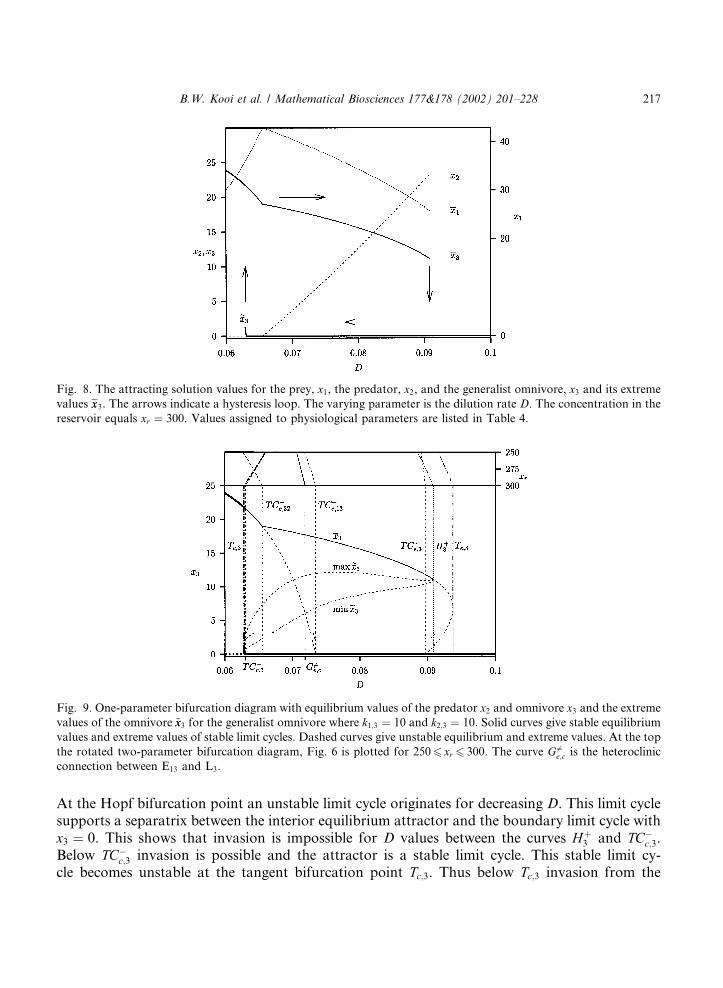
At the Hopf bifurcation point an unstable limit cycle originates for decreasing D. This limit cyclesupports a separatrix between the interior equilibrium attractor and the boundary limit cycle withx3 ¼ 0. This shows that invasion is impossible for D values between the curves Hþ

3 and TC�c;3.

Below TC�c;3 invasion is possible and the attractor is a stable limit cycle. This stable limit cy-

cle becomes unstable at the tangent bifurcation point Tc;3. Thus below Tc;3 invasion from the

Fig. 9. One-parameter bifurcation diagram with equilibrium values of the predator x2 and omnivore x3 and the extreme

values of the omnivore ~xx3 for the generalist omnivore where k1;3 ¼ 10 and k2;3 ¼ 10. Solid curves give stable equilibrium

values and extreme values of stable limit cycles. Dashed curves give unstable equilibrium and extreme values. At the top

the rotated two-parameter bifurcation diagram, Fig. 6 is plotted for 2506 xr 6 300. The curve G 6¼e;c is the heteroclinic

connection between E13 and L3.

Fig. 8. The attracting solution values for the prey, x1, the predator, x2, and the generalist omnivore, x3 and its extreme

values exx3. The arrows indicate a hysteresis loop. The varying parameter is the dilution rate D. The concentration in the

reservoir equals xr ¼ 300. Values assigned to physiological parameters are listed in Table 4.


boundary limit cycle is catastrophic with convergence to the stable equilibrium without predators.Between the two bifurcations Tc;3 and TC�

c;32 a stable limit cycle for the complete food web coexistswith a stable equilibrium where the predator is absent, x2 ¼ 0. The saddle limit cycle in betweenacts again as a separatrix. At the transcritical bifurcation point TC�

c;32 the predator appears andthere is a stable equilibrium for the nutrient–prey–predator–omnivore system for D values abovethis point. This gives the sharp bend in the equilibrium values for the omnivore at that point. Forincreasing D the system remains positive and stable until the catastrophic bifurcation Hþ

3 .The curve TC�

c;13 marks the D value above which the omnivore can invade the nutrient–preysystem. As explained in the next paragraph, since k2;3 ¼ 10, with pure competition of the predatorand omnivore both consuming the prey, the predator wins for all D values.

There must be a global bifurcation for the heteroclinic connection of the boundary saddleequilibrium E1;3 to the interior saddle limit cycle L3 which originates at the subcritical Hopf bi-furcation Hþ

3 . Between the two curves TC�c;3 and TC�

e;13 there are two attractors, the stable equi-librium point E3 and the limit cycle L2 which is also stable because invasion via the omnivore isimpossible for D values between TC�

c;3 and TC�e;13. Since the equilibrium E1;3 is unstable, intro-

Fig. 10. Invasion of the predator near a heteroclinic bifurcation. Time evolution for the biomass densities x1, x2 and x3

are shown. The parameters values are as in Fig. 8. At t ¼ 0 the predator is inoculated at a small value close to the saddle

equilibrium E13 and the predator invades the system. For D ¼ 0:0718 (top) the system converges to the positive stable

equilibrium E3 (E13 ! E3) while for D ¼ 0:07185 (bottom) to the stable limit cycle L2 where x3 ¼ 0 (E13 ! L2). For D ¼0:07183 (middle) the heteroclinic connection between E13 and L3 which supports the separatrix is plotted (E13 ! L3).


duction of the predator leads to invasion, but it is not clear to which attractor the system willevolve. It converges to the attractor in the basin of attraction of which it lies. The separatrixbetween these attractors is the stable manifold of the saddle limit cycle L3. Thus when the saddleequilibrium E1;3 lies on this manifold, the system converges to the unstable limit cycle. When D isbelow the global bifurcation point we are looking for, invasion of the predator via E1;3 leads toconvergence to the interior stable equilibrium point E3 similar to the case at point TC�

c;32 and whenabove that point to the stable limit cycle L2 similar to the case at point TC�

c;13 where the omnivoregoes extinct. In the latter case the invading predator replaces the omnivore and this is just thereverse case when D is smaller than TC�

c;3 where the omnivore replaces the predator. This het-eroclinic connection is indicated by G6¼

e;c in Fig. 9 and marks a global bifurcation. In Fig. 10 thesolutions for three D-values and xr ¼ 300 are shown. In the top panel the dilution rate is slightlysmaller than for G6¼

e;c and the invaded system converges to the interior equilibrium E3, that is thereis a connection from E13 to E3. There is convergence to the boundary limit cycle where x3 # 0 whenD is just above the value for G 6¼

e;c. This is a connection between E13 and L2. The middle panelshows the heteroclinic connection to the interior saddle limit cycle L3. Thus, the curve G 6¼

e;c givesthe additional information to which of the two attractors the system will converge after invasion,while the transcritical bifurcations determine whether or not invasion is possible.

The heteroclinic bifurcation G 6¼e;c originates at point G, shown in two-parameter diagram Fig. 6,

where the heteroclinic connection between E13 en L3 enters the positive orthant through theboundary x3 ¼ 0. Since the hyperplane x3 ¼ 0 is invariant, this means that at point G there mustbe transcritical bifurcations for E13 and L3. It follows that point G is the crossing point betweenTC�

e;13 and TCþc;3. In the Appendix A the algorithm for the calculation of the heteroclinic con-

nection and its continuation in the two-parameter plane is described.

4. Consequences of omnivory

In this section we change the two parameters k1;3 and k2;3 which fix in our approach the strengthof omnivory. We will study invasion of the omnivore in an existing predator–prey system.Consequently the end-points are reached via an unique sequence of connections, depending on theenvironmental conditions D and xr:

ð11Þ

For a number of representative values we present the two-parameter bifurcation diagrams in Figs.11 and 12. In these diagrams the codim-2 points are shown together with the end-points of theassembly where we use the notation introduced in Table 3.


In the diagrams in Figs. 11 and 12 the regions where the end-points are in the interior of R4þ, are

indicated in grey inside the thick dotted lines. The end-points are the positive equilibrium, E3, aperiodic orbit, L3, or a chaotic attractor, C3.

First, we discuss the diagrams depicted in Fig. 11 where both parameters k1;3 and k2;3 werealtered simultaneously. In the first column the saturation parameter k1;3 ¼ 1 and in the secondk1;3 ¼ 10. The other saturation parameter k2;3 has three values k2;3 ¼ 1, 10, 1.

Fig. 11. Bifurcation diagrams where both parameters k1;3 and k2;3 for the omnivore–prey and omnivore–predator

trophic interaction are varied. Left column with k1;3 ¼ 1 < k�1;3, see (13), and right column with k1;3 ¼ 10 > k�1;3, where

k2;3 ¼ 1, k2;3 ¼ 10 and k2;3 ¼ 1 from top to bottom. The gray regions mark coexistence of the three species.


For k1;3 ¼ 1 there is a codim-2 point N but not for k1;3 ¼ 10 independent of the value of k2;3.Therefore, we try to find a condition for D� ¼ 0, where point N is on the horizontal axis withxr ¼ 1. With Eq. (8b) the expression for k1;3 denoted as k�1;3 becomes

Fig. 12. Bifurcation diagrams where the parameter k1;3 for the omnivore–prey trophic interaction is varied: k1;3 ¼ 1, 3,

10, 30, 100, 1 where k2;3 ¼ 10. The gray regions mark coexistence of the three species.


x�1 ¼m2k1;2

l1;2 � m2

and k�1;3 ¼ðl1;3 � m3Þx�1

m3

: ð12Þ

Thus

k�1;3 ¼ðl1;3 � m3Þm2k1;2

ðl1;2 � m2Þm3

: ð13Þ

Hence, for k1;3 > k�1;3, k�1;3 ¼ 7:07143 for the vital parameter values given in Table 4, we haveD� < 0 and competitive exclusion gives that the predator out-competes the omnivore for all di-lution rates. The top-right panel diagram in Fig. 11 illustrates this. The top-left panel is the di-agram Fig. 3 for the competition case. There is coexistence of the predator and omnivore speciesas a non-equilibrium attractor. In the region L3 this non-equilibrium attractor is a period-onelimit cycle but in the region C3 it can be higher periodic or chaotic behaviour. Observe that inthese regions the limit cycles L13 and L2 on the boundary of the positive orthant are both unstable.

The middle-left panel where k1;3 ¼ 1 and k2;3 ¼ 10, the three points N, M1 and M4, are not at onestraight line but they mark now the vertex of a triangle like region. In this small region there ispersistence in a stable equilibrium E3. The middle-right panel next to it is the diagram for thegeneralist omnivore already explained in Section 3.2.

In the diagram in the bottom-left panel where k2;3 ¼ 1 the point M1 moved further upwards andthe point M4 moved to the right, outside the xr-range of the diagram. This increases the regionwith persistence of the three species. In the bottom-right diagram the point M1 moved to a pointwith dilution rate above D ¼ 0:12. Here the region of persistence is very large for rather largedilution rates, however, now in a substantial part, region L3, only as a non-equilibrium attractor.

Comparing the diagrams for k1;3 ¼ 1 with those for k1;3 ¼ 10 depicted in Fig. 11 indicates that itis important whether or no the two transcritical bifurcation curves TC�

e;2 (invasion of the omni-vore, x3 ¼ 0, in the prey–predator bi-trophic food chain, x1 P 0, x2 P 0), and TC�

e;13 (invasion ofthe predator, x2 ¼ 0, x1 P 0, x3 P 0, in the prey–omnivore bi-trophic food chain), for the two bi-trophic food chains intersect in codim-2 point N with positive D�. Observe that in all diagrams thebifurcation curves for the nutrient–prey–predator system are the same. This helps to find thecodim-2 points M1 and N since they lie on these curves. These results show that the position of thepoint M1 depends strongly on the k2;3 value, especially when k1;3 is large. The position of point Ndoes not depend on k2;3 since this point is fixed by the mutual independent interactions betweenthe predator and prey, and omnivore and prey, thus parameters k1;2 and k1;3.

Fig. 12 shows the influence of the parameter k1;3 where in all diagrams k2;3 ¼ 10. In the top-leftdiagram with k1;3 ¼ 1 the omnivore consumes the prey most. There are three codim-2 bifurcationpoints, N, M1 and M4. The region of coexistence E3 is an attracting equilibrium that is enclosed bythe three bifurcation curves which connect these points. As in the competition case, there is non-equilibrium coexistence in the region L3.

With k1;3 ¼ 3 there are only two points N, M1 while point M4 lies outside the diagram with largexr value. Non-equilibrium coexistence occurs in a very small part of the diagram in the neigh-bourhood of point M1. In the regions E13 and L13 the nutrient–prey–predator food chain has astable limit cycle, L2, but the omnivore is able to invade and when it approaches the equilibriumE13 or limit cycle L13 the predator is replaced by the omnivore, see Fig. 7 (middle, bottom). Thearea of the region with equilibrium coexistence is larger than with k1;3 ¼ 1.


With k1;3 ¼ 10, the D-value for the bifurcation point N is negative, that is, point N does notexist. In this diagram another codim-2 point appears, M3. Close to that point, stable limit cyclesfor the whole food web occur, but the region where this happens is small, see also Fig. 9.

With k1;3 ¼ 30 the region E3 is rather large but the omnivore out-competes the predator in still arather large part, region E13 of the diagram. With k1;3 ¼ 100 the region where the omnivore andprey coexist is small. However, besides an interior equilibrium in region E3, there is also non-equilibrium coexistence in the regions L3 and C3. With k1;3 ¼ 1, the food chain case, the om-nivore preys only on the predator. The region with non-equilibrium coexistence increased withrespect to the k1;3 ¼ 100 case.

5. Discussion

In [27,28] a nutrient–two-prey–predator food web is analyzed using bifurcation analysis.Generally, in the absence of the predator, one prey can invade and establish itself while the otheris eliminated: this is called competitive exclusion. It was shown that the bifurcation point wherethe two transcritical curves intersect is an important point in the bifurcation diagram for the foodweb. Here we have a similar situation. The position of the codim-2 bifurcation point N dependsonly on the parameters that determine the trophic interaction between the predator–prey andomnivore–prey separately, and consequently not on the mutual predator–omnivore interaction.This is a form of bottom-up control of the community.

For this small-scale food web there are 16 parameters which describe the dynamics of thespecies and their interaction, and 2 control parameters. The two parameters, k1;3 and k2;3 aredirectly related to omnivory. Unfortunately the resulting variations due to the change of these twoparameters depend also on the other 14 parameters.

We mention the effect of the yield y1;3 and maximum growth rate l1;3 which are changes si-multaneously such that in all cases I1;3 ¼ I2;3. In this paper we assume y1;3 ¼ y1;2y2;3 < y2;3 so thatthe prey–omnivore conversion efficiency from prey via the predator into omnivore is the same aswhen prey is directly consumed by the omnivore. For instance, consider the case where the effi-ciencies of the omnivore consuming the predator and the prey are the same, that is y1;3 ¼ y2;3 andconsequently l1;3 ¼ l2;3, while all other parameters are those of the generalist shown in Table 4.Then, the prey–omnivore chain is more efficient than prey–predator–omnivore chain when con-version from prey into omnivore is concerned. We found that even in this case the region withequilibrium coexistence for k1;3 ¼ 100 is slightly larger than for the food chain case k1;3 ¼ 1.When y1;3 > y2;3 and consequently l1;3 > l2;3 the omnivore–prey system dominates especially whenD is small and xr is large, similar to the generalist case (Figs. 11 and 12).

This shows that the sensitivity analysis performed here, does not give a complete picture of theconsequences of omnivory on the dynamics of the food web in general. In this paper the ‘basis’parameter values are based on experimental data for a microbial food web; a carbohydrate-limited substrate, bacterial prey and protozoan predator, while in [2,11] the parameter valuesdetermined by the body sizes and for the metabolic categories (endotherm, vertebrate ectothermand invertebrate) delineated in [29]. Thus, different consequences of omnivory are to be expected.

In [11] the parameter x is referred to as the strength of omnivory, suggesting that it is a measurefor omnivory. However, the calculated diagrams given in [11] depend also on their second


parameter, k1;3x. The fact that some features of the bifurcation diagram are best described by thetwo parameters k1;3 and k2;3, for instance the existence of point N, motivate us to use these twoparameters as a measure for omnivory.

The end-point, the established community, depends on the order in which the predator andomnivore are introduced into the nutrient–prey system in stable equilibrium. We study the dy-namics of the bounded system (2) in the positive orthant R4

þ. Persistence means that the attractoris in the interior of this orthant. With omnivory multiple attractors coexist with possibly at-tractors on the two boundaries of the positive orthant R4

þ. These are the invariant subspaceswhere x2 ¼ 0 and x3 ¼ 0. Invasion is possible when the invariant set in such an invariant subspaceis only attracting in the positive orthant R3

þ associated with the non-invaded system, that is wherethe invader is not taken into account, but non-attracting in the orthant R4

þ associated with theinvaded system, that is where the invader is taken into account even when its biomass is zero onthe boundary bdR4

þ. Different non-trivial situations can occur with invasion of the predator oromnivore:

• Two boundary invariant sets in the subspaces x2 ¼ 0, E13 or L13, and x3 ¼ 0, L2, respectively.One invariant set is unstable and the other stable. This gives replacement of the resident speciesby the invader, L2 ! E13, Fig. 7 (middle) or L2 ! L13, Fig. 7 (bottom).

• Three invariant sets. Two are on the boundary of the orthant in the subspaces x2 ¼ 0, E13, andx3 ¼ 0, L2, respectively and both are unstable. The third is the stable interior invariant set, E3,L3 or C3. When invasion occurs via both boundary invariant sets the system converges to theinterior attractor, E13 ! E3, Fig. 10 (top) and L2 ! E3, Fig. 7 (top).

• Four invariant sets. Two are on the boundary of the orthant in the subspaces x2 ¼ 0 and x3 ¼ 0,respectively, at least one is stable in this case L2 is stable and E13 is unstable. Two are in theinterior, one unstable L3 and one stable E3, L3 or C3. The stable manifold of the unstable limitcycle L3 is the separatrix between L2 and E3, see Fig. 9. When invasion occurs the system con-verges to the interior attractor E13 ! E3, Fig. 10 (top) or to the other boundary attractorE13 ! L2, Fig. 10 (bottom).

With the assumption that the predator is introduced first, the sequence as well as the end-pointare unique.

Other type of heteroclinic connections in low dimensional ecological systems are investigated inthe literature. Heteroclinic cycles in related three species food web models were investigated in[22,23]. For the three species food chain case (k1;3 ¼ 1), a heteroclinic connection between theinterior saddle equilibrium and the saddle limit cycle is in [30] related to a complicated shape ofthe domain of attraction of an interior stable limit cycle or chaotic attractor.

6. Conclusions

The influence of omnivory was investigated using bifurcation analysis of our model at variablefeeding behaviours of the omnivore. Two limiting cases where the omnivore acts as a specialist,competition and a food chain, figured as starting points. Competition was analyzed by consid-ering the two resource–prey–competitor systems separately. In the analysis of these bi-trophic


food chains we encountered chaos for plausible parameter values. This innovative result will bedealt with in a forthcoming paper.

In terms of non-linear dynamic system theory, an assembly sequence is formed by a series ofconnections between equilibria or limit cycles. These are connections between saddle equilibria orlimit cycles at the boundary of the positive orthant, except when there is convergence to a positiveand stable equilibria or limit cycle where all species persist at the invasible resistant end-point.

For the competition case we derived criteria for coexistence of the omnivore and predator.When this condition is met, survival of the two populations on the common prey is possible, onlyas a non-equilibrium attractor. This occurs at rather high dilution rates and moderate nutrientconcentrations in the supply. The generalist omnivore can coexist in equilibrium with the otherspecies in a relatively large part of the diagram. Further reduction of the predation pressure by theomnivore on the prey gives first a larger region but then it declines somewhat until no preyis consumed by the omnivore as in the food chain. Hence, a weak trophic strength between theomnivore and the prey is advantageous. This is partly in agreement with work by McCann et al.[2] where they suggest that weak interactions are essential for community persistence.

The key results are:

• With a mass balance formulation where nutrients are modelled explicitly, a predator–prey sys-tem in the chemostat can show chaotic behaviour for plausible parameter values.

• When the omnivore and the predator are competitors for the common prey, coexistence occursonly as a non-equilibrium attractor.

• A heteroclinic connection from a saddle equilibrium to a saddle limit cycle separates regionsin the bifurcation diagram with different attractors to which the system evolves after invasion.

• The results for a microbial food web in the chemostat indicate that a weak trophic strengthbetween the omnivore and the prey is advantageous.

• Generally, for the vital parameter chosen here, the omnivore–prey system dominates for lowdilution rates and high nutrient inflow rates, the predator–prey system for high dilution ratesand low nutrient inflow rates, while the three species coexist for moderate values.

We consider only invasion of the omnivore in the existing prey–predator system and studyomnivory by variation of the saturation constants of the multi-species functional response, as usedin the description of the trophic interactions between the omnivore and its prey. We recall that allresults with respect to the role of omnivory depend also on the vital parameters, as given in Table 4,which were kept constant. Hence, general statements about the role of omnivory are problematic.We mention the following example. With y1;3 6 y2;3 we found that the region with equilibriumcoexistence for k1;3 ¼ 100 is slightly larger than for the food chain case k1;3 ¼ 1. However, wheny1;3 > y2;3 and consequently l1;3 > l2;3, since we assume I1;3 ¼ I2;3, that is the omnivore assimilatesthe prey more efficient than the predator, equilibrium coexistence with k1;3 ¼ 100 occurs in asmaller region of the two-parameter diagram than for the food chain case k1;3 ¼ 1 instead ofslightly larger. As a result a weak trophic strength between the omnivore and the prey is not ad-vantageous when y1;3 > y2;3.

Application of numerical bifurcation analysis is feasible in a similar context for interactionsin food chains studied in [2,31,32]. This is a next step towards the analysis of natural, and morecomplicated, food webs. The variety of the dynamic behaviours we encountered indicates that


the complete analysis of large-scale or even intermediate-scale food webs on a routine basis ispractically not feasible. When the focus is on applications, for instance conservation and man-agement problems of natural communities where the range of parameter values involved is small,the approach proposed in this paper might prove beneficial.

Acknowledgements

The authors would like to thank Cor Zonneveld for valuable comments and suggestions on thiswork.

Appendix A. Calculation of the heteroclinic connection

In the generalist case we found a global bifurcation denoted by G6¼e;c depicted in Fig. 6. In

this appendix the algorithm is given to calculate the heteroclinic connecting orbits. We use aboundary-value method described in [15,25,33–36]. The heteroclinic problem is truncated into afinite time interval and certain boundary conditions at the end points of that interval are imposed.Suitable boundary conditions are obtained by using linear approximations near the equilibriumpoint E13 and the limit cycle L2.

The continuation of the codim-1 bifurcation curve G6¼e;c in the two-parameter diagram is

computed by solving simultaneously 21 scalar equations for 22 scalar variables.Nine equations are associated with the linear approximations near the equilibrium point E13.

Eqs. (2a)–(2d) with zero right-hand side fix the equilibrium point x. If the system is described bydz=dt ¼ fðzÞ where f : R4

þ ! R4þ (the system is autonomous, hence there is no explicit dependency

on time t), then the equilibrium is determined by the four equations

fðxÞ ¼ 0: ðA:1ÞFive equations fix the normalized eigenvector p 2 R4 and the positive eigenvalue k of the Jacobianmatrix J evaluated at x. This eigenvalue k is just the invasion criterion for invasion of the pre-dator. The equations read

Jp ¼ kp; ðA:2Þ

hp; pi ¼ 1; ðA:3Þwhere hr; si ¼ rTs is the standard scalar product in R4.

Further nine equations are associated with the linear approximations near the limit cycle L3.Let the flow /ðt; xÞ, / : R� R4

þ ! R4þ, denote a solution of system (2a)–(2d) so that /ð0; xÞ ¼ x.

The cross-section R is defined by

R ¼ x 2 R4þ :

l1;3 � D3

k1;3

x1

þ

l2;3 � D3

k2;3

x2 ¼ D3

:

Then the Poincar�ee map P : R ! R is defined for a point z 2 R by P ðzÞ ¼ /ðs; zÞ, where s ¼ sðzÞ isthe time taken for the orbit /ðt; zÞ to first return to R.

The next five equations determine the fixed point y of the Poincar�ee map of the limit cycle L3

defined in R


y ¼ P ðyÞ; ðA:4Þ

y 2 R: ðA:5ÞEq. (A.5) is the phase condition. On the saddle limit cycle we have T0 ¼ sðyÞ. The monodromymatrix associated with the saddle limit cycle L3 [25] is denoted by M. The following four equationsfix the normalized adjoint eigenvector q 2 R4 and one equation the eigenvalue of M denoted by q,being the single multiplier of the Poincar�ee map with magnitude greater than 1.

MTq ¼ qq; ðA:6Þ

hq; qi ¼ 1: ðA:7ÞThe remaining two equations are associated with the boundary-value problem. The truncated

heteroclinic orbit starts at a fixed distance from the point E13 ¼ x on the linear approximationT uðxÞ, of the unstable manifold W uðxÞ fixed by the eigenvector corresponding to the positiveeigenvalue of the Jacobian evaluated at x. Then the set of coupled ODEs (2) which describe thedynamic system, is solve numerically using a Runge–Kutta method for a fixed time period Th

which acts as a free parameter during the continuation process. The two equations

h/ðTh;xþ epÞ � y; qi ¼ 0; ðA:8Þ

/ðTh; xþ epÞ 2 R; ðA:9Þfix the truncated heteroclinic orbit, where e � 1 is a small scalar. Eq. (A.8) ensures that the vectorfrom the fixed point on the limit cycle y 2 R to the endpoint /ðTh;xþ epÞ 2 R, is perpendicular tothe adjoint eigenvector q of the monodromy matrix M corresponding to the multiplier, q, withmagnitude greater than one. The Fredholm alternative [25] gives that the end point is on the linearapproximation T sðyÞ of the stable manifold W sðyÞ of the saddle limit cycle L3 at point y.

The 22 variables: D, xr, x, p, k, y, q, q, T0, Th and the 21 equations: (A.1)–(A.9) determine thecurve G 6¼

e;c in Fig. 6. The continuation of this global bifurcation G 6¼e;c was done by means of a

predictor-corrector continuation method with step-size control [25,37,38]. The initial data for thecontinuation procedure were obtained as follows. With xr ¼ 300 the dilution rate D was changedsmoothly and system (2) was solved numerically starting close to the saddle point E13 ¼ x on thelinear approximation of the unstable manifold. The point where the asymptotic behaviour changedsuddenly (convergence to E3 instead of L13 see Fig. 10) was chosen to start the continuationprocess.

References

[1] A.J. Weatherby, P.H. Warren, Coexistence and collapes: an experimental investigation of the persistent

communities of a protist species pool, J. Animal Ecol. 67 (1998) 554.

[2] K. McCann, A. Hastings, G.R. Huxel, Weak trophic interactions and the balance of nature, Nature 395 (1998) 794.

[3] R.M. May, Stability and Complexity in Model Ecosystems, Princeton University, New Haven, NJ, 1973.

[4] R. Law, R.D. Morton, Permanence and the assembly of ecological communities, Ecology 77 (1996) 762.

[5] S. Diehl, M. Feißel, Effects of enrichment on three-level food chain with omnivory, Am. Natural. 155 (2000) 200.

[6] M.L. Rosenzweig, R.H. MacArthur, Graphical representation and stability conditions of predator–prey inter-

actions, Am. Natur. 97 (1963) 209.


[7] A. Hastings, T. Powell, Chaos in a three-species food chain, Ecology 72 (1991) 896.

[8] Y.A. Kuznetsov, S. Rinaldi, Remarks on food chain dynamics, Math. Biosci. 124 (1996) 1.

[9] O. De Feo, S. Rinaldi, Yield and dynamics of tritrophic food chains, Am. Natural. 150 (1997) 328.

[10] M.P. Boer, B.W. Kooi, S.A.L.M. Kooijman, Homoclinic and heteroclinic orbits in a tri-trophic food chain,

J. Math. Biol. 39 (1999) 19.

[11] K. McCann, A. Hastings, Re-evaluating the omnivory–stability relationship in food webs, Proc. R. Soc. London

(B) 264 (1997) 1249.

[12] A. Cunningham, R.M. Nisbet, Transients and oscillations in continuous culture, in: M.J. Bazin (Ed.), Mathematics

in Microbiology, Academic Press, London, 1983, p. 77.

[13] R.M. Nisbet, A. Cunningham, W.S.C. Gurney, Endogenous metabolism and the stability of microbial prey–

predator systems, Biotechnol. Bioeng. 25 (1983) 301.

[14] B.W. Kooi, M.P. Boer, S.A.L.M. Kooijman, Complex dynamic behaviour of autonomous microbial food chains,

J. Math. Biol. 36 (1997) 24.

[15] B.W. Kooi, M.P. Boer, S.A.L.M. Kooijman, Consequences of population models on the dynamics of food chains,

Math. Biosci. 153 (1998) 99.

[16] M.P. Boer, B.W. Kooi, S.A.L.M. Kooijman, Food chain dynamics in the chemostat, Math. Biosci. 150 (1998) 43.

[17] B.W. Kooi, M.P. Boer, S.A.L.M. Kooijman, Resistance of a food chain to invasion by a top predator, Math.

Biosci. 157 (1999) 217.

[18] A. Gragnani, O. De Feo, S. Rinaldi, Food chains in the chemostat: relationships between mean yield and complex

dynamics, Bull. Math. Biol. 60 (1998) 703.

[19] H.L. Smith, P. Waltman, The Theory of the Chemostat, Cambridge University, Cambridge, 1994.

[20] R.D. Morton, R. Law, S.L. Pimm, J.A. Drake, On models for assembling ecological communities, Oikos 75 (1996)

493.

[21] M.J.W. Cock, Assessment of preference, J. Animal Ecol. 47 (1978) 805.

[22] A.D. Bazykin, Non-linear dynamics of interacting populations, World Scientific, Singapore, 1998.

[23] J. Hofbauer, K. Sigmund, Evolutionary Games and Population Dynamics, Cambridge University, Cambridge,

1998.

[24] A.I. Khibnik, Y.A. Kuznetsov, V.V. Levitin, E.V. Nikolaev, Continuation techniques and interactive software for

bifurcation analysis of ODEs and iterated maps, Physica D 62 (1993) 360.

[25] Y.A. Kuznetsov, Elements of Applied Bifurcation Theory, Springer, New York, 1998.

[26] E.J. Doedel, A.R. Champneys, T.F. Fairgrieve, Y.A. Kuznetsov, B. Sandstede, X. Wang, Auto 97: continuation and

bifurcation software for ordinary differential equations, Tech. rep., Concordia University, Montreal, Canada, 1997.

[27] B.W. Kooi, S.A.L.M. Kooijman, Invading species can stabilize simple trophic systems, Ecol. Modelling 133 (2000)

57.

[28] D.V. Vayenas, S. Pavlou, Chaotic dynamics of a food web in a chemostat, Math. Biosci. 162 (1999) 69.

[29] P. Yodzis, S. Innes, Body size consumer-resource dynamics, Am. Natural. 139 (1992) 1151.

[30] M.P. Boer, B.W. Kooi, S.A.L.M. Kooijman, Multiple attractors and boundary crises in a tri-trophic food chain,

Math. Biosci. 169 (2001) 109.

[31] D.M. Post, M.E. Conners, D. Goldberg, Prey preference by a top predator and the stability of linked food chains,

Ecology 81 (2000) 8.

[32] T.G. Sazykina, V. Alekseev, A.I. Kryshev, The self-organization of trophic structure in ecosystem models: the

succession phenomena, trigger regimes and hysteresis, Ecol. Modelling 133 (2000) 83.

[33] W.-J. Beyn, The numerical computation of connecting orbits in dynamical systems, IMA J. Num. Anal. 9 (1990) 379.

[34] A.R. Champneys, Y.A. Kuznetsov, B. Sandstede, A numerical toolbox for homoclinic bifurcation analysis, Int. J.

Bifurcation Chaos 6 (1996) 867.

[35] A.R. Champneys, G.J. Lord, Computation of homoclinic solutions to periodic orbits in a reduced water-wave

problem, Physica D 102 (1997) 101.

[36] W.-J. Beyn, J.-M. Kleinkauf, The numerical computation of homoclinic orbits for maps, SIAM J. Numer. Anal. 34

(1997) 1207.

[37] E.L. Allgower, K. Georg, Numerical Continuation Methods, Springer, New York, 1990.

[38] T.S. Parker, L.O. Chua, Practical Numerical Algorithms for Chaotic Systems, Springer, New York, 1989.


Documents

Numerical bifurcation analysis of a tri-trophic food web with omnivory