Trophic Interactions, Community Organization, and the Kluane Ecosystem

A. R. E. SINCLAIR & CHARLES j. KREBS

3

The conservation of biodiversity depends on functioning natural ecosystems and com­munities. There are various scientific reasons for conserving natural ecosystems. One

is that we need to retain representative portions of the natural world as base line controls for human impacts elsewhere. Another is that we need to preserve species that may later be of benefit to humans. To conserve natural systems, however, we have to understand how disturbances affect natural systems and whether those effects will cause irreversible changes. Alternatively, in human-dominated systems, we need to understand how changes will affect our own livelihood through the stability of the system.

Communities are highly complex, consisting of a large number of species that inter­act with other species. Studies of communities ask two main questions. First, how are they structured? That is, how many levels, such as plants , herbivores, predators, and top predators, are there? Second, how does the ecosystem work? For example, will the sys­tem be affected if we take out one of the species or several of the species? Alternatively, are some species more important to the viability of the community? These questions are relevant to the idea that systems have a large number of species that perform the same function and that there is a large amount of redundancy (Walker 1991). This idea implies that one can afford to lose species without radically altering the integrity and function­ing of the community. Redundancy in the function of species in the community is a nec­essary safety net for that community, and, if we lose that redundancy (i.e., reduce the di­versity of species), then we run the risk of a collapse in the system from some small external perturbation.

These questions are also relevant to systems that have already been subjected to changes such as eutrophication of lakes, fragmentation of forests, acid rain pollution of lakes and forests, introduction of exotic species, and creation of protected areas as islands within human ecosystems. Removal of the lower trophic levels, the plants, will always change a community and result in habitat loss. Nearly all human endeavor affects lower levels and, hence, alters habitats. However, when herbivores or predators are removed from a system the effects are less predictable and depend on which species are affected. Does the removal of species at higher trophic levels change the nature of the whole com­munity? We know from studies of some ecosystems such as the marine intertidal and coastal systems of the Pacific Coast of North America that, when top predators (in this case sea otters) are removed from the system, the system changes radically from one type of community to another and stays that way until the top predators return (Estes et al. 1989, Wootton 1994a). Therefore, in this ecosystem the removal of a predator radically alters the community. Not all communities, however, may react in this way when a predator is removed.

Because communities are complex and contain large numbers of species, we cannot study every component and put it together like a jigsaw puzzle. Indeed, it is likely that the sum of the component parts (the dynamics of individual populations) will not tell us how the combination of species will interact with each other. We must therefore study the whole community as a functioning unit and try to find general rules for how communities work. It is unlikely that simple generalities will be appropriate for such complex systems, and we recognize that in reality communities will have complex structure and dynamics. However, we must start our research with a simple idea and then expand on that as we

26

TROPHIC INTERACTIONS AND COMMUNITY ORGANIZATION 27

learn more from experimentation. In this chapter we discuss trophic-level theory and lay the theoretical groundwork for the experiments described in the rest of this book.

3.1 Trophic-level Theory

3. 7. 7 Community Structure

Community structure has been studied by comparing food webs (i.e., the connections between different species in natural history studies of communities) across the world. Over the past decades several hundred descriptive studies of food webs have been ex­haustively analyzed (Cohen 1978, Pimm 1982, Briand and Cohen 1987, Paine 1988, Menge and Farrell 1989, Schoener 1989, Hall and Raffaelli 1991, Polis 1991, Schoenly et al. 1991). Despite the incomplete data, a number of general patterns in food webs can be seen (Lawton 1989). Ecologists have suggested rules for how many species one might expect, the types of interactions between species, and the number of trophic levels in dif­ferent parts of the world.

The functioning of these communities-their dynamics-has also been studied by comparative methods and by perturbation experiments. These studies have focused on how one trophic level affects another or on the nature of the interactions between species in the community. Interactions between species can be either direct or indirect. Direct in­teractions are those in which there is a physical relationship between species, such as a predator eating its prey or direct interference between competitors. Indirect interactions along a food chain are those that are one step or more removed. Thus, predation is a di­rect interaction, but the effect of the prey population on the vegetation as a consequence of that predation one level above is an indirect interaction. Other indirect interactions in­volve exploitation competition, in which one predator affects the food supply of another predator, apparent competition, in which two prey species share the same predator, and indirect mutualism, in which a predator affects its prey, which in turn affects the compe­tition between another prey and therefore its own predator (Wootton 1994b). Indirect ef­fects can also arise when one species affects the interaction between two other species, sometimes by a change in behavior (Schmitz 1998). Questions asked at this level of gen­erality involve how far perturbations travel as indirect linkages along the food chain. For example, if the main prey for a predator is removed, does the predator switch to a sec­ondary prey, and how does this affect the secondary prey and its own competitors? Alter­natively, if a predator is removed, how does this alter the competition between various prey species?

3. 7.2 Control of Trophic-level Biomass

Bottom-up hypotheses assume that systems are regulated by nutrient flow from below (White 1978, 1984) because plants are essential to the levels above. Comparative studies have suggested that low soil nutrients and low productivity of plants result in fewer trophic levels, that higher productivity of plants results in more trophic levels, and that a gradient of increasing primary productivity (and more levels) can be traced from high to low lati-

28 ECOSYSTEM DYNAMICS OF THE BOREAL FOREST

tudes (Oksanen et al. 1981, T. Oksanen 1990, Abrams 1993). In this view, higher trophic levels have neither a regulating effect nor any influence on productivity or biomass on the levels below them (Hawkins 1992, Hunter and Price 1992, Strong 1992). In African ter­restrial environments the relationship between nutrients, primary productivity, and sec­ondary productivity has been illustrated by Coe et al. (1976), Botkin et al. (1981), Bell (1982), and McNaughton et al. (1989).

Early ideas of top-down effects can be attributed to Hairston et al. (1960) and Slobod­kin et al. (1967), who proposed predator regulation of herbivores. Although their basic premise that green vegetation is available to be eaten was wrong because much of this vegetation is defended, these authors stimulated a number of other ideas. One is the pure top-down hypothesis, which proposes that each trophic level is regulated by the one above with the top predators being self-regulated. This concept was applied to aquatic and ma­rine systems (Menge and Sutherland 1976). Iftop predators, such as fish in a lake, are re­moved, then lower predator levels increase, herbivores decrease, and plants increase in biomass. This "cascade hypothesis" (Carpenter et al. 1985, Carpenter and Kitchell1987, 1988, 1993) recognizes that nutrient availability uniformly raises or lowers these rela­tionships.

Trophic levels could also alternate between top-down and bottom-up regulation (Fretwell1977, 1987, Oksanen et al. 1981, L. Oksanen 1988, 1990). Thus, predators reg­ulate herbivores which cannot, therefore, regulate their own plant food. Plants are then regulated by nutrients. This idea, called the Fretweli-Oksanen hypothesis, has been ap­plied to the wolf-moose-shrub ecosystem on Isle Royale in Lake Superior (McLaren and Peterson 1994) and to vole communities in Scandinavia (Moen et al. 1993).

The Fretwell-Oksanen hypothesis leads to different predictions in ecosystems with dif­ferent nutrient levels (Fretwel11987, Oksanen and Ericson 1987, L. Oksanen 1990, T. Ok­sanen 1990). Low productivity systems such as on the Arctic tundra support only two trophic levels, plants and herbivores, and in these systems herbivores regulate plants. At higher productivity, such as in temperate terrestrial systems, three trophic levels occur, and plants are nutrient limited. In very productive systems, such as estuaries and some lakes, with four levels, top predators are self-regulating and also regulate lower predators, so that herbivores are regulated from below but also regulate vegetation in tum. There­fore, the plant- herbivore link is a two-way interaction. Two generalities appear from this comparison. First, in systems with even numbers of levels (two, four), herbivores regu­late plants and the vegetation is largely herbaceous (grassland, prairie, tundra, etc.). In sys­tems with odd numbers of levels, predators regulate herbivores, and the vegetation, re­leased from severe herbivory, becomes forest or shrub dominated. Second, the number of levels is determined by the productivity of the system through nutrient availability (i.e., ultimately there is a bottom-up influence).

Other models propose that regulatory effects of higher trophic levels depend not so much on productivity as on the level of environmental stress (Menge and Olson 1990), al­though these two features are quite possibly correlated. Predictions, however, differ de­pending on which trophic level is the more susceptible to stress. If consumers (herbivores, predators) are more susceptible to harsh climate, for example, than are plants, then under severe environmental stress consumers will be inhibited and plants will be regulated from below. Under benign conditions herbivores should regulate plants (Menge and Sutherland 1976, Connell 1978). The alternative view is that plant defenses are inhibited by stress,

TROPHIC INTERACTIONS AND COMMUNITY ORGANIZATION 29

such as drought, whereas consumers are less affected. Thus, consumers can regulate plants under stressful conditions (White 1984, Menge and Olsen 1990). The types of stress dif­fer in these two views. The former involves adaptations to harsh environments and is long term, the latter addresses more short-term events. Both concepts are likely to be valid in different circumstances.

In aquatic systems there is evidence that indirect interactions become diluted the far­ther along the food chain they occur. Thus, a combined top-down, bottom-up hypothesis for aquatic systems suggests that biomass is regulated from below by nutrient availabil­ity, but this effect is strongest at the plant level and becomes weaker at progressively higher levels. Equally at the top of the food web, top-down interactions are strong, but these effects weaken with every step down (McQueen et al. 1986, 1989, Pace and Funke 1991). Other mechanisms that reduce the efficiency of predators are interference and ter­ritoriality of predators and refuges for prey. These result in attenuation of indirect effects at lower links in the chain, and so bottom-up effects are seen at lower trophic levels (Power 1984, Arditi and Ginsburg 1989, Arditi et al. 1991, Hanski 1991).

These concepts have all been expressed verbally and hence they are imprecise. When we discuss an effect of one trophic level on another as a result of a perturbation, we need to define what type of effect is being considered. Thus, there are immediate or "instanta­neous" effects when a change in one trophic level affects another. These may be quite dif­ferent from long-term consequences if the change persists and the system settles at some new equilibrium. For example, in the intertidal community on the Pacific Coast of North America, gulls feed on goose barnacles (Pollicepes spp.) and mussels (Mytilus). When gulls were excluded for 2 years from exclosure plots (Wootton 1994a), there was an in­crease in one prey species (Pollicepes) but a decrease in the other (Mytilus) as a result of space competition with Pollicepes. These are long-term results. The short-term result of gull removal, however, would have been an immediate increase in survival of both prey species. Thus, indirect effects can have complex results farther along the food chain and make them difficult to predict (Yodzis 1988, Wootton 1994b).

3.1.3 Case Studies in Mammalian Communities

Long-term studies have thrown some light on trophic-level dynamics. For example, 40 years of monitoring the large-mammal communities in the Serengeti, Tanzania, revealed the complexities of trophic-level interactions (Sinclair 1995, Mduma eta!. 1999). Her­bivorous mammals can be divided into migrants and residents. Migrant species, such as the wildebeest ( Connochaetes taurinus ), are regulated through their food supply of grasses (monocots). Although top predators (lions, hyenas) feed on wildebeest, they are not lim­ited by this food source, but rather are limited by the supply of resident herbivores. In turn, top predators limit the density of resident herbivores as well as lower level predators such as cheetah (Acinonyx jubatus) and wild dogs (Lycaon pictus) (Laurenson 1995). Many of the resident herbivores feed exclusively on herbs (dicots) and determine their composi­tion. Hence, there is a complex series of control pathways. The migrant herbivores are reg­ulated by bottom-up flow from monocots. In contrast, the resident herbivores are regu­lated by top-down flow from the predators. These conclusions were reached through interpreting perturbations in the ecosystem that acted as seminatural experiments.

Yellowstone National Park, USA, is another system in which the mammalian commu-

30 ECOSYSTEM DYNAMICS OF THE BOREAL FOREST

nity has been studied for several decades (e.g., Houston 1982, Keiter and Boyce 1991). This system was previously perturbed by the removal of the top predator, the wolf (Canis

Lupus) a century ago. As in the Serengeti, the dominant migrant herbivore, elk (Cervus

elaphus), is regulated by food supply. Elk, in turn, determine the vegetation composition, both for the monocots and the dicots, including regenerating young trees such as aspen (Merrill et al. 1994, Singer et al. 1994). The recent reintroduction of wolves to the ecosys­tem will test whether this bottom-up control persists in the migrant herbivores or whether top-down control takes over in both migrant and resident mammalian herbivores.

The intertidal communities along the Pacific Coast of North America (Estes eta!. 1989, Estes and Duggins 1995) show top-down control. Top predators such as sea otters (Enhy­

dra lutris) determine the abundance of sea urchins (Strongylocentrus spp.), the dominant herbivores, and hence indirectly determine the macroalgae composition and other mem­bers of the community.

Conclusions from the intertidal system were obtained from controlled experiments. In contrast, trophic dynamics of terrestrial ecosystems have been difficult to study in con­trolled experiments because of the large scale and the long time needed to produce results. However, by using the small mammal community in the boreal forest of the Yukon at Klu­ane, we have been able to generate perturbation experiments to examine the direction of control between trophic levels. These experiments were designed to perturb each trophic level in turn. We approached the problem of predicting the effects of our perturbations in the boreal forest by considering only immediate or instantaneous effects. Then we started from first principles and considered all the possible outcomes from an experimental per­turbation as the effects traveled along the food chain.

3.2 Interactions of Trophic Levels

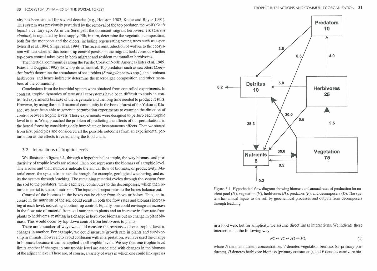
We illustrate in figure 3. 1, through a hypothetical example, the way biomass and pro­ductivity of trophic levels are related. Each box represents the biomass of a trophic level. The arrows and their numbers indicate the annual flow of biomass, or productivity. Ma­terial enters the system from outside through, for example, geological weathering, and ex­its the system through leaching. The remaining material cycles through the system from the soil to the predators, while each level contributes to the decomposers, which then re­turns material to the soil nutrients. The input and output rates to the boxes balance out.

Control of the biomass in the boxes can be either from above or below. Thus, an in­crease in the nutrients of the soil could result in both the flow rates and biomass increas­ing at each level, indicating a bottom-up control. Equally, one could envisage an increase in the flow rate of material from soil nutrients to plants and an increase in flow rate from plants to herbivores, resulting in a change in herbivore biomass but no change in plant bio­mass. This would occur by top-down control from herbivores to plants.

There are a number of ways we could measure the responses of one trophic level to changes in another. For example, we could measure growth rate in plants and survivor­ship in animals. However, to avoid confusion with interpretation, we have used the change in biomass because it can be applied to all trophic levels. We say that one trophic level limits another if changes in one trophic level are associated with changes in the biomass of the adjacent level. There are, of course, a variety of ways in which one could link species

0.2

TROPHIC INTERACTIONS AND COMMUNITY ORGANIZATION 31

Detritus 10

28.3

0.2

5.0

Predators 10

4.0

Herbivores 25

9.5

Vegetation 75

Figure 3.1 Hypothetical flow diagram showing biomass and annual rates of production for nu­trient pool (N), vegetation (V), herbivores (H), predators (P), and decomposers (D). The sys­tem has annual inputs to the soil by geochemical processes and outputs from decomposers through leaching.

in a food web, but for simplicity, we assume direct linear interactions. We indicate these interactions in the following way:

Nt +-+ Vt +-+ Ht +-+ Pt, (1)

where N denotes nutrient concentration, V denotes vegetation biomass (or primary pro­ducers), H denotes herbivore biomass (primary consumers), and P denotes carnivore bio-

32 ECOSYSTEM DYNAMICS OF THE BOREAL FOREST

mass (secondary consumers). The arrows denote trophic-level effects, with a rightward arrow implying that an increase in resource (food) increases the rate of change of biomass of the adjacent consumer level. Similarly, a leftward arrow implies that an increase in con­sumer biomass decreases the rate of change of the adjacent prey biomass. A vertical ar­row implies that a given trophic level has a density-dependent effect on its own rate of growth.

Some of the food web structures one could think of would be biologically implausible. For example, a terminal trophic level that has no negative feedback on its growth would grow infinitely. Accordingly, there must be an intraspecific feedback effect at the end of each plausible chain or else a link between the penultimate and terminal levels. For sim­ilar reasons, it would not be biologically plausible to have arrangements such as the fol­lowing:

(2)

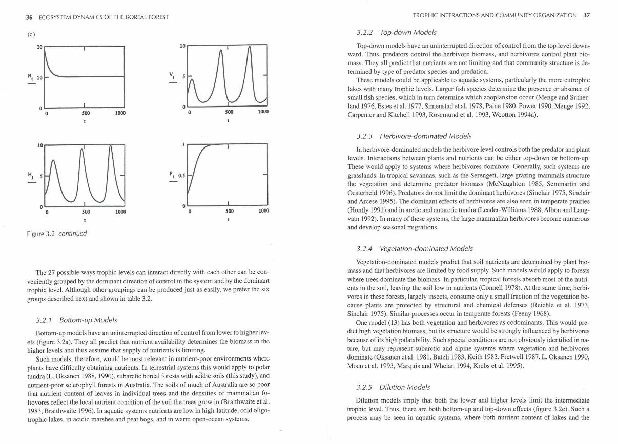
because there would be no negative feedback on the rate of growth in any of the trophic levels and so all would grow exponentially over time. Therefore, we assume that there must be some feedback on each level, and possible competition within the trophic levels (i.e., there is always a vertical arrow at each level implied in our models). The algebraic formulations for instantaneous change at each trophic level are illustrated in table 3.1 for three basic types of bottom-up, top-down and reciprocal control (Sinclair et al. 2000). There are, however, 27 biologically plausible models (table 3.2), all of which have nega­tive feedbacks at every link in the web, either due to self-limited growth or an impact from the next highest level. All models comprise various combinations of the equations in table 3.1 (J. M. Fryxell, personal communication). The majority of the models are highly sta­ble, each level equilibrating monotonically or with a few minor fluctuations. Figure 3.2 illustrates the time dynamics of three of the models. Figure 3.2a shows the stable, pure bottom-up model 1. Figure 3.2b shows the pure reciprocal model 27 with some damped fluctuation. Only three models show more marked fluctuation, and they all involve recip7 rocal interactions between plants and herbivores with predators imposing top-down con­trol (models 7, 20, 22). Figure 3.2c illustrates model20 involving double dilution effects (see table 3.2).

We have assumed in our equations the simplest (linear) density-dependent relation­ships. For illustrative purposes, consider interactions between plants (V) and herbivores (H). A left arrow implies that changes in herbivore density affects the rate of plant bio­mass change, near equilibrium, but not vice versa. Such a situation implies that herbivore growth is limited by something other than food, even though herbivores do consume plants. For example, hares feed on white spruce, and the higher the density of hares, the heavier the browsing impact on the trees. However, hare survival is little affected by spruce biomass. Similarly, a right arrow implies that changes in plant density affect the rate of change of herbivore biomass, near equilibrium, but not vice versa. Biologically this occurs when red squirrels feed on cones, hares eat senescent willow leaves, and carnivores rely on carrion. A double-headed horizontal arrow between plants and herbivores implies that herbivores respond to plant abundance, and plants, in turn, respond to herbivore abun­dance, forming a reciprocal relationship (Caughley 1976). Finally, a density-dependent form of intraspecific competition implies that each trophic level has its own intrinsic limits.

Table 3.1 Minimal algebraic expressions for bottom-up, top-down, and reciprocal interactions between trophic levels.

Bottom-up Interactions

dN - = ro -aooN dt

dV 2 - = a10NV- a11 V dt

Top-down Interactions

dV 2 - = r1 V - a12 VH - a 11 V dt

dH 2 - = r2H- a23 HP- a22H dt

Reciprocal Interactions

dN - = 'O - aooN- aolNV dt

, r, is the per capita rate of increase of trophic level i; a,

1 is the community matrix coefficient for trophic levelj acting

on trophic level i. N = soil nutrient pool, V = plant biomass, H = herbivore biomass, P = predator biomass. All models

use some combination of these equations.

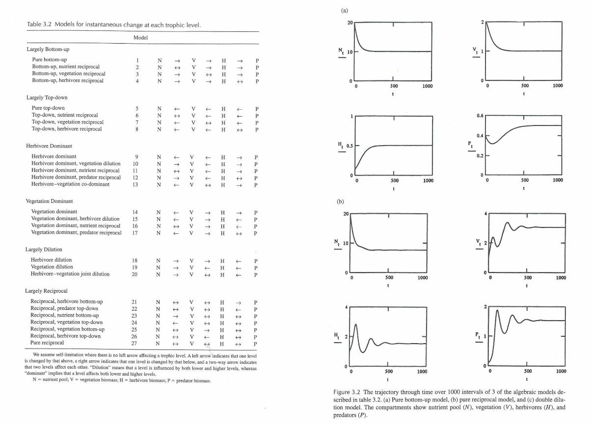
Table 3.2 Models for instantaneous change at each trophic level.

Largely Bottom-up

Pure bottom-up Bottom-up, nutrient reciprocal Bottom-up, vegetation reciprocal Bottom-up, herbivore reciprocal

Largely Top-down

Pure top-down Top-down, nutrient reciprocal Top-down, vegetation reciprocal Top-down, herbivore reciprocal

Herbivore Dominant

Herbivore dominant Herbivore dominant, vegetation dilution Herbivore dominant, nutrient reciprocal Herbivore dominant, predator reciprocal Herbivore-vegetation co-dominant

Vegetation Dominant

Vegetation dominant Vegetation dominant, herbivore dilution Vegetation dominant, nutrient reciprocal Vegetation dominant, predator reciprocal

Largely Dilution

Herbivore dilution Vegetation dilution Herbivore-vegetation joint dilution

Largely Reciprocal

Reciprocal, herbivore bottom-up Reciprocal, predator top-down Reciprocal, nutrient bottom-up Reciprocal, vegetation top-down Reciprocal, vegetation bottom-up Reciprocal, herbivore top-down Pure reciprocal

Model

2 3 4

5 6 7 8

9 10 ll 12 13

14 15 16 17

18 19 20

21 22 23 24 25 26 27

N N N N

N N N N

N N N N N

N N N N

N N N

N N N N N N N

v v v v

v v v v

v v v v v

v v v v

v v v

v v v v v v v

H H H H

H H H H

H H H H H

H H H H

H H H

H H H H H H H

p p p p

p p p p

p p p p p

p p p p

p p p

p p p p p p p

We assume self-limitation where there is no left arrow affecting a trophic level. A left arrow indicates that one level is changed by that above, a right arrow indicates that one level is changed by that below, and a two-way arrow indicates that two levels affect each other. "Dilution" means that a level is influenced by both lower and higher levels, whereas "dominant" implies that a level affects both lower and higher levels.

N = nutrient pool; V = vegetation biomass; H = herbivore biomass; P = predator biomass.

(a)

20 r-------,.-----,

N, 10~----------~

(b)

o~----~1---~ 0 soo 1000

1 ~----~.---~

0

I soo 1000

20r------~.----~

N, !Ol ~--------------~

-

oL-------~·~------~ 0 soo 1000

oL-----~------~ 0 soo 1000

~ :~~----·------~ 0~------~-~------~

0 soo 1000

0 soo 1000

4~--------,---------~

oL-_____ _. ______ ~ 0 soo 1000

1000

Figure 3.2 The trajectory through time over 1000 intervals of 3 of the algebraic models de­scribed in table 3.2. (a) Pure bottom-up model, (b) pure reciprocal model, and (c) double dilu­tion model. The compartments show nutrient pool (N), vegetation (V), herbivores (H ), and predators (P).

36 ECOSYSTEM DYNAMICS OF THE BOREAL FOREST

(c)

20r-------~.--------~

N, 10~'---------------~ 0~------~·------~

0 soo 1000

oL-------~~------~ 0 soo 1000

Figure 3.2 continued

The 27 possible ways trophic levels can interact directly with each other can be con­veniently grouped by the dominant direction of control in the system and by the dominant trophic level. Although other groupings can be produced just as easily, we prefer the six groups described next and shown in table 3.2.

3.2. 1 Bottom-up Models

Bottom-up models have an uninterrupted direction of control from lower to higher lev­els (figure 3.2a). They all predict that nutrient availability determines the biomass in the higher levels and thus assume that supply of nutrients is limiting.

Such models, therefore, would be most relevant in nutrient-poor environments where plants have difficulty obtaining nutrients. In terrestrial system~ this would apply to polar tundra (L. Oksanen 1988, 1990), subarctic boreal forests with acldic soils (this study), and nutrient-poor sclerophyll forests in Australia. The soils of much of Australia are so poor that nutrient content of leaves in individual trees and the densities of mammalian fo­liovores reflect the local nutrient condition of the soil the trees grow in (Braithwaite et al. 1983, Braithwaite 1996). In aquatic systems nutrients are low in high-latitude, cold oligo­trophic lakes, in acidic marshes and peat bogs, and in warm open-ocean systems.

TROPHIC INTERACTIONS AND COMMUNITY ORGANIZATION 37

3.2.2 Top-down Models

Top-down models have an uninterrupted direction of control from the top level down­ward. Thus, predators control the herbivore biomass, and herbivores control plant bio­mass. They all predict that nutrients are not limiting and that community structure is de­termined by type of predator species and predation.

These models could be applicable to aquatic systems, particularly the more eutrophic lakes with many trophic levels. Larger fish species determine the presence or absence of small fish species, which in turn determine which zooplankton occur (Menge and Suther­land 1976, Estes et al. 1977, Simenstad et al. 1978, Paine 1980, Power 1990, Menge 1992, Carpenter and Kitchell1993, Rosemund et al. 1993, Wootton 1994a).

3.2.3 Herbivore-dominated Models

In herbivore-dominated models the herbivore level controls both the predator and plant levels. Interactions between plants and nutrients can be either top-down or bottom-up. These would apply to systems where herbivores dominate. Generally, such systems are grasslands. In tropical savannas, such as the Serengeti, large grazing mammals structure the vegetation and determine predator biomass (McNaughton 1985, Semmartin and Oesterheld 1996). Predators do not limit the dominant herbivores (Sinclair 1975, Sinclair and Arcese 1995). The dominant effects of herbivores are also seen in temperate prairies (Huntly 1991) and in arctic and antarctic tundra (Leader-Williams 1988, Albon and Lang­vatn 1992). In many of these systems, the large mammalian herbivores become numerous and develop seasonal migrations.

3.2.4 Vegetation-dominated Models

Vegetation-dominated models predict that soil nutrients are determined by plant bio­mass and that herbivores are limited by food supply. Such models would apply to forests where trees dominate the biomass. In particular, tropical forests absorb most of the nutri­ents in the soil, leaving the soil low in nutrients (Connell1978). At the same time, herbi­vores in these forests, largely insects, consume only a small fraction of the vegetation be­cause plants are protected by structural and chemical defenses (Reichle et al. 1973, Sinclair 1975). Similar processes occur in temperate forests (Feeny 1968).

One model (1 3) has both vegetation and herbivores as codominants. This would pre­dict high vegetation biomass, but its structure would be strongly influenced by herbivores because of its high palatability. Such special conditions are not obviously identified in na­ture, but may reprasent subarctic and alpine systems where vegetation and herbivores dominate (Oksanen et al. 1981, Batzli 1983, Keith 1983, Fretwell1987, L. Oksanen 1990, Moen et al. 1993, Marquis and Whelan 1994, Krebs et al. 1995).

3.2.5 Dilution Models

Dilution models imply that both the lower and higher levels limit the intermediate trophic level. Thus, there are both bottom-up and top-down effects (figure 3.2c). Such a process may be seen in aquatic systems, where both nutrient content of lakes and the

38 ECOSYSTEM DYNAMICS OF THE BOREAL FOREST

predator community affect trophic dynamics (McQueen et al. 1986, 1989). Insect-para­sitoid-dominated systems may also be dilution systems, where parasitoids control her­bivorous insects and nutrients control vegetation, which in turn affects herbivores (Law­ton and Strong 1981, Strong et al. 1984, Price eta!. 1990, Gomez and Zamora 1994).

3.2.6 Reciprocal Models

Reciprocal models suggest that there are two-way interactions between most of the trophic levels. The last model (27; figure 3.2b) predicts reciprocal effects at all levels. These models, therefore, could apply to most ecosystems.

3.3 Experimental Pertu rbations in the Boreal Forest

We tested the models described above using experimental perturbations of the boreal forest food web. The models can be distinguished by unique sets of predictions produced from seven perturbations that systematically reduced or enhanced each trophic level. The predictions were concerned with the subsequent direction of change in the populations or biomass of other levels. The main components of the system are described elsewhere, but in essence the plant level is characterized by herbaceous dicots, woody shrubs such as wil­low and birch, and white spruce. The herbivore level is dominated by the snowshoe hare, which exhibits a 10-year cycle of abundance, and by ground squirrels, red squirrels, and various vole species. The predator level is composed of carnivores such as lynx and coy­ote and various raptors, notably the great horned owl.

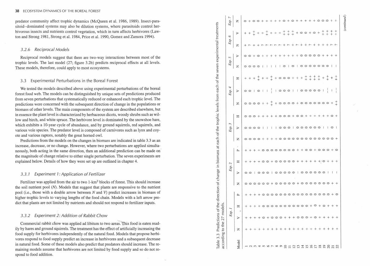
Predictions from the models on the changes in biomass are indicated in table 3.3 as an increase, decrease, or no change. However, where two perturbations are applied simulta­neously, both acting in the same direction, then an additional prediction can be made on the magnitude of change relative to either single perturbation. The seven experiments are explained below. Details of how they were set up are outlined in chapter 4.

3.3. 1 Experiment 1: Application of Fertilizer

Fertilizer was applied from the air to two l-km2 blocks of forest. This should increase the soil nutrient pool (N). Models that suggest that plants are responsive to the nutrient pool (i.e. , those with a double arrow between N and V) predict increases in biomass of higher trophic levels to varying lengths of the food chain. Models with a left arrow pre­dict that plants are not limited by nutrients and should not respond to fertilizer inputs.

3.3.2 Experiment 2: Addition of Rabbit Chow '--.

Commercial rabbit chow was applied ad libitum to two areas.'Crhis food is eaten read-ily by hares and ground squirrels. The treatment has the effect of artificially increasing the food supply for herbivores independently of the natural food. Models that propose herbi­vores respond to food supply predict an increase in herbivores and a subsequent decrease in natural food. Some of these models also predict that predators should increase. There­maining models assume that herbivores are not limited by food supply and so do not re­spond to food addition.

"' c Q)

E -~ a. X Q)

c Q)

> Q) V'>

Q)

-5 """ 0 ..r:::. u "' Q)

E e

""" V'>

Q)

> j,!

.!::!

..r:::. a. e ..... Q)

-5 0 ..r:::. u

"' Q)

-;;; V'> V'>

"' E .Q .D c

~ c

"' ..r:::. u

""" 0 c 0 ·e ~

Q) "' ..r:::.-..... Q)

""" "'0 0 0 ~ E or-....

'_;j N .!::! Q) -o..r:::.

Q) ..... .... 0

Cl..+-'

Moo 0 c

M'O Q) ....

- 0 .D u ~ ~

o + oo +++++ o + o +++++ ooo ++

> + + + + + + + + + + + 00 + 0 + + + + + ++ + + +++ ++++

z

> oo+o ++ + +++++ +ooooo+ +++

z o o o o I I I I O I O I OOOOOOO

..,.. ++++ + +++ooo++++++ +++++ ..... + + ++++ + +

> oo I o I I I OOO I I OOOOO I

z oooo ++!+o ooo+ooooooo +!

ooo+ ++++ ooo + oo ++++++ o +

> 0000 1 III OOO I OOOOOOI I O I

z oooo++ ++o oooooooooooo +

+ +++ oooooooo ++o o + ooo+o

++++ oo + ooooo++ ++++ o +++

> OO I OOO I OOOOO I OOOOOO I I I

z oooooo + ooooo+ooooooo ++

+++ + oooooooooooooooo + o

++++ ooooooooooo + O + o +++

> ++ ++o + ooo+++ooo + o +++++

z +++ + ++++++++ + +++++++++

-N~~~~~oo~o-N~V~~~~~o - N --- -------NNN

('..

~ z 0 + + + +

> + + + + + '0 + + +

~ z + <:-· C'-· C'-· C"-·

"' > + + 0 + +

~ z 0 I 0

::r: + + + + + + + + +

"t'

~ > 0 I

z 0 +o + + + +

::r: + + + + +

""' ~ > I I 0 I I

z 0 +o + +

Q., + + + 0 +

N ::r: + + + 0 +

~ > I I 00 I

z 0 + oo +

Q., + 0 + 0 +

::r: + 0 + 0 + -. .:0 ~ CIJ ::J > + 0 + + + .s t ~ z + + + + + ~ M

CIJ ..., :::0 -o

~ 0

~~~~N ::E

6 0 ~ > 0

c: .8 "' >< ~ II .g ~ 0

s~~e~ "'- - "'E -o~fi~a ~~§~-o II .g ~ .g ~

'V co .... 0 ~ . C) 0 :.a 0 e- ~ ~ f:? -~

viu.l>'Q6"~ ~ .,; II "' c ..c E5r---~urv

.9 ~ ci. E C; -5

.0 - )( 0 ';i ..... C>~UJ:o-oS ~ Q) ~ c ~ Cl)

]o1:loo.g ~ ., ;.::: g ~ 'fl o..~ e ::=:.a :.a II o.~ 4) E ~ .

""- II + ~ ~ ~-iJ ~M~ge-g.£ ~g.~-o£Ut; :.c;wo ll ~~-&, o r: ~ 1 ·e :c o .g ~ I :.= ~ ~ :E:.O.t:t>~~-5 ~~~~+go_ ..c~\O +~::i"'2 11 ~g.vg~S

=:t": n UJ~~..c~ ~ N PI t e ~ .g ~ ';:3~0. - (,)

5~6~".2S:.a :.stzJ .. u ~~~ ~ g g ~ e ~ ·e ~ -~ :~ ~ ~ ~ Vi .g ~ "'C v ::s o-o..cu~~1j ~ ~ II J G) c f,;,

>1:!.,., :oe,o. II :.:: · V' !9 ... _. t; > ·e ~ ~ .o ~ ~ .• .,wo:O E: 8 c.;, .. () Q) Q)

o. II § .5 g. g ~ ... -:E~::s~g fi C ~ «S II v ·~ 'E E co ~ C'o· -5 i)

;::) ] · - "'0 c 00 c ·c .o ·- 4)

118.""11~-~ ~ z~++~..!l~

~ ~ «< ~ "" u -5 v

TROPHIC INTERACTIONS AND COMMUNITY ORGANIZATION 41

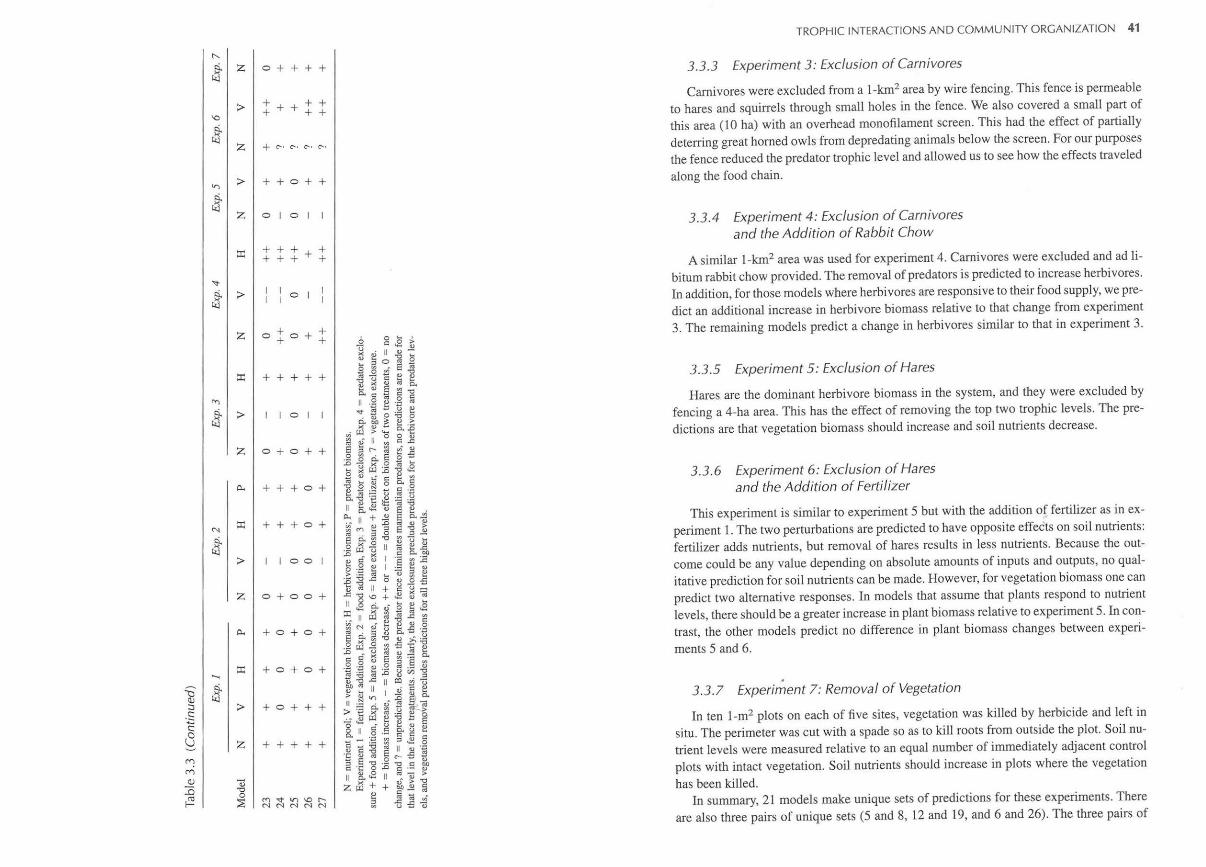
3.3.3 Experiment 3: Exclusion of Carnivores

Carnivores were excluded from a 1-km2 area by wire fencing. This fence is permeable to hares and squirrels through small holes in the fence. We also covered a small part of this area (10 ha) with an overhead monofilament screen. This had the effect of partially deterring great horned owls from depredating animals below the screen. For our purposes the fence reduced the predator trophic level and allowed us to see how the effects traveled

along the food chain.

3.3.4 Experiment 4: Exclusion of Carnivores and the Addition of Rabbit Chow

A similar l-km2 area was used for experiment 4. Carnivores were excluded and ad li­bitum rabbit chow provided. The removal of predators is predicted to increase herbivores. In addition, for those models where herbivores are responsive to their food supply, we pre­dict an additional increase in herbivore biomass relative to that change from experiment 3. The remaining models predict a change in herbivores similar to that in experiment 3.

3.3.5 Experiment 5: Exclusion of Hares

Hares are the dominant herbivore biomass in the system, and they were excluded by fencing a 4-ha area. This has the effect of removing the top two trophic levels. The pre­dictions are that vegetation biomass should increase and soil nutrients decrease.

3.3.6 Experiment 6: Exclusion of Hares and the Addition of Fertilizer

This experiment is similar to experiment 5 but with the addition of fertilizer as in ex­periment 1. The two perturbations are predicted to have opposite effects on soil nutrients: fertilizer adds nutrients, but removal of hares results in less nutrients. Because the out­come could be any value depending on absolute amounts of inputs and outputs, no qual­itative prediction for soil nutrients can be made. However, for vegetation biomass one can predict two alternative responses. In models that assume that plants respond to nutrient levels, there should be a greater increase in plant biomass relative to experiment 5. In con­trast, the other models predict no difference in plant biomass changes between experi­

ments 5 and 6.

3.3.7 Experi~ent 7: Removal of Vegetation

In ten 1-m2 plots on each of five sites, vegetation was killed by herbicide and left in situ. The perimeter was cut with a spade so as to kill roots from outside the plot. Soil nu­trient levels were measured relative to an equal number of immediately adjacent control plots with intact vegetation. Soil nutrients should increase in plots where the vegetation

has been killed. In summary, 21 models make unique sets of predictions for these experiments. There

are also three pairs of unique sets (5 and 8, 12 and 19, and 6 and 26). The three pairs of

42 ECOSYSTEM DYNAMICS OF THE BOREAL FOREST

models with the same predictions occur because one perturbation is missing from our bo­real forest experiments (for logistical reasons): the direct addition of herbivores. If this ex­periment had been achieved, then all these models could have been discriminated.

3.4 Discussion

3.4. 1 Limitations of the Models

We employed both removal and addition experiments. Removal experiments are more powerful because, to analyze the effect of a factor, it must be removed. Addition experi­ments are not the reverse of removals (Royama 1977), but they are necessary in this con­text to determine the presence of right-arrow regulatory effects. The double perturbation experiments where both addition and removal were applied allow us to evaluate the rela­tive strengths of simultaneous top-down and bottom-up effects.

In general, the most informative experiments are those that influence higher rather than lower trophic levels. This is because perturbations at lower levels do not necessarily feed up-only some models predict this result. In contrast, perturbations on higher levels should always feed down to lower levels.

Our assumptions of the effect of food addition may be incorrect in two ways. One pos­sibility is that rabbit chow could act more as an attractant, causing hares and other species to commute to the food from outside the experimental area. Such commuting would have the effect of increasing the herbivore trophic level directly through a behavioral response instead of through a reproductive response to food. A second possibility is that food ad­dition would attract herbivores to eat more of the artificial food and so would decrease the impact of herbivores on the vegetation. In both cases predictions can be altered accord­ingly, and the number of unique sets does not alter.

We started this analysis of models and their predictions by assuming simple linear, first order interactions. Many other models, including nonlinear interactions, such as saturat­ing functional responses, could also be suggested, and this would be the next step. We con­sider that these more complex models would lead to basically similar predictions. We started with experimental tests of simple models because they are easier to reject than complex models. We should first test simple models with our results before turning to complex models (Hairston and Hairston 1997). Density manipulation experiments in these different ecosystems is the most effective way of determining the generality of these top­down and bottom-up models (Dwyer 1995).

3.4.2 Models of Trophic-/eve/ Interactions in Different Ecosystems

Although we cannot yet assign individual models to particular ecosystems, we can speculate on the classes of models that may be applitable in different ecosystems. Nutrient­poor sclerophyll forests such as those of Australia have strong bottom-up effects (Braith­waite et al. 1983, Braithwaite 1996) and would be largely represented by right-arrow models such as 1-4, 16, 20-23, and 25. Tropical forests, where vegetation dominates (Connell 1978, 1983), could be represented by models 14-17, 21- 22, and 24 - 25.

TROPHIC INTERACTIONS AND COMMUNITY ORGANIZATION 43

In subarctic tundra systems, where vegetation and herbivores dominate (Oksanen et al. 1981, Fretwell 1987, L. Oksanen 1990, Moen et al. 1993, Marquis and Whelan 1994, Krebs et al. 1995), models 9-17 could apply. As one moves to lower latitudes, such as in the temperate grasslands of the North American prairies (Huntly 1991) and in the tropi­cal savannas of the Serengeti (Sinclair 1975, McNaughton 1985, Sinclair and Arcese 1995), herbivores dominate, and models with arrows leading from the herbivores could apply (e.g., models 9- 13,21, 23-24, and 26).

Both bottom-up and top-down (dilution) effects at the herbivore level could operate in insect herbivores (models 15- 18, and 20) (Hairston et al. 1960, McQueen et al. 1986, Pace and Funke 1991, Harrison and Cappuccino 1995). However, insect-dominated systems may also be controlled by predators or parasitoids (Lawton and Strong 1981, Strong et al. 1984, Price et al. 1990, Gomez and Zamora 1994, Spiller and Schoener 1994, Floyd 1996, Moran and Hurd 1998), and models 5- 8,22, 24, and 26 might apply.

In aquatic ecosystems, models with mainly left arrows (largely top-down effects; e.g., 5-8, 22, 24, and 26) may apply (Menge and Sutherland 1976, Estes et al. 1977, Simen­stad et al. 1978, Paine 1980, McQueen et al. 1986, Power 1990, Menge 1992, 1995, Car­penter and Kitchell1993, Rosemund et al. 1993, Wootton 1994a). Indirect effects are well known in aquatic and marine systems (Schoener 1993, Wootton 1993, 1994b, Menge 1997) but far less evident in terrestrial systems. The most general of the models is 27, the pure reciprocal model, because it could represent many if not all ecosystems.

3.5 Summary

Models of community organization involve variations of the top-down (predator con­trol) or bottom-up (nutrient limitation) hypotheses. Verbal models, however, can be inter­preted in different ways, leading to confusion. Therefore, we predict from first principles the range of possible trophic-level interactions and define mathematically the instantaneous effects of experimental perturbations. Some of these interactions are logically and biolog­ically unfeasible. The remaining set of 27 feasible models is based on an initial assump­tion, for simplicity, of linear interactions between trophic levels. Many more complex and nonlinear models are logically feasible but, for parsimony, simple ones are tested first.

We have described a series of seven experiments designed to test the predictions of the models and distinguish between them. These experiments were conducted on the verte­brate community in the boreal forest at Kluane, Yukon. With these experiments we can distinguish 21 models and 3 pairs of models, giving 24 unique sets of predictions. In chap­ter 17 we apply these models to the results discussed in detail in the intervening chapters of this book.

Literature Cited

Abrams, P. A. 1993. Effect of increased productivity on the abundances of trophic levels. Amer­ican Naturalist 141:351-371.

Albon, S.D., and R. Langvatn. 1992. Plant phenology and the benefits of migration in a tem­perate ungulate. Oikos 65:502-513.

44 ECOSYSTEM DYNAMICS OF THE BOREAL FOREST

Arditi, R., and L. R. Ginsburg. 1989. Coupling in predator-prey dynamics: ratio-dependence. Journal of Theoretical Biology 139:311-326.

Arditi, R., L. R. Ginsburg, and H. R. Akcakaya. 1991. Variation in plankton densities among lakes: a case for ratio-dependent predation models. American Naturalist 138:1287- 1296.

Batzli, G. 0. 1983. Responses of arctic rodent to nutritional factors. Oikos 40:396-406. Bell, R.H.V. 1982. The effect of soil nutrient availability on community structure in African

ecosystems. in B. J. Huntley and B. H. Walker (eds). Ecology of tropical savannas, pages 193-216. Springer-Verlag, New York.

Botkin, D. B., J. M. Mellilo, and L. S-Y. Wu. 1981. How ecosystem processes are linked to large mammal population dynamics. in C. W. Fowler and T. D. Smith (eds). Dynamics of large mammal populations, pages 373-387. Smith, John Wiley and Sons, New York.

Braithwaite, L. W. 1996. Conservation of arboreal herbivores: the Australian scene. Australian Journal of Ecology 21:21-30.

Braithwaite, L. W. , M. L. Dudzinski, and J. Turner. 1983. Studies of the arboreal eucalypt forests being harvested for wood pulp at Eden, New South Wales. II. Relationship between the fauna density, richness and diversity and measured variables of habitat. Australian Wildlife Research 10:231-247.

Briand, F., and J. E. Cohen. 1987. Environmental correlates of food chain length. Science 238:956-960.

Carpenter, S. R., and J. F. Kitchell. 1987. The temporal scale of variance in limnetic primary production. American Naturalist 129:417- 433.

Carpenter, S. R., and J. F. Kitchell. 1988. Consumer control of lake productivity. Bioscience 38:764-769.

Carpenter, S. R., and J. F. Kitchell (eds). 1993. The trophic cascade in lakes. Cambridge Uni­versity Press, Cambridge.

Carpenter, S. R., J. F. Kitchell, and J. R. Hodgson. 1985. Cascading trophic interactions and lake productivity. BioScience 35:634- 639.

Caughley, G. 1976. Plant-herbivore systems. in R. M. May (ed). Theological history, pages 94-113. Saunders, Philadelphia.

Coe, M. J., D. H. Cumming, and J. Phillipson. 1976. Biomass and production of large African herbivores in relation to rainfall and primary production. Oecologia 22:314- 354.

Cohen, J. E. 1978. Food webs and niche space. Princeton University Press, Princeton, New Jer­sey.

Connell, J. H. 1978. Diversity in tropical rainforests and coral reefs. Science 199: 1302- 1310. Connell, J. H. 1983. On the prevalence and relative importance of interspecific competition:

evidence from field experiments. American Naturalist 122:661-696. Dwyer, G. 1995. Simple models and complex interactions. inN. Cappuccino and P. W. Price

(eds). Population dynamics: new approaches and synthesis, pages 209-227. Academic Press, New York.

Estes, J. A., and D. 0. Duggins. 1995. Sea otters and kelp forests in Alaska: generality and vari­ation in a community ecological paradigm. Ecological Monographs 65:75-100.

Estes, J. A., D. 0. Duggins, and G. B. Rathbun. 1989. The ecology of extinctions in kelp for­est communities. Conservation Biology 3:252- 264.

Estes, J. A., N. S. Smith, and J. F. Palmisano. 1977- Sea otter predation and community orga­nization in the Western Aleutian Islands, Alaska. Ecology 59:822-833.

Feeny, P. P. 1968. Effect of oak leaf tannins on larval growth of the winter moth Operophtera brumata. Journal oflnsect Physiology 14:801- 817.

Floyd, T. 1996. Top-down impacts on creosotebush herbivores in a spatially and temporally complex environment. Ecology 77:1544-1555.

TROPHIC INTERACTIONS AND COMMUNITY ORGANIZATION 45

Fretwell, S. D. 1977. The regulation of plant communities by food chains exploiting them. Per­spectives in Biology and Medicine 20:169-185.

Fretwell, S.D. 1987. Food chain dynamics: the central theory of ecology? Oikos 50:291-301 . Gomez, J. M., and R. Zamora. 1994. Top-down effects in a tritrophic system: parasitoids en­

hance plant fitness. Ecology 75:1023-1030. Hairston, N. G. , and N. G. Hairston. 1997. Does food web complexity eliminate trophic-level

dynamics? American Naturalist 149:1001- 1007. Hairston, N. G., F. E. Smith, and L. B. Slobodkin. 1960. Community structure, population con­

trol and competition. American Naturalist 94:421-425. Hall, S. J ., and D. Raffaelli. 1991. Food-web patterns: lessons from a species-rich web. Jour­

nal of Animal Ecology 60:823-842. Hanski, I. 1991. The functional response of predators: worries about scale. Trends in Ecology

and Evolution 6: 141 - 142. Harrison, S., and N. Cappuccino. 1995. Using density-manipulation experiments to study pop­

ulation regulation./n N. Cappuccino and P. W. Price (eds). Population dynamics: new ap­proaches and synthesis, pages 131-148. Academic Press, New York.

Hawkins, B. A. 1992. Parasitoid-host food web and donor control. Oikos 65:159-162. Houston, D. B. 1982. The northern Yellowstone elk: ecology and management. MacMillan,

London. Hunter, M. D., and P. W. Price. 1992. Playing chutes and ladders: bottom-up and top-down

forces in natural communities. Ecology 73:724-732. Huntly, N. 1991. Herbivores and the dynamics of communities and ecosytems. Annual Review

of Ecology and Systematics 22:477-503. Keiter, R. B., and M.S. Boyce. 1991. The greater Yellowstone ecosystem: redefining Amer­

ica's wilderness heritage. Yale University Press, New Haven, Connecticut. Keith, L. B. 1983. Role of food in hare population cycles. Oikos 40:385-395. Krebs, C. J., S. Boutin, R. Boonstra, A. R. E. Sinclair, J. N. M. Smith, M. R. T. Dale, K. Mar­

tin, and R. Turkington. 1995. Impact of food and predation on the snowshoe hare cycle. Science 269:1112- 1115.

Laurenson, M. K. 1995. Implications for high offspring mortality for cheetah population dy­namics. in A.R.E. Sinclair and P. Arcese (eds). Serengeti II: dynamics, management and conservation of an ecosystem, pages 385-399. University of Chicago Press, Chicago.

Lawton, J. H. 1989. Food webs. in J. M. Cherrett (ed). Ecological concepts, pages 43-78. Blackwell Scientific Publications, Oxford.

Lawton, J. H., and D. R. Strong. 1981. Community patterns and competition in folivarous in­sects. American Naturalist 118:317-338.

Leader-Williams, N. 1988. Reindeer on South Georgia: the study of an introduced population. Cambridge University Press, Cambridge.

Marquis, R. J. , and Whelan, C. J. 1994. Insectivorious birds increase growth of white oak through consumption of leaf-chewing insects. Ecology 75:2007-2014.

McLaren, B. E., and It 0. Peterson. 1994. Wolves, moose and tree rings on Isle Royale. Sci­ence 266:1555-1557.

McNaughton, S. J. 1985. Ecology of a grazing ecosystem: the Serengeti. Ecological Mono­graphs 55:259-294.

McNaughton, S. J. , M. Osterheld, D. A. Frank, and K. J. Will iams. 1989. Ecosystem level pat­terns of primary productivity and herbivory in terrestrial habitats. Nature 341:142-144.

McQueen, D. G., M. R. S. Johannes, J. R. Post, T. J. Stewart, and D. R. S. Lean. 1989. Bot­tom-up and top-down impacts on freshwater pelagic community structure. Ecological Monographs 59:289-309.

46 ECOSYSTEM DYNAMICS OF THE BOREAL FOREST

McQueen, D. G. , J. R. Post, and E. L. Mills. 1986. Trophic relationships in freshwater pelagic ecosystems. Canadian Journal of Fisheries and Aquatic Sciences 43: 1571- 1581.

Mduma, S. A. R. , A. R. E. Sinclair, and R. Hilborn. 1999. Food regulates the Serengeti wilde­beest: a forty-year record. Journal of Animal Ecology 68: 1101- 1122.

Menge, B. A. 1992. Community regulation: under what conditions are bottom-up factors im­portant on rocky shores? Ecology 73:755 - 765.

Menge, B. A. 1995. Indirect effects in marine rocky intertidal interaction webs: patterns and importance. Ecological Monographs 65:21-74.

Menge, B. A. 1997. Detection of direct versus indirect effects: were experiments long enough? American Naturalist 149:801- 823.

Menge, B. A., and T. M. Farrell. 1989. Community structure and interaction webs in shallow marine hard-bottom communities: tests of an environmental stress model. Advances in Ecological Research 19:189-262.

Menge, B. A., and A.M. Olsen. 1990. Role of scale and environmental factors in regulation of community structure. Trends in Ecology and Evolution 5:52- 57.

Menge, B. A., and J.P. Sutherland. 1976. Species diversity gradients: synthesis of the roles of predation, competition and temporal heterogeneity. American Naturalist 110:351-369.

Merrill, E. H., N. L. Stanton, and J. C. Hilc 1994. Responses of bluebunch wheatgrass, Idaho fescue, and nematodes to ungulate grazing in Yellowstone National Park. Oikos 69:231-240.

Moen, J. , H. Gardfjell , L. Oksanen, L. Ericson, and P. Ekerholm. 1993. Grazing by food-lim­ited microtine rodents on a productive experimental plant community: does the "green desert" exist? Oikos 68:401 - 413.

Moran, M. D., and L. E. Hurd. 1998. A trophic cascade in a diverse arthropod community caused by a generalist arthropod predator. Oecologia 113:126- 132.

Oksanen, L. 1988. Ecosystem organization: mutualism and cybernetics or plain Darwinian struggle for existence? American Naturalist 131:424- 444.

Oksanen, L. 1990. Predation, herbivory, and plant strategies along gradients of primary pro­ductivity. in D. Tilman and J. Grace (eds). Perspectives on plant consumption, pages 445-474. Academic Press, New York.

Oksanen, L., and L. Ericson. 1987. Concluding remarks: trophic exploitation and community structure. Oikos 50:417-422.

Oksanen, L. , S. D. Fretwell, J. Arruda, and P. Niemala. 1981. Exploitation ecosystems in gra­dients of primary productivity. American Naturalist 118:240- 261.

Oksanen, T. 1990. Exploitation ecosystems in heterogeneous habitat complexes. Evolutionary Ecology 4:220-234.

Pace, M. L., and E. Funke. 1991. Regulation of planktonic microbial communities by nutrients and herbivores. Ecology 72:904- 914.

Paine, R. T. 1980. Food webs: linkage, interaction strength and community infrastructure. Jour­nal of Animal Ecology 49:667-685.

Paine, R. T. 1988. Food webs: road maps of interactions or grist for theoretical development? Ecology 69: 1648-1654.

Pimm, S. L. 1982. Food webs. Chapman and Hall, London. Polis, G. A. 1991. Complex trophic interactions in deserts: an empirical critique of food web

theory. American Naturalist 138:123- 155. '<.,

Power, M. E. 1984. Depth distributions of armoured catfish: predator-induced resource avoid­ance? Ecology 65:523-528.

Power, M. E. 1990. Effects of fish in riverfood webs. Science 250:811 - 814. Price, P. W., N . Cobb, T. P. Craig, G. W. Fernandes, J. K. Itarni , S. Mopper, and R. W. Preszler.

1990. Insect herbivore population dynamics on trees and shrubs: new approaches relevant

TROPHIC INTERACTIO NS AND COMMUNITY ORGAN IZATION 47

to latent and eruptive species and life table development. in E. A. Bernays (ed). Insect­plant interactions, volume 2, pages 1-38. CRC Press, Boca Raton, Florida.

Reichle, D. E. , R. A. Goldstein, R. I. Van Hook, and G. J. Dodson. 1973. Analysis of insect consumption in a forest canopy. Ecology 54: 1076- 1084.

Rosemund, A. D., P. J. Mulholland, and J. W. Elwood. 1993. Top-down and bottom-up control of stream periphyton: effects of nutrients and herbivores. Ecology 74:1264- 1280.

Royama, T. 1977. Population persistence and density dependence. Ecological Monographs 47:1-35.

Schmitz, 0. J. 1998. Direct and indirect effects of predation and predation risk in old-fie ld in­teraction webs. American Naturalist 151:327-342.

Schoener, T. 1989. Food webs from the small to the large. Ecology 70:1559-1589. Schoener, T. W. 1993. On the relative importance of direct versus indirect effects in ecological

communities. in H. Kawanabe, J. E. Cohen, and K. Iwasaki (eds). Mutualism and com­munity organization: behavioral , theoretical and food-web approaches, pages 365- 4 11. Oxford University Press, New York.

Schoen1y, K. , R. A. Beaver, and T. A. Heumier. 1991. On the trophic relations of insects: a food­web approach. American Naturalist 137:597-638.

Semmartin, M., and M. Oesterheld. 1996. Effect of grazing pattern on primary productivity. Oikos 75:431- 436.

Simenstad, C. A. , J. A. Estes, and K. W. Kenyon. 1978. Aleuts, sea otters and alternate stable state communities. Science 200:403 - 4 11.

Sinclair, A. R. E. 1975. The resource limitation of trophic levels in tropical grassland commu­nities. Journal of Animal Ecology 44:497-520.

Sinclair, A. R. E. 1995. Serengeti past and present. in A. R. E. Sinclair and P. Arcese (eds). Serengeti II: Dynamics, management and conservation of an ecosystem, pages 1- 30. Uni­versity of Chicago Press, Chicago.

Sinclair, A. R. E. , and P. Arcese (eds). 1995. Serengeti II: dynamics, management and conser­vation of an ecosystem. University of Chicago Press, Chicago.

Sinclair, A. R. E. , C. J. Krebs, J. M. Fryxel, R. Turkington, S. Boutin, R. Boonstra, P. Seccombe­Hett, P. Lundberg, and L. Oksanen. 2000. Testing hypotheses of trophic level interactions: a boreal forest ecosystem. Oikos 89:313-328.

Singer, F. J. , L. C. Mark, and R. C. Cates. 1994. Ungulate herbivory of willows on Yellow­stone's northern winter range. Journal of Range Management 47:435- 443.

Slobodkin, L. B., F. E. Smith, and N. G. Hairston. 1967. Regulation in terrestrial ecosystems, and the implied balance of nature. American Naturalist 101:109-124.

Spiller, D. A. , and T. W. Schoener. 1994. Effects of top and intermediate predators in a terres­trial food web. Ecology 75:182- 196.

Strong, D. R. 1992. Are trophic cascades all wet? Differentiation and donor-control in speciose ecosystems. Ecology 73:747- 754.

Strong, D. R. , D. Simberloff, L. G. Abele, and A. B. Thistle (eds). 1984. Ecological commu­nities: conceptual issues and the evidence. Princeton University Press, Princeton, New Jersey.

Walker, B. H. 1991. Biological diversity and ecological redundancy. Conservation Biology 6:18 - 23.

White, T. C. R. 1978. The importance of a relative shortage of food in animal ecology. Oeco­logia 3:71- 86.

White, T. C. R. 1984. The abundance of invertebrate herbivores in relation to the availability of nitrogen in stressed food plants. Oecologia 63:90- 105.

Wootton, J. T. 1993. Indirect effects and habitat use in an intertidal community: interaction chains and interaction modifications. American Naturalist 141:71- 89.

48 ECOSYSTEM DYNAMICS OF THE BOREAL FOREST

Wootton, J. T. 1994a. Predicting direct and indirect effects: an integrated approach using ex­periments and path analysis. Ecology 75:151- 165.

Wootton, J. T. 1994b. The nature and consequences of indirect effects in ecological communi­ties. Annual Review of Ecology and Systematics 25:443- 466.

Yodzis, P. 1988. The indeterminacy of ecological interactions as perceived through perturba­tion experiments. Ecology 69:508-515.