Numerical Approximations of a Tra c Flow Model on Networks

Numerical Approximations of a Traffic Flow

Model on Networks

Gabriella Bretti, Roberto Natalini, Benedetto Piccoli ∗

Abstract

We consider a mathematical model for fluid-dynamic flows on networkswhich is based on conservation laws. Road networks are considered asgraphs composed by arcs that meet at some junctions. The crucial pointis represented by junctions, where interactions occurr and the problemis underdetermined. The approximation of scalar conservation laws alongarcs is carried out by using conservative methods, such as the classical Go-dunov scheme and the more recent discrete velocities kinetic schemes withthe use of suitable boundary conditions at junctions. Riemann problemsare solved by means of a simulation algorithm which proceeds process-ing each junction. We present the algorithm and its application to somesimple test cases and to portions of urban network.

Key Words: scalar conservation laws, traffic flow, fluid-dynamic models,finite difference schemes, boundary conditions.

AMS Subject Classifications: Primary 65M06. Secondary 90B20, 35L65,34B45, 90B10.

∗Istituto per le Applicazioni del Calcolo “M. Picone”, Viale del Policlinico137, 00161 - Roma, Italy; E-mail: [email protected], [email protected],

[email protected]

1 Introduction.

The study of traffic flow aims to understand traffic behavior in urban context inorder to answer to several questions: where to install traffic lights or stop signs;how long the cycle of traffic lights should be; where to construct entrances,exits, and overpasses. The aims of this analysis are principally representedby the maximization of cars flow, and the minimization of traffic congestions,accidents and pollution. In general, network models of transportation systemsare assumed to be static, but these models do not allow a correct simulationof heavily congested urban road networks. For this reason, traffic engineershave started to consider some alternative models, often referred to as DTA(dynamic traffic assignment) or within-day models, see the review paper [2]and references therein. The use of within-day modeling makes necessary togive a new formulation of the problem: we have to solve the DNL (dynamicnetwork loading) problem, that is, the reproduction of the traffic flow motionon the network, which requires the introduction of time advancing mathematicalmodels (traffic simulation models). However, the main problems in DNL modelsare the fact that they do not properly reproduce the backward propagation ofshocks and the difficulty of collecting experimental data to test the models.Microscopic models, which form a widely used class of models, are characterizedby the fact that they are sensitive to small perturbations. On the other hand, itcan be difficult to give a qualitative description and visualization of phenomenaon a macroscopic scale.Here we deal with the fluid-dynamic models proposed in [7, 8], which can beseen as a macroscopic model with some traffic regulation strategies (within-daymodels) and which allows to observe the network in the time evolution throughwaves formation. In the 1950s James Lighthill and Gerald Whitham in [16],and independently Richards in [18], proposed to apply fluid dynamics conceptsto traffic. In a single road, this nonlinear model is based on the conservation ofcars described by the scalar hyperbolic conservation law:

∂tρ+ ∂xf(ρ) = 0, (1.1)

where ρ = ρ(t, x) ∈ [0, ρmax] is the density of cars, (t, x) ∈ R2 and ρmax > 0is the maximum density of cars on the road. The function f(ρ) is the flux ofcars, which is written as product of the density and of the local speed of carsv: i.e. f(ρ) = ρv. In most cases, and at least as a first order approximation,one can assume that v is a decreasing function, only depending on the density,and that the corresponding flux is a concave function. We refer to [12, 19]for more details and comments on the single road models. Let us remark thatfluid-dynamic models for traffic flow seem to be the most appropriate to detectmacroscopic phenomena as shocks formation and propagation of waves back-wards along roads. However, they can develop discontinuities in a finite timeeven starting from smooth initial data, then needing for a careful definition ofthe analytical framework, and an even greater consideration of suitable numer-ical schemes. We refer to [5, 9] for an updated account of the theory of generalhyperbolic conservation laws, and to [11, 15] for a standard introduction to the

1

main numerical ideas. Notice that, in all this classical works on traffic flows,only a single road was taken into account. More recently, in [7, 8, 13, 14], somemodels have been proposed for traffic flow on road networks. Following [8], wefocus on a road network composed by a finite number of roads parametrized byintervals [ai, bi] that meet at some junctions. Junctions play a key role, as thesystem at a junction is underdetermined even after prescribing the conservationof cars, that can be written as the Rankine-Hugoniot condition:

n∑

i=1

f(ρi(t, bi)) =

n+m∑

j=n+1

f(ρj(t, aj)),

where ρi, i = 1, . . . , n, are the car densities on incoming roads; ρj , j = n +1, . . . , n + m, are the car densities on outgoing roads. Such relation expressesthe equality of ingoing and outgoing fluxes. For endpoints that do not touch ajunction (and are not infinite), we assume to have a given boundary data andsolve the corresponding boundary problem, as in [4]. Let us remark that, in thispaper, traffic lights will not be considered, since their analytical and numericaltheory is already well understood [19].As in [8], we make the following two assumptions: there are some distributioncoefficients of traffic from incoming roads to outgoing roads; drivers behave insuch a way to maximize fluxes whenever is possible. One could also treat junc-tions where the number of incoming roads is greater than the number of outgoingones, not covered by the analysis of [8]. In particular, we are interested in thecase of two incoming and one outgoing roads. In this case, the two distributioncoefficients of the incoming roads must be equal to one, thus determining a lossof uniqueness for the solutions. This is not a purely mathematical issue, but itis rather due to the fact that if not all cars can go through the junction thenthere should be a yielding rule between incoming roads. To treat this case weintroduce a new parameter q ∈]0, 1[, the right of way (see [7]), which permits touniquely solve Riemann problems. In particular, it indicates which, among carspassing through the junction, is the percentage of cars coming from the firstincoming road and which is the percentage coming from the second road. Thedetails about the mentioned rules are discussed in Section 2.We deal with the numerical approximation of the possibly discontinuous solu-tions produced by this model. In particular, the main contribution of the paperis represented by the introduction of suitable boundary conditions at the junc-tions for classical and less classical numerical schemes. These schemes, namelyGodunov scheme and Kinetic methods, adapted to the problem, provide approx-imations which are quite stable as we will show later through many numericaltests.The paper is organized as follows. Section 2 is devoted to the description ofthe model. Some examples of simple networks are proposed in Section 3. InSection 4 we describe the numerical schemes with the particular boundary con-ditions used to produce approximated solutions of the problem. In Section 5 wegive an extended presentation of some numerical experiments which show theeffectiveness of our approximation.

2

2 Backgrounds

We consider the conservation of cars described by the equation [16, 18]:

∂tρ+ ∂xf(ρ) = 0, (2.1)

where ρ = ρ(t, x) is the density of cars, with ρ ∈ [0, ρmax], (t, x) ∈ R2 and ρmaxis the maximum density of cars on the road; f(ρ) is the flux, which can be writ-ten f(ρ) = ρv(ρ), with v(t, x) the velocity. Tipically v is a smooth decreasingfunction of ρ.For equation (2.1) on R it is well-known that there exists a unique weak entropysolution for every initial data belonging to L∞, with a continuous dependenceon the initial data in L1

loc.Here we are interested in a road network, which is a finite number of roads mod-eled by intervals [ai, bi] (with one of the endpoints eventually infinite) that meetat some junctions. We give boundary data and solve the associated boundaryproblem for the endpoints (not infinite) that do not meet at any junction. Junc-tions play a fundamental role, since the system at a junction is underdeterminedeven imposing the conservation of cars, expressed by the Rankine-Hugoniot con-dition:

n∑

i=1

f(ρi(t, bi)) =n+m∑

j=n+1

f(ρj(t, aj)),

where ρi, i = 1, . . . , n, are the car densities on incoming roads; ρj , j = n +1, . . . , n+m, are the car densities on the outgoing roads.To determine a unique solution to Riemann problems at junctions, assume thefollowing criteria:

(A) there are some fixed coefficients, the prescribed preferences of drivers, thatexpress the distribution of traffic from incoming to outgoing roads;

(B) respecting (A), drivers choices are made in order to maximize the flux.

Let us consider the rule (A). We fix a matrix, called traffic distribution ma-trix:

A = αjij=n+1,...,n+m,i=1,...,n ∈ Rm×n ,

such that

0 < αji < 1,n+m∑

j=n+1

αji = 1, (2.2)

for i = 1, . . . , n and j = n+ 1, . . . , n+m, where αji is the percentage of driversarriving from the i-th incoming road that take the j-th outgoing road.

Remark 2.1 Note that the only the rule (A) is not sufficient to have a uniquesolution to Riemann problems, that are still under-determined.

3

Under suitable assumptions on A and rules (A)-(B), representing a situationwhere drivers have a final destination and maximize the flux whenever is pos-sible, Riemann problems can be uniquely solved. In [8] it was proved existenceof each solution to Cauchy problems respecting rules (A) and (B).Let us fix m < n. In this case it is necessary to introduce a further rule, see[7]. In particular, consider the case m = 1, n = 2. The two coefficients α31

and α32 must be equal to one. This is due to the fact that if not all cars cango through the junction, then there should be a yielding rule between incomingroads. Therefore we fix a new right of way parameter q ∈]0, 1[ and assign therule:

(C) Assume that not all cars can enter the outgoing road and let C be thequantity that can do it. Then qC cars come from first incoming road and(1− q)C cars from the second.

The rule (C) allows us to uniquely solve Riemann problems.It is possible to introduce time dependent coefficients for the rule (A) and wecan treat networks assigning a different flux function fi on each road Ii.Let us first recall the basic definitions and results from [8]. The parametrizationof roads composing a network is made through a set of intervals Ii = [ai, bi] ⊂R, i ∈ 1, . . . , N , with the endpoints possibly infinite. The datum is a finitecollection of densities ρi defined on Ii× [0,+∞). Roads are linked to each otherby some junctions and each road can be incoming at most for one junction andoutgoing at most for one junction. Consequently the complete model is givenby a pair (I,J ), with I = Ii : i = 1, . . . , N the collection of roads and J thenumber of junctions.Consider a junction J with n incoming roads, say I1, . . . , In, and m outgoingroads, say In+1, . . . , In+m. A weak solution at the junction J is a collection offunctions ρl : [0,+∞[×Il → R, l = 1, . . . , n+m, such that

n+m∑

l=0

(∫ +∞

0

∫ bl

al

(ρl∂ϕl∂t

+ f(ρl)∂ϕl∂x

)dx dt

)= 0, (2.3)

for every ϕl, l = 1, . . . , n + m, smooth having compact support in (0,+∞) ×(al, bl] for l = 1, . . . , n (incoming roads) and in (0,+∞) × [al, bl) for l = n +1, . . . , n+m (outgoing roads), that are also smooth across the junction.

Remark 2.2 Let ρ = (ρ1, . . . , ρn+m) be a weak solution at the junction suchthat each x→ ρi(t, x) has bounded variation. We can deduce that ρ satisfies theRankine-Hugoniot Condition at the junction J , for almost every t > 0.

The rules (A) and (B) can be explicitly given only for solutions with boundedvariation as defined in [8]. Boundary data are assigned at the endpoints notinfinite that do not touch any junction and they are imposed in the sense of [4].We recall the construction of solutions to the Riemann problems for rules (A)and (B). For a junction, as for a scalar conservation law, a Riemann problemis a Cauchy problem with an initial data of Heaviside type on each road. Once

4

Riemann problems are solved, a solution to Cauchy problems can be obtained,for instance, by wave front tracking. In case of concave or convex fluxes, theRiemann solutions are of two types: continuous waves called rarefactions andtravelling discontinuities called shocks.Let us make the following assumption on the flux:

(F) f : [0, 1] → R is smooth, strictly concave (i.e. f ′′ ≤ −c < 0 for somec > 0), f(0) = f(1) = 0, |f ′(x)| ≤ C < +∞. Hence there exists a uniqueσ ∈]0, 1[ such that f ′(σ) = 0 (that is σ is a strict maximum).

The densities of cars on the incoming roads are indicated by ρi(t, x) : R+×Ii →[0, 1], i ∈ 1, . . . , n and on the outgoing roads ρj(t, x) : R+ × Ij → [0, 1], j ∈1, . . . ,m. We introduce the following application:

Definition 2.1 Let τ : [0, 1] 7→ [0, 1], τ(σ) = σ, be the well-defined map satisfy-ing the following

τ(ρ) 6= ρ, f(τ(ρ)) = f(ρ),

for each ρ 6= σ.

Uniqueness of the solution to Riemann problems can be ensured under somegeneric additional conditions on the matrix A. Let e1, . . . , en be the canonicalbasis of Rn and for every subset V ⊂ Rn, with V ⊥ its orthogonal. For everyi = 1, . . . , n define Hi the coordinate hyperplane orthogonal to ei and for everyj = n+1, . . . , n+m define Hj = αj

⊥, with αj = (αj1, . . . , αjn). If K is the set ofindices k = (k1, . . . , kl), 1 ≤ l ≤ n−1, such that 0 ≤ k1 < k2 < · · · < kl ≤ n+mand for every k ∈ K we set

Hk =l⋂

h=1

Hkh .

Letting 1 = (1, . . . ,1) ∈ Rn, we assume

(RP ) for every k ∈ K, 1 /∈ H⊥k .

From (RP ) easily follows m ≥ n, for details see [8].The existence and uniqueness of admissible solutions for the Riemann problemof a junction is expressed by the next Theorem.

Theorem 2.3 Let f : [0, 1] → R satisfy (F), the matrix A satisfy (C) andρ1,0, . . . , ρn+m,0 ∈ [0, 1] be constants. There exists a unique admissible (withbounded variation) weak solution.

For the proof see [8].Let us show the procedure to construct solutions. Define the map

E : (γ1, ..., γn) ∈ Rn 7−→n∑

i=1

γi

5

and the sets

Ωi.= [0, f(ρi,0)] i = 1, ..., n, Ωj

.= [0, f(ρj,0)] j = n+ 1, ..., n+m,

where

ρi,0 =

ρi,0, if 0 ≤ ρi,0 ≤ σ,σ, if σ ≤ ρi,0 ≤ 1,

i = 1, ..., n,

ρj,0 =

σ, if 0 ≤ ρj,0 ≤ σ,ρj,0, if σ ≤ ρj,0 ≤ 1,

j = n+ 1, ..., n+m,

Ω.=

(γ1, ..., γn) ∈ Ω1 × . . .× Ωn∣∣A · (γ1, ..., γn)T ∈ Ωn+1 × . . .× Ωn+m

.

The set Ω is closed, convex and not empty. Moreover, by (RP) there exists aunique vector (γ1, ..., γn) ∈ Ω such that

E(γ1, ..., γn) = max(γ1,...,γn)∈Ω

E(γ1, ..., γn).

Once we have the maximum incoming fluxes γi for i ∈ 1, ..., n thus satisfyingrule (B), we choose ρi ∈ [0, 1] such that

f(ρi) = γi, ρi ∈ρi,0∪]τ(ρi,0), 1], if 0 ≤ ρi,0 ≤ σ,[σ, 1], if σ ≤ ρi,0 ≤ 1.

(2.4)

By (F), ρi exists and is unique. Recalling rule (A) one derives

γj.=

n∑

i=1

αjiγi, j = n+ 1, ..., n+m,

then ρj ∈ [0, 1] are such that

f(ρj) = γj , ρj ∈

[0, σ], if 0 ≤ ρj,0 ≤ σ,ρj,0 ∪ [0, τ(ρj,0)[, if σ ≤ ρj,0 ≤ 1.

(2.5)

Since (γ1, ..., γn) ∈ Ω, ρj exists and is unique for every j ∈ n+ 1, . . . , n+m.The solution on each road is given by the solution to Riemann problem withdata (ρi0, ρi) for incoming roads and (ρj , ρj0) for outgoing roads. The solutioncan be a shock:

ρi(t, x) =

ρi0 if x ≤ f(ρi)−f(ρi,0)ρi−ρi,0 t,

ρi otherwise,

(2.6)

or a rarefaction:

ρi(t, x) =

ρi0 if x ≤ f ′(ρi,0)t,(f ′)−1

(xt

)f ′(ρi,0)t ≤ x ≤ f ′(ρi)t,

ρi if x > f ′(ρi)t.(2.7)

We have the following existence result: using solutions to Riemann problems andthe fact that the speed of propagation is finite, one can use a wave front trackingalgorithm to build a sequence of solutions to Cauchy problems as showed in [8].In order to have admissible solutions to Riemann problems, we need to solve(ρi0, ρi) by waves with negative speed, while (ρj , ρj0) is solved by waves withpositive speed. This is equivalent to conditions (2.4) and (2.5).

6

3 Examples

3.1 Bottleneck

The simplest application of the fluid-dynamic model presented in the previousSection is represented by the bottleneck, which is a layout of the road charac-terized by a narrow passage that can constitute a point of congestion.We consider two different flux functions along the road, where the conserva-tion of cars is always expressed by (2.1) endowed with initial and boundaryconditions. In the largest part of the street the flux assumed is the following

f1(ρ) = ρ(1− ρ), ρ ∈ [0, 1], (3.1)

while, in the narrowest part of the street, the flux considered is

f2(ρ) = ρ

(1− 3

2ρ

), ρ ∈ [0, 2/3]. (3.2)

00.050.1

0.150.2

0.250.3

0.350.4

0.450.5

0 σ2 σ123 1

f(ρ)

ρ

f1

f2

f1

f2

bbbbbbbbbbbbbbbbbbbbbbbbbbbbbbbbbbbbbbbbbbbbbbbbbbbbbbbbbbbbbbbbbbb

Figure 1: The flux functions f1(ρ) and f2(ρ).

The maximum for the fluxes is unique:

f1(σ1) = max[0,1]

f1(ρ) =1

4, with σ1 =

1

2, (3.3)

f2(σ2) = max[0,2/3]

f2(ρ) =1

6, with σ2 =

1

3. (3.4)

A key role is played by the separation point between the two parts of the road,say S. Indicate by ρs the point placed on the left respect to S (that belongsto the widest part of the street) and by ρd the point of the narrowest part onthe right respect to S so that we can consider the bottleneck as composed by

7

ρs ρd

f1 f2

S

Figure 2: Interface at the bottleneck.

two roads. The maximization of f1 and f2 is performed following the rules,respectively

fmax1 (ρ) =

f1(ρs) if ρs ≤ σ1,f1(σ1) if ρs ≥ σ1,

fmax2 (u) =

f2(σ2) if ρd ≤ σ2,f2(ρd) if ρd ≥ σ2

and the intersection point between the two intervals is obtained taking theminimum

γ = minfmax1 (ρs), fmax2 (ρd), (3.5)

with ρs and ρd instantaneously fixed. As the maximum density allowed in thesecond part is given by σ2 = 1

6 , the creation of queues occurs when the densityon the first road verifies

ρ(1− ρ) =1

6⇐⇒ ρ =

1−√

13

2' 0.21 . (3.6)

Then, when ρ1,b < ρ (recall that ρ1,b is the car density entering the largest road)there is no formation of shocks propagating backwards.

3.2 Two incoming and two outgoing roads

Here we consider the particular case of a junction with two outgoing and twoincoming roads. The incoming roads are indicated as 1 e 2, while the outgoingroads are 3 and 4. In order to determine the region for the maximization of the

J

ρ2,02

ρ3,0

4

3

ρ1,01 ρ4,0

Figure 3: A junction with two incoming and two outgoing roads.

flux, we impose a restriction on the initial data. For roads i = 1, 2 the maximum

8

flux reads:

fmaxi =

f(σ) if ρi,0 ∈ [σ, ρmax]

f(ρi,0) if ρi,0 ∈ [0, σ),

while for roads j = 3, 4 the maximum flux is:

fmaxj =

f(σ) if ρj,0 ∈ [0, σ]

f(ρj,0) if ρj,0 ∈ (σ, ρmax].

We obtain the two sets:

Ω12 = [0, f(ρ10)]× [0, f(ρ20)] and Ω34 = [0, f(ρ30)]× [0, f(ρ40)]

and maximize the sum of fluxes on the region Ω12 ∩A−1(Ω34).

γ1

γ2

P

γ4 = α41γ1 + α42γ2

γ3 = α31γ1 + α32γ2

Figure 4: Maximization region.

Introducing the notation γl = f(ρl,0), l = 1, 2, 3, 4, we have

max(γ1 + γ2) = γ1 + γ2

and we obtain γ3 and γ4, through the following relation

Aγ ∈ Ω34, (3.7)

where the traffic distribution matrix reads

A =

(α31 α32

α41 α42

). (3.8)

The solution is:

(γ1, γ2, γ3, γ4)

and the corresponding ρl are given by

f(ρl) = γl, l = 1, . . . , 4. (3.9)

9

In particular, we invert (3.9) using the following rules:

i = 1, 2, ρi ∈ρi,0∪]τ(ρi,0), 1], if 0 ≤ ρi,0 ≤ σ,[σ, 1], if σ ≤ ρi,0 ≤ 1,

(3.10)

j = 3, 4, ρj ∈

[0, σ], if 0 ≤ ρj,0 ≤ σ,ρj,0 ∪ [0, τ(ρj,0)[, if σ ≤ ρj,0 ≤ 1.

(3.11)

3.3 Two incoming and one outgoing roads

In order to show how rule (C) previously introduced works, let us consider ajunction with one outgoing and two incoming roads. As explained in Section

J

1

2

ρ3,03

ρ2,0

ρ1,0

Figure 5: A junction with two incoming and one outgoing roads.

2, condition (RP) on A cannot hold for crossings with two incoming and oneoutgoing roads. Then we introduce a further parameter, namely q, with thefollowing meaning: when the number of cars is too big to let all of them gothrough crossing, there is a yielding rule that describes the percentage of carsgoing through the crossing, that comes from the first road. Let us fix a crossingwith two incoming roads [ai, bi], i = 1, 2, and one outgoing road [a3, b3] andassume that a right of way parameter q ∈]0, 1[ is given. The solution to theRiemann problem (ρ1,0, ρ2,0, ρ3,0) is composed by a single wave on each roadconnecting the initial states to (ρ1, ρ2, ρ3) determined as follows (cfr. with thesolution to the Riemann problem in the two incoming-two outgoing roads).Define γmaxi , i = 1, 2 and γmax3 in the following way:

γmaxi =

f(ρi,0) if ρi,0 ∈ [0, σ],f(σ) if ρi,0 ∈]σ, 1],

and

γmax3 =

f(σ) if ρ3,0 ∈ [0, σ],f(ρ3,0) if ρ3,0 ∈]σ, 1].

The quantities γmaxi represent the maximum flux that can be reached by a singlewave solution on each road. Since our goal is to maximize going through traffic,we set:

γ3 = minγmax1 + γmax2 , γmax3 . (3.12)

Consider the space (γ1, γ2), then rule (C) is respected by points on the line:

γ2 =1− qq

γ1. (3.13)

10

Thus define P to be the point of intersection of the line (3.13) with the lineγ1 + γ2 = γ3. Recall that the final fluxes should belong to the region:

Ω = (γ1, γ2) : 0 ≤ γi ≤ γmaxi ,

then we distinguish three cases:

a) P is inside Ω,

b) P is outside Ω,

c) P is the upper-right vertex of Ω (that corresponds to the case γ3 = γmax1 +γmax2 ).

In the first case we set (γ1, γ2) = P , while in the second we set (γ1, γ2) = Q,where Q is the point of the segment Ω ∩ (γ1, γ2) : γ1 + γ2 = γ3 closest to theline (3.13). We show in Figure 6 the cases a)-b). In the third case, there is

γ1 + γ2 = γ3

γ1 + γ2 = γ3

Q

P

γ2 =(1−q)q γ1γ2 =

(1−q)q γ1

case a) case b)

P

Figure 6: Solutions to Riemann problem for rule (C).

γ1 + γ2 = γ3

P

case c)

Figure 7: Solutions to Riemann problem without using rule (C).

no need of using rule (C) and (γ1, γ2) = P , see Figure 7. Then we determine ρiwith rules (2.4) and (2.5) presented in the previous Section.

11

3.4 Traffic circles

We consider the fluid dynamic model proposed in [8] adapted in a suitable wayin order to treat the case of traffic circles. In fact, as explained in [7], a circle canbe modeled using rule (C). Consider a general network, as the traffic circle, withjunctions having either one incoming and two outgoing or two incoming and oneoutgoing roads. Therefore at each junction we can refer to the cases representedin paragraphs 3.2, 3.3. Once the solution to Riemann problems is fixed then wecan introduce the definition of admissible solutions as in [7]. Similarly we candeal with the case of coefficients αij and right of way parameters qk dependingon time.Notice that we only treat the case of the single-lane traffic circles. A model forthe multi-lane traffic circles is proposed in [7].Consider a simple network representing a traffic circle composed by four roads,named 1, . . . , 4, the first two incoming in the circle and the other two outgoing.In addition there are four roads 1R, . . . , 4R that form the circle as in Figure8. As before the parametrization of roads is given by [ai, bi], i = 1, . . . , 4, and

1 2

1R 2R

3R4R

3

4

Figure 8: Traffic circle.

[aiR, biR], i = 1, . . . , 4. We assign a traffic distribution matrix A describing howtraffic coming from roads 1, 2 distributes through roads 3 and 4, passing by theintermediate roads of the circle. Two parameters are fixed, namely α, β ∈]0, 1[,such that

(C1) If M cars reach the circle from road 1, then αM drive to road 3 and(1− α)M drive to road 4,

(C2) If M cars reach the circle from road 2, then βM drive to road 4 and(1− β)M drive to road 3.

Then we can determine the distribution coefficients, see [7].

12

4 Numerical approximation

For definitiveness, we choose the following flux

f(ρ) = vmax ρ

(1− ρ

ρmax

), (4.1)

and, setting for simplicity ρmax = 1 = vmax:

f(ρ) = ρ(1− ρ).

Remark 4.1 However, any concave flux could be assumed instead of 4.1.

The maximum σ ∈ (0, 1) is unique: f(σ) = max[0,1] f(ρ) = fM .We define a numerical grid in RN × (0, T ) using the following notations:

• ∆x is the space grid size;

• ∆t is the time grid size;

• (xm, tn) = (m∆x, n∆t) for n ∈ N and m ∈ Z are the grid points.

For a function v defined on the grid we write vnm = v(xm, tn) for m,n varyingon a subset of Z and N respectively. We also use the notation unm for u(xm, tn)when u is a continuous function on the (x, t) plane.

4.1 Godunov scheme [10, 11]

Consider the hyperbolic equation

ut + F (u)x = 0 x ∈ R, t ∈ [0, T ],

with initial datau(x, 0) = u0(x).

A solution of the problem is constructed taking a piecewise constant approxi-mation of the initial data, v∆

0 . We set

v0m =

1

∆x

∫ xm+1

xm

u0(x)dx, m ≥ 0 (4.2)

and the scheme defines vnm recursively starting from v0m.

Remark 4.2 A wave starting from xm−1/2 will not reach the lines x = xm−1

and x = xm before time tn+1 if

∆t supm,n

sup

u∈I(unm,unm+1)

|F ′(u)|≤ 1

2∆x. (4.3)

13

Then we define the projection of the exact solution on a piecewise constantfunction

vn+1m =

1

∆x

∫ xm+1

xm

v∆(x, tn+1)dx. (4.4)

Since v is an exact solution of (2.1), we use the Gauss-Green formula in (2.1)to compute this value. Under the CFL condition

∆t supm,n

sup

u∈I(unm,unm+1)

|F ′(u)|≤ ∆x (4.5)

the waves do not influence the solutions in x = xm, for t ∈ (tn, tn+1). Hencethe solutions are locally given by the Riemann problems and in particular theflux in x = xm for t ∈ (tn, tn+1) is given by F (u(xm, t)) = F (WR(0; vnm−1, v

nm)),

where WR

(xt ; v−, v+

)is the self-similar solution between v− and v+. As the

flux is time invariant and continuous, we can put it out of the integral and,setting gG(u, v) = F (WR(0;u, v)) under the condition (4.5), the scheme can bewritten as:

vn+1m = vnm −

∆t

∆x

(gG(vnm, v

nm+1)− gG(vnm−1, v

nm)). (4.6)

The numerical flux gG, for the flux we are considering, has the expression:

gG(u, v) =

min(f(u), f(v)) if u ≤ v,

f(u) if v < u < σ,

fM if v < σ < u,

f(v) if σ < v < u.

4.2 Kinetic method for a boundary value problem [3, 1]

Here we present the kinetic scheme for initial-boundary value conservation equa-tions:

ut + F (u)x = 0, (4.7)

u(x, 0) = u0(x), x ≥ 0, (4.8)

u(0, t) = ub(t), t ≥ 0, (4.9)

and (4.9) can be imposed only where it is compatible with the trace of thesolution to the problem and with the flux F . We have u(x, t) ∈ R for x ≥ 0,t ≥ 0, and F is a Lipschitz continuous function.A kinetic approximation of the problem (4.7) is obtained solving the followingBGK-like system of N non-linear equations:

∂tfεk + λk∂xf

εk =

1

ε

(Mk(uε)− fεk

), (4.10)

14

where the λk are fixed velocities (a set of real numbers not all zero), ε is apositive parameter, and each f εk is a function of R+ × [0, T ] with values in R.We impose the corresponding initial and boundary data:

f εk(x, 0) = Mk(u0(x)), x ∈ R+, (4.11)

f εk(0, t) = Mk(ub(t)) ∀λk > 0 and t ≥ 0. (4.12)

Functions Mk, k = 1, . . . , N , are the Maxwellian functions depending on uε, Fand λk. To have the convergence of uε =

∑Nk=1 f

εk when ε → 0 towards the

solution of the problem (4.7), we need to impose the following compatibilityconditions:

N∑

k=1

Mk(u) = u,N∑

k=1

λkMk(u) = F (u), (4.13)

that show the link between problem (4.7) and system (4.10).A sufficient condition for convergence is that M is Monotone Non Decreasing onI, [17]. Then the following subcharacteristic condition is satisfied for all u ∈ I:

minkλk ≤ F ′(u) ≤ max

kλk. (4.14)

4.2.1 Kinetic approximations.

Here follows a presentation of the different approximations we used in kineticschemes already proposed in [17].

• Two velocities model. N = 2, λ1 = −λ2 = −λ. We approximate thescalar conservation law (2.1) by a relaxation system which is diagonalizedin the form

∂tfε1 − λ∂xfε1 = 1

ε (M1(uε)− fε1 )∂tf

ε2 + λ∂xf

ε2 = 1

ε (M2(uε)− fε2 ).

The associated Maxwellian functions are

M1(u) =1

2

(u− F (u)

λ

), M2(u) =

1

2

(u+

F (u)

λ

).

In order to respect the monotonicity condition MND on I ⊂ R, we havethe following relation for the velocity vector λ:

maxu∈I|F ′(u)| < λ. (4.15)

• Three velocities model. Dealing with more velocities corresponds tomore accurate approximation schemes. Take N = 3 and the velocitiesλ3 = −λ1 = λ > 0, λ2 = 0. The approximated kinetic system has theMaxwellian functions given by

M1(u) =1

λ

0, if u ≤ 1

2 ,u(u− 1) + 1

4 , if u ≥ 12 ,

15

M2(u) =

(1− 1

λ

)u+ 1

λu2, if u ≤ 1

2 ,(1 + 1

λ

)u− 1

λu2 − 1

2λ , if u ≥ 12 ,

M3(u) =1

λ

u(1− u), if u ≤ 1

2 ,14 , if u ≥ 1

2 .

At the boundary we impose f3(0, t) = M3(ub(t)) and the Maxwellian areMND if and only if the condition (4.15) is satisfied. In this case (4.15)reads

0 ≤M ′2(u) ≤ 1− |F′(u)|λ

.

This model, at first order, is the kinetic expression of the Engquist-Osherscheme.

4.2.2 Numerical scheme

Following [3, 1], we discretize the problem (4.10)-(4.11)-(4.12) and making ε tendto zero, we obtain a numerical scheme for the initial boundary value problem forthe conservation law (4.7), see [1] for more details and convergence results. Asusual, we discretize data of the problem by a piecewise constant approximationand we take for k = 1, 2, 3:

fn−1,k = Mk(unb ), 0 ≤ n ≤M − 1,

f0m,k = Mk(u0

m), m ∈ N.

The operators used to solve system (4.10) are splitted into the transport partand the collision part.For the transport contribute, the scheme written in the Harten formulationincluding both first and second order in space approximation reads:

m ≥ 0,

fn+ 1

2

m,k = fnm,k(1−Dnm− 1

2 ,k) +Dn

m− 12 ,kfnm−1,k, if λk > 0,

fn+ 1

2

m,k = fnm,k(1−Dnm+ 1

2 ,k) +Dn

m+ 12 ,kfnm+1,k, if λk ≤ 0.

(4.16)

Note that it is necessary to assign the boundary value fnb,k = fn−1,k only forpositive velocities. A first order in space upwind approximation is chosen:

Dnm− 1

2 ,k= Dn

m+ 12 ,k

= ξk = |λk|∆t

∆x

and in that case (4.16) is well defined even for m = 0.The transport part can be approximated by a second order scheme as follows.Starting from fnm,k we build a piecewise linear function:

fnm,k(x) = fnm,k + (x− xm)σnm,k, x ∈ (xm− 12, xm+ 1

2),

where σnm,k are limited slopes and we solve exactly the transport equations on[tn, tn+1]. Projecting the solution on the set of piecewise constant functions on

16

the cells, we obtain the explicit expression for Dnm+ 1

2 ,k:

Dnm+ 1

2 ,k= ξk

(1 + sgn(λk)∆x

(1− ξk)

2

(σnm+1,k − σnm,k)

∆fnm+ 1

2 ,k

), (4.17)

with the convention that if ∆fnm+ 1

2 ,k= 0, then Dn

m+ 12 ,k

= ξk = |λk|∆t∆x . Note

that if λk > 0 (4.17) is defined for m ≥ −1, in the other cases is available form ≥ 0. The slopes σnm,k for m ≥ 1 are:

σnm,k = minmod

(∆fn

m+ 12 ,k

∆x,

∆fnm− 1

2 ,k

∆x

),

with ∆fnm+ 1

2 ,k= fnm+1,k − fnm,k and minmod(a, b) = min(|a|, |b|) sgn(a)+sgn(b)

2 .

For the convergence results see [1]. The time step restriction for both cases is

max1≤k≤N

|λk|∆t ≤ ∆x. (4.18)

Then we use the solution obtained from the precedent scheme as the initialcondition for collision system. Under the compatibility conditions (4.13) wefind the exact solution of the system, that for ε→ 0 is

fn+1m,k = Mk(u

n+ 12

m ) = Mk(un+1m ), m ≥ 0, n ≥ 1 (4.19)

and the identity holds

un+1m =

∑

k

fn+ 1

2

m,k = un+ 1

2m . (4.20)

Assuming that the Maxwellian functions are MND, we have the usual CFLcondition

maxu|F ′(u)|∆t ≤ ∆x

and, from the transport part of the scheme, we have to impose the time steprestriction in (4.18).

4.3 Boundary conditions and conditions at junctions

4.3.1 Godunov scheme

Boundary conditions. Suppose to assign a condition at the incoming bound-ary x = 0:

u(0, t) = ρ1(t) t > 0

and study equation only for x > 0. Now we are considering the initial-boundaryvalue problem (4.7)-(4.8)-(4.9) with u0 ∈ C1(R+), u1(t) ∈ C1((0, T )), F ∈C1(R). It is not easy to find a function u that satisfies (4.9) in a classical

17

sense, because, in general, the boundary data cannot be assumed. One seeksa condition which is to be effective only in the inflow part of the boundary.Following [4] the rigorous way of assigning the boundary condition is:

maxk∈I(u(0,t),ρ1(t))

sgn(u(0, t)− ρ1(t))[F (u(0, t))− F (k)]

= 0. (4.21)

We practically proceed by inserting a ghost cell and defining

vn+10 = vn0 −

∆t

∆x

(gG(vn0 , v

n1 )− gG(un1 , v

n0 )), (4.22)

where

un1 (t) =1

∆t

∫ tn+1

tn

ρ1(t)dt

takes the place of vn−1.An outgoing boundary can be treated analogously. Let x < L = xN . Then thediscretization reads:

vn+1N = vnN −

∆t

∆x

(gG(vnN , u

n2 )− gG(vnN−1, v

nN )), (4.23)

where

un2 (t) =1

∆t

∫ tn+1

tn

ρ2(t)dt

takes the place of vnN+1, that is a ghost cell value.Conditions at a junction. For roads connected to a junction at the rightendpoint we set

vn+1N = vnN −

∆t

∆x

(γi − gG(vnN−1, v

nN )),

while for roads connected to a junction at the right endpoint we have

vn+10 = vn0 −

∆t

∆x

(gG(vn0 , v

n1 )− γj

),

where γi, γj are the maximized fluxes described in Section 2.

Remark 4.3 For Godunov scheme there is no need to invert the flux f to putit in the scheme, as the Godunov flux coincides with the Riemann flux. In thiscase it suffices to insert the computed maximized fluxes directly in the scheme.

4.3.2 Kinetic schemes

Boundary conditions. For m = 0 we take for the boundary

σn−1,k = 0.

In this case, the slope σn0,k can be defined as

18

• for λk > 0:

σn0,k = minmod

(fn1,k − fn0,k

∆x, 2fn0,k −Mk(unb )

∆x

),

where unb is the boundary condition;

• for λk < 0:

σn0,k =fn1,k − fn0,k

∆x.

When m = N the scheme for λk < 0 requires the values fnN+1,k, fnN+2,k, that

can be obtained, for instance, by imposing a Neumann condition.Conditions at a junction. As usual, in order to impose the boundary condi-tion at a junction we need to examine the links between the roads. At the rightboundary (m = N) of roads linked to the junction on the right endpoint onehas:

fn+ 1

2

N,k = fnN,k(1−DnN+ 1

2 ,k) +Dn

N+ 12 ,kfnN+1,k, for λk < 0,

withfnN+1,k = Mk(f−1(γi)).

Moreover we use the Neumann condition fnN+2,k = fnN+1,k for roads which arenot linked to the junction on the right.At the left boundary (m = 0) of roads linked to the junction on the left endpointthe scheme in case λk > 0 reads:

fn+ 1

2

0,k = fn0,k(1−Dn− 1

2 ,k) +Dn

− 12 ,kfn−1,k,

withfn−1,k = Mk(f−1(γj)).

Notice that γi, γj are the maximized incoming and outgoing fluxes obtained withthe procedure described in Section 2, where the inversion of the flux function ffollows the rules

• for roads entering the junction:

– if unN ∈ [0, σ] and γi < F (unN ) then F−1(γi) ∈ [τ(unN ), 1),

– if unN ∈ [0, σ] and γi = F (unN ) then F−1(γi) = unN ,

– if unN ∈ [σ, 1] then F−1(γi) ∈ [σ, 1],

with i = 1, 2;

• for roads coming out of the junction:

– if un0 ∈ [σ, 1] and γj < F (un0 ) then F−1(γj) ∈ [0, τ(un0 )),

– if un0 ∈ [σ, 1] and γj = F (un0 ) then F−1(γj) = un0 ,

– if un0 ∈ [0, σ] then F−1(γj) ∈ [0, σ],

with j = 1, 2.

Recall that unm indicates a macroscopic variable and it represents a density.

19

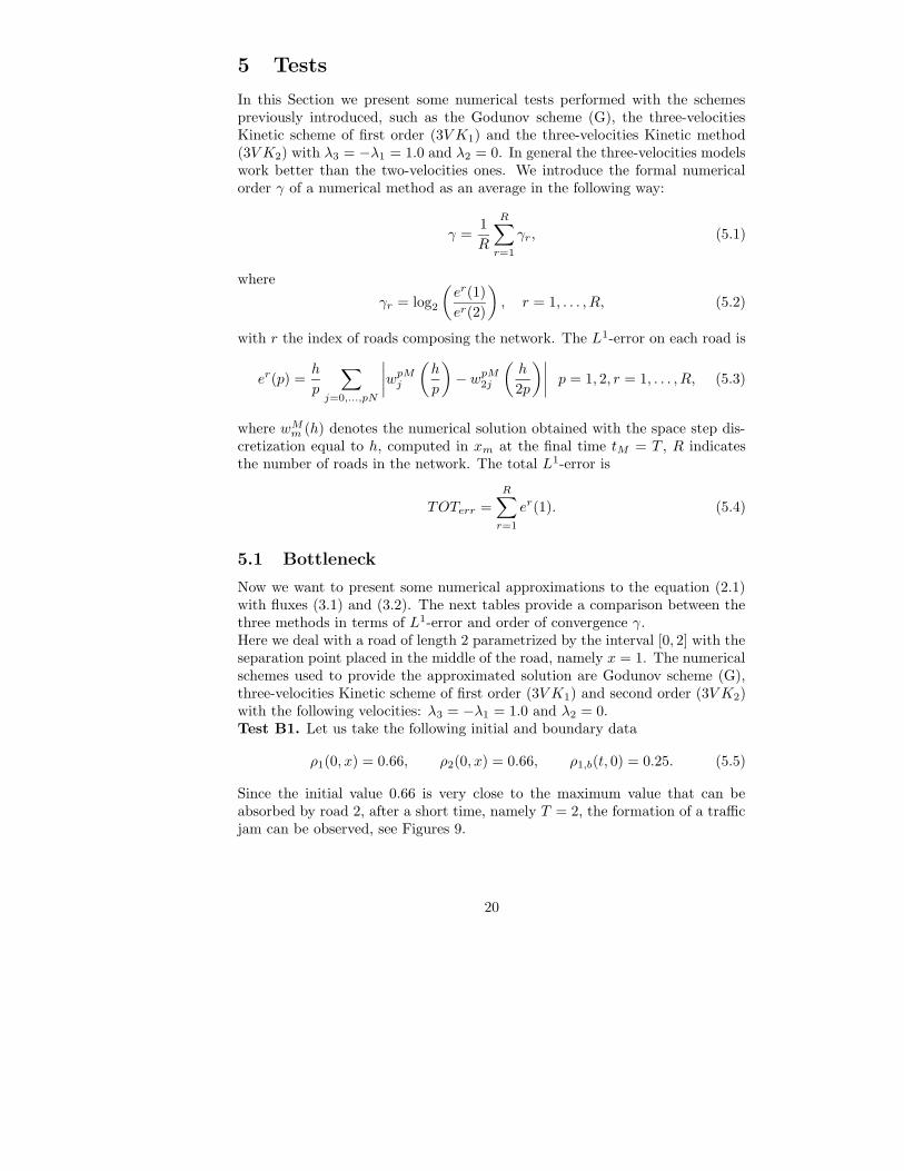
5 Tests

In this Section we present some numerical tests performed with the schemespreviously introduced, such as the Godunov scheme (G), the three-velocitiesKinetic scheme of first order (3V K1) and the three-velocities Kinetic method(3V K2) with λ3 = −λ1 = 1.0 and λ2 = 0. In general the three-velocities modelswork better than the two-velocities ones. We introduce the formal numericalorder γ of a numerical method as an average in the following way:

γ =1

R

R∑

r=1

γr, (5.1)

where

γr = log2

(er(1)

er(2)

), r = 1, . . . , R, (5.2)

with r the index of roads composing the network. The L1-error on each road is

er(p) =h

p

∑

j=0,...,pN

∣∣∣∣wpMj

(h

p

)− wpM2j

(h

2p

)∣∣∣∣ p = 1, 2, r = 1, . . . , R, (5.3)

where wMm (h) denotes the numerical solution obtained with the space step dis-cretization equal to h, computed in xm at the final time tM = T , R indicatesthe number of roads in the network. The total L1-error is

TOTerr =

R∑

r=1

er(1). (5.4)

5.1 Bottleneck

Now we want to present some numerical approximations to the equation (2.1)with fluxes (3.1) and (3.2). The next tables provide a comparison between thethree methods in terms of L1-error and order of convergence γ.Here we deal with a road of length 2 parametrized by the interval [0, 2] with theseparation point placed in the middle of the road, namely x = 1. The numericalschemes used to provide the approximated solution are Godunov scheme (G),three-velocities Kinetic scheme of first order (3V K1) and second order (3V K2)with the following velocities: λ3 = −λ1 = 1.0 and λ2 = 0.Test B1. Let us take the following initial and boundary data

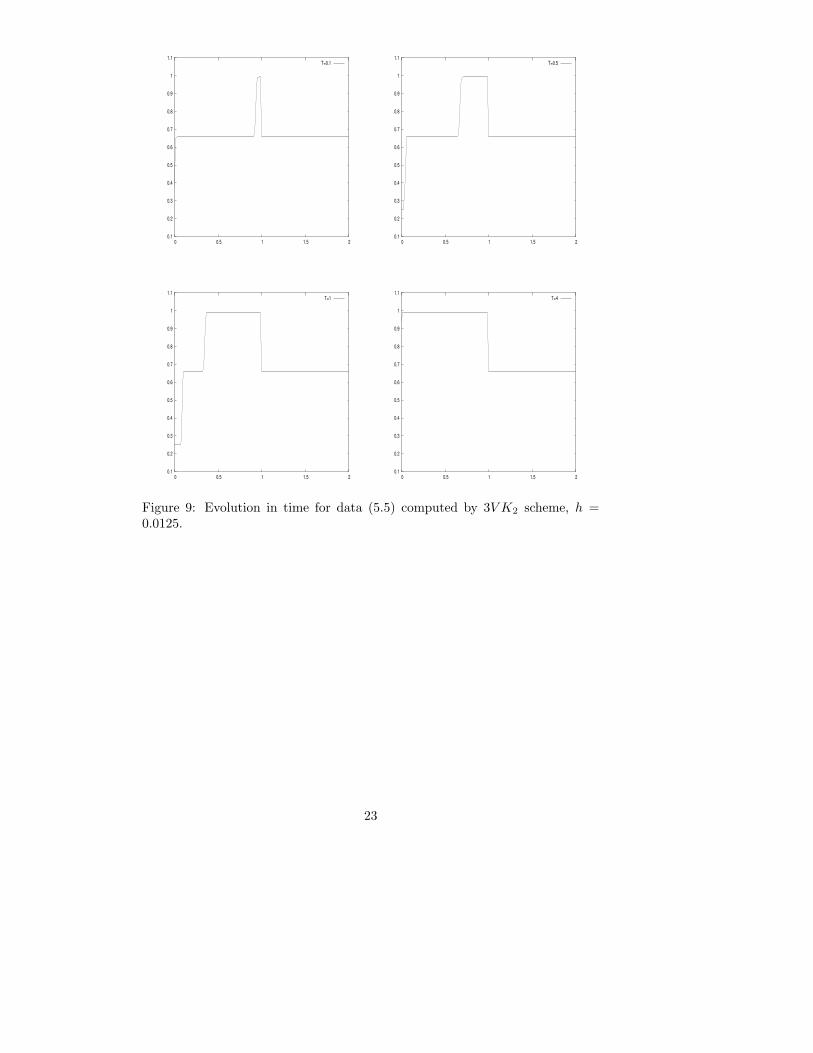
ρ1(0, x) = 0.66, ρ2(0, x) = 0.66, ρ1,b(t, 0) = 0.25. (5.5)

Since the initial value 0.66 is very close to the maximum value that can beabsorbed by road 2, after a short time, namely T = 2, the formation of a trafficjam can be observed, see Figures 9.

20

G 3V K1 3V K2

h γ L1 Error γ L1 Error γ L1 Error0.1 1.51554 3.347e-002 1.14981 2.886e-002 1.19519 2.931e-0020.05 0.89752 1.170e-002 0.83645 1.301e-002 0.92098 1.280e-0020.025 0.58367 6.285e-003 0.85088 7.284e-003 0.75549 6.761e-0030.0125 1.22648 4.194e-003 1.16427 4.038e-003 1.29260 4.005e-0030.00625 0.65763 1.792e-003 0.83753 1.802e-003 0.73386 1.635e-0030.003125 1.50268 1.136e-003 1.12176 1.008e-003 1.50429 9.830e-004

Table B1-1: Orders and errors of the approximation schemes Godunov (G), Kinetic

of first order (3V K1) and of second order (3V K2) for data (5.5), T = 0.5.

G 3V K1 3V K2

h L1 Error L1 Error L1 Error0.1 2.07651e-002 2.19038e-002 2.41712e-0020.05 1.25376e-002 1.45365e-002 1.35243e-0020.025 8.38778e-003 8.07708e-003 8.00970e-0030.0125 3.58458e-003 3.60392e-003 3.26967e-0030.00625 2.27234e-003 2.01675e-003 1.96603e-0030.003125 8.01899e-004 9.26764e-004 8.49835e-004

Table B1-2: Errors of the approximation schemes Godunov (G), Kinetic of first order

(3V K1) and of second order (3V K2) for data (5.5), T = 1.0.

21

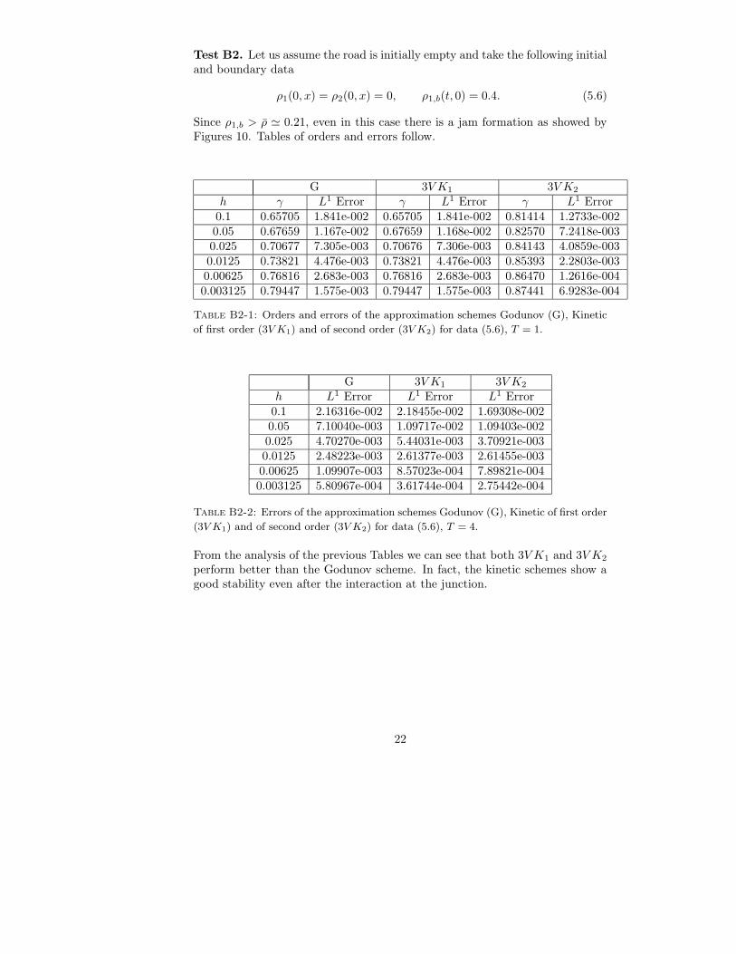
Test B2. Let us assume the road is initially empty and take the following initialand boundary data

ρ1(0, x) = ρ2(0, x) = 0, ρ1,b(t, 0) = 0.4. (5.6)

Since ρ1,b > ρ ' 0.21, even in this case there is a jam formation as showed byFigures 10. Tables of orders and errors follow.

G 3V K1 3V K2


Table B2-1: Orders and errors of the approximation schemes Godunov (G), Kinetic

of first order (3V K1) and of second order (3V K2) for data (5.6), T = 1.

G 3V K1 3V K2


Table B2-2: Errors of the approximation schemes Godunov (G), Kinetic of first order

(3V K1) and of second order (3V K2) for data (5.6), T = 4.

From the analysis of the previous Tables we can see that both 3V K1 and 3V K2

perform better than the Godunov scheme. In fact, the kinetic schemes show agood stability even after the interaction at the junction.

22

0.1

0.2

0.3

0.4

0.5

0.6

0.7

0.8

0.9

1

1.1

0 0.5 1 1.5 2

T=0.1

0.1

0.2

0.3

0.4

0.5

0.6

0.7

0.8

0.9

1

1.1

0 0.5 1 1.5 2

T=0.5

0.1

0.2

0.3

0.4

0.5

0.6

0.7

0.8

0.9

1

1.1

0 0.5 1 1.5 2

T=1

0.1

0.2

0.3

0.4

0.5

0.6

0.7

0.8

0.9

1

1.1

0 0.5 1 1.5 2

T=4

Figure 9: Evolution in time for data (5.5) computed by 3V K2 scheme, h =0.0125.

23

0.1

0.2

0.3

0.4

0.5

0.6

0.7

0.8

0.9

0 0.5 1 1.5 2

T=0.1

0.1

0.2

0.3

0.4

0.5

0.6

0.7

0.8

0.9

0 0.5 1 1.5 2

T=2

0.1

0.2

0.3

0.4

0.5

0.6

0.7

0.8

0.9

0 0.5 1 1.5 2

T=4

0.1

0.2

0.3

0.4

0.5

0.6

0.7

0.8

0.9

0 0.5 1 1.5 2

T=10

Figure 10: Evolution in time for data (5.6) computed by 3V K2 scheme, h =0.0125.

24

5.2 Two incoming - two outgoing roads

Recall definitions of Section 3 of junction J with two incoming roads and twooutgoing roads all parametrized with the interval [0, 1]. Here we refer to thesituation described in Appendix of [8], where the coefficients of the distributionmatrix A are such that 0 < α32 < α31 < 1/2. We set

α31 = α1, α32 = α2, α41 = 1− α1, α42 = 1− α2

and we introduce the notation

ρ1(0, x) = ρ1,0, ρ2(0, x) = ρ2,0, ρ3(0, x) = ρ3,0, ρ4(0, x) = ρ4,0.

The distribution matrix is fixed as

A =

(0.4 0.30.6 0.7

)(5.7)

and we consider the following constant initial and boundary data

ρ1,0 = ρ4,0 = σ, ρ2,0 = ρ3,0 = f−1

(α1

1− α2f(σ)

)= 0.82732683535,

ρ1,b(0, t) = σ, ρ2,b(0, t) = f−1

(α1

1− α2f(σ)

)= 0.82732683535 . (5.8)

Remark 5.1 Notice that the boundary condition is imposed only on the incom-ing roads, as for the outgoing ones we use a Neumann condition at the finalendpoint.

Let us introduce a perturbation on the initial data of road 1

ρ1(0, x) =

ρ1,0 = σ if 0 ≤ x ≤ 0.5,ρ1 if x ≥ 0.5,

(5.9)

and ρ1, ρ1,0, ρ2,0, ρ3,0, ρ4,0 be constants such that

σ < ρ2,0 < 1, σ < ρ3,0 < 1, ρ1 < σ, ρ1,0 = ρ4,0 = σ, (5.10)

f(ρ1,0) = f(ρ4,0) = f(σ), f(ρ2,0) = f(ρ3,0) =α1

1− α2f(σ),

so that (ρ1,0, ρ2,0, ρ3,0, ρ4,0) is an equilibrium configuration.In (5.9) assume to have a small perturbation represented by ρ1 = 0.4 and let theboundary data on road 1 be ρ1,b = 0.4. The initial data on other roads of thejunction, namely ρ2,0, ρ3,0, ρ4,0, are taken as in (5.8) and the boundary dataon road 2 is ρ1,b = ρ20. After a certain time (t ∼ 8) the wave (ρ1, ρ1,0) interactswith the junction thus determining a shock wave travelling on road 3. At timeT = 470 a new equilibrium configuration is reached: the value of density onroad 4 remains constant and on road 2 the final density is very close the initial

25

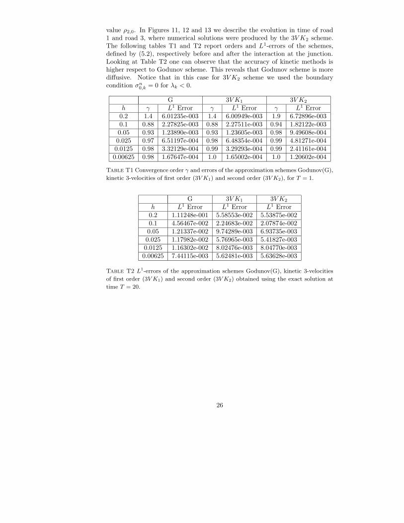
value ρ2,0. In Figures 11, 12 and 13 we describe the evolution in time of road1 and road 3, where numerical solutions were produced by the 3V K2 scheme.The following tables T1 and T2 report orders and L1-errors of the schemes,defined by (5.2), respectively before and after the interaction at the junction.Looking at Table T2 one can observe that the accuracy of kinetic methods ishigher respect to Godunov scheme. This reveals that Godunov scheme is morediffusive. Notice that in this case for 3V K2 scheme we used the boundarycondition σn0,k = 0 for λk < 0.

G 3V K1 3V K2


Table T1 Convergence order γ and errors of the approximation schemes Godunov(G),

kinetic 3-velocities of first order (3V K1) and second order (3V K2), for T = 1.

G 3V K1 3V K2


Table T2 L1-errors of the approximation schemes Godunov(G), kinetic 3-velocities

of first order (3V K1) and second order (3V K2) obtained using the exact solution at

time T = 20.

26

0.1

0.2

0.3

0.4

0.5

0.6

0.7

0.8

0.9

0 0.2 0.4 0.6 0.8 1

ROAD 1

0.1

0.2

0.3

0.4

0.5

0.6

0.7

0.8

0.9

0 0.2 0.4 0.6 0.8 1

ROAD 3

Figure 11: Initial configuration of data (5.9) with ρ1 = 0.4 = ρ1,b at time T = 0,with h = 0.025.

0.1

0.2

0.3

0.4

0.5

0.6

0.7

0.8

0.9

0 0.2 0.4 0.6 0.8 1

ROAD 1

0.1

0.2

0.3

0.4

0.5

0.6

0.7

0.8

0.9

0 0.2 0.4 0.6 0.8 1

ROAD 3

Figure 12: Situation after the interaction, T = 25, h = 0.025.

5.3 Traffic circles

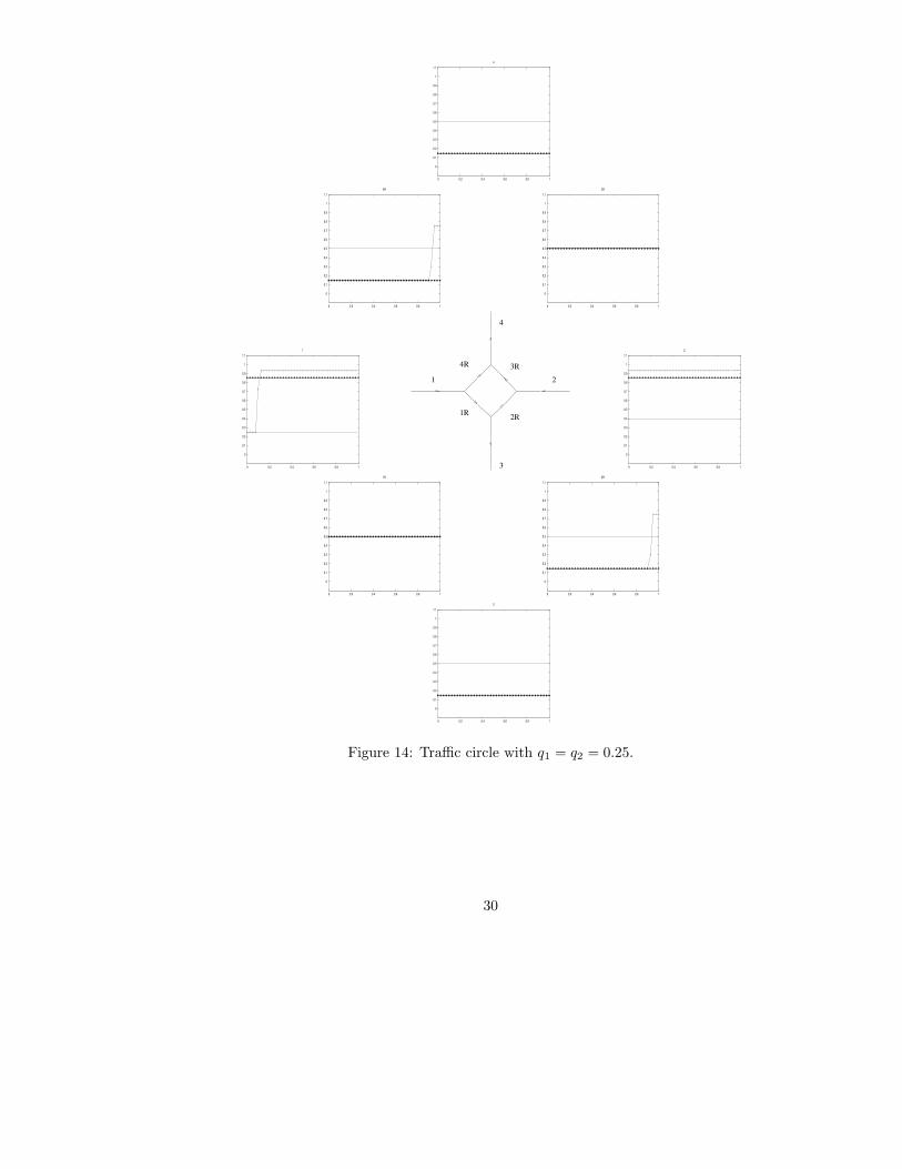
In the next pages we present some simulations reproducing a simple trafficcircle composed by 8 roads and 4 junctions. The numerical solutions have beengenerated by the 3V K2 method for h = 0.025 and cfl = 0.5.Consider the following initial and boundary data

ρ1(0, x) = 0.25, ρ2(0, x) = 0.4, ρ3(0, x) = 0.5, ρ4(0, x) = 0.5, (5.11)

ρ1R(0, x) = 0.5, ρ2R(0, x) = 0.5, ρ3R(0, x) = 0.5, ρ4R(0, x) = 0.5,

ρ1,b(t, 0) = 0.25, ρ2,b(t, 0) = 0.4 .

The distribution coefficients, namely (α1R,3, α1R,2R, α3R,4, α3R,4R), are assumed

27

0.1

0.2

0.3

0.4

0.5

0.6

0.7

0.8

0.9

0 0.2 0.4 0.6 0.8 1

ROAD 1

0.1

0.2

0.3

0.4

0.5

0.6

0.7

0.8

0.9

0 0.2 0.4 0.6 0.8 1

ROAD 3

Figure 13: Final configuration, T = 470, h = 0.025.

to be constant and are all equal to α = 0.5. Let us choose the following priorityparameters, which are q1 = q(1, 4R, 1R) = 0.25, q2 = q(2, 2R, 3R) = 0.25. Thefixed values imply that road 4R is the through street respect to road 1 and road2R is the through street respect to 1. The evolution in time of traffic is reportedin the next Figures 14. Observe that at time t = 5 shocks are generated on theentering roads 1 and 2, while rarefaction waves in the direction of traffic arecreated on roads 4R, 2R, 3, 4. Roads 1R and 3R do not change the level of thedensity. At t = 10 rarefaction waves travelling in the sense of traffic produce adecrease in the car density on roads 4R, 3R, 3, 4. On entering roads 1 and 2the effect of shocks travelling backwards is a considerable increase of the densityand, again, roads 1R and 3R have the same configuration, which correspondsto the maximum flux. At time T = 40 the roads entering in the circle have anhigh value of density as they wait at the junctions, while densities of roads inthe circle are lowered due to the fact that traffic is flowing towards the outgoingroads 3 and 4. We can observe that starting from the same configuration (5.11)but setting differently the right of way parameters, traffic within the circle isfluid and is distributed between the outgoing roads.Fig. 15, obtained for data (5.11) and q1 = q2 = 0.5, shows a situation quitesimilar to that in Fig. 14. The difference is represented by the values of densityon the roads 2R and 4R that reveal a shock formation with zero speed. As aconsequence, the time for covering the path of the circle from road 1 to road 4is higher than in the case depicted in Fig. 14. In particular, let δ be the portionof road 2R at the lowest value of density, i.e. 0.15, and 1− δ the other portionof the same road, we can estimate the time for covering the path from road 1to road 4. In the first case is

1

0.5+

1

0.85+

1

0.5∼ 5.17

28

while here (with δ = 0.5) we get

1

0.5+

δ

0.85+

1− δ0.15

+1

0.5∼ 7.92

and the difference between the previous and the current case is

∆t =1− δ0.15

− 1− δ0.85

= (1− δ)80

17,

that is greater as δ → 0.Let us set the right of way parameters as q1 = q(1, 4R, 1R) = 0.75, q2 =q(2, 2R, 3R) = 0.75. This means that road 1 is the through street respectto road 4R and road 2 is the through street respect to 2R. As before, thedistribution coefficients are assumed to be constant and all equal to α = 0.5.The evolution in time of traffic densities is described in Figure 16. One canobserve that at time t = 1.5 the chosen right of way parameters provoke shockspropagating backwards along roads 2R and 4R and consequently a shock iscreated on road 2. Successively, the density on roads 4R, 2R increases andshocks are propagating backwards on roads 1R and 3R. Roads 3 and 4 show avery low density of cars. At T = 40 densities on the incoming roads and withinthe circle (all equal to the maximum value ρmax = 1), represent a situation oftraffic jam, the so called bumper-to-bumper traffic. This means that no carscan exit the circle, as showed by the fact that roads 3 and 4 are empty. Hence,in that case, the choice of the right of way parameter determines a situation ofcompletely blocked traffic.In the next pages, Figures 16, 14, 15 show the evolution in time of the densityfor the discussed cases with the following legend:

Legend

t = 0

t = 40

t = 10

t = 5

29

0

0.1

0.2

0.3

0.4

0.5

0.6

0.7

0.8

0.9

1

1.1

0 0.2 0.4 0.6 0.8 1

4

0

0.1

0.2

0.3

0.4

0.5

0.6

0.7

0.8

0.9

1

1.1

0 0.2 0.4 0.6 0.8 1

4R

0

0.1

0.2

0.3

0.4

0.5

0.6

0.7

0.8

0.9

1

1.1

0 0.2 0.4 0.6 0.8 1

3R

0

0.1

0.2

0.3

0.4

0.5

0.6

0.7

0.8

0.9

1

1.1

0 0.2 0.4 0.6 0.8 1

1

1 2

1R 2R

3R4R

3

4

0

0.1

0.2

0.3

0.4

0.5

0.6

0.7

0.8

0.9

1

1.1

0 0.2 0.4 0.6 0.8 1

2

0

0.1

0.2

0.3

0.4

0.5

0.6

0.7

0.8

0.9

1

1.1

0 0.2 0.4 0.6 0.8 1

1R

0

0.1

0.2

0.3

0.4

0.5

0.6

0.7

0.8

0.9

1

1.1

0 0.2 0.4 0.6 0.8 1

2R

0

0.1

0.2

0.3

0.4

0.5

0.6

0.7

0.8

0.9

1

1.1

0 0.2 0.4 0.6 0.8 1

3

Figure 14: Traffic circle with q1 = q2 = 0.25.

30

0

0.1

0.2

0.3

0.4

0.5

0.6

0.7

0.8

0.9

1

1.1

0 0.2 0.4 0.6 0.8 1

4

0

0.1

0.2

0.3

0.4

0.5

0.6

0.7

0.8

0.9

1

1.1

0 0.2 0.4 0.6 0.8 1

4R

0

0.1

0.2

0.3

0.4

0.5

0.6

0.7

0.8

0.9

1

1.1

0 0.2 0.4 0.6 0.8 1

3R

0

0.1

0.2

0.3

0.4

0.5

0.6

0.7

0.8

0.9

1

1.1

0 0.2 0.4 0.6 0.8 1

1

1 2

1R 2R

3R4R

3

4

0

0.1

0.2

0.3

0.4

0.5

0.6

0.7

0.8

0.9

1

1.1

0 0.2 0.4 0.6 0.8 1

2

0

0.1

0.2

0.3

0.4

0.5

0.6

0.7

0.8

0.9

1

1.1

0 0.2 0.4 0.6 0.8 1

1R

0

0.1

0.2

0.3

0.4

0.5

0.6

0.7

0.8

0.9

1

1.1

0 0.2 0.4 0.6 0.8 1

2R

0

0.1

0.2

0.3

0.4

0.5

0.6

0.7

0.8

0.9

1

1.1

0 0.2 0.4 0.6 0.8 1

3


31

0

0.1

0.2

0.3

0.4

0.5

0.6

0.7

0.8

0.9

1

1.1

0 0.2 0.4 0.6 0.8 1

4

0

0.1

0.2

0.3

0.4

0.5

0.6

0.7

0.8

0.9

1

1.1

0 0.2 0.4 0.6 0.8 1

4R

0

0.1

0.2

0.3

0.4

0.5

0.6

0.7

0.8

0.9

1

1.1

0 0.2 0.4 0.6 0.8 1

3R

0

0.1

0.2

0.3

0.4

0.5

0.6

0.7

0.8

0.9

1

1.1

0 0.2 0.4 0.6 0.8 1

1

1 2

1R 2R

3R4R

3

4

0

0.1

0.2

0.3

0.4

0.5

0.6

0.7

0.8

0.9

1

1.1

0 0.2 0.4 0.6 0.8 1

2

0

0.1

0.2

0.3

0.4

0.5

0.6

0.7

0.8

0.9

1

1.1

0 0.2 0.4 0.6 0.8 1

1R

0

0.1

0.2

0.3

0.4

0.5

0.6

0.7

0.8

0.9

1

1.1

0 0.2 0.4 0.6 0.8 1

2R

0

0.1

0.2

0.3

0.4

0.5

0.6

0.7

0.8

0.9

1

1.1

0 0.2 0.4 0.6 0.8 1

3


32

In the same framework, we can also treat portions of urban network. In partic-ular, some simulations were carried out on a crucial area for traffic in the cityof Rome, which is represented by the Square of “Re di Roma”, in Fig. 17.

Figure 17: Re di Roma.

For some animations, see [6].

6 Conclusions

An elaboration and an implementation of Godunov method and of kineticschemes even extended to second order provided numerical solutions to theproblem of traffic flows on road networks. Since along the roads the schemespresent the same features as for conservation laws, the new and original aspectis given by the treatment of the solution at junctions. Our tests show the ef-fectiveness of the approximations, revealing that kinetic schemes of 3-velocitiesare more accurate than Godunov scheme.

Acknowledgments. The authors would like to thank Antonino Sgalambrofor his assistance with the computational work.

33

References

[1] D. Aregba-Driollet, V. Milisic, Kinetic Approximation of a Boundary ValueProblem for Conservation Laws, Numerische Mathematik 97 (2004), pp.595-633.

[2] V. Astarita, Node and Link Models for Network Traffic Flow Simulation,Mathematical and Computer Modelling 35 (2002), pp. 643-656.

[3] D. Aregba-Driollet, R. Natalini, Discrete Kinetic Schemes for Multidimen-sional Systems of Conservation Laws, SIAM J. Numer. Anal. 37 (2000),No. 6, pp. 1973-2004.

[4] C. Bardos, A. Y. Le Roux, J. C. Nedelec, First Order Quasilinear Equationwith Boundary Conditions, Commun. Partial Differential Equations, 4(1979), pp. 1017-1034.

[5] A. Bressan, Hyperbolic systems of conservation laws. The one-dimensionalCauchy problem. Oxford Lecture Series in Mathematics and its Appli-cations. 20. Oxford University Press (2000).

[6] G. Bretti, A. Sgalambro,http://www.iac.rm.cnr.it/∼bretti/TrafficNumericalSolution.html .

[7] Y. Chitour, B. Piccoli, Traffic circles and timing of traffic lights for carsflow, Discrete and Continuous Dynamical Systems-Series B (to appear).

[8] G. M. Coclite, M. Garavello, B. Piccoli, Traffic Flow on a Road Network,Siam Math. Anal. (to appear).

[9] C.M. Dafermos, Hyperbolic conservation laws in continuum physics.Grundlehren der Mathematischen Wissenschaften. 325. Berlin: Springer(2000).

[10] S.K. Godunov, A finite difference method for the numerical computationof discontinuous solutions of the equations of fluid dynamics, Mat. Sb.47, 1959, pp. 271-290.

[11] E. Godlewski, P.A. Raviart, Hyperbolic systems of conservation laws,Mathematiques & Applications [Mathematics and Applications], 3/4.Ellipses, Paris (1991).

[12] R. Haberman, Mathematical models, Prentice-Hall, Inc. New Jersey, 1977,pp. 255-394.

[13] H. Holden and N. H. Risebro, A Mathematical Model of Traffic Flow on aNetwork of Unidirectional Roads, SIAM J. Math. Anal., 26 (1995), pp.999-1017.

[14] A. Klar, Kinetic and macroscopic traffic flow models, Lecture notes for theXX School of Computational Mathematics, ”Computational aspects inkinetic models”, Piano di Sorrento (Italy) September 22-28, 2002.

[15] R.J. Leveque, Finite volume methods for hyperbolic problems. CambridgeTexts in Applied Mathematics. Cambridge University Press (2002).

34

[16] M. J. Lighthill, G. B. Whitham, On kinematic waves. II. A theory of traf-fic flow on long crowded roads. Proc. Roy. Soc. London. Ser. A., 229(1955), pp. 317–345.

[17] R. Natalini, A Discrete Kinetic Approximation of Entropy Solutions to Mul-tidimensional Scalar Conservation Laws, Journal of differential equa-tions, 148 (1998), pp. 292-317.

[18] P. I. Richards, Shock Waves on the Highway, Oper. Res., 4 (1956), pp.42–51.

[19] G.B. Whitham, Linear and nonlinear waves. Pure and Applied Mathemat-ics. A Wiley-Interscience Series of Texts, Monographs, and Tracts. NewYork etc.: John Wiley & Sons. (1974).

35

Documents

Numerical Approximations of a Tra c Flow Model on Networks