Embed Size (px)
Citation preview

NUMERICAL AND EXPERIMENTAL STUDIES
OF WOOD SHEATHED COLD-FORMED STEEL FRAMED SHEAR WALLS
by
Hung Huy Ngo
A thesis submitted to Johns Hopkins University in conformity with the requirements for the
degree of Master of Science in Engineering
Baltimore, Maryland
August, 2014
© 2014 Hung Huy Ngo
All Rights Reserved

ii
Abstract
This thesis presents phase one of a project with the objective of exploring the impact of
non-conventional detailing of wood-sheathed, cold-formed steel (CFS) framed, shear
walls. The work shown herein includes the development and validation of a high fidelity
shell finite element model and the preparation for future full-scale shear wall testing.
Current design of wood sheathed CFS framed shear walls relies on deformations and
associated ductility at the frame-to-sheathing connections (see e.g. AISI S213-12).
Prescriptive requirements and capacity-based design principles are utilized to insure the
desired limit state. Reliability of this complex subsystem has not formally been evaluated
based on the potential limit states. Further, the desire for connections to be the controlling
limit state is contrary to general design, where connection reliability employs a higher
reliability index β (typically 3.5) than member reliability (β typically 2.5). A high fidelity
shell finite element model is developed in ABAQUS for prediction of lateral response of
wood-sheathed CFS framed shear walls. CFS members and sheathing panels are modeled
with shell elements, sheathing-to-frame fasteners are modeled with nonlinear spring
elements, and hold-downs are modeled as bi-linear springs. The walls are subjected to
either monotonic or cyclic (CUREE protocol) lateral loading by displacement-based
analysis. The model is validated against available testing and is demonstrated to be able
to recreate the full-scale tests. Along with the numerical study, the preparation for future
full-scale shear wall tests including the design of testing rig, development of sensor plan,
material tensile testing, and assembly of preliminary test specimen were also conducted.
Phase two of the project, which involves the parametric study of various unconventional

iii
shear walls using the developed modeling protocol and non-conventional full-scale shear
wall testing, is now underway.
Advisor: Benjamin Schafer, Professor and Chair
Department of Civil Engineering, Johns Hopkins University

iv
Table of Contents
Abstract .............................................................................................................................. ii
Acknowledgments ............................................................................................................ vi
Chapter 1 - Introduction .................................................................................................. 1
1.1. Cold-Formed Steel Structures .......................................................................................... 1
1.2. Cold-Formed Steel Shear Walls ........................................................................................ 1
1.3. Purpose and Scope of Research ....................................................................................... 2
1.4. Thesis Organization .......................................................................................................... 3
Chapter 2 - Previous Research on Wood Sheathed Cold-Formed Steel Shear Walls 5
2.1. Previous Testing ............................................................................................................... 5
2.2. Computational Modeling ................................................................................................. 6
2.3. CFS-NEES Shear Wall Full-Scale Testing .......................................................................... 7
Chapter 3 - High Fidelity Computational Modeling ................................................... 14
3.1. Introduction ................................................................................................................... 14
3.2. General Model Details ................................................................................................... 15
3.3. Element and Mesh Discretization .................................................................................. 16
3.4. Material Properties ........................................................................................................ 18
3.5. Out-of-Plane Support ..................................................................................................... 18
3.6. Anchor Bolt .................................................................................................................... 19
3.7. Hold-Down ..................................................................................................................... 20
3.8. Steel-to-Steel Connection .............................................................................................. 21
3.9. Sheathing-to-Frame Connections .................................................................................. 23
3.10. Loading Model ........................................................................................................... 24
Chapter 4 - Computational Results and Discussion .................................................... 26
4.1. Force-Displacement Response ....................................................................................... 26
4.2. Sheathing-to-Frame Connection Failure ........................................................................ 30
4.3. Deformation of Cold-Formed Steel Frame Members .................................................... 33
4.4. Summary ........................................................................................................................ 36
Chapter 5 - Experimental Setup .................................................................................... 37
5.1. Testing Rig ...................................................................................................................... 37
5.2. Instrumentation Plan ..................................................................................................... 41

v
5.3. Load Protocol ................................................................................................................. 43
5.4. Typical Test Specimen .................................................................................................... 43
5.5. Material Properties ........................................................................................................ 45
Chapter 6 - Future Work ............................................................................................... 46
Chapter 7 - Conclusions ................................................................................................. 47
Appendix A - Deformed Shape Of Computational Models ........................................ 49
Appendix B - AutoCAD Drawings ................................................................................ 55
References ........................................................................................................................ 63
Curriculum Vitae ............................................................................................................ 66

vi
Acknowledgments
First, I would like to thank my advisor, Professor Benjamin Schafer for all of his help and
guidance throughout my research. His passion and love for cold-formed steel has been
strongly inspiring me.
I would also like to express my gratitude to Professor Lori Graham-Brady for her help
with the preparation of this thesis.
Special thanks are also given to all of my colleagues in Professor Schafer's Thin-Walled
Structures group for creating an inspirational and supportive research environment.
Utmost appreciation is extended to Dr. Shahabeddin Torabian for his enormous help with
my computational modeling and experimental setup.
Lastly, I want to sincerely thank my family and friends who have always unconditionally
supported me throughout my life journey.

1
Chapter 1 - Introduction
1.1. Cold-Formed Steel Structures
Cold-formed steel (CFS) is commonly known as the steel products made by rolling or
pressing thin steel sheet into goods at room temperature. This type of steel product has
become more and more popular since the publication of first AISI Specification for the
Design of Cold Formed Steel Structural Members in1946. Cold-formed steel members
have been mostly used in residential and industrial buildings, bridges, storage racks, and
others.
The source for the rapidly growing interest in using cold-formed steel is the advantages
of this material over other construction materials. Two main advantages are light weight
and the ease in construction. However, being well known for the large width-to-thickness
ratio due to small thickness, cold-formed steel members are prone to instability problems.
In addition to global buckling, local and distortional buckling are often observed in cold-
formed steel sections.
1.2. Cold-Formed Steel Shear Walls
Shear wall has been known as the primary lateral force resisting system for cold-formed
steel framing. There are many types of cold-formed steel framed shear wall such as strap-
braced wall, knee-braced wall, corrugated wall, or walls sheathed with one or a
combination of sheathing, e.g. wood board, steel sheet, gypsum board or calcium silicate

2
board. This thesis will focus on the wood-sheathed cold-formed steel framed shear wall
which is the most common type of shear wall used in cold-formed steel construction.
As depicted in Figure 1.1, wood-sheathed cold-formed steel framed shear wall typically
consists of a cold-formed steel frame connected to oriented strand board (OSB) panels
with a series of fasteners, which are now called sheathing-to-frame connections. Current
design of wood-sheathed cold-formed steel framed shear wall is in accordance with the
American Iron and Steel Institution Lateral Design Standard (AISI S213-07) which relies
on deformations and associated ductility at these sheathing-to-frame connections.
Figure 1.1. Components of wood-sheathed cold-formed steel framed shear walls
1.3. Purpose and Scope of Research
As mentioned in previous section, current design of wood-sheathed cold-formed steel
framed shear wall is based on only the limit state of sheathing-to-frame connections. The
objective of the overall project, of which the research presented herein serves as the
initial phase, is to explore limit states other than those associated with the fastener in the

3
shear wall so that reliability of this complex subsystem can formally be evaluated based
on potential limit states. These non-traditional limit states consist of, but are not limited
to, chord stud buckling and hold-down failure.
The overall project consists of four main tasks as follows.
(a) Development of high fidelity computational modeling of wood-sheathed cold-
formed steel framed shear walls
(b) Preparation for future full-scale shear wall testing
(c) Parametric study of wood-sheathed cold-formed steel framed shear walls with
non-conventional detailing based on developed modeling protocol
(d) Full-scale testing on wood-sheathed cold-formed steel framed shear walls with
non-conventional detailing
The scope of the research detailed in this thesis is limited to (a) and (b) which is
considered as the first phase of the overall project.
1.4. Thesis Organization
The remainder of this thesis is organized in the following manner. Chapter 2, Previous
Research on Wood Sheathed Cold-Formed Steel Shear Walls, provides a review of recent
literature on wood sheathed cold-formed steel shear walls including experimental testing
and computational modeling. Chapter 3, High Fidelity Computational Modeling, presents
a reliable modeling protocol that can be used to accurately simulate a wood-sheathed
cold-formed steel shear wall using the Abaqus software. Chapter 4, Computational
Results and Discussion, provides the computational results of the nonlinear collapse

4
pushover analyses of the developed high fidelity finite element models and compares
with the experimental results. Chapter 5, Experimental Setup, details the experimental
setup for future full-scale shear wall tests. Chapter 6, Future Work, looks into the
research needs to be conducted in the future, i.e. phase two of the overall project. Chapter
7, Conclusions, summarizes the work presented in this thesis. The Appendices provide
the complete simulation results and drawings of the members designed for future shear
wall tests. The References provide the works and publications cited throughout this
thesis.

5
Chapter 2 - Previous Research on Wood Sheathed Cold-Formed Steel Shear Walls
A review of recent literature on wood sheathed cold-formed steel shear walls including
experimental testing and computational modeling is provided in this chapter. The test
program conducted by Liu et al. (2012a,b) as a part of National Science Foundation
(NSF) funded Network for Earthquake Engineering Simulation (CFS-NEES) project is
focused.
2.1. Previous Testing
As summarized in Branston et al. (2006), an extensive program of tests on light-gauge
steel-frame wood structural panel shear walls was conducted at McGill University with
the purpose of developing a shear wall design method to be used by engineers in Canada.
This test program involved 16 shear wall configurations with 109 specimens tested by
Boudreault et al. (2005), Branston et al.(2004), and Chen et al. (2004). These 16
configurations were based on the following main details: (i) wall height 2440 mm [96in.],
(ii) wall length 610, 1220, and 2440 mm [24, 48, and 96 in.], (iii) sheathing types
including Douglas-fir plywood (DFP), Canadian softwood plywood (CSP), and oriented
strand board (OSB) wood structural panels, (iv) 1.12 mm [44 mils] thick 230 MPa [33ksi]
grade steel framing members, (v) Simpson Strong-Tie S/HD10, and (vi) loading
protocols including monotonic, reversed cyclic Consortium of Universities for Research
in Earthquake Engineering (CUREE), and reversed cyclic Sequential Phased
Displacement (SPD). As described by Branston et al. (2006), in most instances, failure
occurs at the fasteners connecting the wood structural panel to the cold-formed steel
frame. The failure modes are the combinations of the following three basic modes: pull-

6
through of the screws in the wood sheathing, tearing out of the sheathing edge, and wood
bearing. A thorough evaluation of the structural performance of the tested shear walls,
given the variation in wall size, screw spacing, wood panel type, and load protocol is
provided by Chen et al. (2006).
A series of 16 tests on wood sheathed cold-formed steel shear walls was conducted by
Liu et al. (2012a,b) as a part of NSF sponsored CFS-NEES project. The objective of this
testing is to study the impact of practical details such as the use of ledger (rim track),
interior gypsum board, and low-grade small-thickness field stud on the shear wall's
structural behavior. A detailed description of this test series will be provided in Section
2.3 since the data obtained from this testing will be used to validate the modeling
protocol developed by the author as presented in Chapter 3.
2.2. Computational Modeling
An effort in simulating wood sheathed cold-formed steel shear walls is presented in
Buonopane et al. (2014). Fastener-based computational models were developed in
Opensees and validated against the testing conducted by Liu et al. (2012a,b). The
developed models used beam-column elements for the framing members and rigid
diaphragms for the sheathings. Each sheathing-to-frame fastener was modeled by means
of either a radially symmetric linear or non-linear spring element with parameters
determined from fastener tests. Pinching4 material model was incorporated to account for
the reloading/unloading behavior of sheathing-to-frame fastener under cyclic loading.
The impact of specific modeling features including hold-down, shear anchor, panel seam,
and ledger track on the shear wall's initial stiffness and lateral strength was investigated

7
and suggestions on the technique to simulate wood sheathed cold-formed steel shear
walls was provided. The development of these fastener-based computational models is
ongoing. It is important to note that Euler–Bernoulli beam theory is applied to the beam-
column element in Opensees that was used for modeling framing members. Therefore,
shear deformation is not taken into account because plane sections remain plane and
normal to the neutral axis after bending. In addition, due to the nature of beam-column
element, local and distortional buckling are not captured. A more advanced
computational modeling is required if the deformation of framing members needs to be
focused.
2.3. CFS-NEES Shear Wall Full-Scale Testing
The full-scale shear wall tests conducted by Liu et al. (2012a,b) was motivated by the
shear walls designed for a two-storey cold-formed steel ledger-framed building (Madsen
et al. 2011) that underwent full-scale shake table testing at University at Buffalo
(Peterman et al. 2014) as a part of CFS-NEES project. The details of this test series
including test setup, loading protocol, test specimens, material properties, and test results
are provided as follows.
Test setup
All of 16 tests were performed on an adaptable structural steel testing frame which is
equipped with one MTS 35 kip hydraulic actuator with 5 in. stroke. As depicted in
Figure 2.1 (a), a specimen is bolted to the rig via a steel base at the bottom and connected
to a structural WT at the top with two lines of self-drilling screws at every 3 in. along the
top track. This WT's role is to transfer lateral force from the actuator to the shear wall. A

8
series of rollers is employed to provide out-of-plane support at the top of the specimen as
shown in Figure 2.1 (c). Five position transducers are placed following the sensor plan
provided in Figure 2.1 (b) to measure deflection of the shear wall in the north, south, and
lateral directions.
(a) (b)
(c)
Figure 2.1. CFS-NEES shear wall test setup (a) testing rig with 4 ft × 9 ft specimen, (b) sensor plan, (c) out-of-
plane support (Liu et al. 2012a,b)
SO
UT
H
NO
RT
H
Load
5
1
3
4
6

9
Loading protocol
Both monotonic and cyclic tests were conducted using displacement control. Monotonic
loading procedure is in accordance with ASTM E564(Standard Practice for Static Load
Test for Shear Resistance of Framed Walls Buildings). Cyclic loading follows the
CUREE protocol which is in accordance with the test method C in ASTM E2126. The
utilized CUREE loading procedure with a frequency of 0.2 Hz is provided in Figure 2.2.
Figure 2.2. CUREE loading history
Test specimens
Test matrix is provided in Table 2.1. 16 shear wall configurations differ in wall size, load
type, grade and thickness of field stud, location of seam on OSB, sheathing type, and
whether or not ledger is present. The baseline specimen consists of either 4 ft × 9 ft or 8 ft
0 50 100 150 200 250-200
-150
-100
-50
0
50
100
150
200
Time(s)
Specim
en d
ispla
cem
ent(
%
)
CUREE protocol

10
× 9 ft cold-formed steel frame sheathed with either oriented strand board (OSB) or
gypsum board or both. As depicted in Figure 2.3 (a)-(b), the frame is assembled with
600S162-54 (50ksi) studs connected to two 600T150-54 (50ksi) tracks with No. 10
flathead screws. Studs are spaced at 24 in. on center and braced with a 1.5 in. ×54mil
cold rolled channel (CRC) as shown in Figure 2.3 (d). Chord studs consist of two studs
connected back-to-back to each other with pairs of No. 10 flathead screws spaced every
12 inches. 1200T200-097 (50ksi) track is used for the ledger when ledger is present.
Simpson Strong-Tie S/HDU6 hold downs are attached on the inward face at the bottom
of the chord studs as shown in Figure 2.3 (e). The OSB used as sheathing in the test is
7/16 in., 24/16 rated, exposure 1. The gypsum board is 4 ft wide and 8 ft tall with 0.5 in.
thickness. OSB board is connected to the frame with No. 8 flathead fasteners and No. 6
fasteners are used for attaching gypsum board. The layout of these fasteners for 4 ft × 9 ft
shear walls is provided in Figure 2.3 (a)-(b). The details are similar for 8 ft × 9 ft shear
walls. 1.5 in. wide 54 mil strap is employed at horizontal seam of OSB boards.
Table 2.1. Test matrix (Liu et al. 2012a)
Test Wall Size Load Type F. Sheathing B. Sheathing Stud Ledger H. Seam V. Seam Peak Load Peak Disp.
quantity mono/cyclic OSB Gypsum 600S162-xx 1200T200-97 P ave Δ ave
unit ftxft - ✔/- ✔/- 1/1000 in. ✔/- ft ft plf in
1c 4x9 Monotonic ✔ - 54 ✔ 8’up - 1225 2.96
2 4x9 Cyclic ✔ - 54 ✔ 8’up - 1102 2.82
3 4x9 Cyclic ✔ ✔ 54 ✔ 8’up - 1111 2.67
4 4x9 Cyclic ✔ - 54 - 8’up - 1004 2.40
5 4x9 Cyclic ✔ - 54 ✔ 7’up - 987 2.39
6 4x9 Cyclic ✔ - 54 - 7’up - 1031 2.24
7* 4x9 Cyclic ✔ - 54 - 8’up 1’over 897 2.23
8* 4x9 Cyclic ✔ - 54 - 8’up 2’over 982 3.33
9 4x9 Cyclic ✔ - 54 - 8’up 2’over 906 3.56
10 4x9 Cyclic ✔ - 54 - 4.5’up 2' over 950 2.94
11c 8x9 Monotonic ✔ - 54 ✔ 8’up - 1089 2.42
12 8x9 Cyclic ✔ - 54 ✔ 8’up - 1156 1.96
13 8x9 Cyclic ✔ ✔ 54 ✔ 8’up - 1232 1.91
14 8x9 Cyclic ✔ - 54 - 8’up - 1023 1.94
15 8x9 Cyclic ✔ - 33 - 8’up - 861 1.64
16 8x9 Cyclic - ✔ 54 ✔ 8’up - 231 1.47
Notes: CUREE protocol employed for cyclic testing, *additional field stud 1' over from side

11
(a) (b)
(c) (d)

12
(e)
Figure 2.3. Shear wall specimen (a) front view of 4 ft × 9 ft specimen, (b) back view of 4 ft × 9 ft specimen, (c)
ledger, (d) wall bracing, (e) hold-down (Peng et al. 2012a,b, Peterman et al. 2014)
Material properties
Coupon tests of the stud and track material were conducted according to the ASTM A370
(2006) “Standard Test Methods and Definitions for Mechanical Testing of Steel
Products.” A summary of the test results is provided in Table 2.2.
Table 2.2. Coupon test summary (Liu et al. 2012a)
Uncoated
thickness
Yield stress
Fy
Tensile
strength Fu
Fu/Fy
Elongation for 2 in.
gage length
(in.) (ksi) (ksi) (%)
54mil-50ksi stud 0.0566 56.1 78.8 1.4 14.90%
54mil-50ksi track 0.0583 64.3 72.4 1.13 16.50%
54mil-50ksi stud* 0.057 54.5 74.2 1.36 27.60%
33mil-33ksi stud 0.0365 51.5 59.9 1.16 18.00%
54mil-33ksi stud 0.0564 55.3 79.4 1.43 19.10%
97mil-50ksi ledger 0.1014 45.4 61.5 1.35 30.50%
Components
Note: 54mil-50ksi stud* is the second set of purchased studs which were used in all the 8ft x 9ft shear
walls as a field stud.

13
Test results
Table 2.3 provides a summary of the shear wall test results. In summary, failure typically
occurred at sheathing-to-frame connection locations. Practical details including ledger
track, interior gypsum board, panel seams, grade and thickness of field stud are
demonstrated to have a great impact on the specimens’ shear capacity. Finally, measured
capacity exceeded the nominal capacity specified in the design code AISI-S213-07.
Table 2.3. Summary of shear wall test results (Liu et al. 2012a)
Test Peak Load Lateral Deflection at Peak Avg. Load1
Avg. Disp2
Failure Mode3
quantity P+ P- Δ+ Δ- P ave Δ ave
unit plf plf in. in. plf in. -
1c 1225 - 2.96 - 1225 2.96 PT
2 1160 1044 2.92 2.71 1102 2.82 PT
3 1265 958 2.87 2.44 1111 2.67 PT
4 1046 963 2.88 1.93 1004 2.40 PT
5 1023 950 2.83 1.96 987 2.39 PT
6 1232 830 2.78 1.69 1031 2.24 PT
7* 876 918 2.55 1.91 897 2.23 PT
8* 1036 929 3.66 3.00 982 3.33 PT
9 921 890 4.20 2.92 906 3.56 PT
10 951 950 2.91 2.98 950 2.95 PT
11c 1089 - 2.42 - 1089 2.42 PT+B
12 1256 1055 2.27 1.66 1156 1.96 PT+B
13 1327 1138 2.20 1.62 1232 1.91 PT+B
14 1056 990 2.22 1.66 1023 1.94 PT+B
15 883 839 1.62 1.67 861 1.64 PT
16 259 202 1.22 1.73 231 1.47 PT1Average of P+ and P-,
2Average of Δ+ and Δ-,
3PT = fastener pull-through and B = fastener bearing
*Additional filed stud 1'over from side
14
Chapter 3 - High Fidelity Computational Modeling
3.1. Introduction
The ability to perform advanced computational modeling is essential for the development
of performance-based seismic design methods of cold-formed steel structures in general
and cold-formed steel shear walls in particular. This chapter presents a reliable modeling
protocol that can be used to accurately simulate a wood-sheathed cold-formed steel shear
wall using the Abaqus software. This modeling protocol will not only enable engineers to
predict the lateral capacity but also provide a thorough insight into the failure mechanism
of the wood-sheathed cold-formed steel shear wall subjected to lateral loading.
This modeling protocol is developed based on the effort of reproducing the full-scale
cold-formed steel shear wall tests conducted by Liu et al. (2012a,b) as summarized in
Chapter 2. Specifically, a series of ten high fidelity shell finite element models are
initiated in Abaqus to simulate ten shear wall specimens of which details are shown in
Table 3.1. Each of the following sections will describe the modeling of one or more
components in the specimen.
15
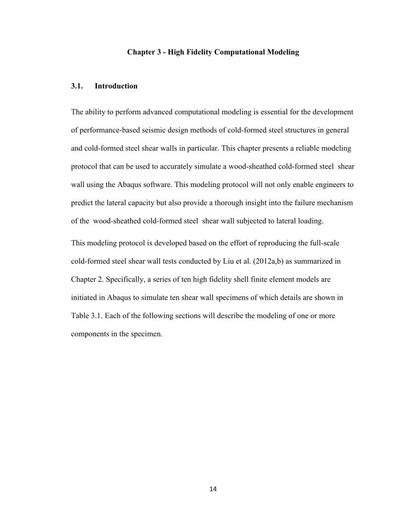
Table 3.1. Model matrix
3.2. General Model Details
Figure 3.1 shows the assembly of a 4ft×9ft and a 8ft×9ft shear wall in Abaqus. The
specimen geometry and practical details including the use of ledger (rim track), interior
gypsum board, and smaller thickness for field stud follow that of Liu et al. (2012a) as
summarized in Table 3.1 and Table 3.2. Herein, for all ten finite element models,
nonlinear collapse pushover analysis is conducted. Newton-Raphson numerical method is
used for solving nonlinear equations. In this research, seam on sheathing is ignored.
Geometric imperfections, residual stresses and strains are not included.
Table 3.2. General model details
Model Num. Test Num. Wall Size Load Type F. Sheathing B. Sheathing Stud Ledger
quantity mono/cyclic OSB Gypsum 600S162-xx 1200T200-97
unit ftxft - ✔/- ✔/- 1/1000 in. ✔/-
1 1c 4x9 Monotonic ✔ - 54 ✔
2 2 4x9 Cyclic ✔ - 54 ✔
3 3 4x9 Cyclic ✔ ✔ 54 ✔
4 4 4x9 Cyclic ✔ - 54 -
5 11c 8x9 Monotonic ✔ - 54 ✔
6 12 8x9 Cyclic ✔ - 54 ✔
7 13 8x9 Cyclic ✔ ✔ 54 ✔
8 14 8x9 Cyclic ✔ - 54 -
9 15 8x9 Cyclic ✔ - 33 -
10 16 8x9 Cyclic - ✔ 54 ✔
Notes: CUREE protocol employed for cyclic testing
Stud 600S162-54; 9ft
Track 600T150-54; 4ft or 8ft
OSB Panel 7/16" thick, 24/16 rated, exposure 1
Gypsum Panel 1/2" thick
Hold-Down S/HDU6

16
(a) (b)
Figure 3.1. Assembly of (a) 4ft×9ft and (b) 8ft×9ft shear wall in Abaqus
3.3. Element and Mesh Discretization
Cold-formed steel framing members and sheathing are modeled as four-node shell finite
elements S4R in Abaqus. This type of element uses linear shape functions and has
reduced integration scheme to prevent shear blocking in coarse mesh. Five integration
points are utilized through the thickness of the element. Schafer et al. (2010) studied the
sensitivity to element choice and mesh in the computational modeling of cold-formed
steel and demonstrated that the mesh density has a great impact on the response of cold-
formed steel members in finite element analysis. A coarse mesh can be adequate for
capturing the distortional and global buckling modes but cannot accurately reproduce
local buckling modes. On the other hand, a medium or fine mesh can represent all

17
buckling modes including local, distortional, and global with reasonable accuracy. In
addition, once a reasonable mesh is used, the difference in response between different
type of element becomes small. For these reasons, as depicted in Figure 3.2, a relatively
fine mesh is used in this modeling effort. A code is written in Matlab to generate the
mesh for the model with a seed size corresponding to 0.25 inch in real length used for
steel members and a seed size corresponding to 2 inches in real length used for
sheathing. This mesh discretization allows two elements on the lip of the stud so that
local buckling can be reproduced if occurs at these locations. Aspect ratio of the elements
is kept as close to one as practical and limited to be smaller than 2.5.
(a) Stud (b) Track
(c) Ledger (d) Sheathing
Figure 3.2. Shell finite element mesh of (a) stud, (b) track, (c) ledger, and (d) sheathing

18
3.4. Material Properties
As depicted in Table 3.3, cold-formed steel is modeled as isotropic elastic with Young's
modulus E=29,500ksi and Poisson's ratio v= 0.3. This value for Young's modulus
E=29,500ksi is commonly used in the computational modeling of cold-formed steel.
According to Abaqus analysis user's guide, this type of material is adequate since elastic
strains are expected to be small (less than 5%). Both sheathing material, oriented strand
board (OSB) and gypsum, are modeled as isotropic elastic with a large Young's modulus
E=30,000ksi and Poisson's ratio v= 0.3 to minimize diaphragm deformations.
Table 3.3. Material modeling
3.5. Out-of-Plane Support
The out-of-plane support of the top track in the experiments as described in Chapter 2
was included in the model as transverse roller constraints. As depicted in Figure 3.3, two
lines of nodes on the web of the top track at the exact location of the screws connecting
the top of shear wall specimen to the structural WT member are fixed in the transverse
direction. The purpose of this constraint is to restrict the shear wall to in-plane
movement.
Material Young's Modulus Poisson's ratio
Quantity E v
Unit (ksi)
Steel 29,500 0.3
OSB 30000* 0.3
Gypsum 30000* 0.3
* Rigid assumption

19
Figure 3.3. Modeling of out-of-plane support
3.6. Anchor Bolt
Figure 3.4 shows the modeling of anchor bolt in Abaqus. The anchor bolts connecting the
bottom track to the foundation are modeled as pinned connections by fixing the nodes at
the bolt locations in both horizontal and transverse direction. This allows force in the
shear wall to transfer directly to the foundation in these two directions.
Figure 3.4. Modeling of anchor bolt

20
3.7. Hold-Down
The modeling of hold-down is depicted in Figure 3.5. First, all the nodes in the areas on
the web of chord studs which are connected to the hold-down in the test are bound into a
rigid body and a single node at the centroid of these areas is assigned to the rigid body
using the RIGID BODY command in Abaqus. As a result, the motion of this collection of
nodes will be governed by the motion of the rigid body reference node. Therefore, the
relative positions between the constituent nodes remain constant during the simulation
and the whole area does not deform but undergoes a rigid body motion.
Second, the rigid body reference node is connected to a node on the ground in the vertical
direction via a bi-linear spring. This modeling choice is based on the study of Buonopane
et al. (2014) in which the necessity of modeling the tension flexibility of the hold-down
is demonstrated. Herein, the tension stiffness of the hold-down is selected to be 56.7
kips/in based on Leng et al. (2013). The compression stiffness is chosen to be 1000 times
larger than the tension stiffness based on the assumption that axial force in chord studs is
transferred rigidly to the foundation when the hold-down is in compression. The bi-linear
spring connecting the reference node to a node on the ground is modeled by means of
nonlinear spring element type SPRING2 in Abaqus. This type of element is used to
connect two nodes and allows the definition of nonlinear behavior for a fixed degree of
freedom of interest. This nonlinear behavior can be defined by providing pairs of force-
relative displacement values. It is important to note that these values need to be given in
ascending order of relative displacement. Also, a non-zero force needs to be assigned at
zero relative displacement.

21
Figure 3.5. Modeling of hold-down
3.8. Steel-to-Steel Connection
Figure 3.6 shows the modeling of the cold-formed steel frame connections in the shear
wall including the fasteners connecting (i) a stud to a track, (ii) a stud to another stud in
back-to-back chord studs, and (iii) a ledger to a stud. These steel-to-steel connections are
modeled as pinned by means of multi-point constraints (MPC) type PIN in Abaqus. This
MPC makes all three translational displacements of the two nodes on two separate steel
members to be connected equal but leaves the rotations independent of each other. In
Abaqus, this MPC is imposed by eliminating three translational degrees of freedom at the
first node, which is called the "dependent node". The second node of which the
translational degrees of freedom are not eliminated is called the "independent node". It is
important to note that in Abaqus, a node can only be used as a dependent node for one
time. In other words, a node that has already been used as the first node in an MPC
definition should not be used subsequently to impose any constraints as an independent
node.

22
(a)
(b)
(c)
Figure 3.6. Modeling of (a) leger-to-stud connections, (b) stud-to-track connections, and (c) stud-to-stud
connectionss

23
3.9. Sheathing-to-Frame Connections
The sheathing-to-frame connections, i.e. the fasteners connecting the sheathing to the
cold-formed steel frame are modeled as springs by means of nonlinear spring element
type SPRINGA in Abaqus. This type of element acts as an axial spring connecting two
nodes defined by the user, whose line of action is the line joining these two nodes. For
geometrically nonlinear analysis the relative displacement across a SPRINGA element is
the change in length in the spring between the initial and the current configuration. For
this reason, as shown in Figure 3.7, this modeling can accurately reproduce the behavior
of the sheathing-to-frame connection which is isotropic in the plane of the sheathing if
the initial distance between the two nodes is set to be small. Specifically, once the shear
wall specimen is subjected to lateral displacement, node number 2 on steel frame moves
from its initial location to the new location at node 2'. The new line of action of the spring
will then be recalculated based on the updated coordinates of the two nodes. This newly
updated line of action can be approximated to be aligned with the direction of the force
crosses from the steel frame through the fastener to the sheathing when the initial
distance between the two nodes is small enough to be considered negligible. Herein, this
initial distance is set to be 0.00001 inch which is more than 2000 times smaller than the
maximum elastic strain.
The nonlinear behavior in the line of action of the spring element type SPRINGA follows
the backbone curves as shown in Table 3.4. These backbone curves are for sheathing-to-
frame connections connecting steel frame to OSB or gypsum obtained from the
monotonic and cyclic fastener tests conducted by Peterman et al. (2013). Herein, only

24
the backbone is implemented. The "pinched" or reloading/un-loading behavior is not
incorporated.
Figure 3.7. Use of SPRINGA element as a multiple shear spring
Table 3.4. Backbone points of sheathing-to-frame connections
3.10. Loading Model
In this model, lateral loading is applied to the top of the shear wall with displacement-
control. As shown in Figure 3.8, one end cross-section of the top track is tied to a
reference node at its centroid using the RIGID BODY command in Abaqus, which is
already described in Section 3.7. A displacement of 4 inches in the horizontal direction is
imposed to this rigid body reference node as a displacement boundary condition.
u1 u2 u3 u4 F1 F2 F3 F4 u F
in. in. in. in. kip kip kip kip in. kip
Monotonic for OSB 0.014 0.059 0.261 0.300 0.125 0.313 0.458 0.375
Cyclic for OSB 0.020 0.078 0.246 0.414 0.220 0.350 0.460 0.049
Cyclic for Gypsum 0.008 0.047 0.238 0.560 0.050 0.100 0.120 0.120
Sheathing
Tension Compression
Symmetric

25
Figure 3.8. Modeling of loading

26
Chapter 4 - Computational Results and Discussion
A series of ten high fidelity shell finite element models are initiated in Abaqus to
reproduce ten full-scale shear wall tests conducted by Liu et al. (2012a) using the
modeling protocol as presented in Chapter 3. This chapter provides the computational
results of the nonlinear collapse pushover analyses of these developed models and
compares with the experimental results. Specifically, Section 4.1 shows the force-
displacement response, peak load, and lateral deflection at peak load for each model
compared with the experimental result. Section 4.2 provides an insight into the failure of
sheathing-to-frame connections. Section 4.3 shows the deformation of cold-formed steel
frame members. Finally, Section 4.4 summarizes the computational results and provides
suggestion for the preparation for future full-scale shear wall tests.
4.1. Force-Displacement Response
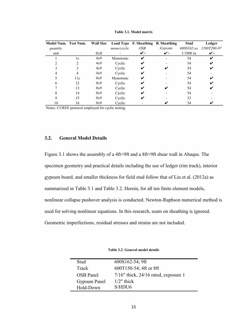
Figures 4.1 (a)-(j) show the nonlinear response of the developed computational models
compared with experimental results. Figure 4.1 (a) and (e) are for model 1 and model 5
which reproduce monotonic tests while the rest reproduces cyclic tests. A summary of
computational results including peak load and the corresponding lateral displacement is
provided in Table 4.1.
Overall, the shell finite element models predict the peak load with reasonable accuracy.
Except for model 9 which will be discussed later, the finite element models provide a
conservative prediction of the peak load for the specimens only sheathed by OSB and
provide an optimistic prediction for the specimens in which gypsum board is also
included. This suggests modeling gypsum board with its actual material properties

27
instead of the current assumption of semi-rigid diaphragm might create a more accurate
load distribution to the fasteners and provide a more encouraging and conservative
prediction of peak load for these models with gypsum board included.
As for model 9, while the specimen is not sheathed with gypsum board, the peak load
obtained from the finite element model is optimistic (13%). Compared with model 8, the
only difference in test configuration is a smaller thickness of 33mils is used for field
studs instead of a typical thickness of 54mils as used in all other tests. As shown in Table
4.1, the peak load obtained from computational modeling slightly decreases from 992plf
to 974plf when the thickness of field studs is reduced. However, this decrease is still too
small compared to the sudden drop in measured stiffness (peak load dropped from
1023plf down to 861plf) and results in an optimistic prediction of peak load. It is possible
that the impact of the field studs on the shear wall's overall response is not enough
accurately captured since the vertical OSB seam on the middle field stud is not included
in the model. It is also possible that the source of this discrepancy comes from the test
results when only one specimen is tested for each shear wall configuration. As described
by Liu et al. (2012a), this particular test with small thickness of field studs is an exception
whose capacity does not exceed or is within expected scatter (5%) of the shear strength
specified by design code. One can suggest conducting more tests with this configuration
in order to have a more thorough understanding of the impact of field stud size on a shear
wall's lateral capacity.
In general, the developed finite element models can accurately capture the initial stiffness
but become overly stiff afterwards. As a result, the lateral deflections at peak load
obtained from the developed models are somewhat smaller than the experimental values.

28
The likely source of this error is the hold-downs. In the shell finite element models, hold-
downs are modeled as springs located at the bottom areas on chord studs' web. This does
not take into account moment of the couple consisting of axial force in chord studs and
reaction force on the hold-down rod from the foundation because in the tests, the anchor
rod connecting hold-down to the foundation is slightly offset from the line along chord
studs' web. In addition, in some models, the analysis halts after the specimen reaches its
peak load due to convergence difficulty.
Table 4.1. Summary of computational results
Peak Load Lateral Deflection* Peak Load Lateral Deflection*
quantity P Δ P Δ
unit plf in. plf in.
1 1c 0.82 1003 1.97 1225 2.96
2 2 0.91 998 1.77 1102 2.82
3 3 1.14 1263 1.97 1111 2.67
4 4 0.97 974 1.77 1004 2.40
5 11c 0.98 1066 1.17 1089 2.42
6 12 0.91 1051 1.17 1156 1.96
7 13 1.09 1337 1.17 1232 1.91
8 14 0.97 992 1.09 1023 1.94
9 15 1.13 974 1.17 861 1.64
10 16 1.34 310 1.41 231 1.47
* Lateral deflection at peak load
Model Test Pcomp/PtestComputational Result Experimental Result
29
(a) (b)
(c) (d)
(e) (f)

30
(g) (h)
(i) (j)
Figure 4.1. Nonlinear response of computational models compared with experimental results: (a)-(j) for model 1-
model 10
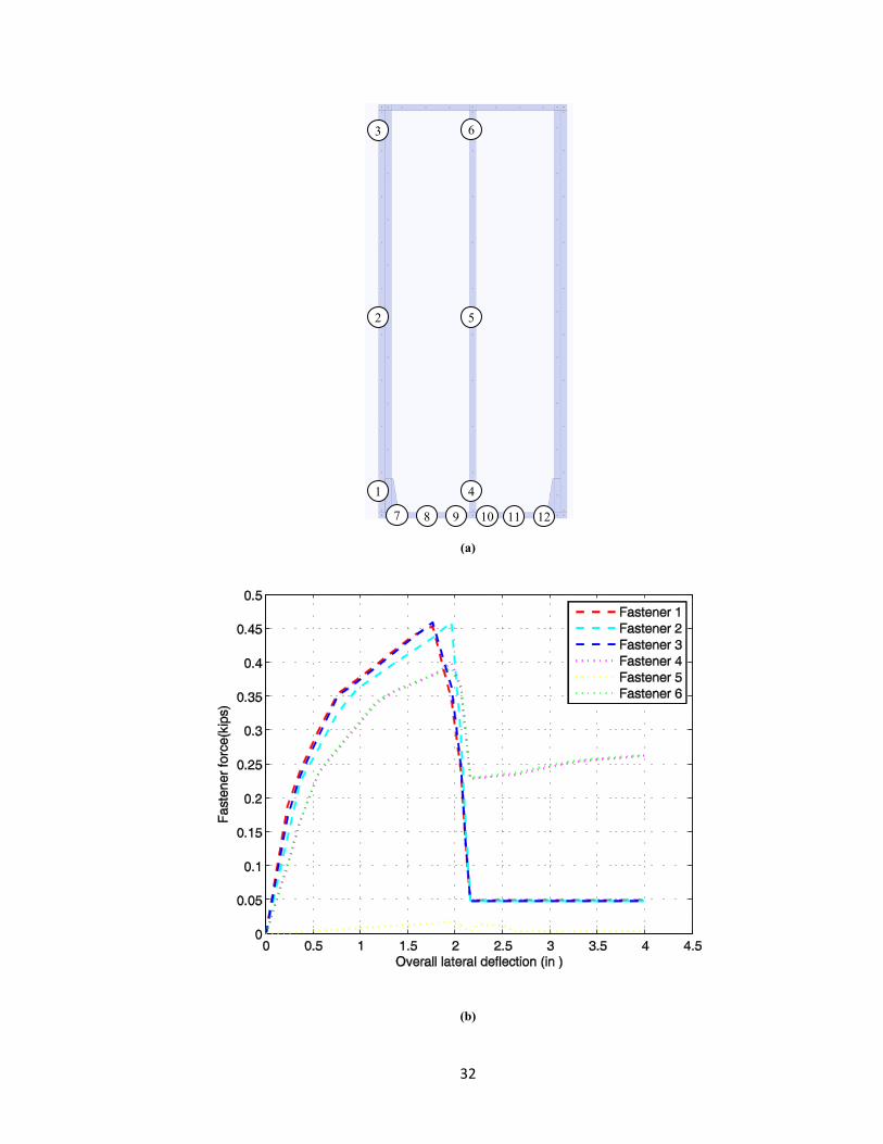
4.2. Sheathing-to-Frame Connection Failure
The developed finite element models allow the assessment of the manner in which shear
force in the shear wall is distributed to the fasteners. In particular, Figure 4.2 shows the
deformed shape of model 4 at the end of analysis with a focus on the deformation of the
sheathing-to-frame fasteners. Deformed shapes for all other models are provided in
Appendix A. Figures 4.3 (b)-(c) show the fastener force-overall lateral displacement

31
curve for some typical fasteners on left chord studs, field stud, and bottom track. The
location of these particular fasteners is provided in Figure 4.3 (a). Nonlinear response of
fasteners on top track and chord studs on the right side is not shown in the figures due to
the symmetry.
Force in fasteners on chord studs and tracks at the corner reaches its peak when the
overall shear wall specimen reaches its peak load at the lateral displacement of
approximately 1.75in. Fasteners at the middle of chord studs pass their maximum force a
little later at the overall lateral displacement of approximately 2in. The closer the fastener
on track is to the field stud, the less force is distributed to it. Fasteners at the middle of
tracks have not reached their maximum force and did not fail even at the end of analysis.
In the similar manner, failure at fasteners on field stud was not observed. Especially, very
little force is distributed to the fasteners at the middle of field stud. One interesting
observation from the deformed shape of model 4 is all the fasteners tend to deform in the
vertical direction.
Figure 4.2. Deformed shape of model 4 at the end of analysis (Scale factor: 2)
32
(a)
(b)
1
2
3
4
6
5
7 8 9 10 11 12

33
(c)
Figure 4.3. (a) Fastener location, (b) force in fasteners on stud, (c) force in fasteners on track
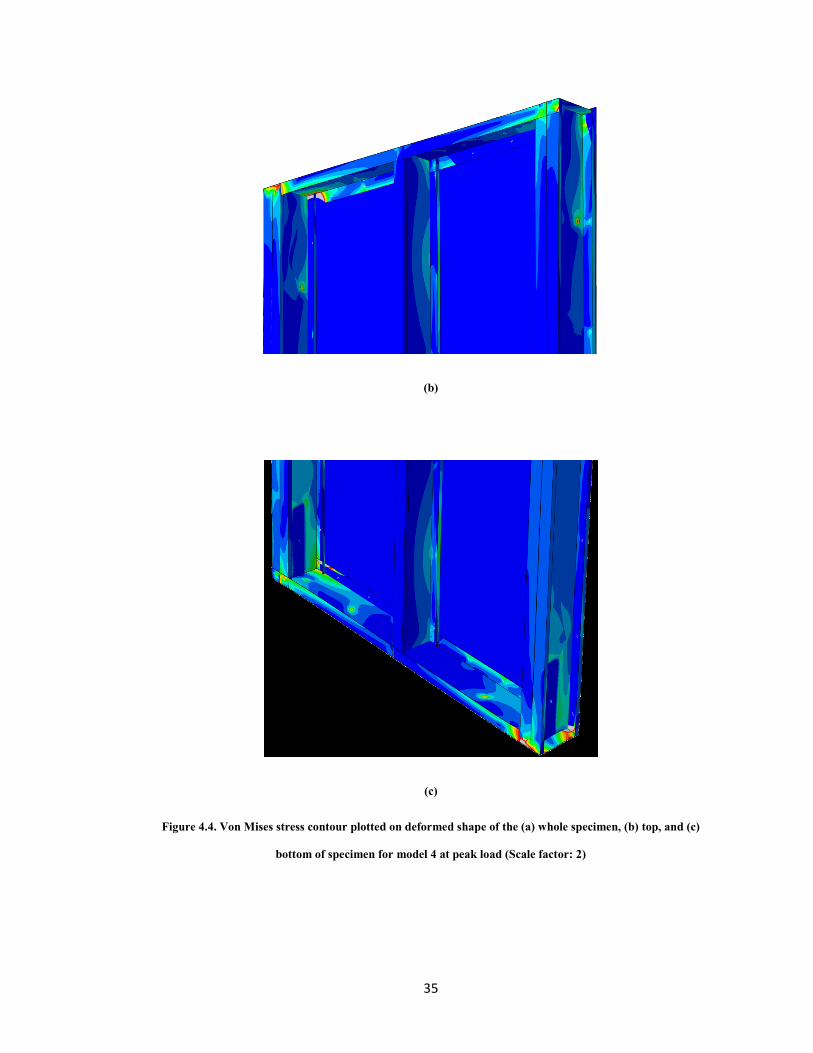
4.3. Deformation of Cold-Formed Steel Frame Members
One advantage of the developed high fidelity shell finite element models over other
nonlinear models is the ability to capture all the buckling modes of the cold-formed steel
frame members and visually represent the deformed shape and stress distribution in the
shear wall. In particular, Figure 4.4 (a)-(c) provides the von Mises stress contour plotted
on deformed shape of the specimen for model 4 at peak load. Rainbow color spectrum
from red (for the maximum value) to blue (for the minimum value) is used to represent
contour values. Grey color is used to represent the area whose stress being higher than the
maximum value. Von Mises stress is commonly used in determining whether an isotropic

34
metal yields when subjected to a complex loading condition. In this research, although
cold-formed steel members are modeled as elastic, the plotted contours can suggest
where to expect yielding to happen in the shear wall by setting the maximum limit for the
contour as material's yield stress. In particular, the maximum limit for the contours
provided in Figure 4.4 was set to be 50 ksi which is the actual yield stress of the cold-
formed steel used for the test. The plots show a large stress concentration on the flanges
of tracks near the stud-to-track connection (represented by grey color) and indicate that
these areas should be expected to yield according to von Mises Yield Criterion. One
might suggest employing strain gauges to further explore the deformation of steel
members at these locations in future testing.
(a)
35
(b)
(c)
Figure 4.4. Von Mises stress contour plotted on deformed shape of the (a) whole specimen, (b) top, and (c)
bottom of specimen for model 4 at peak load (Scale factor: 2)

36
4.4. Summary
Chapter 4 provided the computational results for ten high fidelity shell finite element
models whose protocol is detailed in Chapter 3. Overall, the developed models can
predict the peak load with reasonable accuracy but is overly stiff. The failure mechanism
of sheathing-to-frame connections and deformation of cold-formed steel frame members
were also presented.

37
Chapter 5 - Experimental Setup
This chapter details the experimental setup for future full-scale shear wall tests.
Specifically, modified testing rig, sensor plan, loading protocol, assembly of typical test
specimen, and preparation for future material testing will be presented.
5.1. Testing Rig
The Johns Hopkins University multi-degree of freedom testing rig, which is called Big
Blue Baby, will be used for conducting future full-scale shear wall tests. As depicted in
Figure 5.1, this rig consists of one horizontal hydraulic actuator, two lateral hydraulic
actuators, and four vertical hydraulic actuators. This allows the specimen to be loaded
with any combinations of axial load, shear, and bending.
Figure 5.1. Modified Big Blue Baby with 8 ft × 8ft shear wall specimen

38
Design of top and bottom steel tubes
In order to connect the shear wall specimen to the rig, one steel tube at the top and one
steel tube at the bottom were designed and fabricated. As depicted in Figures 5.2 (a)-(b),
holes were drilled on the top and bottom surface of each tube so that one can connect
these tubes to the Big Blue Baby and bolt the specimen's tracks to these tubes prior to the
test. Both tubes have cut-outs along the length to provide access to the bolts just
mentioned. The design of two steel tubes was conducted in a conservative manner based
on the limit states of moment yielding, shear yielding, and deflection taking into
consideration of the hold-down force and gravity load applied to the specimen.
Rectangular hollow structural section (HSS) 10×4×1/2 was used for both two tubes.
Detailed drawings of these tubes are provided in Appendix B.

39
(a) (b)
Figure 5.2. Modification to existing testing rig (a) top tube, (b) bottom tube
Design of steel bars for hold-downs and steel plates
During the test, a large force is expected be transferred from the specimen to the steel
tube passing hold-down anchor rod. The concentration of this hold-down force on a
small area on steel tube at the location of hold-down anchor rod can cause significant
deformation. For this reason, steel bars were designed to distribute this force to a larger
area on tubes as described in Figure 5.3 (a)-(b).

40
In order to avoid the contact between sheathing and the testing rig during the test, steel
plates are designed and fabricated. These steel plates, as shown in Figure 5.3 (c) will be
placed between specimen and the steel tubes.
Detailed drawings of these steel bars and plates are provided in Appendix B.
(a)
(b)

41
(c)
Figure 5.3. (a)-(b) Steel bars for hold-downs, (c) steel plates
5.2. Instrumentation Plan
Eight sensors were employed to measure the response of the specimen under loading.
Sensor layout and numbering scheme are provided in Figure 5.4. Position
transducers 1 and 2 measure lateral displacement at the top and bottom of the shear wall.
Relative displacement between chord stud ends and tracks in vertical direction are
captured by position transducers 3,4,5, and 6. Position transducers 7 and 8 record vertical
motion of the loading beam. As depicted in Figure 5.5, seven position transducers are
installed using magnetic mounting base. Only position transducer 2 is mounted on a
plastic plate which is clamped to the bottom tube. One advantage of this sensor plan is
that some sensors do not have to be removed and reinstalled between tests. Also, due to
the use of magnetic mounting base, the installation is quick and simple.

42
Figure 5.4. Instrumentation plan
Figure 5.5. Installation of position transducer
1
2
3
4 6
5
7
8

43
5.3. Load Protocol
All of the shear walls are subjected to a combination of lateral and vertical loads using
displacement control. Lateral loading can either be monotonic or cyclic. Monotonic test is
first conducted in order to determine the ultimate displacement which will be used as
target maximum deformation for cyclic test. Cyclic loading is in accordance with the
FEMA 461 quasi-static cyclic testing protocol. This protocol is chosen because it can be
used to obtain not only fragility data but also data on the hysteretic characteristics of the
structural components of which damage is best predicted by imposed deformations.
FEMA 461 protocol consists of steps with increasing amplitude and two identical cycles
need to be completed for each amplitude. Amplitude of one step is 1.4 times larger than
that of the previous step. Lateral displacement at the top of the shear wall is used as
deformation control parameter. The FEMA 461 protocol is defined in order that a
deformation associated with the most severe damage state (ultimate displacement
measured from monotonic test) is reached at the 10th step. Further information can be
found at "Interim Testing Protocols for Determining the Seismic Performance
Characteristics of Structural and Nonstructural Components" (2007).
5.4. Typical Test Specimen
Figures 5.6 (a),(b) depict the dimension and fastener schedule for 4ft × 8ft and 8ft × 8ft
shear wall specimen. Figure 5.7 shows a typical 4ft × 8ft shear wall specimen assembled
by the author and colleagues at Thin-walled Structures Laboratory, Johns Hopkins
University.

44
(a) (b)
Figure 5.6. Drawing of (a) 4ft × 8ft, (b) 8ft × 8ft shear wall specimens
Figure 5.7. Assembly of 4ft × 8ft shear wall specimen at Thin-walled Structures Laboratory, Johns Hopkins
University

45
5.5. Material Properties
In order to prepare for future material tensile testing, specimens were cut from the webs
of cold-formed steel channel sections (362S162-54 [50ksi] and 362T150-54 [50ksi]) and
then precision machined into tensile coupons as depicted in Figure 5.8 (a). Specifically,
three coupons were obtained from one cold-formed steel member. These uncoated
coupons will be tested using the MTS machine shown in Figure 5.8 (b).
(a)
(b)
Figure 5.8. Preparation for material tensile testing (a) tensile specimens, (b) MTS machine

46
Chapter 6 - Future Work
The high fidelity computational models described herein were demonstrated to be able to
simulate wood-sheathed cold-formed steel shear walls with reasonable accuracy.
However, this developed modeling protocol can be further improved by (i) modeling
gypsum board with its actual material properties, (ii) incorporating unloading/reloading
(pinching) behavior so that the full non-linear cyclic response can be reproduced, (iii)
explicitly modeling the hold-downs to take into account the hold-down force eccentricity,
and (iv) including geometric imperfections, residual stresses and strains.
As the continuation of the first phase, phase two of the overall project needs to be
conducted. The scope of phase 2 is as follows.
(a) Parametric study of wood-sheathed cold-formed steel framed shear walls with non-
conventional detailing based on developed modeling protocol
(b) Full-scale testing on wood-sheathed cold-formed steel framed shear walls with non-
conventional detailing

47
Chapter 7 - Conclusions
The objective of the overall project is to explore limit states other than those associated
with the fastener, such as chord buckling, in the wood-sheathed cold-formed steel framed
shear wall so that reliability of this complex subsystem can formally be evaluated based
on potential limit states. This thesis presented phase 1 of this project focusing on the
development of high fidelity computational modeling of wood-sheathed cold-formed
steel framed shear walls and preparation for future full-scale shear wall testing.
A series of ten high fidelity shell finite element models were initiated in Abaqus to
simulate ten CFS-NEES shear wall specimens tested by Liu et al. (2012a,b). The
developed modeling protocol was demonstrated to be able to capture lateral capacity with
reasonable accuracy. The predicted strength was conservative for the shear walls only
sheathed by OSB and slightly optimistic when gypsum board is also included. In general,
initial stiffness was accurately captured but the models became overly stiff afterwards. As
a result, lateral deflections at peak load obtained from the developed models were
somewhat smaller than the experimental values. In addition, failure mechanism of
sheathing-to-frame connections and deformation of cold-formed steel frame members
were presented. A large stress concentration was observed at the flanges of tracks near
the stud-to-track connection. While improvements are recommended, the agreement in
response with the tests was considered encouraging given that the fastener data were
obtained from tests conducted completely independently from Liu et al. (2012a,b)'s tests.

48
Experimental setup for future full-scale shear wall testing was also presented.
Specifically, modified testing rig, sensor plan, loading protocol, assembly of typical test
specimen, and preparation for future material testing were described.
As the continuation of the research presented herein, phase two of the overall project
including parametric study and full-scale testing on shear walls with non-conventional
detailing are underway.

49
Appendix A - Deformed Shape Of Computational Models

50
Figure A.1. Deformed shape of model 1c at the end of analysis (Front view, scale factor: 2)
Figure A.2. Deformed shape of model 2 at the end of analysis (Front view, scale factor: 2)

51
Figure A.3. Deformed shape of model 3 at the end of analysis (Front view, scale factor: 2)
Figure A.4. Deformed shape of model 4 at the end of analysis (Front view, scale factor: 2)

52
Figure A.5. Deformed shape of model 11c at the end of analysis (Front view, scale factor: 2)
Figure A.6. Deformed shape of model 12 at the end of analysis (Front view, scale factor: 2)

53
Figure A.7. Deformed shape of model 13 at the end of analysis (Front view, scale factor: 2)
Figure A.8. Deformed shape of model 14 at the end of analysis (Front view, scale factor: 2)

54
Figure A.9. Deformed shape of model 15 at the end of analysis (Front view, scale factor: 2)
Figure A.10. Deformed shape of model 16 at the end of analysis (Back view, scale factor: 2)

55
Appendix B - AutoCAD Drawings

56
Figure B.1. Drawing of bottom tube

57
Figure B.2. Drawing of top tube
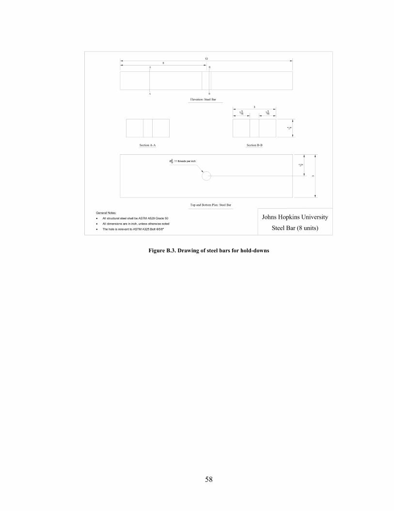
58
Figure B.3. Drawing of steel bars for hold-downs

59
Figure B.4. Drawing of steel plate 1

60
Figure B.5. Drawing of steel plate 2

61
Figure B.6. Drawing of steel plate 3

62
Figure B.7. Drawing of steel plate 4

63
References
Liu, P., Peterman, K.D., Schafer, B.W. (2012a). “Test Report on Cold-Formed Steel
Shear Walls”, Research Report, CFS-NEES, RR03.
Liu, P., Peterman, K.D., Yu, C., Schafer, B.W. (2012b). “Characterization of cold-formed
steel shear wall behavior under cyclic loading for the CFS-NEES building.” Proc. of the
21st Int’l. Spec. Conf. on Cold-Formed Steel Structures, 24-25 October 2012, St. Louis,
MO, 703-722.
Peterman, K.D., Schafer, B.W. (2013).“Hysteretic shear response of fasteners connecting
sheathing to cold-formed steel studs.” Research report, CFS-NEES, RR04.
Buonopane,S.G., Tun, T. H., Schafer, B.W.(2014).“Fastener-based computational models
for prediction of seismic behavior of CFS shear walls.” 10th US National Conference on
Earthquake, Anchorage, Alaska.
Leng, J., Schafer, B.W., Buonopane, S.G. (2013). “Modeling the seismic response of
cold-formed steel framed buildings: model development for the CFS-NEES building.”
Proceedings of the Annual Stability Conference - Structural Stability Research Council,
St. Louis, Missouri, April 16-20, 2013, 17pp.
Madsen,R.L., Nakata, N., Schafer,B.W.(2011).“CFS-NEES Building Structural Design
Narrative.” Research report, CFS-NEES, RR01.
Peterman, K.D., Madsen, R.L., Schafer, B.W.(2014). “Experimental seismic behavior of
the CFS-NEES building: system-level performance of a full-scale two-story light steel

64
framed building.” Twenty-second International Specialty Conference on Cold-Formed
Steel Structures, St. Louis, Missouri
Schafer, B.W., Li, Z., Moen, C.D. (2010).“Computational modeling of cold-formed
steel.” Thin-Walled Structures,48(2010): 752–762.
A.E. Branston, C.Y. Chen, F.A. Boudreault, and C.A. Rogers (2006).“ Testing of light-
gauge steel-frame – wood structural panel shear walls” Canadian Journal of Civil
Engineering, 33: 561–572 (2006)
Boudreault, F.A. 2005. “Seismic analysis of steel frame / wood panel shear walls”
M.Eng. thesis, Department of Civil Engineering and Applied Mechanics, McGill
University, Montréal, Que.
Branston, A.E., Boudreault, F.A., Chen, C.Y., and Rogers, C.A. 2004. “Light gauge steel
frame / wood panel shear wall test data”. Research Report, Department of Civil
Engineering and Applied Mechanics, McGill University, Montréal, Que.
Chen, C.Y. 2004. “Testing and performance of steel frame / wood panel shear walls”.
M.Eng. thesis, Department of Civil Engineering and Applied Mechanics, McGill
University, Montréal, Que.
Chen, C.Y., Boudreault, F.A., Branston, A.E., and Rogers, C.A. 2005. “Behaviour of
light gauge steel-frame – wood structural panel shear walls”. Canadian Journal of Civil
Engineering, 33: 573–587.
ABAQUS. ABAQUS/Standard User’s Manual, Version 6.9 EF1. Pawtucket, RI; 2009.

65
AISI S213-07: “North American Standard for Cold-Formed Steel Farming - Lateral
Design”, (2007 edition). American Iron and Steel Institute, Washington, D.C.
ANSI/AISI-S213-07. 2007.
ASTM E2126 (2011). “Standard Test Methods for Cyclic (Reversed) Load Test for Shear
Resistance of Vertical Elements of the Lateral Force Resisting Systems for Buildings,”
ASTM International, West Conshohocken, PA, 2006, DOI: 10.1520/E2126-11,
www.astm.org.
ASTM E564 (2006). “Standard Practice for Static Load Test for Shear Resistance of
Framed Walls for Buildings,” ASTM International, West Conshohocken, PA, 2006, DOI:
10.1520/E0564-06, www.astm.org.
ASTM A370 (2006) “Standard Test Methods and Definitions for Mechanical Testing of
Steel Products,” American Association State Highway and Transportation Officials
Standard, AASHTO No.: T 244
FEMA, FEMA 461 - Interim protocols for determining seismic performance
characteristics of structural and nonstructural components through laboratory testing,
Federal Emergency Management Agency (FEMA), Document No. FEMA 461. 2007.

66
Curriculum Vitae
Hung Huy Ngo was born in Nghe An, Vietnam on November 9th, 1986. He received a
Bachelor of Civil Engineering from the University of Kyoto, Japan in March 2011. After
graduation, he joined the International Division of Japan Transportation Consultants, Inc.,
Japan as a civil engineer. His main role was to collaborate with leadership to compile
civil engineering project proposals and provide technical support to the company's
international projects. He also directly participated in several international projects in
Asian countries including Vietnam and Indonesia.
In September 2012, Hung started his graduate studies at the Johns Hopkins University
and is a candidate for the degree of Master of Science in Engineering from the
department of Civil Engineering in August 2014.
During his academic career, Hung has been awarded many fellowships due to excellent
performance such as Japanese Government (MEXT) Scholarship (2006 - 2011) and
Vietnam Education Foundation Fellowship (2012-2014).