Embed Size (px)
Citation preview

Numerical and Experimental Investigation of
Membrane Distillation Flux and Energy Efficiency
by
Jaichander Swaminathan
B. Tech., Indian Institute of Technology Madras (2012)
Submitted to the Department of Mechanical Engineeringin partial fulfillment of the requirements for the degree of
Master of Science in Mechanical Engineering
at the
MASSACHUSETTS INSTITUTE OF TECHNOLOGY
June 2014
c© Massachusetts Institute of Technology 2014. All rights reserved.
Author . . . . . . . . . . . . . . . . . . . . . . . . . . . . . . . . . . . . . . . . . . . . . . . . . . . . . . . . . . . . . .Department of Mechanical Engineering
May 18, 2014
Certified by. . . . . . . . . . . . . . . . . . . . . . . . . . . . . . . . . . . . . . . . . . . . . . . . . . . . . . . . . .John H. Lienhard V
Collins Professor of Mechanical EngineeringThesis Supervisor
Accepted by . . . . . . . . . . . . . . . . . . . . . . . . . . . . . . . . . . . . . . . . . . . . . . . . . . . . . . . . .David E. Hardt
Chairman, Committee on Graduate Theses

2
Numerical and Experimental Investigation of Membrane
Distillation Flux and Energy Efficiency
by
Jaichander Swaminathan
Submitted to the Department of Mechanical Engineeringon May 18, 2014, in partial fulfillment of the
requirements for the degree ofMaster of Science in Mechanical Engineering
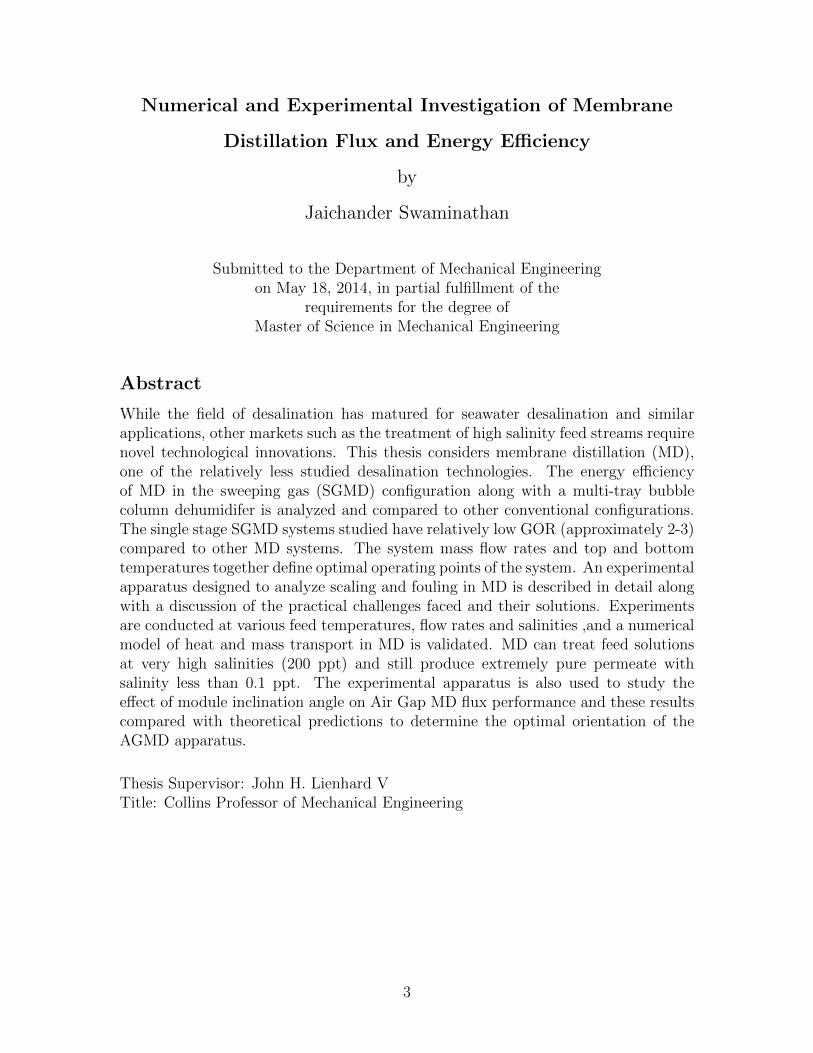
Abstract
While the field of desalination has matured for seawater desalination and similarapplications, other markets such as the treatment of high salinity feed streams requirenovel technological innovations. This thesis considers membrane distillation (MD),one of the relatively less studied desalination technologies. The energy efficiencyof MD in the sweeping gas (SGMD) configuration along with a multi-tray bubblecolumn dehumidifer is analyzed and compared to other conventional configurations.The single stage SGMD systems studied have relatively low GOR (approximately 2-3)compared to other MD systems. The system mass flow rates and top and bottomtemperatures together define optimal operating points of the system. An experimentalapparatus designed to analyze scaling and fouling in MD is described in detail alongwith a discussion of the practical challenges faced and their solutions. Experimentsare conducted at various feed temperatures, flow rates and salinities ,and a numericalmodel of heat and mass transport in MD is validated. MD can treat feed solutionsat very high salinities (200 ppt) and still produce extremely pure permeate withsalinity less than 0.1 ppt. The experimental apparatus is also used to study theeffect of module inclination angle on Air Gap MD flux performance and these resultscompared with theoretical predictions to determine the optimal orientation of theAGMD apparatus.
Thesis Supervisor: John H. Lienhard VTitle: Collins Professor of Mechanical Engineering
3

4

Acknowledgments
I am grateful to my advisor, Prof. John Lienhard for his guidance throughout the
course of this project.
I would like to thank Edward Summers for sharing his MD numerical models and
his experimental expertise. Thanks David, for being a great co-researcher. Thanks
to all my lab-mates for their continuous encouragement and for providing useful
feedback.
I would like to thank our collaborators at Masdar University, Prof. Hassan A.
Arafat and Dr. Elena Guillen-Burrieza for sharing their insights and helping out
along the way.
I would like to acknowledge the contributions of MIT undergraduate students
Sarah Ritter, Laith Maswadeh, Aileen Guttman, Joanna K. So and Sterling Watson
in the design and building of several components of the experimental setup described
in this thesis.
This work was funded by the Cooperative Agreement between the Masdar In-
stitute of Science and Technology (Masdar Institute), Abu Dhabi, UAE and the
Massachusetts Institute of Technology (MIT), Cambridge, MA, USA - Reference
02/MI/MI/CP/11/07633/GEN/G/00.
5

6

Contents
1 Introduction 19
1.1 Need for Alternate Desalination Technologies . . . . . . . . . . . . . . 19
1.2 Membrane Distillation for Desalination . . . . . . . . . . . . . . . . . 21
1.3 Fouling in Membrane Distillation . . . . . . . . . . . . . . . . . . . . 22
2 Energy Efficiency of Sweeping Gas Membrane Distillation Systems 25
2.1 Introduction . . . . . . . . . . . . . . . . . . . . . . . . . . . . . . . . 25
2.1.1 SGMD Process . . . . . . . . . . . . . . . . . . . . . . . . . . 27
2.1.2 Bubble Column Dehumidifier (BCDH) Process . . . . . . . . . 27
2.2 Modeling . . . . . . . . . . . . . . . . . . . . . . . . . . . . . . . . . . 29
2.2.1 SGMD Module . . . . . . . . . . . . . . . . . . . . . . . . . . 29
2.2.2 Multi-tray Bubble Column Dehumidifier . . . . . . . . . . . . 33
2.3 Validation . . . . . . . . . . . . . . . . . . . . . . . . . . . . . . . . . 34
2.4 SGMD and MBCD System Analysis . . . . . . . . . . . . . . . . . . . 38
2.4.1 Entropy Generation and GOR . . . . . . . . . . . . . . . . . . 38
2.4.2 SGMD Module . . . . . . . . . . . . . . . . . . . . . . . . . . 39
2.4.3 Multi-tray Bubble Column Dehumidifier . . . . . . . . . . . . 43
2.5 Cycle Analysis . . . . . . . . . . . . . . . . . . . . . . . . . . . . . . . 43
2.5.1 Mass Flow Rates . . . . . . . . . . . . . . . . . . . . . . . . . 46
2.5.2 Temperatures . . . . . . . . . . . . . . . . . . . . . . . . . . . 47
2.5.3 Geometry . . . . . . . . . . . . . . . . . . . . . . . . . . . . . 49
2.5.4 Dehumidifer Effectiveness . . . . . . . . . . . . . . . . . . . . 54
2.5.5 Membrane Properties . . . . . . . . . . . . . . . . . . . . . . . 54
7

2.5.6 Further Improvements . . . . . . . . . . . . . . . . . . . . . . 55
2.6 Conclusions . . . . . . . . . . . . . . . . . . . . . . . . . . . . . . . . 55
3 Experimental Design of Air Gap Membrane Distillation System for
Fouling Tests 57
3.1 Introduction . . . . . . . . . . . . . . . . . . . . . . . . . . . . . . . . 57
3.2 Design Criteria . . . . . . . . . . . . . . . . . . . . . . . . . . . . . . 58
3.2.1 Module Type . . . . . . . . . . . . . . . . . . . . . . . . . . . 59
3.2.2 MD Configuration . . . . . . . . . . . . . . . . . . . . . . . . 60
3.2.3 Feed Reynolds Number . . . . . . . . . . . . . . . . . . . . . . 61
3.2.4 Membrane Area . . . . . . . . . . . . . . . . . . . . . . . . . . 61
3.2.5 Air Gap . . . . . . . . . . . . . . . . . . . . . . . . . . . . . . 62
3.2.6 Feed, Cold Water . . . . . . . . . . . . . . . . . . . . . . . . . 63
3.2.7 Module assembly . . . . . . . . . . . . . . . . . . . . . . . . . 64
3.2.8 Feed Channel . . . . . . . . . . . . . . . . . . . . . . . . . . . 67
3.2.9 Membrane . . . . . . . . . . . . . . . . . . . . . . . . . . . . . 68
3.2.10 Piping and Pumps . . . . . . . . . . . . . . . . . . . . . . . . 69
3.3 Instrumentation . . . . . . . . . . . . . . . . . . . . . . . . . . . . . . 69
3.3.1 Temperature . . . . . . . . . . . . . . . . . . . . . . . . . . . . 69
3.3.2 Flow Rates . . . . . . . . . . . . . . . . . . . . . . . . . . . . 70
3.3.3 Mass/Flux . . . . . . . . . . . . . . . . . . . . . . . . . . . . . 70
3.3.4 Conductivity . . . . . . . . . . . . . . . . . . . . . . . . . . . 71
3.4 Modeling . . . . . . . . . . . . . . . . . . . . . . . . . . . . . . . . . . 71
3.4.1 Concentration Polarization . . . . . . . . . . . . . . . . . . . . 71
3.5 Results and Discussion . . . . . . . . . . . . . . . . . . . . . . . . . . 73
3.5.1 Parametric Studies . . . . . . . . . . . . . . . . . . . . . . . . 73
3.5.2 Other Experimental Issues . . . . . . . . . . . . . . . . . . . . 77
3.6 Conclusions . . . . . . . . . . . . . . . . . . . . . . . . . . . . . . . . 82
4 Effect of Module Inclination Angle on Air Gap Membrane Distilla-
tion Flux 85
8
4.1 Introduction . . . . . . . . . . . . . . . . . . . . . . . . . . . . . . . . 86
4.2 Apparatus Design . . . . . . . . . . . . . . . . . . . . . . . . . . . . . 88
4.3 Numerical Modeling . . . . . . . . . . . . . . . . . . . . . . . . . . . 88
4.3.1 Modeling Methods and Feed Channel Modeling . . . . . . . . 88
4.3.2 Air Gap and Condensing Channel Modeling . . . . . . . . . . 90
4.3.3 Modeling Inputs . . . . . . . . . . . . . . . . . . . . . . . . . 91
4.3.4 Effect of Module Tilt Angle . . . . . . . . . . . . . . . . . . . 91
4.4 Methodology . . . . . . . . . . . . . . . . . . . . . . . . . . . . . . . 92
4.4.1 Experimental Methodology . . . . . . . . . . . . . . . . . . . . 92
4.4.2 Uncertainty Quantification . . . . . . . . . . . . . . . . . . . . 93
4.5 Experimental Results . . . . . . . . . . . . . . . . . . . . . . . . . . . 94
4.5.1 Effect of Angle on Permeate Flux . . . . . . . . . . . . . . . . 94
4.5.2 Thermal Bridging Hypothesis . . . . . . . . . . . . . . . . . . 98
4.6 Conclusions . . . . . . . . . . . . . . . . . . . . . . . . . . . . . . . . 100
9

10

List of Figures
1-1 Contributions of different technologies to total worldwide installed de-
salination capacity as of 2012 . . . . . . . . . . . . . . . . . . . . . . 20
1-2 Schematic diagram of various membrane distillation systems (from [1]) 22
2-1 Schematic diagram of SGMD process . . . . . . . . . . . . . . . . . . 27
2-2 Schematic diagram of BCDH process . . . . . . . . . . . . . . . . . . 28
2-3 SGMD computational cell with heat and mass fluxes and associated
boundary layers . . . . . . . . . . . . . . . . . . . . . . . . . . . . . . 30
2-4 Schematic diagram of MBCD system with four stages . . . . . . . . . 34
2-5 Temperature vs. position for a MBCD system showing the terminal
temperature difference (TTD) . . . . . . . . . . . . . . . . . . . . . . 35
2-6 Flux vs. temperature of feed inlet compared with experimental data . 36
2-7 Flux prediction . . . . . . . . . . . . . . . . . . . . . . . . . . . . . . 37
2-8 Specific entropy generation as a function of inlet air temperature. Hu-
midity = ωsat(25 ◦C) . . . . . . . . . . . . . . . . . . . . . . . . . . . 39
2-9 Air stream state . . . . . . . . . . . . . . . . . . . . . . . . . . . . . . 41
2-10 Temperature vs. position . . . . . . . . . . . . . . . . . . . . . . . . . 42
2-11 Vapor pressure vs. position . . . . . . . . . . . . . . . . . . . . . . . 44
2-12 Specific entropy generation in a MBCD. (Ta,in = 50 ◦C, mc= 0.189 kg/s,
Tc,in= 25 ◦C) . . . . . . . . . . . . . . . . . . . . . . . . . . . . . . . . 45
2-13 Complete SGMD-MBCD desalination system . . . . . . . . . . . . . . 47
2-14 GOR dependence on mass flow rates . . . . . . . . . . . . . . . . . . 48
2-15 GOR dependence on cycle top temperature . . . . . . . . . . . . . . . 50
11

2-16 GOR dependence on cycle bottom temperature . . . . . . . . . . . . 51
2-17 GOR dependence on length and width . . . . . . . . . . . . . . . . . 52
2-18 GOR dependence on channel depth . . . . . . . . . . . . . . . . . . . 53
2-19 Effect of number of BCDH stages . . . . . . . . . . . . . . . . . . . . 54
2-20 Effect of membrane permeability . . . . . . . . . . . . . . . . . . . . 55
2-21 GOR vs. feed mass flow rate. L = 60 m . . . . . . . . . . . . . . . . 56
3-1 A schematic diagram of the MD experimental setup . . . . . . . . . . 59
3-2 GOR comparison between single stage MD configurations [2] . . . . . 60
3-3 MD membrane during operation: regions of the membrane are pushed
into the gaps in the mesh spacer . . . . . . . . . . . . . . . . . . . . . 63
3-4 MD assembly showing individual components. Left to right: Metal
flange, feed plate, MD membrane, plastic spacer with mesh spacer,
condensing plate and cooling channel . . . . . . . . . . . . . . . . . . 64
3-5 Design of quick release clamps for easy access to membrane between
tests . . . . . . . . . . . . . . . . . . . . . . . . . . . . . . . . . . . . 65
3-6 A thinner spacer stacked over the woven mesh in the air-gap . . . . . 66
3-7 Feed channel design . . . . . . . . . . . . . . . . . . . . . . . . . . . . 67
3-8 Design of inlet manifold with high pressure reservoir and outflow noz-
zles for uniform outflow. All dimensions are in mm . . . . . . . . . . 68
3-9 Water production rate as a function of feed inlet salinity. Tf = 69.5 ◦C, Vf =
0.2558 L/s . . . . . . . . . . . . . . . . . . . . . . . . . . . . . . . . . 74
3-10 Water production rate as a function of feed inlet salinity. Tf = 70 ◦C, Vf =
0.252 kg/s . . . . . . . . . . . . . . . . . . . . . . . . . . . . . . . . . 75
3-11 Effect of temperature on permeate production rate. S = 191 ppt, Vf =
0.252 L/s . . . . . . . . . . . . . . . . . . . . . . . . . . . . . . . . . . 76
3-12 Effect of temperature on permeate production rate. S = 198 ppt, Vf =
0.2678 L/s . . . . . . . . . . . . . . . . . . . . . . . . . . . . . . . . . 77
3-13 Effect of feed flow rate on flux. Model data for 0 ppt included for
reference. S = 44 ppt,Tf = 70 ◦C . . . . . . . . . . . . . . . . . . . . 78
12

3-14 Effect of flow rate on flux. Feed flow rate varied from 0.032 L/s to
0.315 L/s. S = 70 ppt,Tf = 69.5 ◦C . . . . . . . . . . . . . . . . . . . 79
3-15 Flux as a function of temperature and flow rate. S=100 ppt . . . . . 80
3-16 Flux as a function of temperature and flow rate. S=2 ppt . . . . . . . 81
3-17 Rust seen on heater element in CaSO4 supersaturation experiments . 82
3-18 Membrane used for experiment (Fig. 3-10) showing discoloration . . . 83
3-19 Heater separated from feed tank using a plastic bag . . . . . . . . . . 84
4-1 AGMD at varied angles . . . . . . . . . . . . . . . . . . . . . . . . . . 87
4-2 Computational cell of the AGMD model from [2]. . . . . . . . . . . . 89
4-3 Effect of module tilt angle on flux predicted by model . . . . . . . . . 92
4-4 Effect of module tilt angle on permeate production: Tf,in = 50 ◦C, Tc,in
= 12.5 ◦C . . . . . . . . . . . . . . . . . . . . . . . . . . . . . . . . . 95
4-5 Effect of module tilt angle on permeate production: Tf,in = 60 ◦C, Tc,in
= 40 ◦C. . . . . . . . . . . . . . . . . . . . . . . . . . . . . . . . . . . 96
4-6 Effect of module tilt angle on permeate production: Smaller air gap.
Tf,in = 50 ◦C, Tc,in = 20 ◦C. . . . . . . . . . . . . . . . . . . . . . . . . 97
4-7 Effect of module tilt angle on permeate production: Smaller air gap.
Tf,in = 60 ◦C, Tc,in = 40 ◦C. . . . . . . . . . . . . . . . . . . . . . . . . 98
4-8 Effect of module tilt angle on permeate production: Comparison with
modified experiment where hydrostatic forced flooding is avoided. Tf,in
= 50 ◦C, Tc,in = 20 ◦C . . . . . . . . . . . . . . . . . . . . . . . . . . . 99
13

14

List of Tables
2.1 Baseline values for validation test cases . . . . . . . . . . . . . . . . . 38
2.2 Baseline values of SGMD desalination system . . . . . . . . . . . . . 49
3.1 Uncertainty in flux as a function of uncertainty in measured parameters
(using EES). An uncertainty of 0.05 mm in dgap contributes to more
than 75 % of the uncertainty in flux . . . . . . . . . . . . . . . . . . . 62
15

Nomenclature
Roman symbols Units
B membrane distillation coefficient kg/m2 s Pa
cp specific heat at constant pressure J/kgK
d channel depth m
dA area element m2
dz elemental length m
h specific enthalpy J/kg
hfg enthalpy of vaporization J/kg
J mass flux kg/m2 s
kmass mass transfer coefficient m/s
L module effective length m
m mass flow rate kg/s
mr air water mass flow rate ratio -
MW molecular weight kg/kmol
ncells number of computational cells -
P pressure Pa
p partial pressure Pa
q heat flux W/m2
Q rate of heat addition W
s specific entropy J/kg K
S, sal salinity g/kg
Sgen entropy generation rate W/K
sgen specific entropy generation J/kg K
T temperature oC
v velocity m/s
w module width m
x mole fraction -
z distance along module length m
16
Greek symbols
α heat transfer coefficient W/m2 K
δ thickness of membrane m
δ film thickness in AGMD m
ε porosity %
γ activity coefficient
ω humidity ratio kg/kg
ρ density kg/m3
Subscripts
(·)a air
(·)b bulk/free stream
(·)c coolant
(·)da dry air
(·)eff effective
(·)f feed
(·)gap air gap
(·)in inlet
(·)m membrane
(·)out outlet
(·)p permeate
(·)sg sweeping gas
(·)v vapor
(·)vap vapor pressure
(·)wb wet bulb
(·)w water
Acronyms
AGMD Air Gap Membrane Distillation
BCDH Bubble Column Dehumidifier
DCMD Direct Contact Membrane Distillation
DBT Dry Bulb Temperature ◦C
17
EES Engineering Equation Solver
GOR Gained Output Ratio -
MD Membrane Distillation
MSBCDH Multistage Bubble Column Dehumidifier
SGMD Sweeping Gas Membrane Distillation
VMD Vacuum Membrane Distillation
MD Membrane Distillation
MED Multiple Effect Distillation
MSF Multiple Stage Flash
ppt Parts per thousand g/kg
ppm Parts per million mg/kg
TTD Terminal Temperature Difference ◦C
18

Chapter 1
Introduction
Desalination technologies are being used today as a source of fresh water in water
stressed regions of the world that have access to sea or brackish water. With rapidly
growing populations and increasing energy use and standards of living, more regions
of the world are getting water stressed [3]. Increased water reuse and improvements
in efficiency of water purification and desalination technologies can help tackle these
problems.
Significant improvements have been made in desalination technologies since their
first appearance. Membrane research for reverse osmosis (RO) has resulted in a sharp
reduction in membrane manufacturing costs and an increase in membrane permeabil-
ity, leading to RO dominating the seawater desalination market at present. More the
60 % of the desalination installations in the world as of 2012 have are RO plants and
this fraction is steadily increasing [4] (Fig. 1-1). A study by Mistry et al. [5] showed
that in terms of second law efficiency, RO is way ahead of most other technologies
with lower relative irreversibilities.
1.1 Need for Alternate Desalination Technologies
In addition to producing pure permeate water, desalination systems also produce a
concentrated brine stream. The concentration of this brine stream is a function of
the feed water quality and ratio of pure water recovered in the system. In the case of
19

Figure 1-1: Contributions of different technologies to total worldwide installed desali-nation capacity as of 2012
seawater RO, this brine (which exits at a salinity of about 70 ppt) is almost universally
just disposed back in to the ocean at some distance from the shore. In the case of
inland desalination systems however, we do not have the convenience of having a sink
to deposit this byproduct. Re-injection into the ground can cause ground water to
get contaminated, thereby increasing future treatment costs. As a result, in some of
these applications, Zero Liquid Discharge (ZLD) is necessary.
Reverse osmosis systems rarely go beyond a brine salinity of 70 ppt at which
point a pressure of 60 bar is required to keep pure water flowing from the feed to
the permeate side. While it is not completely clear whether it is the strength of
the membrane to withstand high pressures or the cost of pressure vessels that limits
the process at 69 bar, current systems universally stop at this salinity of the feed.
Researchers have noted the need for alternate technologies to treat waters at higher
salinities.
While ZLD is one scenario which requires desalination of waters beyond the range
of applicability of RO, there are some feed waters that start out at much higher
salinities than seawater. The hydraulic fracturing industry that has recently caused a
boom in the production of shale gas in the US has high salinity flow-back or produced
water as one of its by products. This water can be more than 4-5 times saltier than
seawater [6]. Since the number of fracking wells is increasing and the wells are spatially
spread out over a large area, the need for scalable desalination technologies that can
20

handle a wide range of salinities of inlet feed waters has emerged.
While RO produces very pure permeate quality (99.99% rejection) in many cases,
some solutes still find their way through the RO membrane. Boron is the most famous
example of this; and, since boron is inimical to agriculture, Israel which uses reclaimed
wastewater that originates as desalinated water for agriculture has to use multiple
passes through RO systems, significantly increasing energy consumption and costs.
For certain industrial applications too, the water quality requirements might be more
stringent than what RO can guarantee. This is another niche market where other
technologies may be required.
1.2 Membrane Distillation for Desalination
Thermal desalination technologies that work on the principle of effecting separation
of pure water from a saline solution through phase change are not fundamentally
limited by the salinity of the feed solution. As a result, these technologies have been
actively investigated as alternatives to RO for high salinity feed streams in the past
few years. Some examples of such systems include the older multi-stage flash and
multi-effect distillation and the newer humidification dehumidification systems.
Membrane distillation (MD) is a thermal technique for desalination has been re-
ceiving increased attention in the academic and research community in recent years
[7]. Low system complexity, scalability and ability to use low temperature and waste
heat sources, including for example geothermal and solar energy, makes MD an at-
tractive prospect for renewable desalination systems.
Figure 1-2 shows different configurations of MD that have been considered. These
include Direct Contact (DCMD), Air Gap (AGMD), Sweeping Gas (SGMD), and
Vacuum Membrane Distillation (VMD) based on the conditions on the other permeate
side of the membrane.
Of these, while the performance of single stage configurations of AGMD, SGMD
and VMD have been analyzed earlier [2], SGMD has not been analyzed from an energy
efficiency standpoint. Chapter 1 deals with numerical analysis of energy efficiency of
21
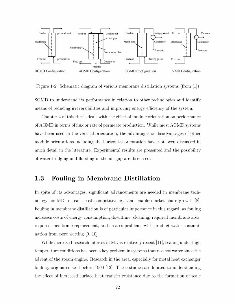
Figure 1-2: Schematic diagram of various membrane distillation systems (from [1])
SGMD to understand its performance in relation to other technologies and identify
means of reducing irreversibilities and improving energy efficiency of the system.
Chapter 4 of this thesis deals with the effect of module orientation on performance
of AGMD in terms of flux or rate of permeate production. While most AGMD systems
have been used in the vertical orientation, the advantages or disadvantages of other
module orientations including the horizontal orientation have not been discussed in
much detail in the literature. Experimental results are presented and the possibility
of water bridging and flooding in the air gap are discussed.
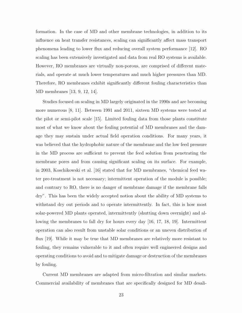
1.3 Fouling in Membrane Distillation
In spite of its advantages, significant advancements are needed in membrane tech-
nology for MD to reach cost competitiveness and enable market share growth [8].
Fouling in membrane distillation is of particular importance in this regard, as fouling
increases costs of energy consumption, downtime, cleaning, required membrane area,
required membrane replacement, and creates problems with product water contami-
nation from pore wetting [9, 10].
While increased research interest in MD is relatively recent [11], scaling under high
temperature conditions has been a key problem in systems that use hot water since the
advent of the steam engine. Research in the area, especially for metal heat exchanger
fouling, originated well before 1900 [12]. These studies are limited to understanding
the effect of increased surface heat transfer resistance due to the formation of scale
22
formation. In the case of MD and other membrane technologies, in addition to its
influence on heat transfer resistances, scaling can significantly affect mass transport
phenomena leading to lower flux and reducing overall system performance [12]. RO
scaling has been extensively investigated and data from real RO systems is available.
However, RO membranes are virtually non-porous, are comprised of different mate-
rials, and operate at much lower temperatures and much higher pressures than MD.
Therefore, RO membranes exhibit significantly different fouling characteristics than
MD membranes [13, 9, 12, 14].
Studies focused on scaling in MD largely originated in the 1990s and are becoming
more numerous [8, 11]. Between 1991 and 2011, sixteen MD systems were tested at
the pilot or semi-pilot scale [15]. Limited fouling data from those plants constitute
most of what we know about the fouling potential of MD membranes and the dam-
age they may sustain under actual field operation conditions. For many years, it
was believed that the hydrophobic nature of the membrane and the low feed pressure
in the MD process are sufficient to prevent the feed solution from penetrating the
membrane pores and from causing significant scaling on its surface. For example,
in 2003, Koschikowski et al. [16] stated that for MD membranes, “chemical feed wa-
ter pre-treatment is not necessary; intermittent operation of the module is possible;
and contrary to RO, there is no danger of membrane damage if the membrane falls
dry”. This has been the widely accepted notion about the ability of MD systems to
withstand dry out periods and to operate intermittently. In fact, this is how most
solar-powered MD plants operated, intermittently (shutting down overnight) and al-
lowing the membranes to fall dry for hours every day [16, 17, 18, 19]. Intermittent
operation can also result from unstable solar conditions or an uneven distribution of
flux [19]. While it may be true that MD membranes are relatively more resistant to
fouling, they remains vulnerable to it and often require well engineered designs and
operating conditions to avoid and to mitigate damage or destruction of the membranes
by fouling.
Current MD membranes are adapted from micro-filtration and similar markets.
Commercial availability of membranes that are specifically designed for MD desali-
23

nation is scarce [11]. Several researchers are actively working on the development
of membranes specially tailored for MD. Understanding the fouling characteristics
of MD membranes under various operating conditions and with the use of different
feed solutions can help improve novel MD membranes, and design systems to operate
under safer conditions.
Chapter 3 describes the construction of an MD experimental setup that can be
used to characterize fouling under well defined feed temperature, flow and salinity
conditions. Experiments conducted with high salinity sodium chloride feed solutions,
as a baseline case to understand the effect of the temperature and concentration
boundary layer resistances are also discussed.
24

Chapter 2
Energy Efficiency of Sweeping Gas
Membrane Distillation Systems
Abstract
Sweeping Gas Membrane Distillation (SGMD) is a carrier gas membrane distillationtechnology that can use low temperature, low grade and waste heat sources and is wellsuited to small scale desalination systems. Understanding the overall thermal effi-ciency, usually in the form of a Gained Output Ratio (GOR), is an important stepits towards commercial implementation. This chapter presents a ‘one dimensional’numerical model of the heat and mass transfer processes in a flat sheet SGMD modulecoupled to a multi-tray bubble column dehumidifier (MBCD). The model is validatedagainst flux data reported in literature. It is used to analyze entropy generation andstudy the effect of various parameters on the efficiency of SGMD desalination cycles.While previous studies have focused on the MD segment and on improving flux, en-tropy generation in both the SGMD module and the dehumidifier can be important andthey both affect the overall cycle efficiency. GOR values in excess of 2.5 are observedin single stage once through SGMD-MBCD desalination cycles.
2.1 Introduction
In membrane distillation (MD), desalination is achieved by passing water vapor
through the pores of a hydrophobic membrane by establishing a temperature-driven
vapor pressure difference between the feed and permeate sides of the module. The
hydrophobicity of the membrane ensures that liquid water does not pass through and
25

thereby ensures almost 100% elimination of non-volatile impurities such as salt in the
permeate. Hot saline water constitutes the feed in these systems. Based on the design
of the permeate side, MD processes have been classified into four major categories -
Direct Contact (DC), Air Gap (AG), Sweeping Gas (SG), and Vacuum (V) MD. [20]
DCMD has a cold pure water stream flowing counter-current to the feed on the
permeate side, onto which the vapor condenses immediately after crossing the mem-
brane. Since the hot and cold streams are separated only by a thin membrane, there
is significant sensible heat transfer. This heat transfer, in addition to being a loss,
also adds to temperature polarization in the streams [21]. AGMD on the other hand
has a cold condensing plate separated from the membrane by a thin layer of stagnant
air. This way, sensible heat loss from the feed is reduced since air has a lower thermal
conductivity. The evaporated water has to diffuse through the air gap and reach the
film of condensate on the cold plate which becomes one of the rate limiting steps.
SGMD has an air stream that flows on the permeate side picking up the incoming
vapor and getting humidified as it moves along the module. Generally the temper-
ature of air also increases along the module. The hot humid air is then cooled in a
condenser where product water is recovered. Although SGMD combines advantages
of both DCMD (lower mass transfer resistance on the permeate side) and AGMD
(lower sensible heat loss across the membrane) configurations, since additional equip-
ment (dehumidifier) is required to condense the product water out of the air stream,
it has received scant attention compared to other types of MD technology, both in
theoretical and experimental studies [1]. Until 2011, only 4.5% of papers related to
MD were on SGMD [11].
With the development of compact, high-effectiveness and low cost dehumidifiers
[22], SGMD has the become more competitive as a means to purify water. Most
literature on MD has focused on improving membrane flux rather than on energy
efficiency (GOR), which is the relevant parameter for comparison with other estab-
lished thermal desalination technologies such as MSF and MED [2]. Therefore, in this
study, we develop a numerical model of the heat and mass transfer processes within a
SGMD module, which is then coupled with a dehumidifier model to form a complete
26

desalination system for efficiency analysis.
2.1.1 SGMD Process
Figure 2-1: Schematic diagram of SGMD process
Figure 2-1 shows a schematic diagram of the SGMD module. The feed stream
and the air stream flow counter-current to each other. The feed inlet temperature is
of the order of Tf,in ≈ 60 ◦C. The air stream generally enters at a lower temperature
of about Ta,in ≈ 25 ◦C. Both heat and mass are transferred from the hot feed side to
the air stream. The temperature and humidity of the air stream increase along the
module whereas the feed cools down before exiting.
The driving force for heat transfer is the difference in temperature (dry bulb
temperature - DBT, for the air stream) between the stream. Mass transfer is driven
by the vapor partial pressure difference between the liquid surface and the air stream.
2.1.2 Bubble Column Dehumidifier (BCDH) Process
In this study we use a multi-tray bubble column dehumidifier (MBCD) as the dehu-
midifier along with the SGMD module to complete the desalination cycle. MBCD has
27

Figure 2-2: Schematic diagram of BCDH process
been proposed as an alternative to conventional dehumidifiers that use large metal ar-
eas for condensation and are therefore quite expensive. Figure 2-2 shows a schematic
diagram of a single stage BCDH. The BCDH is an example of a direct contact dehu-
midifier where a hot moist air stream is bubbled through a column of pure water. The
water vapor from the air bubbles condenses at the bubble surface and releases energy
into the water column. By the time the air leaves the water column, it is cooled
down and leaves close to the temperature of the water column. The heat released by
the condensing vapor is removed from the water column by a coolant stream. In our
system, the inlet saline feed water flowing inside a copper tube acts as the coolant.
The energy released by condensation is therefore recovered and reused for preheating
the feed water. Further discussion on the performance of BCDH compared to con-
ventional dehumidifiers and the effect of high proportion of non-condensible gases is
available in [22].
In Sec. 2.2, the modeling methodology is explained, followed by validation of the
model in Sec. 2.3. Sec. 2.4 has a brief discussion on entropy generation within the
individual components. Finally, results from simulations of the complete desalination
cycle are discussed in Sec. 2.5.
28

2.2 Modeling
The numerical modeling was carried out using the commercial software, Engineering
Equation Solver (EES) [23]. EES is an iterative numerical simultaneous eqution solver
that uses accurate thermodynamic property data for air-water mixtures and water.
The air-water mixture properties in EES are evaluated using formulae presented by
Hyland and Wexer [24] and water properties are evaluated using the IAPWS 1995
formulation [25].
2.2.1 SGMD Module
Method
Khayet et al. [26, 27] have developed theoretical models of the transport processes
within a SGMD module by considering the resistances to heat transfer, namely the
feed and air side boundary layers as well as the membrane. Charfi et al. [28] modeled
the module in two dimensions using the Navier-Stokes equation for both fluid streams
with a suitable coupled boundary conditions at the membrane interfaces.
The modeling approach followed in this work is an extension of the technique
presented in [2] for AGMD, DCMD and VMD systems. A one dimensional model-
ing approach is followed wherein property variations along the length direction are
modeled using suitable conservation equations [29]. The fluid streams are assumed
uniform in the width direction. Along the depth direction the effect of the boundary
layers close to the membrane surface for either stream can not be ignored. These
effects are captured by solving for the fluid properties at the membrane interface for
both streams, and the interface values are also allowed to vary along the flow direction
(length) of the module.
The advantage of this method is that it is computationally less cumbersome com-
pared to a 2D Navier Stokes model. At the same time there is enough detail available
to draw useful conclusions about system performance and to study the effect of various
system variables.
29
Equations
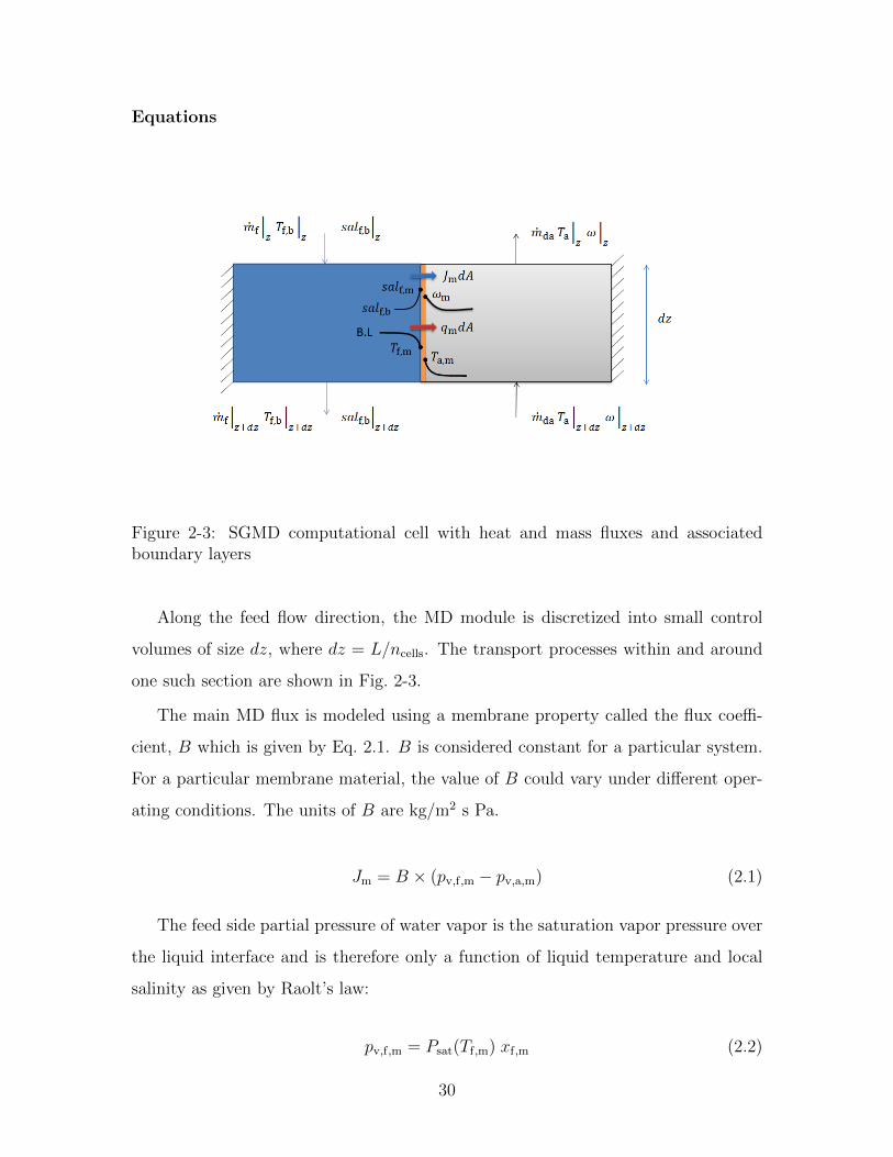
Figure 2-3: SGMD computational cell with heat and mass fluxes and associatedboundary layers
Along the feed flow direction, the MD module is discretized into small control
volumes of size dz, where dz = L/ncells. The transport processes within and around
one such section are shown in Fig. 2-3.
The main MD flux is modeled using a membrane property called the flux coeffi-
cient, B which is given by Eq. 2.1. B is considered constant for a particular system.
For a particular membrane material, the value of B could vary under different oper-
ating conditions. The units of B are kg/m2 s Pa.
Jm = B × (pv,f,m − pv,a,m) (2.1)
The feed side partial pressure of water vapor is the saturation vapor pressure over
the liquid interface and is therefore only a function of liquid temperature and local
salinity as given by Raolt’s law:
pv,f,m = Psat(Tf,m) xf,m (2.2)
30

On the air side, we use the ideal gas relationships to obtain pv,a,m as shown in
Eq. 2.3 and 2.4:
pv,a,m = Paxa,m (2.3)
xa,m =ωm
MWv
ωm
MWv+ 1
MWa
(2.4)
We see that while on the feed side the vapor pressure is a strong function of
temperature, on the air side, temperature of the air stream doesn’t come into the
picture. Most SGMD models [26] assume that the air stream is saturated at the inlet
and remains saturated subsequently. Under those conditions, the partial pressure of
water vapor in the air gap side is also only a function of the air temperature, since
the state of saturated air is completely determined by its temperature. In our model,
we do not make this assumption and hence in general, the partial pressure is not just
a function of air’s DBT.
On the feed side, mass and energy balance equations (Eq. 2.5,2.6) are solved:
mf |z+dz = mf |z − JmdA (2.5)
(mfhf,b) |z+dz = (mfhf,b) |z − (Jmhv,f,m + qm) dA (2.6)
Theoretically, for an internal flow Eq. 2.6 is valid only for bulk temperature defined
as a mass averaged temperature over the cross sectional area of the flow. Here the
equation is used with the value of the temperature outside the boundary layer as an
approximation of the theoretical bulk value.
In addition to the mass flux, there is a heat flux across the membrane governed
by the temperature difference across the membrane and the effective thermal conduc-
tivity of the MD membrane:
qm =keff,m
δm
(Tf,m − Ta,m) (2.7)
31
The value of temperature at the membrane interfaces is determined as a function
of the net heat transfer, heat transfer coefficient and free stream temperature value
(Eq. 2.8, 2.9):
Tf,m = Tf,b − (Jm(hv,f,m − hf,b) + qm)/αf (2.8)
Note that while the entire energy loss from the feed side contributes to the tem-
perature polarization on the feed side, only the sensible heat addition to the air
stream is considered for temperature polarization on the air side. The latent heat
of evaporation does not feature in the temperature polarization expression. Even
under fogging conditions where a small amount of liquid water is formed in the air
stream, the condensation and corresponding energy release is assumed to happen in
the bulk since relative humidity computed at the membrane interface is always less
than 1. The excess thermal energy carried by the vapor and the sensible heat input
are transferred into the vapor stream from the membrane interface by convection:
Ta,m = Ta + (Jm cp,v(Tf,m − Ta)) + qm)/αa (2.9)
The heat and mass transfer coefficients are evaluated using standard correlations
for Nu and Sh for internal flows based on the Re, Pr and Sc numbers of the flow [30].
The salinity at the membrane interface on the feed side is evaluated using the film
model of concentration polarization as
salf,m = salf,b exp
(Jm
kmass,f ρf
)(2.10)
Air Stream
In Eq. 2.4, we saw that the vapor partial pressure depends on the humidity ratio at
the membrane interface. This is evaluated again using the film model as
ρ(
11+ω
)ρm
(1
1+ωm
) = exp
(Jm
kmass,a ρa
)(2.11)
32

Mass and energy balance equations are solved on the air gap side as well:
mda (ω|z − ω|z+dz) = JmdA (2.12)
mda(ha|z − ha|z+dz) = Jmhv,f,mdA+ qmdA (2.13)
When EES solves the above equations based on the mass and energy fluxes that
enter the air stream, since the air-water mixture enthalpy function in EES is defined
even for supersaturated states (relative humidity > 1), a check needs to be placed on
whether supersaturation occurs. Whenever the air stream tends to become supersa-
tured with water, the state of air is forced back to the saturation line at the same
enthalpy in order to simulate fogging. Any excess water after this is done, is assumed
to be in the liquid state as fog carried forward by the air stream.
The local entropy generation for the control volume located between z and z+dz is
evaluated to make sure that the second law of thermodynamics is satisfied everywhere
locally.
2.2.2 Multi-tray Bubble Column Dehumidifier
Figure 2-4 shows a schematic diagram of a multi-tray bubble column dehumidifier.
Hot moist air is bubbled through a series of water columns (stages), which are cooled
by cool feed water. The condensed moisture from each stage is added to a subsequent
stage and finally water at the lowest temperature (from stage 1) is extracted as pure
product. Air leaves saturated at a temperature close to the that of the water column
in each stage in a well designed BCDH. The water stream also gets heated to a
temperature slightly below the temperature of water column. This is illustrated in
Fig. 2-5. The difference in temperature between the air and coolant that leave a stage
is called the terminal temperature difference (TTD) of the stage.
The main goal of the present study is to model the SGMD module in detail. Tow
and Lienhard [31] have reported data from several bubble column dehumidifier ex-
periments. Based on that data, a TTD of 1 ◦C is assumed for each stage of a well
33

Figure 2-4: Schematic diagram of MBCD system with four stages
designed MBCD. In addition to this imposed condition, first law and mass conserva-
tion are solved for each stage and the stages are coupled together in order to solve
for the overall outputs of the dehumidifier.
2.3 Validation
Charfi et al. [28] have published flux data from experiments conducted on a flat sheet
SGMD module. Based on the data reported, the geometry of the experimental setup
is estimated and programmed into the one dimensional model.
While the physical properties of the membrane such as porosity, mean pore size,
and tortuosity have been reported, no value of membrane distillation mass transfer
34

Figure 2-5: Temperature vs. position for a MBCD system showing the terminaltemperature difference (TTD)
coefficient B is mentioned. The B value was fixed at 1.7 × 10⁻⁷ kg/m2 s Pa a good
match between the 1D model simulation results and experimental data is obtained.
(Fig. 2-6).
Though additional experimental measurements are not included in the reference,
simulation results from the 2D model are discussed. The overall match between
experiment and the simulation has also been reported to be quite good (R2 = 0.9406).
The baseline conditions of their experiments and important physical parameters are
collected in Tab. 2.1. Similar simulations are carried out using the one dimensional
model described here.
The corresponding results from our model, at the same value of B determined
earlier are included in Fig. 2-7. The flux decreases with an increase in air temperature
since the inlet air stream was maintained at a saturated state in the experiment. As
a result, an increase in temperature of the air meant a corresponding exponential
increase in vapor partial pressure in the air and hence a reduction in the net driving
force for mass transfer.
The SGMD flux increases with an increase in air stream velocity (Fig. 2-7(b))
since a higher air mass flow rate implies quicker vapor removal by the air stream. At
very low air mass flow rates, the air stream is effectively humidified and heated close
35
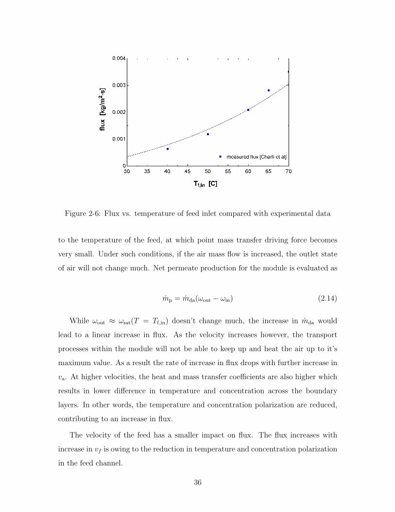
Figure 2-6: Flux vs. temperature of feed inlet compared with experimental data
to the temperature of the feed, at which point mass transfer driving force becomes
very small. Under such conditions, if the air mass flow is increased, the outlet state
of air will not change much. Net permeate production for the module is evaluated as
mp = mda(ωout − ωin) (2.14)
While ωout ≈ ωsat(T = Tf,in) doesn’t change much, the increase in mda would
lead to a linear increase in flux. As the velocity increases however, the transport
processes within the module will not be able to keep up and heat the air up to it’s
maximum value. As a result the rate of increase in flux drops with further increase in
va. At higher velocities, the heat and mass transfer coefficients are also higher which
results in lower difference in temperature and concentration across the boundary
layers. In other words, the temperature and concentration polarization are reduced,
contributing to an increase in flux.
The velocity of the feed has a smaller impact on flux. The flux increases with
increase in vf is owing to the reduction in temperature and concentration polarization
in the feed channel.
36
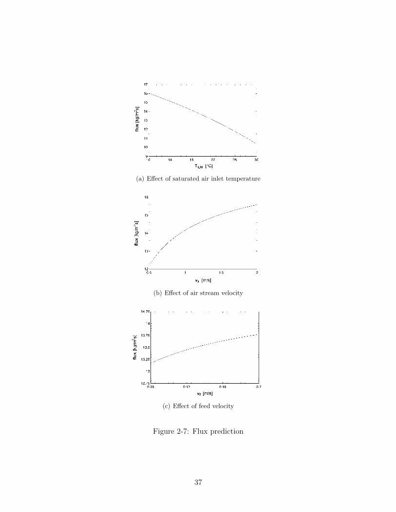
(a) Effect of saturated air inlet temperature
(b) Effect of air stream velocity
(c) Effect of feed velocity
Figure 2-7: Flux prediction
37

Table 2.1: Baseline values for validation test cases
S No Variable Value Units1 Tf,in 50 ◦C2 Ta,in 20 ◦C3 vf 0.15 m/s4 va 0.8 m/s5 salin 0 ppt6 L 0.068 m7 w 0.08235 m8 df , da 0.005 m9 B 1.7× 10⁻⁷ kg/m2 s Pa
Comparing with corresponding graphs from the 2D model (Fig. 5,7,8 of [28]), we
see that the trends predicted by the two dimensional model are captured accurately
by the present model. The absolute value of flux differs between the two models by
a maximum of about 20%.
2.4 SGMD and MBCD System Analysis
2.4.1 Entropy Generation and GOR
The efficiency of a thermal desalination cycle is given by the Gained Output Ratio
(GOR), a measure of the extent to which the supplied heat energy is reused within
the system for evaporation and purification of the feed. GOR is defined as
GOR =mphfg
Qin
(2.15)
In this paper, hfg for GOR evaluation is taken at 25 ◦C since MD uses low grade,
low temperature heat sources. Other publications may use the value of hfg at 100 ◦C.
Since hfg(100◦C) = 2.257× 10⁶ J/kg and hfg(100◦C) = 2.442× 10⁶ J/kg, a GOR of
2.6 reported here would correspond to GOR=2.8 if enthalpy of vaporization at Tbp is
used.
For desalination systems, it has been shown that minimizing specific entropy gen-
38
eration (sgen is entropy generated per unit rate of permeate production) results in
maximum GOR [5]. The entropy generation characteristics of the SGMD and MBCD
systems are analyzed separately before they are put together to form a complete
desalination system.
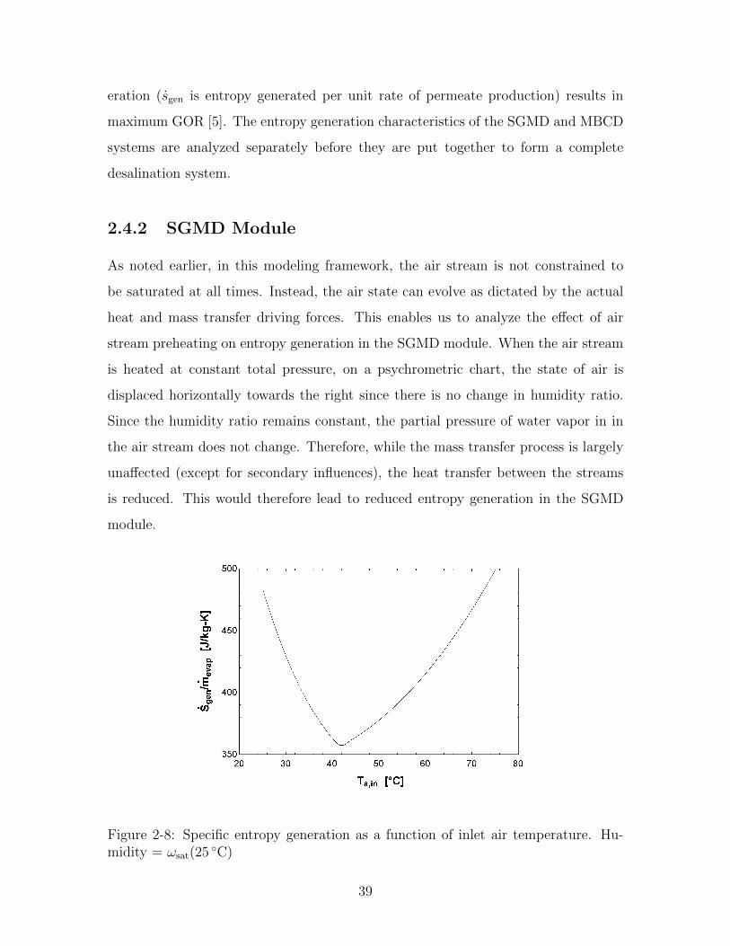
2.4.2 SGMD Module
As noted earlier, in this modeling framework, the air stream is not constrained to
be saturated at all times. Instead, the air state can evolve as dictated by the actual
heat and mass transfer driving forces. This enables us to analyze the effect of air
stream preheating on entropy generation in the SGMD module. When the air stream
is heated at constant total pressure, on a psychrometric chart, the state of air is
displaced horizontally towards the right since there is no change in humidity ratio.
Since the humidity ratio remains constant, the partial pressure of water vapor in in
the air stream does not change. Therefore, while the mass transfer process is largely
unaffected (except for secondary influences), the heat transfer between the streams
is reduced. This would therefore lead to reduced entropy generation in the SGMD
module.
Figure 2-8: Specific entropy generation as a function of inlet air temperature. Hu-midity = ωsat(25 ◦C)
39

Figure 2-8 shows this effect. The entropy generation within the module reduces
and increases again with increase in inlet air DBT. The rate of decrease in entropy
generation is very steep because of air state hitting the saturation dome and fogging
occurring within the stream. The process path traced by the sweeping gas in the
case of two inlet air temperatures (40 ◦C, 50 ◦C) is depicted on a psychrometic chart
in Fig. 2-9. In Fig.2-9(a), the air stream gets heated and humidified until it hits
the saturation dome. Thereafter, as discussed in Sec. 2.2.1, the air state is manually
forced to follow the saturation dome. Total specific enthalpy of the air is used to
choose the point along the saturation line. A small amount of liquid water is formed
whose enthalpy is ignored while determining the air state (hv � hl), but the quantity
of liquid water/fog is calculated and carried forward along with the air stream.
In Fig. 2-9(b) on the other hand, the air is seen to be almost exclusively humidi-
fied(the state of the air stream evolves vertically upward). Initially the air loses DBT
as some heat transfer occurs to the water stream which is at a lower temperature. In
the latter part of the of module, the air is heated and humidified by the feed stream.
The flow evolution along the length of the module can be visualized better using
the help of a temperature vs. position plot. In Fig. 2-10(a), we see that the water
DBT denoted by Ta does not vary much initially as it flows from L = 12 m to about
2 m. At this point, the air stream becomes saturated and it starts following the
saturation curve with Ta = Twb. On the other hand, in Fig. 2-10(b), while the DBT
does not change over the length of the module, the wet bulb temperature increases
steadily.
In both the graphs, the temperatures of the air and feed at the membrane interface
are almost equal. This shows that there is significant temperature polarization in both
streams. Another effect of this is that there is very little sensible heat transfer from
the feed to sweeping gas (qm ≈ 30-40 W/m2). Any sensible heat transfer, in MD is
considered a loss. Interestingly, while the high air side temperature polarization adds
a thermal resistance within the stream, it is beneficial in reducing the net sensible
heat loss from the feed.
Figure 2-11 shows the vapor pressure difference across the membrane which drives
40
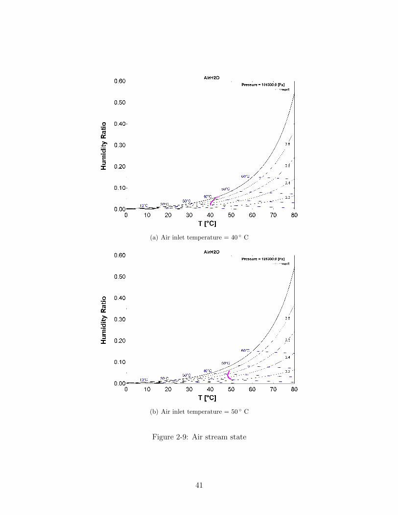
(a) Air inlet temperature = 40 ◦ C
(b) Air inlet temperature = 50 ◦ C
Figure 2-9: Air stream state
41

(a) Air inlet temperature = 40 ◦C
(b) Air inlet temperature= 50 ◦C
Figure 2-10: Temperature vs. position
42

transfer of pure water vapor. As explained earlier, the increased DBT of the inlet
air does not affect the vapor pressure of the air stream and hence the mass transfer
processes in the two cases are nearly identical. In Fig. 2-11(b), we see that in the
lower specific entropy production case, the air stream vapor pressure at the exit is
slightly higher indicating a small increase in overall flux. These graphs characterize
the physical processes within the module and help confirm that the model captures
the phenomena accurately.
2.4.3 Multi-tray Bubble Column Dehumidifier
The specific entropy generation in the proposed MBCD model is plotted in Fig. 2-12.
As expected, the specific entropy generation has a minima with respect to changing
mda with other parameters fixed. Combined heat and mass transfer devices such as
dehumidifiers (and humidifiers) produce minimum entropy when the heat capacity
rates of the two streams are matched [32].
The irreversibility within the device increases with increase in Ta,in,BCDH under
these conditions [2-12(b)]. This is expected since with an increase in inlet air tem-
perature, both heat and mass transfer driving forces increase in the system.
2.5 Cycle Analysis
A schematic diagram of the overall desalination cycle is illustrated in Fig. 2-13. The
two models are combined by matching their inlet and outlet states suitably in EES.
The configuration chosen is a closed air open water configuration. Cold water is
taken into the dehumidifier and used to as the coolant. As it passes through, the
enthalpy of condensation is transferred from the water column into the cold water
stream and it is preheated. The feed water then goes through a water heater where
it is heated to the cycle top temperature. In this study, the cycle top temperature
is fixed and hence the heat input varies depending on the extent of preheating. The
hot water then goes through the SGMD module. Here evaporation causes cooling
of the feed. The minimum temperature to which the feed can get cooled is the wet
43

(a) Air inlet temperature = 40 ◦C
(b) Air inlet temperature = 50 ◦C
Figure 2-11: Vapor pressure vs. position
44

(a) Effect of mda
(b) Effect of Ta,in,BCDH
Figure 2-12: Specific entropy generation in a MBCD. (Ta,in = 50 ◦C, mc= 0.189 kg/s,Tc,in= 25 ◦C)
45

bulb temperature of the air inlet into the SGMD module and as it approaches this
temperature the driving force for mass transfer will reduce. The brine that exits the
SGMD module is disposed.
The air stream forms a closed loop as the name of the configuration indicates.
Air enters the SGMD module and is humidified by addition of vapor from the feed
stream. In the process, the temperature of the air also increases. This stream is
then taken into the MBCD where it is bubbled through multiple water baths using
spargers. As the bubbles rise, air is cooled and excess water vapor condenses into the
water. The air that exits the MBCD is then fed back into the SGMD module.
Since the two devices are now coupled, the number of degrees of freedom is re-
duced. The temperature of the air stream is no longer an input to the system. The
mass of the liquid streams are also equal in both the devices. We previously observed
that sgen is minimized in the MBCD at a particular value of mr = mda/mf . Similarly
the SGMD system would produce minimum entropy at a different value of mr. Since
the entropy generation in both devices is of the same order of magnitude, the over-
all system performance and the effect of the system inputs would be a result of the
combined effect of both devices.
The baseline parameters for the simulations are given in Table 2.2. Each of the
parameters are varied around their baseline value keeping the other variables constant
to understand their effect on the overall cycle GOR.
2.5.1 Mass Flow Rates
The mass flow rates are important parameters in the SGMD desalination system.
With both the SGMD module and the MBCD irreversibilities being functions of mr,
the overall system too is very sensitive to the mass flow rates of feed and air. In
addition to its effect on the thermodynamics as described above, the mass flow rate
of a stream also affects the Reynolds number and thereby the Nusselt and Sherwood
number of the stream in the SGMD module. Through its effect on the Nu and Sh,
an increase in mass flow rate of either stream would lead to a monotonic increase in
GOR of the cycle. The thermodynamic effect dominates as is seen in Fig. 2-14, with
46

Figure 2-13: Complete SGMD-MBCD desalination system
the GOR attaining a maximum at a particular value of feed and air mass flow rate
and reducing thereafter.
2.5.2 Temperatures
SGMD feed inlet
The temperature of the feed input the SGMD module is a design variable and is the
cycle’s top temperature. Figure 2-15 shows the effect of cycle top temperature on
GOR. When all other parameters such as system geometry and flow rates are fixed,
GOR is maximized at Tf,in = 70◦ C.
47

(a) Feed side. Discontinuity due to transition to turbulence
(b) Air side
Figure 2-14: GOR dependence on mass flow rates
48

Table 2.2: Baseline values of SGMD desalination system
S No Variable Value Units1 Tf,in 60 ◦C2 Tcold,w,in 25 ◦C3 mf,in 0.189 kg/s4 mda 0.1345 kg/s5 salf,in 30 ppt6 L 12 m7 w 0.125 m8 df 0.004 m9 da 0.04 m10 B 16× 10−7 kg/m2 s Pa11 TTD 1 ◦C12 nBCDH,stages 6 -
Coolant
The temperature of the coolant (feed inlet from the environment) has a smaller effect
on GOR (Fig. 2-16). Since the baseline mass flow rates were chosen such that GOR
is maximized, the GOR is maximum close to Tc,in = 25 ◦C.
2.5.3 Geometry
Geometry of the SGMD module affects the transport processes within significantly.
Figure 2-17 shows the influence of the effective length and width of the module on
GOR. Both length and width affect the total available membrane area. While the
length does not affect the cross section and hence the flow velocity, changing the width
introduces these additional effects as well. At the baseline operating parameters and
module dimensions (chosen to be in the range of other commonly studied MD systems
[2]), the SGMD module design is not optimized since Tf,out from the module is much
higher than the wet bulb temperature of the air inlet (see Fig. 2-10, for example).
Increasing the area of the membrane is similar to increasing the area of a heat ex-
changer. The total heat and mass transfer increase and the overall irreversibility in
the system decreases with an increase in both width and effective length.
49

Figure 2-15: GOR dependence on cycle top temperature
Figure 2-17(a) shows that increasing the length of the module results in a large
increase in GOR. With the flow characteristics and mass flow ratios unaltered, the
increase is predominantly owing to better usage of the heat in the feed stream. With
increase in length, Tf,out decreases and the mass transfer occurs over a smaller ∆pv.
In Fig. 2-17(b), the gap in the graph corresponds to a change of feed flow regime
to laminar as the cross sectional area increases with increase in width. The GOR
increase is observed over a smaller range in the case of width as compared to length.
This is because of the other being held constant. When the width is increased to 3 m,
the length is held constant at 12 m resulting in an overall membrane area of 36 m2.
On the other hand, to reach the same membrane area with a width of 0.125 m, the
length must be 144 m. Note that at an effective length of 144 m, the GOR achieved
is higher than at width of 3 m though the overall membrane area is the same. This is
because an increase in length does not affect the flow regime in the module and the
feed and air Reynolds numbers remain the same (Ref ≈ 5000,Rea ≈ 4.4 × 10⁴). On
the other hand, the Reynolds numbers and hence heat and mass transfer coefficients
of both streams reduce with an increase in width. In a real system one would have to
50

Figure 2-16: GOR dependence on cycle bottom temperature
pay for the increased GOR in the longer module in the form of a much larger pressure
drop and hence pumping power, compared to the wider module which has a slightly
lower GOR.
The effect of the depth of the two channels is illustrated in Fig. 2-18. The effect
of increasing d is similar for both the streams. The membrane area remains unaltered
and the only effect is on cross sectional area and therefore on the transport processes
and boundary layers in the two streams. Correspondingly, the change in GOR over the
range of df and da is smaller than in the case of the other dimensions. An increase
in depth of the channel leads to higher boundary layer resistances and therefore
smaller GOR. Figures 2-18(a) and 2-18(b) suggest that polarizations in both streams
are significant. The temperature polarization in the feed stream and concentration
polarization in the air stream have maximum impact since they directly affect the
mass transfer driving force by reducing the vapor pressure difference substantially.
The concentration polarization on the feed side can have a significant effect too,
especially under laminar flow conditions.
51

(a) Effective length
(b) Width
Figure 2-17: GOR dependence on length and width
52

(a) Feed side
(b) Air side
Figure 2-18: GOR dependence on channel depth
53

2.5.4 Dehumidifer Effectiveness
MBCD effectiveness increases with number of stages. The number of stages also
determines the pressure drop through the system and the cost. The marginal gains
in GOR with increase in the number of stages of the dehumidifier is presented in
Fig. 2-19.
Figure 2-19: Effect of number of BCDH stages
2.5.5 Membrane Properties
The B value of the membrane directly influences the flux in MD processes. With
higher B giving rise to higher flux, one could use smaller devices. In other words, if
the membrane area is held constant and the membrane permeability is increased, we
can expect to see an increase in efficiency as shown in Fig. 2-20. It should be noted
that higher permeability alone does not guarantee good thermal efficiency (GOR vs.
B graph plateaus beyond a point). While high permeability membranes will help,
they are not a substitute for thermodynamic analysis and cycle design.
54

Figure 2-20: Effect of membrane permeability
2.5.6 Further Improvements
In the preceding sections, the effect of each independent variable was studied keeping
other parameters fixed. This yields a GOR just over 2 with large enough membrane
area (≈ 36 m2). Further improvements to GOR are possible when all the independent
variables are allowed to change. For example, Fig. 2-21 shows the effect of feed mass
flow rate on GOR when the module effective length is set as 60 m. The maximum
GOR attained is close to 2.6 in this case.
2.6 Conclusions
A one-dimensional numerical model of the heat and mass transfer processes occurring
in a SGMD module is developed. The model can take in both saturated and unsatu-
rated air as input and the process path is evaluated using the membrane distillation
coefficient B. Entropy generation within the SGMD module is studied with respect
to changes in the system variables.
The model has been used to study the energy efficiency of the SGMD based de-
salination cycle using a multi-tray bubble column dehumidifier to recover pure water.
55

Figure 2-21: GOR vs. feed mass flow rate. L = 60 m
Entropy generation in the dehumidifier is found to be important, often competing
with the SGMD module in deciding the optimum operating conditions.
The boundary layer resistances and associated temperature/concentration polar-
izations are found to have a significant impact on reducing thermal efficiency. Im-
provements in mixing within the streams such as the use of suitable spacers of baffles
can lead to further improvements in efficiency.
This model can be a useful tool for designing optimal desalination cycles under a
set of design constraints. The effect of each independent variable on GOR was studied.
For a longer module, a maximum GOR in excess of 2.5 is observed with changing
feed mass flow rate. Now that the effect of each individual process parameter is
understood, further optimization is possible to look for operating conditions that
yield global maximum GOR.
56

Chapter 3
Experimental Design of Air Gap
Membrane Distillation System for
Fouling Tests
David E. M. Warsinger contributed to this chapter.
Abstract
Experimental investigation of inorganic salt fouling in MD is a useful tool to mapregions of safe operation where MD can be used over long periods of time. In relationto this, the experimental design of an air-gap membrane distillation apparatus withwell defined feed thermal, concentration and flow conditions is described in this chap-ter. The desirable features of each component of the experimental setup are discussedand solutions to practical challenges faced during the experiments are illustrated. Ex-periments were conducted over a wide range of temperature, flow rate and NaCl feedsalinity conditions. Theoretical modeling of the heat and mass transport processes wasable to successfully predict the dependence of flux on system input parameters. Thismodel can therefore be used in the future to design specific membrane fouling testswith known conditions at the fluid membrane interface.
3.1 Introduction
One of the frequently quoted beliefs about the membrane distillation desalination
process is its relatively higher resistance to fouling [33]. Membrane distillation being
57

a thermally driven technology has very high potential in the market for treatment of
high salinity feed streams where reverse osmosis cannot be used [34]. Under these
conditions, the importance of fouling resistance becomes multi-fold. Characteristic
high salinity feed solutions include RO brine solutions at about 70 ppt salinity and
hydraulic fracturing flow back water that span a wide range of composition and
salinities. In industrial operation MD membranes are likely to be exposed to several
types of potential foulants including organic, inorganic and biological substances. Of
these, inorganic crystalline precipitation scaling is relatively better understood in
other engineering systems and especially in other membrane systems [9].
Quantifying fouling characteristics of various salts under membrane distillation
process operating conditions will be extremely useful in finding out safe operating
regimes for a given feed stream composition. Knowing the rate of fouling and related
flux decline, we can better estimate cleaning frequency and costs when designing sys-
tems. The efficiency of anti-foulants and cleaning methodologies can also be studied
in a targeted and scientific manner using such an experimental apparatus.
3.2 Design Criteria
In any real MD system, the feed stream would start off relatively dilute and will get
progressively concentrated as it loses pure water. As a result, a common observation
in RO and other systems is that the far end of the membrane is more susceptible to
inorganic fouling and this is likely to be true in MD as well. In order to be able to test
the fouling conditions under a wide variety of well characterized operating conditions
though, it is challenging to use a realistic MD system since the internal dynamics of
temperature and concentration along the length of the module can only be, at best,
estimated using analytical or numerical models of the system operation. On the other
hand, we want to generate a map of temperature and concentration conditions and
corresponding potential foulants in MD, wherein it is important to know with some
degree of certainty the actual conditions at the membrane area of interest.
In order to satisfy these requirements, a small scale MD setup is chosen (Fig. 3-1).
58

Since the effective membrane area is small, the feed flow rate, temperature and salinity
do not really vary by much from the inlet to the outlet of the module. Measured rate
of fouling in such a system would correspond to a local region along the feed flow
direction in a large scale system. By changing the three variables independently it
is possible to map the whole domain of temperature, salinity and flow rates and
therefore infer the local fouling rates in a real setup.
Figure 3-1: A schematic diagram of the MD experimental setup
3.2.1 Module Type
Several MD module configurations have been designed and tested, including plate
and frame, spiral wound and hollow fiber designs. Of these, the plate and frame
design is the most frequently implemented and has been chosen for this study as well.
This configuration is the easiest to build at the lab scale with flat membranes being
available on the market that can be used directly. Observing scale in situ is easier on
a flat membrane that is directly accessible and can be visualized from outside. Plate
59

and frame also allows for easy removal, cleaning and replacement of membrane which
is an essential feature of a fouling analysis experiment [35].
3.2.2 MD Configuration
Several types of MD systems have been studied, including the direct contact, air
gap, sweeping gas and vacuum or reduced pressure systems based on the design of
the permeate side of membrane. Summers et al. [2] have analyzed these single stage
systems and evaluated their performance in terms of energy recovery. AGMD modules
were shown to have highest potential for optimization and high energy efficiencies, as
shown in Fig. 3-2 where for equal membrane area, at large effective lengths, the GOR
of AGMD exceeds both that of DCMD and VMD configurations.
Figure 3-2: GOR comparison between single stage MD configurations [2]
There are other advantages that AGMD enjoys over DCMD. In AGMD, the pro-
duced pure water stream is collected independent of the cooling water, whereas in
DCMD, the product water condenses directly into the cooling water stream. As a
result, product water flux can be measured directly and with much better accuracy in
AGMD. Leakage through the membrane can also be detected earlier since an increase
60

in salinity of the collected permeate is observed immediately, whereas in DCMD the
salt water that leaks will get diluted by the pure cold water.
3.2.3 Feed Reynolds Number
MD studies in the literature are carried out over a wide range of flow rate conditions.
The Reynolds number of the feed flow is an important variable in more ways than
one. The flow condition being laminar or turbulent is a function of the Reynolds
number and would control the heat and mass transfer coefficients within the channels
and correspondingly the extent of temperature and concentration polarization. In
practice it is likely that systems would run at slightly turbulent conditions to make
use of the membrane area quite effectively, by reducing the boundary layer resistances.
In addition to affecting the transport properties, the velocity of fluid flow within
the module also plays a role in the kinetics of the scaling process. Inorganic fouling is
considered to be a sequential process where a seed of fouling material attaches to the
membrane, followed by growth of crystals. Crystals may be sheared off by the flow,
and the balance between the growth and removal processes defines an equilibrium
condition for fouling. High flow rates are likely to increase the rate of scale removal
from the membrane surface [36].
The feed flow channel has a depth of 4 mm. The Reynolds number can be varied
from about 1000-5000 in our experiment with a corresponding feed average velocity
range of 0.06-0.66 m/s.
3.2.4 Membrane Area
We use a 16 cm by 12 cm area of active membrane. The total active area of membrane
used is important since under fixed temperature conditions, the flux is linearly related
to the effective membrane area.
J = B ×∆Pvap × A (3.1)
The relative error in flux measurement would decrease at high values of absolute
61
water production. Since flux decline is one of the most commonly used metrics to
infer fouling, measuring flux with higher accuracy is desirable. As a result, we use a
larger membrane area than is used in many other coupon type test setups [37].
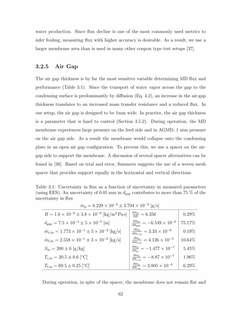
3.2.5 Air Gap
The air gap thickness is by far the most sensitive variable determining MD flux and
performance (Table 3.1). Since the transport of water vapor across the gap to the
condensing surface is predominantly by diffusion (Eq. 4.2), an increase in the air-gap
thickness translates to an increased mass transfer resistance and a reduced flux. In
our setup, the air gap is designed to be 1mm wide. In practice, the air gap thickness
is a parameter that is hard to control (Section 3.5.2). During operation, the MD
membrane experiences large pressure on the feed side and in AGMD, 1 atm pressure
on the air gap side. As a result the membrane would collapse onto the condensing
plate in an open air gap configuration. To prevent this, we use a spacer on the air-
gap side to support the membrane. A discussion of several spacer alternatives can be
found in [38]. Based on trial and error, Summers suggests the use of a woven mesh
spacer that provides support equally in the horizontal and vertical directions.
Table 3.1: Uncertainty in flux as a function of uncertainty in measured parameters(using EES). An uncertainty of 0.05 mm in dgap contributes to more than 75 % of theuncertainty in flux
mp = 8.229× 10⁻² ± 3.794× 10⁻³ [g/s]
B = 1.6× 10⁻⁶ ± 3.8× 10⁻⁸ [kg/m2 Pa s] ∂mp
∂B= 6.356 0.29%
dgap = 7.5× 10⁻⁴ ± 5× 10⁻⁵ [m] ∂mp
∂dgap= −6.549× 10⁻² 75.17%
mc,in = 1.773× 10⁻¹ ± 5× 10⁻² [kg/s] ∂mp
∂mc,in= 3.33× 10⁻⁶ 0.19%
mf,in = 2.558× 10⁻¹ ± 3× 10⁻² [kg/s] ∂mp
∂mf,in= 4.126× 10⁻⁵ 10.64%
Sin = 200± 6 [g/kg] ∂mp
∂Sin= −1.477× 10⁻⁷ 5.45%
Tc,in = 20.5± 0.6 [◦C] ∂mp
∂Tc,in= −8.87× 10⁻⁷ 1.96%
Tf,in = 69.5± 0.25 [◦C] ∂mp
∂Tf,in= 3.805× 10⁻⁶ 6.29%
During operation, in spite of the spacer, the membrane does not remain flat and
62

at a fixed distance from the condensing plate. The membrane is pushed into the gaps
in the air gap spacer due to hydraulic pressure and this reduces the effective air gap
thickness, as seen in Fig. 3-3. In addition, conduction across the plastic spacer and
the spacer’s effect on the condensate film forming on the plate may also be important.
As a result, this is one of the most difficult parameters to estimate accurately while
modeling the system. The effective air gap width is smaller than the design value for
these reasons and is taken to be 0.75 mm in the modeling analysis.
Figure 3-3: MD membrane during operation: regions of the membrane are pushedinto the gaps in the mesh spacer
3.2.6 Feed, Cold Water
The feed and cold water form a closed loop flowing from large tanks that act as a
thermal reservoirs that ensure relative stability in temperature values over time. The
feed water flows through instrumentation that records its flow rate and temperature,
into the feed module and back into the tank. The feed water temperature is con-
trolled at a set high temperature (40-70 ◦C using a resistance immersion heater and
a feedback controller.
The cold side tank on the other hand often needs to be cooled to maintain its
temperature as it takes up the heat of condensation within the module during op-
eration. The building cold water supply line is used for this purpose and a solenoid
valve is activated to allow cold water flow into a copper tube that is immersed into
63

the water in the tank, whenever the tank temperature rises beyond a set value.
3.2.7 Module assembly
The apparatus is designed in a modular way with separate pieces individually defining
each of the flow channels or segments. These are then held together by bolts that
line all fours sides of the module. The channel sealing is an important feature for
reliable operation. O-rings are used for this purpose, wherever a fluid stream needs
to be confined within a given area.
The module is made up of the feed plate, MD membrane, plastic spacer, air gap
mesh, metal condensing plate, and cooling channel plate (Fig. 3-4).
Figure 3-4: MD assembly showing individual components. Left to right: Metal flange,feed plate, MD membrane, plastic spacer with mesh spacer, condensing plate andcooling channel
Most of the pieces of the design and especially the feed plate are manufactured out
of transparent polycarbonate. Polycarbonate has several useful properties that makes
it an ideal choice. It has a low thermal conductivity, leading to lower heat loss from
the module, which is especially important at high temperature runs. In addition, we
chose a transparent material that enables visual inspection of the membrane surface
64

during the course of the experiment which is useful for the fouling experiments in
particular. In real systems, the low cost of plastics as compared to metals is also
a driver towards their use in MD installations since lower capital costs are are an
important advantage of MD over other systems.
While other experimental setups of this kind have used bolts and nuts to secure
the pieces of the module together, for a scaling test setup, easy removal of membrane
for inspection and changing membranes is a useful feature. While all the other plates
are held together by bolts, the feed plate is held down by a set of specially designed
clamps that can be quickly released or fastened that help hold plate in place and
press it onto the o-ring. Figure 3-5 illustrates this design in the actual experiment.
Figure 3-5: Design of quick release clamps for easy access to membrane between tests
The air gap defining plastic spacer is also made of polycarbonate, and is designed
to be 1 mm thick sheet. This corresponds to the design specification of the air gap.
Several versions of the air gap mesh spacer were tried out before deciding to use
the version shown in Fig. 3-6. Here there are two spacers used. The larger one is a
woven mesh spacer and is placed in contact with the metal plate. In the woven air gap
spacer, the 60-80% of the horizontal elements are removed to minimize interference
with the film of condensate that forms on the plate. On top of this, a much thinner
uniform mesh is used to reduce the stretching of the membrane material into the large
gaps in the large mesh.
The condensing plate used is made of aluminum. With a high thermal conductivity
65

Figure 3-6: A thinner spacer stacked over the woven mesh in the air-gap
and relatively high fouling resistance due to the formation of a protective oxide layer
on its surface, it is suited to an application where it is expected to be in continuous
contact with pure water over long periods of time. During experiments it was found
that while this is predominantly true, it is possible that some of the Al is leached out
by the DI water due to its high level of purity.
The cold side channel is made of polycarbonate too. The channel depth is designed
to be higher than that of the feed side so that the pressure drop is smaller and a smaller
pump can be used on this side. In several real systems (AGMD, DCMD) the cold
side fluid would be the feed getting preheated by the condensing permeate before it
is heated to the cycle top temperature. Since this module was designed especially for
fouling testing and the cold fluid temperature was expected to be kept constant during
the course of the experiment and capable of being modified independently, it could
be designed differently with different dimensions and flow rates as compared to the
hot fluid channel. The pressure plenum and the manifold design were also eliminated
in the cold side, since flow redistribution is of less importance. The aluminum plate
being quite conductive, gets cooled uniformly by the flow.
The o-rings used in this setup are made of Viton material [39]. Standard o-ring
66
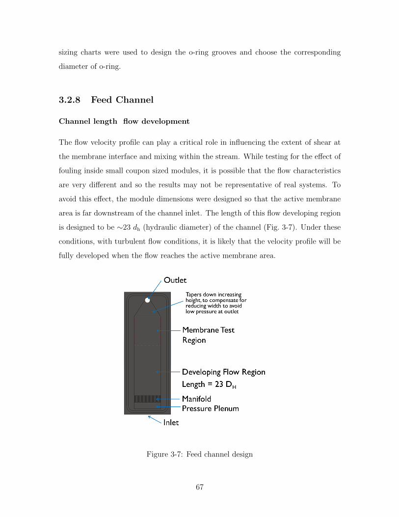
sizing charts were used to design the o-ring grooves and choose the corresponding
diameter of o-ring.
3.2.8 Feed Channel
Channel length flow development
The flow velocity profile can play a critical role in influencing the extent of shear at
the membrane interface and mixing within the stream. While testing for the effect of
fouling inside small coupon sized modules, it is possible that the flow characteristics
are very different and so the results may not be representative of real systems. To
avoid this effect, the module dimensions were designed so that the active membrane
area is far downstream of the channel inlet. The length of this flow developing region
is designed to be ∼23 dh (hydraulic diameter) of the channel (Fig. 3-7). Under these
conditions, with turbulent flow conditions, it is likely that the velocity profile will be
fully developed when the flow reaches the active membrane area.
Figure 3-7: Feed channel design
67

Pressure plenum design
The channel inlet needs to be designed such that irrespective of the velocity profile
in the inlet pipes and the placement of the inlet with respect to the channel, flow
is well distributed across the entire cross section. We followed the guidelines for
Uniform Flow in Dividing Manifolds in [40] to ensure that the pressure drop across
the manifold outlets is an order of magnitude more than that in the water collection
region. The water as it enters the module hits a wall and is forced to recirculated and
fill the high pressure collection chamber before flowing out of the small and equally
spaced outlets at relatively uniform speeds. Figure 3-8 illustrates the design in further
detail.
Figure 3-8: Design of inlet manifold with high pressure reservoir and outflow nozzlesfor uniform outflow. All dimensions are in mm
3.2.9 Membrane
The membranes used are hydrophobic Immobilon-PSQ Membranes [41], originally
designed for protein binding, but have characteristics suitable for Membrane Distil-
68

lation. The membranes have an average pore size of 0.2 µm and maximum of 0.71
µm, and a porosity of 79.2%. They have previously been examined as the principal
membrane used by Dr. Edward Summers at MIT [38].
3.2.10 Piping and Pumps
Magnetic drive pumps were chosen for both the feed [42] and cold [43] fluid loops.
The magnetic drive pumps have no metallic parts that come in contact with the liquid
thereby reducing chances of fouling. The piping is chosen to be flexible clear PVC
tubing for the most part. Before and after the flow meter a small section of hard
CPVC is used since the flow meter accuracy is guaranteed only with a long enough
entrance and exit region.
3.3 Instrumentation
3.3.1 Temperature
Thermistors [44] are used for temperature measurement to achieve ±0.2 ◦C or better
accuracy in the temperature readings. Thermistors were calibrated over a range of
temperatures (0-80 ◦C) using a constant temperature bath and a Fluke high accuracy
temperature probe. Pipe plug type thermistors from Omega are used for easy in-line
measurements of temperature in the tubes. Care is taken to orient the tubes in such
as a way that air does not collect close to the thermistor and that the air is removed
during system startup.
The thermistors can act as a fin, transporting heat out of the system. This effect
needs to be recognized and accounted for, in order to maintain required temperature
measurement accuracy. Insulation is added to the outside of the thermistor probe and
this is seen to increase the measured fluid temperature by up to 1 ◦C at temperatures
close to 70 ◦C.
Temperature is measured and recorded into the computer using a DAQ board
[45]. Temperature data is recorded once in every 5 seconds. The temperature needs
69

to maintained constant over the course of a experiment. A temperature controller
is used with input from the feed tank to control the heater power input. Using this
setup, it is possible to maintain the temperature to an accuracy of about ±0.1 ◦C.
On the cold side, the water often needs to be actively cooled to maintain constant
temperature. Using the building chilled water supply, this temperature is maintained
within ±0.5 ◦C. For the tests where the water is to be maintained at temperatures
above room temperature, sometimes a combination of a heater element and the cool-
ing water supply is used to maintain the temperature between a lower and upper
bound, as the water tends to lose heat to the atmosphere and gain energy from the
feed channel.
3.3.2 Flow Rates
Flow rates are measured using digital turbine meters with ±2% of full scale reading
accuracy. On the feed side, the flow meter can measure between 2-20 GPM (0.126-1.26
L/s) [46] and on the cold side between 0.8-8 GPM (0.0504-0.504 L/s) [47].
3.3.3 Mass/Flux
The mass collected needs to be measured with good accuracy in order to evaluate
the flux effectively. The mass values are transmitted to the computer where they
are recorded along with the time-stamp. We use a mass scale with accuracy ±0.1 g
and range of 2 kg to measure the product water as it is produced [48]. The scale is
connected to the computer and mass data is recorded every 5 seconds. Numerical
differentiation is carried out to evaluate the flux using a center difference scheme over
a total period of 180 seconds. The flux oscillates with a period equal to the oscillation
in the cold side flow inlet temperature. Therefore, experiments are carried out till
flux settles and completes at least one period of oscillation. The instantaneous flux
values are then averaged.
70

3.3.4 Conductivity
The conductivity of the permeate water is measured to estimate the purity of the
water produced [49]. This is important in order to know whether there is feed break-
through through the membrane or if there is a leak into the permeate stream from
either the feed or the cold water stream. On average the conductivity of the permeate
water is found to be below 100 µS/cm which corresponds to a salinity less than 0.05
ppt, even when the feed salinity is close to 200 ppt. In addition to a small amount
of salt transfer across the membrane, the difference in conductivity between the MD
water produced and the DI water from RO system in lab (1.2-1.4 µS/cm) can also be
because of the water coming in contact with aluminum on the condensing side where
it can leach some of the ions, as discussed earlier.
3.4 Modeling
A numerical model was also implemented in order to understand the results from the
experiment and better design fouling tests. Importantly, the model gives us a handle
of the properties of the feed at the membrane interface as a function of the bulk
properties and the flux through the membrane. The growth of scale on the membrane
is likely to be affected most by these conditions (temperature and concentration) at
the membrane interface.
The overall modeling methodology is similar to what is discussed in Section 2.2.1.
Water vapor transport on the permeate side is governed by binary diffusion across
the air gap as described in Summers et al. [2]. Since high salinity feed solutions are
considered, the concentration polarization model on the feed side is discussed in some
detail in this section.
3.4.1 Concentration Polarization
Concentration polarization was modeled using the film model of concentration po-
larization [50]. This model works well when the concentration boundary layer lies
71

well within the momentum boundary layer, therefore resulting in salt transport that
is predominantly by diffusion. The convective transport of salt by the water flux
through the membrane is balanced by back diffusion and convection along the mem-
brane length direction is ignored. Integrating this equation between the bulk feed
stream and the membrane gives us the commonly used film model where there is an
exponential dependence of concentration polarization ratio on the ratio of flux to the
mass transfer coefficient. The mass transfer coefficient comes into the picture through
the thickness of the boundary layer. Since the thickness of the boundary layer would
grow along the length of the module, deriving the mass transfer coefficient from a
correlation for fully developed laminar or turbulent flow is an approximation.
Bhattacharjee et al. [51] discuss the detailed modeling of the concentration polar-
ization for a multicomponent solution flowing through a rectangular feed channel for
the case of nanofiltration systems. Similar detailed and more complicated numerical
models may be necessary for MD systems too when more complicated feed solutions
are used.
The flux is proportional to the vapor pressure difference across the membrane.
On the feed side, the vapor pressure is evaluated using Eq. 3.2. The mole fraction of
water at the membrane interface is evaluated using Eq. 3.3. Here the mole fraction of
NaCl is multiplied by 2 since sodium chloride is a strong electrolyte and is assumed
to completely dissociate into Na+ and Cl− ions.
Pvap (Tf,m, Sf,m) = Psat (Tf,m)× xw,m × γw,m (3.2)
xw,m = 1−
2× Sf,m
MWNaCl
2× Sf,m
MWNaCl+
1000−Sf,m
MWH2O
(3.3)
In Eq. 3.2, γw,m refers the activity coefficient of water at the membrane interface.
From Mistry et al. [52], we see that the activity coefficient and activity of water start
deviating significantly from unity at salinities higher than about 90 ppt. A quadratic
curve fit is therefore used to approximate the activity coefficient of water in this range.
72

γw.m =
1, if Sf,m ≤ 90 ppt
2.448× 10⁻⁶ (S2f,m) + (0.0004262Sf,m) + 0.9809, if Sf,m > 90 ppt
(3.4)
The film model of concentration polarization is given by Eq. 3.5.
Sf,m = Sf,b × exp(
J
ρ kmass
)(3.5)
kmass is defined by Eq. 3.6 as:
kmass =Sh×Ds,w
dh(3.6)
The diffusivity of sodium chloride in water is a function of both concentration
and temperature. An average value of diffusivity of NaCl at relatively high concen-
trations and T=298K is obtained from Robinson and Stokes [53] and is given by
D◦s,w = 1.55 × 10⁻⁹m2/s. At high temperatures encountered in MD D
D◦ = T298.15
.
Therefore Ds,w (65 ◦C) = 1.76 × 10⁻⁹m2/s. The mass transfer analog of Gnielinski’s
correlation is used to determine the Sherwood number for turbulent flow. This is an
approximation since the mass transfer boundary layer is not fully developed within
the small experimental channel.
3.5 Results and Discussion
3.5.1 Parametric Studies
Effect of Salinity
With an increase in salinity, flux decreases due to the decrease in vapor pressure at
the liquid vapor interface formed at the membrane as described in Section 3.4.1. At
low salinities this the reduction in flux is linear whereas at elevated salinities beyond
about 90 ppt, the nonideal behavior of the solution results in a quicker decline in flux.
Since activity coefficient of water is also included in the model calculations, nonideal
73

behavior alone cannot completely explain the deviation between experimental and
numerical results at higher salinities in Fig. 3-10. During this experiment, rust was
observed in the feed tank and the membrane was discolored. Section 3.5.2 discusses
this confounding factor further and describes one possible solution to eliminate this
effect. Error in the estimation of the mass transfer coefficient within the channel can
also account for the deviation between experimental results and the model in Fig. 3-10
and 3-9.
Figure 3-9: Water production rate as a function of feed inlet salinity. Tf =69.5 ◦C, Vf = 0.2558 L/s
Over the course of the tests with feed salinity ranging from 0 to 200 ppt of NaCl,
the permeate water quality remained at a salinity less than 0.01 ppt.
Feed temperature variation
Water vapor pressure is an exponential function of temperature. As a result, with
increases in temperature the permeate production rate also increases exponentially,
as seen in Fig. 3-11 and 3-12. Figure 3-12 also compares two different orientations
74

Figure 3-10: Water production rate as a function of feed inlet salinity. Tf =70 ◦C, Vf = 0.252 kg/s
of the same membrane (with different sides facing the feed at the two orientations).
Small differences in flux were observed between these two cases. This can be a result
of asymmetry in the membrane material with one side being the active surface and
having smaller pores as compared to the other side. When the support layer of
the membrane faces the feed solution, larger concentration polarization effects are
expected and hence lower flux is expected. More experiments are needed to analyze
this effect and understand the effect of membrane orientation on MD process.
Feed flow rate variation
The feed flow rate was varied across a large range of values covering laminar, turbulent
and transition regimes. Figure 3-13 shows the experimental results for flux with
changes in flow rate from 0.126 L/s to 0.284 L/s at 0.016 L/s intervals. The numerical
model predictions are also plotted for comparison. At the far right, flow is turbulent,
whereas everywhere else the nature of the flow cannot be known for sure. The model
75

Figure 3-11: Effect of temperature on permeate production rate. S = 191 ppt, Vf =0.252 L/s
assumes a transition Reynolds number of 2800 which occurs at a low flow rate of about
0.076 L/s due to the low fluid viscosity at 70 ◦C. As a result, all the calculations were
made using correlations for laminar flow in this graph.
At 44 ppt, it can also be noticed that the lines for 0 ppt and 44 ppt are nearly
parallel with the 44 ppt line displaced towards the bottom. The reduction in flux
is similar in both cases indicating that the extra concentration polarization factor
(in the 44 ppt case) is less important and flux decline, with decreasing flow rate, is
dominated by temperature polarization which is common to both cases. This can
be expected since flux is an exponential function of temperature whereas it is only a
linear function of concentration.
In Fig. 3-14, the lowest flow rate chosen is at 0.032 L/s. Data was acquired in
steps of 0.032 L/s up to a maximum flow rate of 0.315 L/s. The overall trend is very
similar to the previous case. At 0.032 L/s, there is one outlier where the flux is much
lesser than what is predicted by the model, using laminar flow correlations for heat
76

Figure 3-12: Effect of temperature on permeate production rate. S = 198 ppt, Vf =0.2678 L/s
and mass transfer. The reason for this deviation is discussed in Section 3.5.2.
Sufficient time was provided for the system to reach steady state before flux was
recorded. Under these conditions, the maximum experimental uncertainty in flux
was about 2% and hence the error bars are smaller than the size of the data markers.
For the numerical model, the error associated with evaluated flux as a function of
the measurement errors in model input parameters such as temperatures, flow rates
and salinities was found to be about 3%. The maximum difference between model
predictions and experimental data is about 10%.
3.5.2 Other Experimental Issues
Changes in effective air gap thickness
Changes in effective air gap depth during operation are undesirable since the flux is
a very strong function of the air gap depth (See Section 3.2.5). While an effective air
gap width of 0.75 mm considered in this study gave good predictions overall, under
77

Figure 3-13: Effect of feed flow rate on flux. Model data for 0 ppt included forreference. S = 44 ppt,Tf = 70 ◦C
certain conditions, this assumption is not valid.
The effective air gap width can be considered to be a function of the geometry of
the air gap spacer and the liquid pressure inside the feed channel. During any given
experiment, while the former cannot change, the pressure in the feed tank can, with
changes in system operating conditions. The most straightforward way in which this
is can happen is with changes in the feed flow rate. The feed flow rate was controlled
with the help one or both valves located just before and just after the feed channel.
In Fig. 3-13, to reduce the flow rate up to 0.126 L/s, only the valve before the
module was activated. When this valve is closed, the total flow rate reduces and
since the loss coefficient in the section following the module remains constant, there
is a corresponding reduction in hydraulic pressure in the channel. An extreme case
of this is what happened in the 0.032 L/s test illustrated in Fig. 3-14. At this very
low flow rate, since the module is at an elevated position compared to feed tank, the
hydrostatic pressure in the feed drops below Patm resulting in the membrane bulging
78

Figure 3-14: Effect of flow rate on flux. Feed flow rate varied from 0.032 L/s to 0.315L/s. S = 70 ppt,Tf = 69.5 ◦C
out into the feed channel rather than being pressed against the spacer. This leads to
an increase in effective air gap thickness and can explain the large reduction in flux
observed.
While conducting the experiments for the data reported in Fig. 3-15 and 3-16, both
valves were used at low flow rates to avoid this condition. Therefore, the membrane
was not allowed to bulge back into the feed channel and was always pressed against the
spacer. In Fig. 3-15 and 3-16, at each temperature of 40,50,60 and 70 ◦C, experiments
were conducted at 0.063 L/s, 0.095 L/s, 0.189 L/s and 0.252 L/s. Larger deviations
are still observed at 0.063 L/s, 0.095 L/s where both valves were used. The issue
in this case is that, though the membrane does not bulge out into the feed channel,
the pressure inside the feed channel is variable and therefore in some cases, the gap
thickness could be smaller at the lower flow rates. Since flux is a much stronger
function of gap thickness than of flow rates, this acts as a confounding factor in
understanding these graphs. The experiments were started off at highest temperature
79

and flow rate. The flow rate was first reduced in steps up to 0.063 L/s, at which the
point the temperature was stepped down to 60 ◦C and flow rates were increased up
to 0.252 L/s and so on. As a result, changes in gap thickness can persist between
experiments too.
Since the pressure inside the channel is neither directly measured, nor easily in-
ferred (variable valve openings), the only solution would be to work over a smaller
range of flow rates, closer to 0.252 L/s, where this effect is less pronounced. If lower
flow rates need to be studied, it is advisable not to compare results form multiple flow
rate cases. Instead, at a fixed flow rate (∼0.063 L/s), the effects of temperature and
salinity can be observed. For example, in the above experiments, the flux observed in
the 100 ppt experiment was always lower than that observed in the 2 ppt experiment
at the same value of feed temperature and flow rate.
Figure 3-15: Flux as a function of temperature and flow rate. S=100 ppt
80
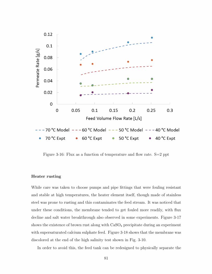
Figure 3-16: Flux as a function of temperature and flow rate. S=2 ppt
Heater rusting
While care was taken to choose pumps and pipe fittings that were fouling resistant
and stable at high temperatures, the heater element itself, though made of stainless
steel was prone to rusting and this contaminates the feed stream. It was noticed that
under these conditions, the membrane tended to get fouled more readily, with flux
decline and salt water breakthrough also observed in some experiments. Figure 3-17
shows the existence of brown rust along with CaSO4 precipitate during an experiment
with supersaturated calcium sulphate feed. Figure 3-18 shows that the membrane was
discolored at the end of the high salinity test shown in Fig. 3-10.
In order to avoid this, the feed tank can be redesigned to physically separate the
81

Figure 3-17: Rust seen on heater element in CaSO4 supersaturation experiments
heater element from the feed solution. For this purpose, a batch tank liner bag made
of polypropylene has been used. This bag is filled inside with pure water or tap water
which is heated by the heater. The flow around the bag induced by the outflow and
inflow of feed in the main tank enables good heat transfer from the large surface
area of the bag to the actual feed solution. A cylindrical wire structure is also used
for preventing direct contact of the bag with the heater which can cause the bag to
melt. Figure 3-19 illustrates this apparatus. This contraption was used successfully
to prevent fouling.
3.6 Conclusions
The design methodology and steps in the design of an air-gap membrane distillation
lab scale experimental setup were presented in detail. In particular the design features
essential for an experimental setup used to evaluate scaling and fouling in MD are
considered.
Some unique challenges that are encountered in this experimental procedure such
as changes in air gap width, difficulty in replacing membranes, heater scaling etc. are
discussed and innovative design solutions are presented where applicable.
82

Figure 3-18: Membrane used for experiment (Fig. 3-10) showing discoloration
The experimental setup was used to study the purification of sodium chloride
solutions at high concentrations. Some important results from this study include:
1. Permeate salinity maintained below 0.05 ppt (0.005%) after several days of
operation with highly saline 200 ppt (20%) sodium chloride feed solution. MD
is suitable for high salinity feed treatment
2. 20% reduction in flux with a 4.25x increase in salinity of feed stream. Initially,
flux declines linearly with salinity. Faster decline is observed beyond 100 ppt
due to deviation from ideal solution behavior
3. Raolts law combined with the film model of concentration polarization can
explain the flux decline observed for NaCl feed solutions. The maximum per-
centage difference between experimental measurements and numerical data is
10%, when the air gap thickness is maintained relatively constant. This con-
centration polarization model can be used as a baseline for further fouling tests
to find out further reductions in flux caused by membrane fouling.
4. Membrane orientation may affect the extent of polarization for asymmetric
membranes. This effect needs to be investigated further under high temper-
ature and salinity conditions where it becomes discernible.
5. The difficulty associated with experimentally varying feed flow rate as an in-
83

Figure 3-19: Heater separated from feed tank using a plastic bag
dependent parameter without affecting the more sensitive air gap thickness is
discussed.
84
Chapter 4
Effect of Module Inclination Angle
on Air Gap Membrane Distillation
Flux
David E. M. Warsinger contributed to this chapter.
Abstract
Air gap membrane distillation (AGMD) experiments were performed with varied tem-perature and varied module inclination angles to characterize the effect of moduleinclination angle on permeate production. While AGMD is potentially one of themost energy efficient membrane distillation configurations, transport resistances inthe air gap typically dominate, often dictating the flux performance of a system. Tilt-ing the module away from vertical offers the opportunity to manipulate the condensatelayer and its associated thermal resistance. In this chapter, we report experiments onvarying module tilt angle performed with a flat plate AGMD setup under fully char-acterized heat and mass transfer conditions. Numerical modeling is also performed tobetter understand the experimental results. The tests indicated that the AGMD systembehaves as a permeate gap, or flooded membrane distillation system for declined andextremely inclined positions. A key finding relevant to all AGMD systems is that athighly negative tilt angles (more than 30 degrees), condensate may fall onto the mem-brane causing thermal bridging and increased permeate production. Near vertical andpositive tilt angles (<15 degrees from vertical) show no significant effect of module tilton performance, in line with model predictions.
85

4.1 Introduction
Membrane distillation (MD) is an emerging thermally-powered desalination technol-
ogy with unique advantages at small scales, and potential to reach superior efficiencies
compared to existing desalination technologies. In an MD system, a hot, saline solu-
tion with a high vapor pressure flows across a hydrophobic membrane which selectively
allows water vapor to pass through but not liquid water or dissolved salts. Pure water
diffuses through the membrane and is condensed and collected on the other side. Due
to its scalability and low maintenance, most applications to date for this emerging
technology have been for small installations, some driven by solar thermal power [54].
Recent papers have suggested that MD can theoretically provide superior efficiencies
to all other thermal desalination technologies, including Multi-Stage Flash (MSF) and
Multi-Effect Distillation (MED) [55, 56], although actual test results have shown more
modest thermal performance [57]. Several configurations have been designed for MD,
including the most commonly, Direct Contact Membrane Distillation (DCMD) and
Air Gap Membrane Distillation (AGMD), as well as Vacuum Membrane Distillation
(VCMD), and Sweeping Gas Membrane Distillation (SGMD) [20]. Of these config-
urations, it has been shown that AGMD has higher potential for superior thermal
efficiencies [2].
AGMD includes a saline feed, a hydrophobic membrane, an air gap behind the
membrane, and a condensing surface beyond the air gap. Various configurations have
been designed, including flat sheet designs, a tubular configuration with concentric
cylinders, hollow fiber modules and spiral wound modules [20]. This study examines
the effect of varying the tilt angle of AGMD modules, which is primarily applicable
to flat plate configurations, but also to tubular and spiral wound systems. Flat plate
systems are among the most common due to their ease of manufacturing and assembly,
and are used in experimental systems as well as commercial modules such as those
produced by MEMSYS [58].
In AGMD systems with small air gaps, an important phenomenon that can occur
during operation is flooding and associated thermal bridging. Flooding occurs when
86

Figure 4-1: AGMD at varied angles
the permeate production rate exceeds the rate of condensate removal from the air gap.
This effect reduces mass transfer resistance, tending to increase permeate production
rate, but it also increases heat loss from and temperature polarization in the feed
channel as heat is conducted directly through the water from the membrane to the
cooling plate. Thermal bridging may also occur at small, localized regions at which
water falls from the condenser onto the membrane surface for declined tilt angles, if
local bridging of the membrane and condensation plate occurs. As this phenomenon
is unsteady and localized, it cannot be readily modeled in the generic model.
Module tilt angle has been studied in many condensation technologies. While
the vertical module orientation has been the norm in AGMD studies [59], horizontal
module orientation has also been used in some cases [60], which we define here as
angles approaching positive 90◦ from vertical as seen in Fig. 4-1. While relatively
unimportant in other configurations such as DCMD, where tilt angle only has hy-
drostatic effects, the module tilt angle affects droplet flow and film thickness on the
condenser surface in AGMD systems. The literature generally lacks experiments at
other angles, although 45 degrees has been examined for DCMD, not AGMD, config-
urations in experiments using bubbles to encourage turbulence [61]. To the authors’
87
knowledge, the present study is the first detailed experimental and theoretical analy-
sis of the effect and optimization of tilt angle on an AGMD process, and the first to
examine declined angles for AGMD.
4.2 Apparatus Design
The AGMD apparatus used is the one whose construction and design were discussed
in detail in Chapter 3. The module can be oriented at both positive and negative
angles from the vertical as shown in Fig. 4-1. The positive angles are more stable and
larger positive angles can be achieved (up to 90◦ possible), whereas on the negative
side, the maximum angle that was tested was −60◦.
To analyze the effect of module tilt angle, experiments were performed on the
AGMD test bed at various inclination angles under different combinations of feed
and cold side temperature conditions and with different air gap spacer meshes [62].
4.3 Numerical Modeling
4.3.1 Modeling Methods and Feed Channel Modeling
The theoretical performance of the AGMD system at varied angles is estimated using
numerical modeling techniques with Engineering Equation Solver (EES) [23], which is
an iterative equation solver with several thermodynamic property functions built into
it. A one-dimensional modeling approach is followed in which the temperatures and
flow rates vary along the length of the module. The width of the module is assumed
to be long so that the effect of the walls is negligible and properties are constant along
this direction. In the depth direction, the boundary layers and associated resistances
are taken into account, and the difference between the temperature and concentration
for the bulk stream and at the membrane interface is evaluated using suitable heat
and mass transfer coefficients.
The primary modeling calculations involve mass and energy conservation equa-
tions applied to each of the module sections: the feed channel, the air gap, and the
88

coolant channel (Figure 4-2). Each section is coupled with suitable transport equa-
tions. A detailed description of the overall modeling methodology applied for the
case of vertical module orientation is given by Summers et al. [2]. The heat and
mass transfer coefficients are determined through the Nusselt and Sherwood numbers
evaluated within each stream. The equations are solved using EES, and the number
of computational cells was progressively increased to 120, by which point the results
were seen to be grid independent.
Some important features of the model relevant to variations in flux associated
with module orientation are discussed below.
Figure 4-2: Computational cell of the AGMD model from [2].
The mass of water vapor transferred through the membrane is given by the mem-
brane characteristic equation (Eq. 4.1) and depends on the water vapor pressure on
either side of the membrane. The mass flow rate in the feed stream reduces corre-
spondingly.
J = B × (Pvap,f,m − Pvap,a,m) (4.1)
Here J is the permeate flux, B is the membrane permeability, Pvap,f,m is the vapor
pressure on the feed side surface of the membrane, and Pvap,a,m is the vapor pressure
on the air gap side surface of the membrane.
89
4.3.2 Air Gap and Condensing Channel Modeling
The air gap modeling is especially important since the transport resistances in this
region significantly affect the AGMD module performance. Varying the tilt angle
of the module can affect the process only through physical changes in this region.
Typically, a spacer mesh is placed in this region to prevent the flexible membrane
from collapsing onto the condensation surface. Like most other numerical models
of the AGMD module, the spacer is not explicitly considered and a free air gap is
modeled.
During operation, part of the membrane is pressed down into the gaps in the
mesh and the effective air gap depth is reduced. For modeling purposes though, the
membrane is considered to be flat for simplicity. No condensation or heat transfer
through the polypropylene mesh spacer is considered. The effective depth of the air
gap is taken at a value lower than the design value (1 mm) in order to account for
these effects. The water vapor flux entering the air gap diffuses through the air layer
to reach the film and condense. Since the air gap is thin, any convection effects are
ignored.
The flux through the membrane is a function of the vapor fraction at the interface
on the air gap side. The vapor diffuses to the water interface from this interface. The
diffusion is governed by binary mass diffusion as described in Lienhard and Lienhard
[30] as:
JmMw
=caDw−a
dgap − δln
(1 +
xi − xa,mxa,m − 1
)(4.2)
Here, Jm is the flux through the membrane, Mw is the molecular weight of water,
ca is the concentration of air, Dw−a is the diffusivity of water in air, dgap is the air
gap width, ξ is the water mole fraction at the liquid-vapor interface, and xa,m is the
water mole fraction at the membrane interface. The thickness of the air gap increases
as more liquid condenses into it. By mass conservation, assuming no shear at the
liquid-air interface, the rate of growth of the film can be evaluated as
90

δ3i+1 = δ3
i +3 Ji νf,i dA
g cosθ (ρf − ρg)w(4.3)
where δi is the condensation film thickness, dA is the differential of area, νf is the
fluid kinematic viscosity, g is the gravitational constant, ρf is the fluid density, ρg is
the combined air and water vapor density, and w is the width [63].
Note that the denominator here has cos (θ) to account for the angle of inclination.
When the module is vertical, θ = 0◦. The formula is used for angles as high as 85◦,
since the evaluated film thickness is still smaller than the air gap thickness. The heat
of condensation is conducted across the film, through the aluminum wall, and into
the coolant liquid.
4.3.3 Modeling Inputs
The numerical model takes the following inputs: geometry of the experimental setup
including the length, width, and depth of each of the channels; hot water flow rate
and temperature as it enters the module; and cold water flow rate and temperature
at module inlet.
4.3.4 Effect of Module Tilt Angle
Figure 4-3 shows the effect of tilt angle on flux in the model. The permeate production
rate at a given module inclination is normalized with respect to the flux at vertical
orientation and the ratio is plotted with respect to inclination angle. With all other
conditions remaining the same, the thickness of the condensate film is affected by
angle (Eq. 4.3). With a thicker film, the effective diffusion length (dgap− δ) for water
vapor is reduced, and hence the flux increases (Eq. 4.2). This effect is independent
of whether the module tilt angle is in the positive or negative direction.
An increase of around 4% is possible at very large module tilt angles as a result
of the film becoming thicker. Figure 4-3 shows that this increase is higher for cases
with lower cold side temperatures since viscosity of the film is higher and hence the
film rolls off the surface slower. This small increase does not include the effects of
91

thermal bridging or flooding.
Figure 4-3: Effect of module tilt angle on flux predicted by model
4.4 Methodology
4.4.1 Experimental Methodology
The measured permeate production rates, adjusted for temperature variability, are
presented. The hot side inlet and cold side inlet temperatures were set and maintained
using temperature controllers during experiment operation. The hot side temperature
in this experiment varies by ±0.2 ◦C over the course of an experiment; and on the
cold side, the temperature controller, which actuates a coolant flow valve, achieves
temperature control of ±0.5 ◦C around the set-point temperature. Between experi-
ments at different angles, the average inlet temperatures of the streams can change.
The difference in average temperature on the feed side is at most 0.4 ◦C and on the
92

cold side it is at most 1 ◦C. While Fig. 5 shows the relatively minute effect of tilt
angle on flux, the stream temperatures have a much larger influence on flux. This
is especially true because vapor pressure, which is the driving force for MD mass
transfer, is an exponential function of temperature. In order to separate the effect of
angle, the variability caused by small changes in average inlet temperatures must be
identified and removed.
Using the corresponding average inlet temperature and flow rate conditions at
each of the tilt angles, flux is estimated using the EES model for a vertical module
operating under those conditions. The measured flux for the AGMD experimental
system at vertical orientation was between 150-250 L/m2 day depending on the feed
flow conditions and the type and thickness of the air gap spacer used. The measured
permeate production rates are scaled by multiplying by vertical module flux obtained
from EES at the same temperature conditions divided by the experimentally obtained
flux at 0◦ tilt angle. The scaled experimental fluxes are then each divided by scaled
flux at 0◦. The ratio obtained is called the normalized permeate rate and will have
a value of unity at 0◦ tilt angle. At other tilt angles, the deviation from unity would
indicate the relative change in flux that results from tilting the apparatus if other
conditions were to remain exactly the same.
4.4.2 Uncertainty Quantification
Uncertainty analysis was performed within the EES code to account for uncertainties
in numerically predicted flux as a result of uncertainties in measured temperatures and
flow rates of the hot and cold streams. The overall uncertainty in flux was generally
dominated by temperature variations. While the hot side temperature has a larger
impact on flux, the absolute uncertainty in cold side temperature is higher, so that
both affect overall uncertainty. The uncertainty in actual temperature measurements
was estimated conservatively as the standard deviation in temperature recorded dur-
ing the experiment plus the maximum measurement uncertainty of ±0.2 ◦C for the
thermistors used.
Experimentally, the flux is determined over a period of 10-15 minutes by sub-
93
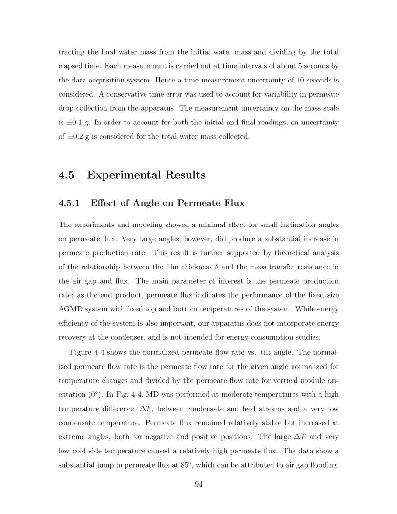
tracting the final water mass from the initial water mass and dividing by the total
elapsed time. Each measurement is carried out at time intervals of about 5 seconds by
the data acquisition system. Hence a time measurement uncertainty of 10 seconds is
considered. A conservative time error was used to account for variability in permeate
drop collection from the apparatus. The measurement uncertainty on the mass scale
is ±0.1 g. In order to account for both the initial and final readings, an uncertainty
of ±0.2 g is considered for the total water mass collected.
4.5 Experimental Results
4.5.1 Effect of Angle on Permeate Flux
The experiments and modeling showed a minimal effect for small inclination angles
on permeate flux. Very large angles, however, did produce a substantial increase in
permeate production rate. This result is further supported by theoretical analysis
of the relationship between the film thickness δ and the mass transfer resistance in
the air gap and flux. The main parameter of interest is the permeate production
rate; as the end product, permeate flux indicates the performance of the fixed size
AGMD system with fixed top and bottom temperatures of the system. While energy
efficiency of the system is also important, our apparatus does not incorporate energy
recovery at the condenser, and is not intended for energy consumption studies.
Figure 4-4 shows the normalized permeate flow rate vs. tilt angle. The normal-
ized permeate flow rate is the permeate flow rate for the given angle normalized for
temperature changes and divided by the permeate flow rate for vertical module ori-
entation (0◦). In Fig. 4-4, MD was performed at moderate temperatures with a high
temperature difference, ∆T , between condensate and feed streams and a very low
condensate temperature. Permeate flux remained relatively stable but increased at
extreme angles, both for negative and positive positions. The large ∆T and very
low cold side temperature caused a relatively high permeate flux. The data show a
substantial jump in permeate flux at 85◦, which can be attributed to air gap flooding.
94

Figure 4-4: Effect of module tilt angle on permeate production: Tf,in = 50 ◦C, Tc,in =12.5 ◦C
For this nearly horizontal case, the role of gravity in draining the film is substantially
diminished (cf. Eq. 3). Additionally, for the low condenser temperature of 12.5 ◦C,
the viscosity of liquid water is roughly twice the value in later trials at 30 ◦C, also
contributing somewhat to a thicker condensate film.
Figure 4-5, for a trial at significantly higher temperature than Fig. 4-4, shows that
angle played a small role in positive and moderately negative angles, but that flux
increased significantly at very large negative angles. This may be indicative of thermal
bridging at relatively small negative angles such as −30◦, rather than flooding, and
a tendency to flood as the module tilt angle further increases and approaches −60◦.
Since it is almost universally observed that thermal bridging or other effects of
module tilt angle variation are effectively absent at low tilt angles, subsequent trials
reduced the number of angles considered in the low angle range.
To further investigate the hypotheses of thermal bridging and flooding, additional
95
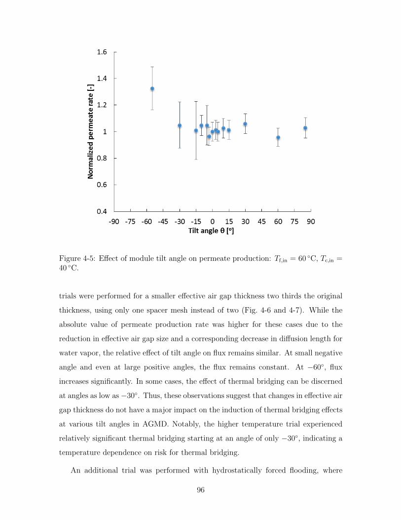
Figure 4-5: Effect of module tilt angle on permeate production: Tf,in = 60 ◦C, Tc,in =40 ◦C.
trials were performed for a smaller effective air gap thickness two thirds the original
thickness, using only one spacer mesh instead of two (Fig. 4-6 and 4-7). While the
absolute value of permeate production rate was higher for these cases due to the
reduction in effective air gap size and a corresponding decrease in diffusion length for
water vapor, the relative effect of tilt angle on flux remains similar. At small negative
angle and even at large positive angles, the flux remains constant. At −60◦, flux
increases significantly. In some cases, the effect of thermal bridging can be discerned
at angles as low as −30◦. Thus, these observations suggest that changes in effective air
gap thickness do not have a major impact on the induction of thermal bridging effects
at various tilt angles in AGMD. Notably, the higher temperature trial experienced
relatively significant thermal bridging starting at an angle of only −30◦, indicating a
temperature dependence on risk for thermal bridging.
An additional trial was performed with hydrostatically forced flooding, where
96
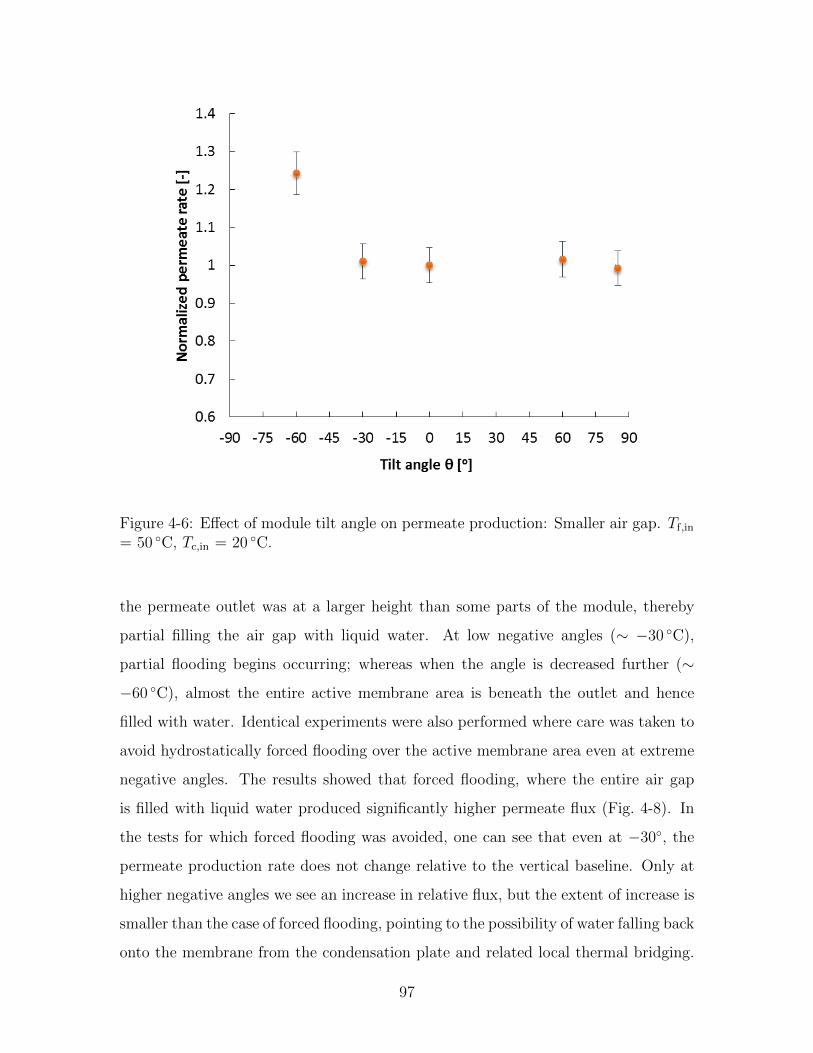
Figure 4-6: Effect of module tilt angle on permeate production: Smaller air gap. Tf,in
= 50 ◦C, Tc,in = 20 ◦C.
the permeate outlet was at a larger height than some parts of the module, thereby
partial filling the air gap with liquid water. At low negative angles (∼ −30 ◦C),
partial flooding begins occurring; whereas when the angle is decreased further (∼
−60 ◦C), almost the entire active membrane area is beneath the outlet and hence
filled with water. Identical experiments were also performed where care was taken to
avoid hydrostatically forced flooding over the active membrane area even at extreme
negative angles. The results showed that forced flooding, where the entire air gap
is filled with liquid water produced significantly higher permeate flux (Fig. 4-8). In
the tests for which forced flooding was avoided, one can see that even at −30◦, the
permeate production rate does not change relative to the vertical baseline. Only at
higher negative angles we see an increase in relative flux, but the extent of increase is
smaller than the case of forced flooding, pointing to the possibility of water falling back
onto the membrane from the condensation plate and related local thermal bridging.
97
Figure 4-7: Effect of module tilt angle on permeate production: Smaller air gap. Tf,in
= 60 ◦C, Tc,in = 40 ◦C.
This further demonstrates that both flooding and thermal bridging are possibilities
in AGMD at high inclinations and that the relative increase in flux is affected greatly
by the extent of thermal bridging.
4.5.2 Thermal Bridging Hypothesis
The thermal bridging may occur if fluid falls from the condensing plate onto the
membrane itself, forming a liquid bridge across the local air gap. This phenomenon is
not captured by the numerical model. Thermal bridging is particularly likely in the
case of negative tilt angles and hence the experimental flux results are asymmetric
about the 0◦ orientation. As the mass transfer resistance is dominated by the air
gap width, this phenomena should be easily observed by an increase in permeate
flux at declined angles. Our initial hypothesis was that bridging could occur even at
small negative angles. In the experimental data, however, we see no such change in
98

Figure 4-8: Effect of module tilt angle on permeate production: Comparison withmodified experiment where hydrostatic forced flooding is avoided. Tf,in = 50 ◦C, Tc,in
= 20 ◦C
permeate flux at small negative angles, indicating a lack of thermal bridging. The key
insight is that thermal bridging is not a concern at vertical and near vertical angles
for the air gap and spacer dimensions considered here.
An explanation for the why fluid does not fall onto the MD membrane even at
negative inclinations may be obtained by the considering the hydrophobicity or hy-
drophilicity of the surface on which the fluid flows. The aluminum condensing surface
is hydrophilic: typical aluminum condensing surfaces have contact angles around 5◦
[64]. Meanwhile, MD membranes are hydrophobic. Thin films of water can remain
on the underside of inclined hydrophilic surfaces up to very high angles of inclination
[65, 66, 67]. Additionally, in small gaps where droplets can easily exceed the size of
the gap, droplets on the hydrophobic surface may touch and be reabsorbed into the
film on the hydrophilic condensing plate. Therefore, large tilt angles, which favor
thicker liquid films, may be required before thermal bridging effects occur.
99
4.6 Conclusions
The experimental and theoretical results indicate that moderate angles of inclination
only had a minor effect on permeate flux, except at high angles where it was quite
significant. Permeate flux varied by less than 5% within inclination angles of ±15◦,
but flux increased significantly as angles approached ±90◦, in some cases rising by
more than 40%.
The results indicate AGMDs susceptibility to two conditions in which liquid water
spans the air gap, flooding and thermal bridging. Flooding, occurring when permeate
production was rapid enough to fill the air gap with permeate, is a risk at large
temperature differences across the air gap, at small gap sizes, and at very high inclined
or declined angles. Flooding occurs primarily at very high inclined or declined angles.
The second condition, thermal bridging, occurs at high declined angles, for which
condensate detaches from the laminar film on the condenser plate and makes contact
with the hot membrane surface. This condition occurred more readily than flooding
at declined angles, but was not observed for angles less than 30◦ off vertical. Results
suggest that thermal bridging and flooding are likely to occur earlier, at smaller
negative inclination angles, in systems that have lower air gap thickness.
While in many cases flooding and thermal bridging may reduce thermal efficiency,
in single pass systems with limited size or lacking energy recovery, the increased
permeate production from high incline angles with flooding or thermal bridging is
often desirable, as more pure water is produced under the same cycle top and bottom
temperature conditions.
100

Bibliography
[1] M. El-Bourawi, Z. Ding, R. Ma, and M. Khayet, “A framework for better un-derstanding membrane distillation separation process,” Journal of MembraneScience, vol. 285, pp. 4–29, Nov. 2006.
[2] E. K. Summers, H. A. Arafat, and J. H. Lienhard, “Energy efficiency compar-ison of single-stage membrane distillation (MD) desalination cycles in differentconfigurations,” Desalination, vol. 290, pp. 54–66, 2012.
[3] U. N. D. Program, “Human development report.” http://www.un.org/
waterforlifedecade/scarcity.shtml,2006.
[4] IDA, “Desalination yearbook, section 1. market profile.” International Desalina-tion Association, 2011 - 2012.
[5] K. H. Mistry, R. K. McGovern, G. P. Thiel, E. K. Summers, S. M. Zubair, andJ. H. Lienhard V, “Entropy Generation Analysis of Desalination Technologies,”Entropy, vol. 13, pp. 1829–1864, Sept. 2011.
[6] K. B. Gregory, R. D. Vidic, and D. A. Dzombak, “Water management challengesassociated with the production of shale gas by hydraulic fracturing,” Elements,vol. 7, no. 3, pp. 181–186, 2011.
[7] E. Curcio and E. Drioli, “Separation & Purification Reviews Membrane Distilla-tion and Related Operations – A Review,” Separation and Purification Reviews,vol. 34, pp. 35–86, 2005.
[8] A. S. Hassan and H. E. Fath, “Review and assessment of the newly developed MDfor desalination processes,” Desalination and Water Treatment, vol. 51, no. 1-3,pp. 574–585, 2013.
[9] S. Shirazi, C.-J. Lin, and D. Chen, “Inorganic fouling of pressure-driven mem-brane processes – A critical review,” Desalination, vol. 250, no. 1, pp. 236–248,2010.
[10] H. Susanto, “Towards practical implementations of membrane distillation,”Chemical Engineering and Processing: Process Intensification, vol. 50, no. 2,pp. 139–150, 2011.
101

[11] M. Khayet, “Membranes and theoretical modeling of membrane distillation: areview,” Advances in colloid and interface science, vol. 164, no. 1-2, pp. 56–88,2011.
[12] Edited by Belmiloudi, Aziz, Heat Transfer - Theoretical Analysis, ExperimentalInvestigations and Industrial Systems. InTech, 2011.
[13] K. Lawson and D. Lloyd, “Membrane distillation,” Journal of Membrane Science,vol. 124, no. 1, pp. 1–25, 1997.
[14] A. Antony, J. H. Low, S. Gray, A. E. Childress, P. Le-Clech, and G. Leslie, “Scaleformation and control in high pressure membrane water treatment systems: Areview,” Journal of Membrane Science, vol. 383, no. 1-2, pp. 1–16, 2011.
[15] R. B. Saffarini, E. K. Summers, H. A. Arafat, and J. H. Lienhard V, “Eco-nomic evaluation of stand-alone solar powered membrane distillation systems,”Desalination, vol. 299, pp. 55–62, 2012.
[16] J. Koschikowski, M. Wieghaus, and M. Rommel, “Solar thermal-driven desali-nation plants based on membrane distillation,” Desalination, vol. 156, no. 1-3,pp. 295–304, 2003.
[17] F. Banat, N. Jwaied, M. Rommel, J. Koschikowski, and M. Wieghaus, “Desalina-tion by a “compact SMADES” autonomous solar powered membrane distillationunit,” Desalination, vol. 217, no. 1-3, pp. 29–37, 2007.
[18] F. Banat, N. Jwaied, M. Rommel, J. Koschikowski, and M. Wieghaus, “Perfor-mance evaluation of the “large SMADES” autonomous desalination solar-drivenmembrane distillation plant in Aqaba, Jordan,” Desalination, vol. 217, no. 1-3,pp. 17–28, 2007.
[19] E. Guillen-Burrieza, R. Thomas, B. Mansoor, D. Johnson, N. Hilal, andH. Arafat, “Effect of dry-out on the fouling of PVDF and PTFE mem-branes under conditions simulating intermittent seawater membrane distillation(SWMD),” Journal of Membrane Science, vol. 438, pp. 126–139, 2013.
[20] A. Alkhudhiri, N. Darwish, and N. Hilal, “Membrane distillation: A comprehen-sive review,” Desalination, vol. 287, pp. 2–18, Feb. 2012.
[21] L. Martinez-Diez and M. Vazquez-Gonzalez, “Temperature and concentrationpolarization in membrane distillation of aqueous salt solutions,” Journal of Mem-brane Science, vol. 156, no. 2, pp. 265 – 273, 1999.
[22] G. P. Narayan, M. H. Sharqawy, S. Lam, S. K. Das, and J. H. Lienhard V,“Bubble columns for condensation at high concentrations of non condensablegas: Heat transfer model and experiments,” AIChE Journal, vol. 59, no. 5,pp. 1780–1790, 2012.
102

[23] S.A.Klein, “Engineering equation solver version 9.” http://www.fchart.com/
ees/.
[24] R. Hyland and A. Wexler, “Formulations for the thermodynamic properties ofthe saturated phases of H2O from 173.15K to 473.15K,” ASHRAE Transactions(Part 2A), 1983.
[25] A. Pruss and W. Wagner, “The IAPWS formulation 1995 for the thermodynamicproperties of ordinary water substance for general and scientific use,” Journal ofPhysical and Chemical Reference Data, vol. 2, pp. 387–535, 2002.
[26] M. Khayet, P. Godino, and J. I. Mengual, “Theory and experiments on sweepinggas membrane distillation,” Journal of Membrane Science, vol. 165, no. July1999, pp. 261–272, 2000.
[27] M. Khayet, M. P. Godino, and J. I. Mengual, “Thermal boundary layers in sweep-ing gas membrane distillation processes,” AIChE Journal, vol. 48, pp. 1488–1497,July 2002.
[28] K. Charfi, M. Khayet, and M. Safi, “Numerical simulation and experimentalstudies on heat and mass transfer using sweeping gas membrane distillation,”Desalination, vol. 259, pp. 84–96, Sept. 2010.
[29] J. Swaminathan and J. H. Lienhard V, “Energy efficiency of Sweeping Gas Mem-brane Distillation cycles,” in Proceedings of the 11th ISHMT-ASME Heat andMass Transfer Conf., Kharagpur, ISHMT-ASME, 2013.
[30] J. H. Lienhard V and J. H. Lienhard IV, A Heat Transfer Textbook, FourthEdition. Dover Publications, Inc., 2011.
[31] E. W. Tow and J. H. Lienhard V, “Heat Flux and Effectiveness in Bubble ColumnDehumidifiers,” in Proceedings of the 2013 IDA World Congress on Desalinationand Water Reuse, IDA, 2013.
[32] G. P. Narayan, J. H. Lienhard V, and S. M. Zubair, “Entropy generation mini-mization of combined heat and mass transfer devices,” International Journal ofThermal Sciences, vol. 49, no. 10, pp. 2057 – 2066, 2010.
[33] C. Cabassud and D. Wirth, “Membrane distillation for water desalination: Howto choose an appropriate membrane?,” Desalination, vol. 157, no. 1-3, pp. 307–314, 2003.
[34] D. L. Shaffer, L. H. Arias Chavez, M. Ben-Sasson, S. Romero-Vargas Castrillon,N. Y. Yip, and M. Elimelech, “Desalination and reuse of high-salinity shale gasproduced water: drivers, technologies, and future directions,” Environmentalscience & technology, vol. 47, no. 17, pp. 9569–9583, 2013.
[35] M. Khayet and T. Matsuura, Membrane Distillation Principles and Applications.Elsevier, 2011.
103

[36] N. Epstein, “Thinking about heat transfer fouling: A 5 5 matrix,” Heat TransferEngineering, vol. 4, no. 1, pp. 43–56, 1983.
[37] T. Y. Cath, V. Adams, and A. E. Childress, “Experimental study of desalinationusing direct contact membrane distillation: a new approach to flux enhance-ment,” Journal of Membrane Science, vol. 228, no. 1, pp. 5 – 16, 2004.
[38] E. K. Summers, Energy Efficiency of membrane distillation. PhD thesis, Mas-sachusetts Institute of Technology, 2013.
[39] McMaster-Carr, “Viton Fluoroelastomer O-Ring Cord Stock , Part Number96515K42.” http://www.mcmaster.com/?error_redirect=true#96515k42/
=rrt8jz.
[40] R. D. Blevins, Applied Fluid Dynamics Handbook. Krieger Publishing, 2003.
[41] Millipore, “Immobilon-PSQ Membrane, PVDF, Part Number ISEQ00010.”http://www.millipore.com/catalogue/item/ISEQ00010.
[42] Cole-Parmer, “Magnetic Drive PP Centrifugal Pump with EnclosedMotor; 18.4 GPM/26.9 ft, 115V, Part Number 72010-60.” http:
//www.coleparmer.com/Product/Mag_Drive_PP_Centrifugal_Pump_w_
Enclosed_Motor_18_4_GPM_26_9_ft_115V/EW-72010-60.
[43] Cole-Parmer, “Magnetic Drive PP Centrifugal Pump with EnclosedMotor; 8.2 GPM/14.1 ft, 115V, Part Number 72010-30.” http:
//www.coleparmer.com/Product/Mag_Drive_PP_Centrifugal_Pump_w_
Enclosed_Motor_8_2_GPM_14_1_ft_115V/EW-72010-30.
[44] Omega, “Pipe-Plug Thermistor Probes, Part Number TH-44004-1/4NPT-80.”http://www.omega.com/pptst/TH-44000-NPT.html.
[45] Cole-Parmer, “Cole-Parmer multi-sensor temperature logger w/onboard memorycard, Part Number USB-5203.” http://www.coleparmer.com/buy/product/
68114-cole-parmer-multi-sensor-temperature-logger-w-onboard-memory-card.
html.
[46] McMaster-Carr, “Splash-Resistant Water Flowmeter, 1/2 Pipe, Part Number3562K12.” http://www.mcmaster.com/#3562k12/=rrshfc.
[47] McMaster-Carr, “Splash-Resistant Water Flowmeter, 3/8 Pipe, Part Number3562K11.” http://www.mcmaster.com/#3562k11/=rrsi3p.
[48] McMaster-Carr, “Digital Bench Scale with Stainless Steel Platform 70.55oz/ 2000 G Capacity, Part Number 1760T86.” http://www.mcmaster.com/
#1760t86/=rrt04f.
[49] K. Scientific, “Jenco 3250 portable Conductivity meter.” http://www.katsci.
com/products/jenco-3250-portable-meter.aspx.
104

[50] A. L. Zydney, “Stagnant film model for concentration polarization in membranesystems,” Journal of Membrane Science, vol. 130, no. 1, pp. 275–281, 1997.
[51] S. Bhattacharjee, J. C. Chen, and M. Elimelech, “Coupled model of concentra-tion polarization and pore transport in crossflow nanofiltration,” AIChE journal,vol. 47, no. 12, pp. 2733–2745, 2001.
[52] K. H. Mistry and J. H. Lienhard, “Effect of nonideal solution behavior on de-salination of a sodium chloride (NaCl) solution and comparison to seawater,”in ASME 2012 International Mechanical Engineering Congress and Exposition,pp. 1509–1523, American Society of Mechanical Engineers, 2012.
[53] R. A. Robinson and R. H. Stokes, Electrolyte solutions. Courier Dover Publica-tions, 2002.
[54] E. K. Summers and J. H. Lienhard V, “A novel solar-driven air gap membranedistillation system,” Desalination and Water Treatment, vol. 51, pp. 1–8, 2012.
[55] J. Gilron, L. Song, and K. K. Sirkar, “Design for Cascade of Crossflow DirectContact Membrane Distillation,” Industrial & Engineering Chemistry Research,vol. 46, no. 8, pp. 2324–2334, 2007.
[56] F. He, J. Gilron, and K. K. Sirkar, “High water recovery in direct contact mem-brane distillation using a series of cascades,” Desalination, vol. 323, pp. 48–54,2013.
[57] G. Zaragoza, A. Ruiz-Aguirre, E. Guillen-Burrieze, D. Alarcon-Padilla, andJ. Blanco-Galvez, “Experimental comparison of different prototypes of solar en-ergy driven membrane distillation systems,” in Proceedings of the 2013 IDAWorld Congress on Desalination and Water Reuse, 2013.
[58] K. Zhao, W. Heinzl, M. Wenzel, S. Buttner, F. Bollen, G. Lange, S. Heinzl, andN. Sarda, “Experimental study of the memsys vacuum-multi-effect-membrane-distillation (V-MEMD) module,” Desalination, vol. 323, pp. 150–160, 2013.
[59] G. L. Liu, C. Zhu, C. S. Cheung, and C. W. Leung, “Theoretical and experimen-tal studies on air gap membrane distillation,” Heat and Mass Transfer, vol. 34,no. 4, pp. 329–335, 1998.
[60] A. Alkhudhiri, N. Darwish, and N. Hilal, “Produced water treatment: Applica-tion of air gap membrane distillation,” Desalination, pp. 46–51, 2013.
[61] G. Chen, X. Yang, R. Wang, and A. G. Fane, “Performance enhancement andscaling control with gas bubbling in direct contact membrane distillation,” De-salination, vol. 308, pp. 47–55, 2013.
[62] D. E. M. Warsinger, J. Swaminathan, and J. H. Lienhard V, “Effect of moduleinclination angle on Air Gap Membrane Distillation,” in Proceedings of the 15thInternational Heat Transfer Conference, IHTC, 2014.
105

[63] A. Mills, Heat Transfer 2nd Edition. Prentice Hall, 1998.
[64] J. Bernardin, I. Mudawar, C. Walsh, and E. Franses, “Contact angle temperaturedependence for water droplets on practical aluminum surfaces,” InternationalJournal of Heat and Mass Transfer, vol. 40, no. 5, pp. 1017–1033, 1997.
[65] H. R. Nagendra, “Effect of inclination on laminar film condensation,” AppliedScientific Research, vol. 28, pp. 261–277, 1973.
[66] J. A. Howarth, G. Poots, and D. Wynne, “Laminar film condensation on theunderside of an inclined flat plate,” Mechanics Research Communications, vol. 5,no. 6, pp. 369–374, 1978.
[67] B. J. Chung and S. Kim, “Film condensations on horizontal and slightly in-clined upward and downward facing plates,” Heat Transfer Engineering, vol. 29,pp. 936–941, 2008.
106