EXPERIMENTAL AND NUMERICAL SIMULATION OF FLOW OVER … · EXPERIMENTAL AND NUMERICAL SIMULATION OF FLOW OVER BROAD CRESTED WEIR AND STEPPED WEIR USING DIFFERENT TURBULENCE MODELS

Journal of Engineering and Sustainable Development Vol. 21, No. 02, March 2017 www.jeasd.org (ISSN 2520-0917)

28

;

EXPERIMENTAL AND NUMERICAL SIMULATION OF FLOW

OVER BROAD CRESTED WEIR AND STEPPED WEIR USING

DIFFERENT TURBULENCE MODELS

Dr. Shaymaa A. M. Al-Hashimi1, Dr. Huda M. Madhloom2, Thameen Nazar Nahi3*

1) Assist Prof. , Civil Engineering Department, Al-Mustansiriayah University, Baghdad, Iraq.

2) Lecture, Civil Engineering Department, Al-Mustansiriayah University, Baghdad, Iraq.

3) M.Sc. Student, Civil Engineering Department, Al-Mustansiriayah University, Baghdad, Iraq.

Abstract: A broad-crested weir has been considered the most hydraulic structures which was used in

open channels for flow measurement and to control the water surface levels due to its simplicity. Both experimental and numerical models were conducted on a broad crested weir and stepped weir with a

rounded corner. In this study, FLUENT software as a type of Computational Fluid Dynamics (CFD)

model, represented as a numerical model in order to simulate flow over weirs that govern by Reynold

averaged Navier Stoke equation and their results were compared with experimental results. The structured

mesh with high concentration near the wall regions was employed in the numerical model. The volume of

fluid (VOF) method with four turbulence models of Standard k–ε, RNG k–ε, Realizable k–ε and Standard

k–ω are applied to estimate the free surface profile. The result showed that the flow over weirs is

turbulent and the characteristics of free surface were complex and often difficult to be predicted. Also, the

comparison of water surface profile between experimental value and numerical results obtained from the

turbulent models showed that the standard k–ε model has the best similarity and standard k–ω model has

the minimum similarity with experimental value.

Keywords: Broad Crested Weir, Stepped Weir, Numerical CFD Model, FLUENT, VOF, Turbulent

Models.

ف انرحكى اندشا نقاس انفرحح قاخان ف اسرخذيد انر انذسنكح انشاءاخ انقح ي اكثش انسذ اسغ ؼرثش:الخالصة

ز ف. دائشح تزاح انسذ اسغ انقح انسذ انذسج ػهى أخشدكال انارج انؼذدح انردشثح . نثساطر ظشا انسطحح انا يسراخ

يحاكاج أخم ي ػذدي كرجComputational Fluid Dynamics (CFD ) ي كع FLUENTتشايح اسرخذاو ذى انذساسح،

ذى اسرخذاو . انردشثح انرائح يغ انرائح قسد Reynold averaged Navier Stoke انر ذحكى ي قثم يؼادنح انسذد ػثش انرذفق

انقاس االضطشابي ارج أستؼح( VOF) انائغ حدىطشقح .انؼذدي رجان ف اندذاس يطقح قشب ػال ذشكز كم انشثكح ر

k–ε ، RNG k–ε ، Realizable k–ε k–ω يضطشب انسذد ػهى انرذفقا انرائح، أظشخ .انسطح انحشنرخ شكم انقاسح

تم التي القيم العدديةو تجريبيةال قيمال بين السطحية المياه شكل مقارنة تم أيضا،. التنبؤ به صؼة يا غانثا يؼقذ انحش سطحان خصائص .تجريبية القيم مع كان اقل تشابه k–ω ونموذج أفضل تشابه قد القياسي k–ε بينت بانه نموذج ،االضطراب نماذج من عليها الحصول

1. Introduction

Weirs are building for passing water flow in critical conditions or for regulating the

water surface level. The most common types of weir crest in the practice are broad

*Corresponding Author [email protected]

Vol. 21, No. 02, March 2017 ISSN 2520-0917

www.jeasd.org

mailto:[email protected]


29

crested weir, sharp crested weir and ogee crest weir. These structures which built for

measuring the flow in open channels.

The broad crested weir was definition as a flat-crested structure with a length 'L' of

crest large enough compared to the flow thickness over crest. The crest is termed broad

when the flow streamlines are parallel to the crest and that critical depth is occurred

along the crest and the pressure distribution is hydrostatic [1]. Furthermore, the broad

crested weir gives it some outstanding characteristics over other forms of weir such as

stable overflow pattern, passing of floating debris easily, lower cost of construction and

easily designed when compared to other weirs.

In order to prevent erosion and scouring in downstream (D/S) ends of weirs, the

hydraulic energy should be dissipated [2], so that the flow characteristics over broad

crested weirs were investigated by several investigators with single step of broad crested

weir, that’s weir called stepped weir.

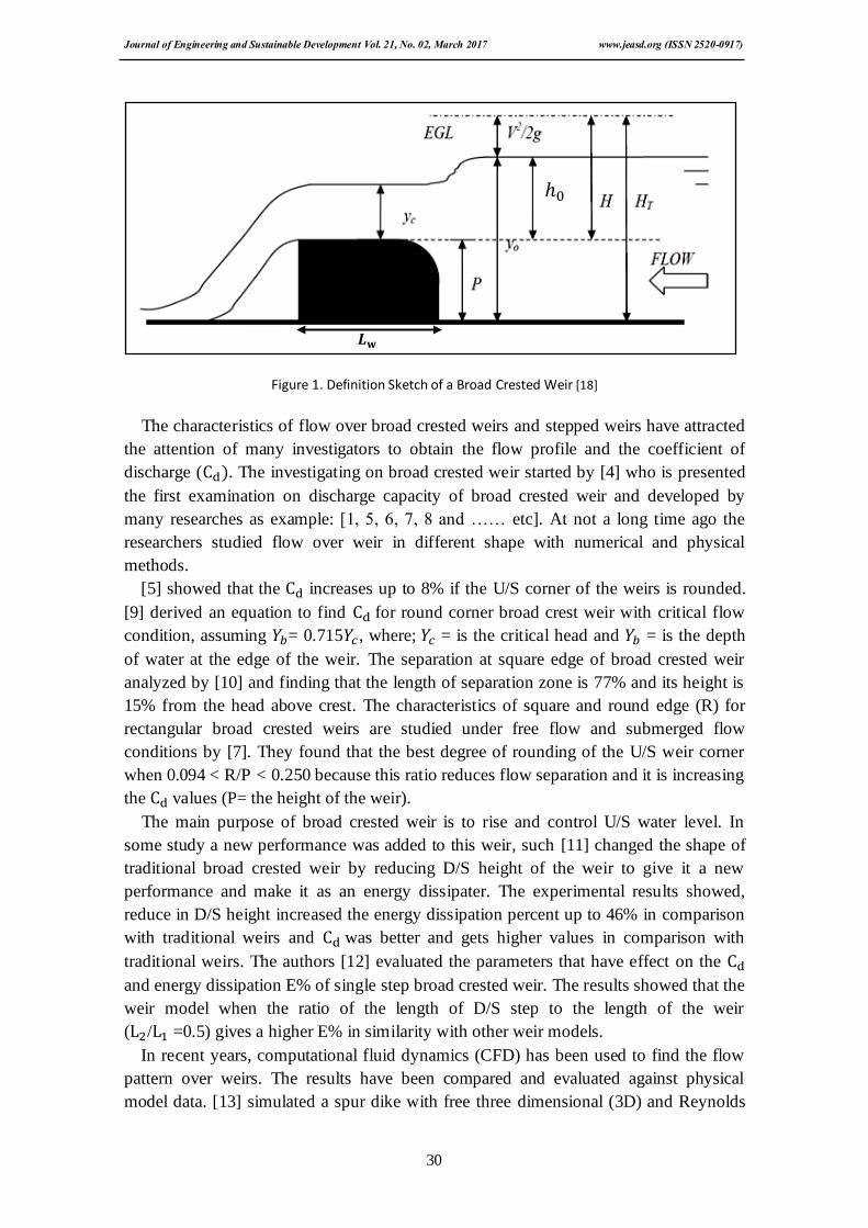
Based on Bernoulli equation, the flow equation of the weir, which shown in Fig. (1)

below, could express the following relationship in Equation (1) between weir discharge

and the head over the crest [3];

=

√

( ⁄ . B (1)

In real fluid, the head above crest of the weir is given by Equation (2);

= +

(2)

The approach velocity ⁄ ) is very small, so that equal to H in Eq.(1). Eq. (2)

becomes as Equation (3);

=

√

(

⁄ . B (3)

Where;

= is the actual discharge ( ⁄

= is the dimensionless coefficient of discharge

= is the gravitational acceleration ⁄

H = the head above weir crest with approach velocity (m)

= the head above weir crest without approach velocity (m)

B = width of the weir (the perpendicular direction to the flow) (m)


30

Figure 1. Definition Sketch of a Broad Crested Weir [18]

The characteristics of flow over broad crested weirs and stepped weirs have attracted

the attention of many investigators to obtain the flow profile and the coefficient of

discharge ( . The investigating on broad crested weir started by [4] who is presented

the first examination on discharge capacity of broad crested weir and developed by

many researches as example: [1, 5, 6, 7, 8 and …… etc]. At not a long time ago the

researchers studied flow over weir in different shape with numerical and physical

methods.

[5] showed that the increases up to 8% if the U/S corner of the weirs is rounded.

[9] derived an equation to find for round corner broad crest weir with critical flow

condition, assuming = 0.715 , where; = is the critical head and = is the depth

of water at the edge of the weir. The separation at square edge of broad crested weir

analyzed by [10] and finding that the length of separation zone is 77% and its height is

15% from the head above crest. The characteristics of square and round edge (R) for

rectangular broad crested weirs are studied under free flow and submerged flow

conditions by [7]. They found that the best degree of rounding of the U/S weir corner

when 0.094 < R/P < 0.250 because this ratio reduces flow separation and it is increasing

the values (P= the height of the weir).

The main purpose of broad crested weir is to rise and control U/S water level. In

some study a new performance was added to this weir, such [11] changed the shape of

traditional broad crested weir by reducing D/S height of the weir to give it a new

performance and make it as an energy dissipater. The experimental results showed,

reduce in D/S height increased the energy dissipation percent up to 46% in comparison

with traditional weirs and was better and gets higher values in comparison with

traditional weirs. The authors [12] evaluated the parameters that have effect on the

and energy dissipation E% of single step broad crested weir. The results showed that the

weir model when the ratio of the length of D/S step to the length of the weir

( / =0.5) gives a higher E% in similarity with other weir models.

In recent years, computational fluid dynamics (CFD) has been used to find the flow

pattern over weirs. The results have been compared and evaluated against physical

model data. [13] simulated a spur dike with free three dimensional (3D) and Reynolds


31

averaged Naveor Stokes (RANS) equations. The volume of fluid (VOF) and standard k-

ε method were used to simulate free surface and turbulence flow. [14] compared the

position of the free surface profile over a laboratory rectangular broad crested weir with

numerical CFD model. For the smaller flow rate they measured, the results showed that

the prediction of the U/S water depth was excellent and the rapidly varied flow profile

over the crest and a stationary wave profile was observed at D/S, where the flow was

supercritical.

The velocity and pressure measurements were studied numerically by [8] on broad

crested weir. Pressure and velocity distributions measurements were conducted

systematically and they showed the rapid redistributions of both velocity and pressure

fields at the U/S end of the weir crest. [15] describes the validation of CFD for free

surface flows over broad crested weir by using a published experimental dataset of [21]

and discusses the accuracy of CFD in being able to predict the free surface profile. The

study of [16] on a broad crested weir with a rounded corner is presented to investigate

the free surface profile of water by using the volume of fluid (VOF). The computational

results showed a good agreement with experimental result obtained in the laboratory.

[17] employed CFD model on triangular broad crested weir to investigate the flow

pattern over it. VOF with the RNG k -ε, standard k -ε and the large eddy simulation

(LES) were applied to find the water level profile and showed the RNG k -ε model has

the maximum accuracy with experimental data in comparison with other turbulence

models used. In the study of [18], laboratory model with CFD model was carried out on

broad crested weir located on rectangular channel to predict the value. Good

agreements between the laboratory value and the CFD value were obtained. The mean

relative error percentage (RE), root mean square errors (RMSE) and mean absolute

errors (MAE) for the are 3.043, 0.123 and 0.0987 respectively. The effect of

inclination from 90º to 23º weir in the U/S face of rectangular broad crested weirs and

flow characteristic is studied by [19] by using CFD model together with laboratory

model were applied to improve the performance of broad crested weirs in order to

reduce the effect of flow separation. Also the results showed, by decreasing the slope of

the U/S side, the discharge efficiency increased with slope of 23º about 22% higher than

the standard weir.

The objective of this study are to examine the laboratory measurements and 2D

numerical modeling which employed to simulate the flow pattern over a rectangular

broad crested weir and stepped weir located in a rectangular channel and comparison

between free surface profiles obtained from experiment and numerical results for

different turbulent models.

2. Experimental Work

The experiments tests were carried out in the Hydraulic Engineering Laboratory,

Department of Environmental Engineering, Collage of Engineering, Al-Mustansiriayah

University in Baghdad. In this research, the flume that was made of glass with a cross

section of 0.3 m wide, 0.3 m deep and 4.8 m long was shown in photo (A) and photo

(B). The broad crested weir was 0.15 m of height (P), 0.3 m of width (B) and as 0.36 m


32

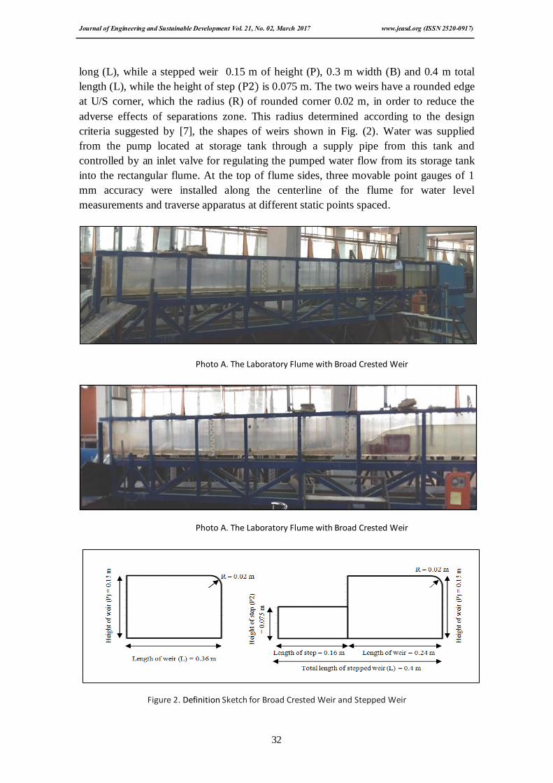
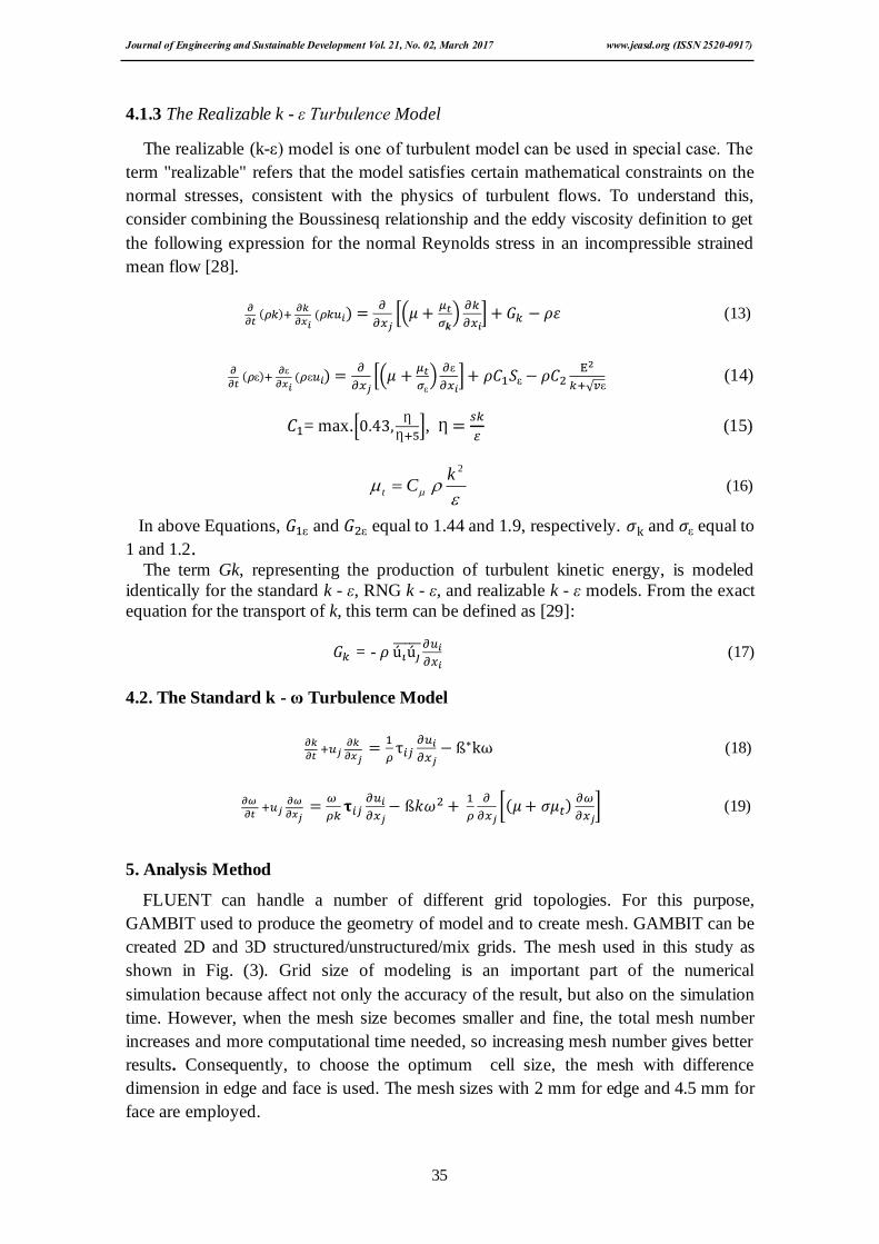
long (L), while a stepped weir 0.15 m of height (P), 0.3 m width (B) and 0.4 m total

length (L), while the height of step ( is 0.075 m. The two weirs have a rounded edge

at U/S corner, which the radius (R) of rounded corner 0.02 m, in order to reduce the

adverse effects of separations zone. This radius determined according to the design

criteria suggested by [7], the shapes of weirs shown in Fig. (2). Water was supplied

from the pump located at storage tank through a supply pipe from this tank and

controlled by an inlet valve for regulating the pumped water flow from its storage tank

into the rectangular flume. At the top of flume sides, three movable point gauges of 1

mm accuracy were installed along the centerline of the flume for water level

measurements and traverse apparatus at different static points spaced.

Photo A. The Laboratory Flume with Broad Crested Weir

Photo A. The Laboratory Flume with Broad Crested Weir

Figure 2. Definition Sketch for Broad Crested Weir and Stepped Weir


33

3. Numerical Modeling

Analysis of flow over the weirs is an important engineering problem. So, new

developments in computer science and numerical techniques have advanced the use of

CFD as a controlling tool for this purpose. In this research, numerical modeling was

done using FLUENT program. FLUENT is one of the great and common CFD

commercial software, it has the capacity to solve 2D and 3D problems of open channel

flow and it has able to predict flow profile over weirs. It uses volume of fluid (VOF)

method to determine the water level in each cell, which is used in many hydraulic

problems. [22] VOF represent the sharp interface between the air and water phases. A

flow which consists of two immiscible phases, in this case water and air is called a

multi-phase flow. With the VOF model, the location and shape of the interface also

known as the free surface profile can be determined.

The governing equations of numerical modeling in FLUENT software for unsteady

incompressible 2D flows over weirs are continuity and Navier-Stokes equations, which

are based on principles of physics mass conservation and Newton’s Second Law within

a moving fluid. The continuity and Navier-Stokes equations are described by the

differential Equation (4) and (5) respectively [23];

(4)

[ (

)] (5)

Where: ρ = fluid density, = velocity in X and Y direction, x = space dimensions, t =

time, p = the pressure, = , is dynamic viscosity and is turbulence

viscosity, = acceleration due to gravity and = the body force.

4. Turbulence Models

Turbulent flows are characterized by fluctuating velocity. These fluctuations mix

transported quantities such as momentum, energy, kinetic energy and species

concentration, and cause the transported quantities to fluctuate as well. Since these

fluctuations can be of small scale and high frequency, they are also computationally

expensive to simulate directly in practical engineering calculations. Instead, the exact

governing equations can be time-averaged, ensemble-averaged, or otherwise

manipulated to remove the small scales, resulting in a modified set of equations that are

computationally less expensive to solve and describe it [24].

Turbulent models have been classified based on [25] to one eq. model, two eq. model

and Re. stress model. The models has also been divided into the following classes: k – ε

model (standard k – ε model, renormalization group (RNG) k – ε model and realizable k

– ε model) and k – ω model (standard k – ω and shear stress transport (sst) k –ω).


34

4.1 k – ε Turbulence models

4.1.1 The Standard k – ε Turbulence model

In the derivation of the standard (k-ε) model, it is assumed that the flow is fully

turbulent, and the effects of molecular viscosity are negligible. The standard (k-ε) model

is; therefore, valid only for fully turbulent flows. The two-dimensional governing

equations of turbulent kinetic energy and turbulent energy dissipation rate by using the

standard (k–ε) model are as follows[26];

*(

)

+ (6)

ε

ε

ε

*(

ε) ε

+ ε

ε

ε

ε

(7)

Where the eddy viscosity t, is computed by combining the turbulent kinetic energy

(k) and rate of dissipation (ε), as follows in Equation (8);

2

k

Ct (8)

In above Equations, ε, ε, and C are constants and equal to 1.44, 1.92, and 0.09,

respectively. and ε are the turbulent Prandtl Numbers for k and ε equal to 1.0, 1.3,

respectively [26].

4.1.2 The RNG k - ε Turbulence Model

The RNG (k-ε) turbulence model is derived from the instantaneous Navier-Stokes

equations, from using a mathematical technique called, “renormalization group" (RNG)

methods. The analytical derivation results in a RNG model with constants different

from those in the standard (k-ε) model and additional terms and functions in the

transport equations for k and ε,[27].

*( )

+ (9)

ε

ε

*( )

ε

+ ε

ε

ε

ε

(10)

ε = ε+

(

)

(11)

(12)

In above Equations, ε, ε, and C are constants and equal to 1.42, 1.68, and

0.0845, respectively. and equal to 1.393, equal to 4.38, equal to 1 and

equal to 0.012 [27].


35

4.1.3 The Realizable k - ε Turbulence Model

The realizable (k-ε) model is one of turbulent model can be used in special case. The

term "realizable" refers that the model satisfies certain mathematical constraints on the

normal stresses, consistent with the physics of turbulent flows. To understand this,

consider combining the Boussinesq relationship and the eddy viscosity definition to get

the following expression for the normal Reynolds stress in an incompressible strained

mean flow [28].

*(

)

+ (13)

ε

ε

ε

*(

ε) ε

+ ε

√ ε (14)

= max.*

+,

(15)

2

k

Ct (16)

In above Equations, ε and ε equal to 1.44 and 1.9, respectively. and ε equal to

1 and 1.2. The term Gk, representing the production of turbulent kinetic energy, is modeled

identically for the standard k - ε, RNG k - ε, and realizable k - ε models. From the exact

equation for the transport of k, this term can be defined as [29]:

= -

(17)

4.2. The Standard k - ω Turbulence Model

(18)

[

] (19)

5. Analysis Method

FLUENT can handle a number of different grid topologies. For this purpose,

GAMBIT used to produce the geometry of model and to create mesh. GAMBIT can be

created 2D and 3D structured/unstructured/mix grids. The mesh used in this study as

shown in Fig. (3). Grid size of modeling is an important part of the numerical

simulation because affect not only the accuracy of the result, but also on the simulation

time. However, when the mesh size becomes smaller and fine, the total mesh number

increases and more computational time needed, so increasing mesh number gives better

results. Consequently, to choose the optimum cell size, the mesh with difference

dimension in edge and face is used. The mesh sizes with 2 mm for edge and 4.5 mm for

face are employed.


36

Figure 3. Zoomed Grid near the (A) Broad Crested Weir and (B) Stepped Weir

Boundary conditions one of the most important order of the numerical analysis of flow

field to determine the boundaries of the numerical model, which are matched

appropriately with the physical conditions of the problem. In this study for numerical

modeling of weirs, the boundary conditions of the Fig. (4) have been provided.

According to figure (4), the original boundary conditions of flow over weir include inlet

(pressure inlet for water and pressure inlet for air), outlet (pressure outlet), wall (wall)

and Symmetry (free surface).

Figure 4. Boundary Condition using Gambit Model

The first step of the solution in the FLUENT software is checking the mesh and it is

generally a good idea to check their mesh right after solving it, in order to detect any

mesh trouble before get started with the problem of flow and it represent the verification

of the accuracy of meshing. Before iterating, the flow must be initialized to provide

initial point for the solution. The solution will stop automatically when each variable

meets its specified convergence measure and the message is (the solution is

convergences). When the convergence checks that mean the value is constant even we

increased the iterate and the number of iterations was optimum.


37

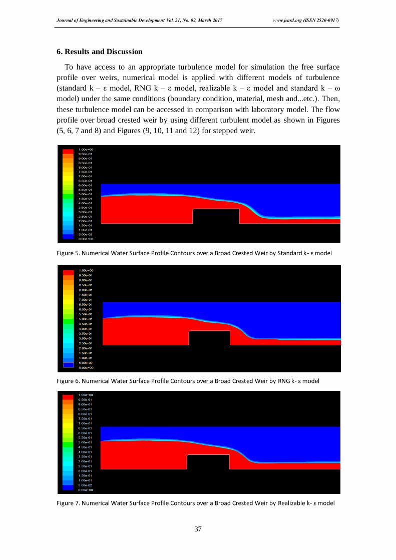
6. Results and Discussion

To have access to an appropriate turbulence model for simulation the free surface

profile over weirs, numerical model is applied with different models of turbulence

(standard k – ε model, RNG k – ε model, realizable k – ε model and standard k – ω

model) under the same conditions (boundary condition, material, mesh and...etc.). Then,

these turbulence model can be accessed in comparison with laboratory model. The flow

profile over broad crested weir by using different turbulent model as shown in Figures

(5, 6, 7 and 8) and Figures (9, 10, 11 and 12) for stepped weir.

Figure 5. Numerical Water Surface Profile Contours over a Broad Crested Weir by Standard k- ɛ model

Figure 6. Numerical Water Surface Profile Contours over a Broad Crested Weir by RNG k- ɛ model

Figure 7. Numerical Water Surface Profile Contours over a Broad Crested Weir by Realizable k- ɛ model


38

Figure 8. Numerical Water Surface Profile Contours over a Broad Crested Weir by standard k – ω model

Figure 9. Numerical Water Surface Profile Contours over a Stepped Weir by Standard k- ɛ model

Figure 10. Numerical Water Surface Profile Contours over a Stepped Weir by RNG k- ɛ model


39

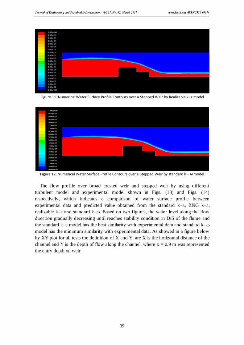
Figure 11. Numerical Water Surface Profile Contours over a Stepped Weir by Realizable k- ɛ model

Figure 12. Numerical Water Surface Profile Contours over a Stepped Weir by standard k – ω model

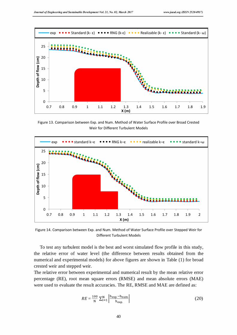
The flow profile over broad crested weir and stepped weir by using different

turbulent model and experimental model shown in Figs. (13) and Figs. (14)

respectively, which indicates a comparison of water surface profile between

experimental data and predicted value obtained from the standard k–ε, RNG k–ε,

realizable k–ε and standard k–ω. Based on two figures, the water level along the flow

direction gradually decreasing until reaches stability condition in D/S of the flume and

the standard k–ε model has the best similarity with experimental data and standard k–ω

model has the minimum similarity with experimental data. As showed in a figure below

by XY plot for all tests the definition of X and Y, are X is the horizontal distance of the

channel and Y is the depth of flow along the channel, where x = 0.9 m was represented

the entry depth on weir.


40

Figure 13. Comparison between Exp. and Num. Method of Water Surface Profile over Broad Crested

Weir for Different Turbulent Models

Figure 14. Comparison between Exp. and Num. Method of Water Surface Profile over Stepped Weir for

Different Turbulent Models

To test any turbulent model is the best and worst simulated flow profile in this study,

the relative error of water level (the difference between results obtained from the

numerical and experimental models) for above figures are shown in Table (1) for broad

crested weir and stepped weir.

The relative error between experimental and numerical result by the mean relative error

percentage (RE), root mean square errors (RMSE) and mean absolute errors (MAE)

were used to evaluate the result accuracies. The RE, RMSE and MAE are defined as:

𝑅𝐸 =

∑ |

|

(20)

0

5

10

15

20

25

0.7 0.8 0.9 1 1.1 1.2 1.3 1.4 1.5 1.6 1.7 1.8 1.9

De

pth

of

flo

w (

cm)

X (m)

exp Standard (k- ɛ) RNG (k-ɛ) Realizable (k- ɛ) Standard (k- ω)

0

5

10

15

20

25

0.7 0.8 0.9 1 1.1 1.2 1.3 1.4 1.5 1.6 1.7 1.8 1.9 2

De

pth

of

flo

w (

cm)

X (m)

exp standard k–ε RNG k–ε realizable k–ε standard k–ω


41

𝑅𝑀 𝐸 = √

∑

(21)

𝑀𝐴𝐸 =

∑ | |

(22)

Where; is the experimental head, is the numerical head, N is the total

number of points and i is the number of points. The relative error for broad crested weir

was about 5.11% to 13.1 % in RE, 0.39 % to 1.97 % in RMSE and 0.29 % to 1.86 % in

MAE. While, the relative error for stepped weir was about 3.54 % to 11.79 % in RE,

0.17 % to 1.59 % in RMSE and 0.149 % to 1.53 % in MAE.

Table 1. Relative Error of Water Level on Broad Crested Weir and Stepped Weir

Relative Error of Water level to Broad Crested Weir

Equation Turbulent

model MAE% RMSE% RE% 0.29 0.39 5.11 standard k–ε 0.36 0.43 5.25 RNG k–ε 1.08 1.23 8.37 realizable k–ε 1.86 1.97 13.1 standard k–ω

Relative Error of Water level to Stepped Weir Equation Turbulent

model MAE% RMSE% RE% 0.146 0.17 3.54 standard k–ε 0.35 0.39 4.63 RNG k–ε 0.8 0.83 7.86 realizable k–ε 1.53 1.59 11.79 standard k–ω

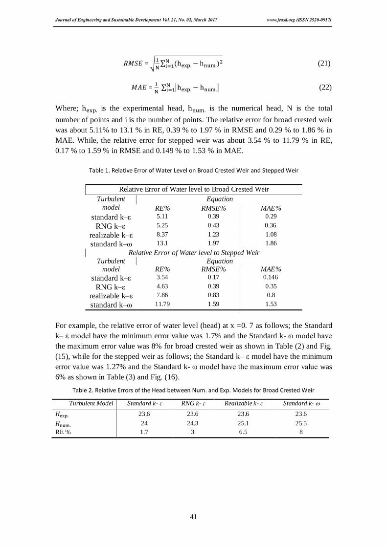
For example, the relative error of water level (head) at x =0. 7 as follows; the Standard

k– ε model have the minimum error value was 1.7% and the Standard k- ω model have

the maximum error value was 8% for broad crested weir as shown in Table (2) and Fig.

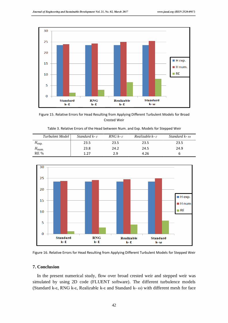
(15), while for the stepped weir as follows; the Standard k– ε model have the minimum

error value was 1.27% and the Standard k- ω model have the maximum error value was

6% as shown in Table (3) and Fig. (16).

Table 2. Relative Errors of the Head between Num. and Exp. Models for Broad Crested Weir

Turbulent Model Standard k- ɛ RNG k- ɛ Realizable k- ɛ Standard k- ω

23.6 23.6 23.6 23.6

24 24.3 25.1 25.5

RE % 1.7 3 6.5 8


42

Figure 15. Relative Errors for Head Resulting from Applying Different Turbulent Models for Broad

Crested Weir

Table 3. Relative Errors of the Head between Num. and Exp. Models for Stepped Weir

Turbulent Model Standard k- ɛ RNG k- ɛ Realizable k- ɛ Standard k- ω

23.5 23.5 23.5 23.5

23.8 24.2 24.5 24.9

RE % 1.27 2.9 4.26 6

Figure 16. Relative Errors for Head Resulting from Applying Different Turbulent Models for Stepped Weir

7. Conclusion

In the present numerical study, flow over broad crested weir and stepped weir was

simulated by using 2D code (FLUENT software). The different turbulence models

(Standard k-ε, RNG k-ε, Realizable k-ε and Standard k- ω) with different mesh for face


43

and edge can simulate the flow successfully. The VOF method was used to predict the

water surface profile. Results obtained in this study showed that the water level along

the flow direction gradually decreasing until reaches stability condition in D/S of the

flume and the comparison of water surface profile between experimental data and

predicted value obtained from the turbulent models showed that the standard k–ε model

has the best similarity with experimental data and standard k–ω model has the minimum

similarity with experimental data. The relative error of water level between

experimental and standard k–ε model for broad crested weir was 5.11% in RE and

standard k–ω was 13.1% in RE, while, the relative error of water level between

experimental and standard k–ε model for stepped broad crested weir was 3.54% in RE

and standard k–ω was 11.79% in RE. Also this study investigation the relative error of

water level at x =0. 7 and find the standard k– ε model have the minimum error value in

two weirs.

Abbreviations

A list of symbols that used in this research, shown in table below.

the coefficient of discharge

the experimental head

the numerical head the length of D/S step

the depth of water at the edge of the weir

the critical head

B width of the weir

E% the energy dissipation

Fr the dimensionless Froude number

H the head above weir crest with approach velocity (m) h, the head above weir crest without approach

velocity (m) L, the length of the weir

the height of the weir

height of step

R round edge of upstream edge

the actual discharge

the gravitational acceleration

8. References

1. Chow, V. T. (1959). "Open channel hydraulics", New York, McGraw-Hill, 1959.

2. Chanson H., (2001). "Hydraulic Design of Stepped Spillways and Downstream

Energy Dissipaters", Dam Engineering, Vol. 11, No. 4, pp. 205-242..

3. Boiten W., (2002). "Flow Measurement Structures", Wageningen University,

Wageningen, Gelderland, Netherlands, Flow Measurement and Instrumentation, Vol.

13, No. 5, pp. 203-207.

4. Bazin, (1896). "Open Channel Hydraulics", USA, McGraw-Hill,


44

5. Woodburn J. G., (1932). "Tests of Broad-Crested Weirs", Transactions of the

American Society of Civil Engineers, Vol. 96, No.1, pp. 417-453.

6. Hall G. W., (1962). "Discharge Characteristics of Broad-Crested Weirs Using

Boundary Layer Theory", London, England, Proceedings of the Institution of Civil

Engineers, pp. 172-190.

7. Ramamurthy A. S., Tim U. S., and Rao M. J., (1988). "Characteristics of Square-

Edged and Round-Nosed Broad-Crested Weirs", Journal of Irrigation and Drainage

Engineering, Vol. 114, No. 1, pp. 61-73.

8. Gonzalez, C. A., and Chanson, H. (2007). "Experimental measurements of velocity

and pressure distribution on a large broad-crested weir", Australia, Flow

Measurement and Instrumentation, Vol. 18, pp. 107–113.

9. Henderson F. M., (1966). "Open Channel Flow", New York, MacMillan.

10. Moss W. D., (1972). "Flow Separation at the Upstream of a Square-Edged Broad-

Crested Weir", Journal of Fluid Mechanics, Vol. 52, No. 2, pp. 307-320.

11. Hussein H. H., Juma A. and Shareef S., (2009). "Flow characteristics and energy

dissipation over stepped round–nosed broad–crested weirs", University of Mosul,

Journal of Al-Rafidain Engineering.

12. Hamid H., Inam A. K. and Saleh J. S., (2010). "Improving the Hydraulic

Performance of Single Step Broad-Crested Weirs", University of Mosul, Iraqi,

Journal of Civil Engineering, Vol. 7, No. 1, pp. 1-12.

13. Yazdi, J., Sarkardeh, H., Azamathulla, H.M., Ghani, A.A., (2010). "3D simulation of

flow around a single spur dike with free surface flow", Int. J. River Basin Manage.

No. 8 pp. 55-62.

14. Sarkar M. A. and Rhodes. D. G., (2004). "CFD and physical modeling of free surface

over broad-crested weir", Cranfield University, Swindon, pp. 215–219.

15. Hargreaves D. M., Morvan H. P. and Wright N. G., (2007). "Validation of the

Volume of Fluid Method for Free Surface Calculation: The Broad-Crested Weir",

The University of Nottingham, Engineering Applications of Computational Fluid

Mechanics, Vol. 1, No. 2, pp. 136–146.

16. Afshar H. and Hooman H., (2013), "Experimental and 3-D numerical simulation of

flow over a rectangular broad-crested weir", International Journal of Engineering and

Advanced Technology, Vol. 2, No. 6, pp. 214-219.

17. Hooman S., (2014). "3D Simulation Broad of Flow over a Triangular Broad-Crested

Weir", Journal of River Engineering, Vol. 2, No 2.

18. Seyed H. and Hossein A., (2014). "Flow over a Broad-Crested Weir in Subcritical

Flow Conditions, Physical Study", Journal of River Engineering, Vol. 2, No. 1.

19. Al-Hashimi A. S., Sadeq A. and Huda M., (2015). "Determination of Discharge

Coefficient of Rectangular Broad-Crested Weir by CFD", The 2nd International

Conference of Construction.

20. Dias, F., Keller, J.B., and Broeck,J.M, (1988). "Flows over rectangular weirs", Phys.

Fluids, No. 31, pp. 2071–2076.

21. Hager W. H. and Schwalt M., (1994). "Broad-crested weir", Journal of Irrigation and

Drainage Engineering, Vol. 120, No. 1, pp.13-26.


45

22. Hirt C. W. and Nichols B. D., (1981). "Volume of fluid (VOF) method for the

dynamics of free boundaries", Journal of Computational Physics, Vol. 39, No. 1, pp.

201-225.

23. Liu C, Hute A. and Wenju M., (2002). "Numerical and experimental investigation of

flow over a semicircular weir", Acta Mechanica Sinica, Vol. 18, pp. 594-602.

24. Lien F. S. and Leschziner M. A., (1994). "Assessment of turbulent transport models

including nonlinear RNG eddy-viscosity formulation and second-moment closure",

Computers and Fluids, Vol. 23, No. 8, pp. 983-1004.

25. Wilcox D. C., (1993). "Turbulence Modeling for CFD", DCW Industries Inc., La

Canada, California.

26. Launder B. and Spalding B. D., (1974). "The Numerical Computation of Turbulent

Flows", Computer Methods in Applied Mechanics and Engineering, No. 3.

27. Choudhury D., (1993). "Introduction to the Renormalization Group Method and

Turbulence Modeling", Fluent Inc. Technical Memorandum TM-107.

28. Shih T. H., Liou W., Shabbir A., and Zhu J., (1995). "A New k-ε Eddy-Viscosity

Model for High Reynolds Number Turbulent Flows - Model Development and

Validation", Computers Fluids, Vol. 24, No. 3, pp. 227-238.

29. Hirt C. W. and Nichols B. D., (1981). "Volume of fluid (VOF) method for the

dynamics of free boundaries", Journal of Computational Physics, Vol. 39, No. 1, pp.

201-225.

Documents

EXPERIMENTAL AND NUMERICAL SIMULATION OF FLOW OVER … · EXPERIMENTAL AND NUMERICAL SIMULATION OF FLOW OVER BROAD CRESTED WEIR AND STEPPED WEIR USING DIFFERENT TURBULENCE MODELS