Embed Size (px)
Citation preview
224 MP Proceedings of the 17th Int. AMME Conference, 19-21 April, 2016
17th International Conference on Applied Mechanics and Mechanical Engineering.
Military Technical College Kobry El-Kobbah,
Cairo, Egypt.
NUMERICAL ANALYSIS OF TURBULENT FLOW IN CENTRIFUGAL PUMP
S. M. Selim*, M. A. Hosien*, S. M. El-Behery*,1 and M. Elsherbiny*
ABSTRACT This paper presents numerical simulation of turbulent flow in centrifugal pump. Reynolds Averaged Navier-Stokes equations (RANS) are solved along with several turbulence models. The tested turbulence models ranged from two-equation turbulence model to the full Reynolds stress model (RSM). The rotation of the impeller is simulated according to moving and sliding mesh method provided by the computational fluid dynamics code, ANSYS Fluent 15. In addition, the effect of wall function approach on the simulated results is investigated. The numerical predictions are compared with experimental measurements form literature for radial and relative tangential velocity components at different locations within the tested pump. The comparison shows that the realizable k-ε predicts the flow within the pump with acceptable accuracy. Furthermore, the wall function has a negligible effect on the predicted results. Moreover, the results can predict some physical phenomena such as the pressure and velocity distribution along pressure and suction sides, blade loading, and rotor-stator interaction. KEYWORDS Numerical simulation, CFD, centrifugal pumps, turbulence models, moving and sliding mesh.
* Mechanical Power Engineering Department, Faculty of Engineering, Menoufyia University, Shebin El-Kom, Egypt.
1 Email: [email protected], Tel.:+201008002457.
225 MP Proceedings of the 17th Int. AMME Conference, 19-21 April, 2016
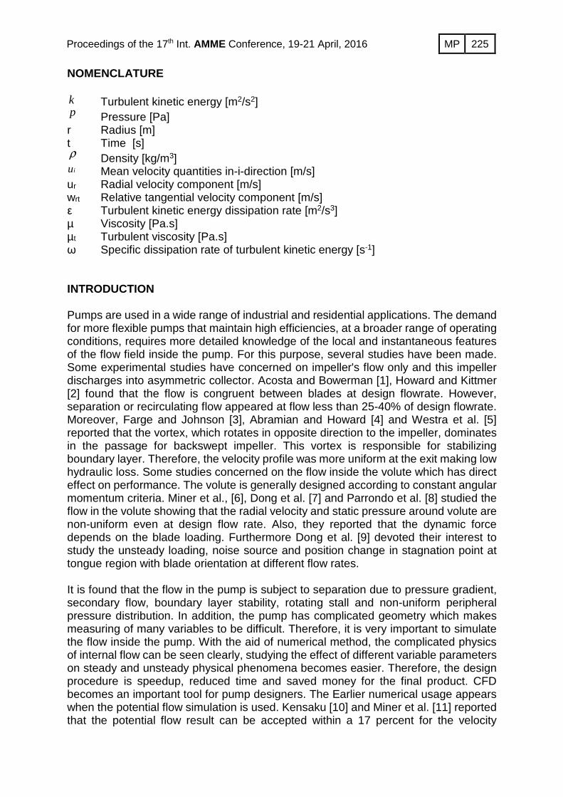
NOMENCLATURE k Turbulent kinetic energy [m2/s2] p Pressure [Pa] r Radius [m] t Time [s] ρ Density [kg/m3]
iu Mean velocity quantities in-i-direction [m/s] ur Radial velocity component [m/s] wrt Relative tangential velocity component [m/s] ε Turbulent kinetic energy dissipation rate [m2/s3] µ Viscosity [Pa.s] µt Turbulent viscosity [Pa.s] ω Specific dissipation rate of turbulent kinetic energy [s-1] INTRODUCTION Pumps are used in a wide range of industrial and residential applications. The demand for more flexible pumps that maintain high efficiencies, at a broader range of operating conditions, requires more detailed knowledge of the local and instantaneous features of the flow field inside the pump. For this purpose, several studies have been made. Some experimental studies have concerned on impeller's flow only and this impeller discharges into asymmetric collector. Acosta and Bowerman [1], Howard and Kittmer [2] found that the flow is congruent between blades at design flowrate. However, separation or recirculating flow appeared at flow less than 25-40% of design flowrate. Moreover, Farge and Johnson [3], Abramian and Howard [4] and Westra et al. [5] reported that the vortex, which rotates in opposite direction to the impeller, dominates in the passage for backswept impeller. This vortex is responsible for stabilizing boundary layer. Therefore, the velocity profile was more uniform at the exit making low hydraulic loss. Some studies concerned on the flow inside the volute which has direct effect on performance. The volute is generally designed according to constant angular momentum criteria. Miner et al., [6], Dong et al. [7] and Parrondo et al. [8] studied the flow in the volute showing that the radial velocity and static pressure around volute are non-uniform even at design flow rate. Also, they reported that the dynamic force depends on the blade loading. Furthermore Dong et al. [9] devoted their interest to study the unsteady loading, noise source and position change in stagnation point at tongue region with blade orientation at different flow rates. It is found that the flow in the pump is subject to separation due to pressure gradient, secondary flow, boundary layer stability, rotating stall and non-uniform peripheral pressure distribution. In addition, the pump has complicated geometry which makes measuring of many variables to be difficult. Therefore, it is very important to simulate the flow inside the pump. With the aid of numerical method, the complicated physics of internal flow can be seen clearly, studying the effect of different variable parameters on steady and unsteady physical phenomena becomes easier. Therefore, the design procedure is speedup, reduced time and saved money for the final product. CFD becomes an important tool for pump designers. The Earlier numerical usage appears when the potential flow simulation is used. Kensaku [10] and Miner et al. [11] reported that the potential flow result can be accepted within a 17 percent for the velocity
226 MP Proceedings of the 17th Int. AMME Conference, 19-21 April, 2016
magnitude at design condition. But, if the unsteady flow or off design condition are studied, poor results are obtained. The total governing equations must be solved with few assumptions in generalized coordinates for accurate results. The most acceptable method that deals with turbulent and gives the most accurate results is Direct Numerical Simulation (DNS). In this method, the time scale must be less than the fastest fluctuation in flow variables and grids must be finer than the smallest length scale. But, it takes more computational effort and needs computers with high specifications. Two approaches, Large Eddy Simulation (LES) and Reynold Averaged Navier-Stokes (RANS) are introduced to simplify the computational effort. Byskov et al. [12] simulate the flow in pump impeller using LES. No separation was observed at designed flow rate. While, steady non-rotating stall happens at quarter load. LES gives detailed predictions of the mean and fluctuation variables in 3D geometries. However, the computational costs still high. Many engineering application are interested in mean flow variables and a less computational cost approach is needed. The RANS method deals with time-average governed equations with aid of turbulence models. Gonzalez et al. [13] studied the capability of numerical method to capture the dynamic and unsteady flow effect inside pump. The sliding mesh technique with Standard k ε− model provided by the CFD code, FLUENT was used. Their results are in a good agreement with experimental data. Barrio et al. [14] estimated the performance of centrifugal pump and predicted the unsteady pressure distribution at the volute. Some turbulence models such as Spalart-Allmaras, standard k ε− , Reynold stress model (RSM) and standard k ω− were compared. They found that the standard k ε− can predict the flow field better than other models. Westra et al. [5] used the Spalart-Allmaras turbulence model to validate the numerical results via comparisons with the PIV results and good agreement between the results was reported. Liu et al. [15] studied the behavior of the flow and pressure fluctuation in centrifugal pump at shut-off condition. CFD code, CFX-11.0 was used to solve the unsteady RANS equations with SST k ω− turbulence model. The ability of numerical method using this turbulence model to predict this fluctuation was confirmed. Ayad et al. [16] investigated the effect of side clearance on the pump performance. The steady flow field is solved using multi-reference frame technique. They found that the pump heat and efficiency decreases as the side clearance increases. It can be seen from the previous discussions that there is no universal turbulence model accepted by all investigators for pump modelling. Therefore, the present paper aims to compare the performance of different turbulence models with different wall function approaches. MODEL DESCRIPTION AND COMPUTATIONAL METHOD The finite volume solver, ANSYS FLUENT 15 [17], solves the fully incompressible Reynolds averaged Navier-Stokes (RANS) equations with different available turbulence models. As the pump has a fixed domain (volute casing) and moving domain (impeller), FLUENT offers two solution techniques: Multi Reference Frame (MRF) and Sliding Mesh Modeled (SMM). The first one solves steady RANS equations in two domains related to subdomain's reference frame. This Technique is called frozen rotor approach as it freezes the motion of moving part in specific position. Therefore, the motion of blades relative to tongue is taken in to account. This method can be considered as the more realistic method. The time dependent term scheme is implicit second order and the coupled algorithm is used to calculate the pressure
227 MP Proceedings of the 17th Int. AMME Conference, 19-21 April, 2016
velocity coupling. Second order has been used for all variables (pressure, velocities and turbulence variables). Governing Equations
The flow in pumps can be considered as incompressible, isothermal and no reaction or mixing between fluid molecules. Governing equations that describe the flow in general form can be as follow [17]:
..V V V V
ddV wdA dA S dV
dt φρφ ρφ φ∂ ∂
+ = Γ∇ +∫ ∫ ∫ ∫r rr
where V is the control volume, V∂ is the boundary of control volume, Γ is the diffusion coefficient and Sφ is the source term of φ .
The Reynolds stress can be calculated directly using Reynolds Stress Mosel (RSM) or by the eddy viscosity models (EVM). In the later, the relation between the turbulent stresses (Reynolds stresses) and rate of strain through eddy viscosity based on Boussinesq assumption:
( )2
3ji
i j t ijj i
uuu u k
x xρ µ ρ δ
∂∂′ ′− = + − ∂ ∂
where 1ijδ = if i j= , 0ijδ = if i j≠ and k is turbulent kinetic energy.
A new parameter appears tµ which is known as turbulent (eddy) viscosity. Several models are available to calculate the eddy viscosity. These models are called Standard k-ε model: It was proposed by launder and spalding [18]. This model is widely in practical engineering and it calculates the eddy viscosity from the turbulent kinetic energy, k and its dissipation rate, ε. Realizable k-ε model: This model was proposed by shih et al. [19] as a modification of the standard k-ε model to satisfy certain mathematical constraints on Reynolds stresses according to the physics of turbulent flows which gives its name "realizable". Modifications depend on turbulent viscosity and the dissipation rate equation. The 2v f′ − model: The 2v f′ − Model Is Considered Low-Reynolds Number Turbulence model, so it doesn’t need to use wall function. In this model, a transport equation for ��� and an elliptic relaxation equation for f are solved in addition to the well-known k and ε equations. More details about this model can be found in Durbin [20]. Shear-Stress Transport k ω− (Sst k ω− ) model: This Hybrid Model Combines The robust and accurate formulation in the near-wall region of k-ω model the with the free stream independence of the k-ε model in the far field. The transition from k-ω model to k-ε model is achieved through blending functions developed by Menter [21].
228 MP Proceedings of the 17th Int. AMME Conference, 19-21 April, 2016
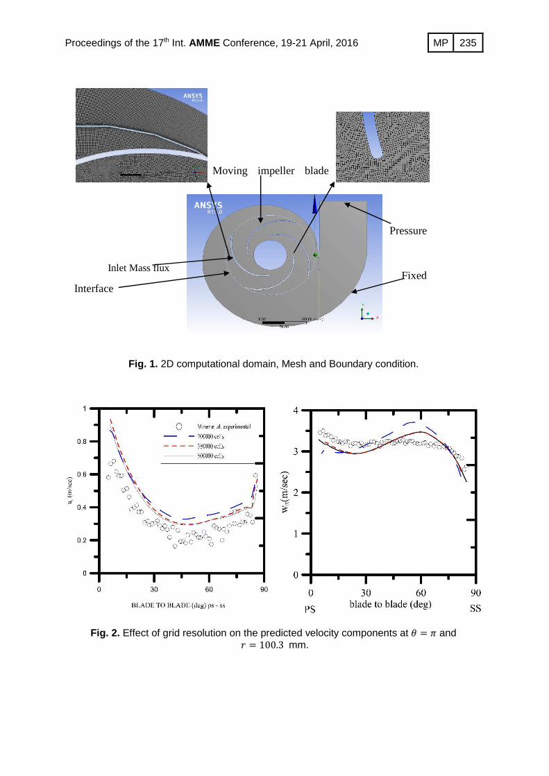
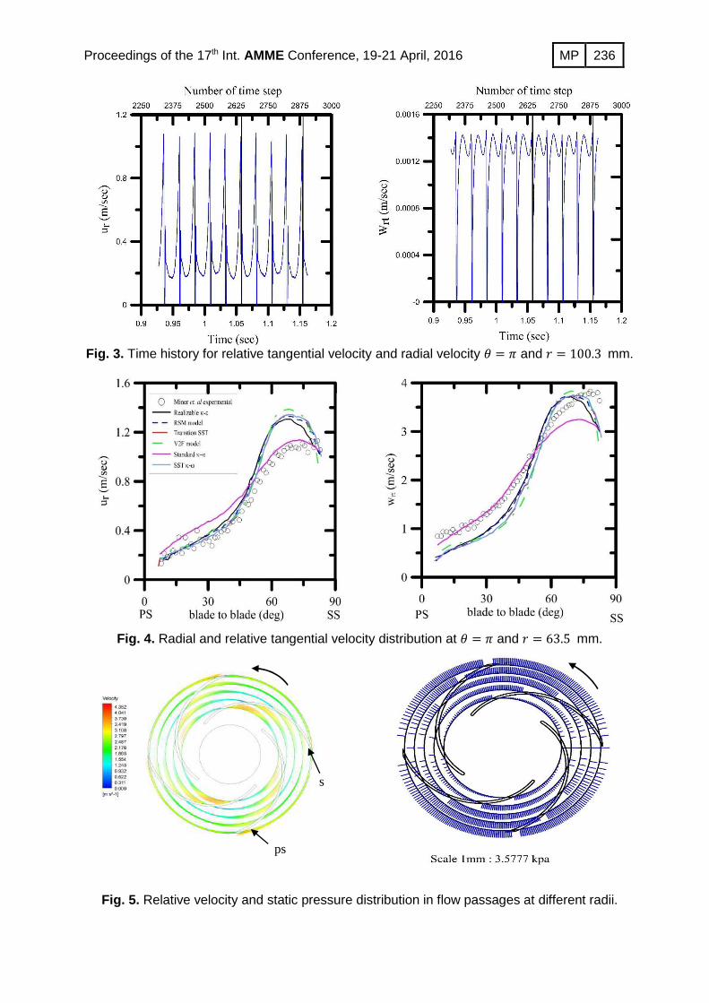
Transition SST model: The transition from laminar to turbulent is generally predicted by low Reynolds number turbulence models, where the wall damping functions trigger the transition onset. The transition SST model is an alternate to the low-Re turbulence model. Menter et al. [22] developed two transport equations, one for intermittency factor and one for the transition onset criteria in terms of momentum thickness Reynolds number. The intermittency is introduced in the SST k ω− through the production term. Reynolds stress model (RSM): Unlike the aforementioned models which relates the Reynolds-stress tensor to the strain-rate tensor through the eddy viscosity, the RSM model solves a separate transport equation for each component of Reynolds stresses. Detailed description of this model can be found in [23]. Computational Domain and Boundary Conditions Miner and co-workers [6, 11] measured the velocity components on pump at points using Laser Doppler Velocimeter (LDV). Tested pump has constant elevation in the third dimension. They preferred this geometry to study the uncertainty range of results predicted by a two dimensional potential flow analysis as reported in Miner et al. [11]. The agreement between experimental results and prediction by potential flow theory was poor. The probability of study this pump with 2D viscous governing equations is our interest. Consequently, the two dimensional pump has been designed and tested with different turbulence models and different wall functions. The pump specifications are given in Table 1. The 2D geometry is modeled by ANSYS Design Modeler. The moving and stationary parts are separated zones. Quadrilateral cells in the total domain are generated by using ANSYS Meshing. Three different computational mesh of different number of cells are tested. These meshes contains 20000, 38000 and 500000 cells, respectively. Comparisons between predicted results using the three grids shows that there is no noticeable differences between the coarser and intermediate grid, as shown in Fig. 1. Therefore, the computational grid 380000 cells is used for simulation to reduce the computational cost. A view of the pump with different mesh sections is shown in Fig. 2. Several types of boundary conditions are used in the current simulation. At the wall. No-slip boundary conditions are specified with wall function approach, while at inlet specified mass flux of 1067kg/m2.s is used. This mass flux corresponds to the design flow rate. At the outlet, pressure outlet boundary condition with gage pressure of 0.178 bar is applied. Details of boundary conditions are shown also in Fig. 2. Near-Wall Treatment Generally, there are two approaches to model the wall effect in turbulent flow. The first approach is to use very fine grid to locate the first near-wall grid point I the viscous sublayer (y+ ≈ 1) and integrate the flow equation directly to the wall. The second approach uses semi-empirical formulas called wall functions are used to bridge the viscosity-affected region between the wall and the fully turbulent region. In complex geometries such as centrifugal pumps with many recirculation zones it difficult to locate the first near-wall grid point in the viscous sublayer. Therefore, the use of wall function
229 MP Proceedings of the 17th Int. AMME Conference, 19-21 April, 2016
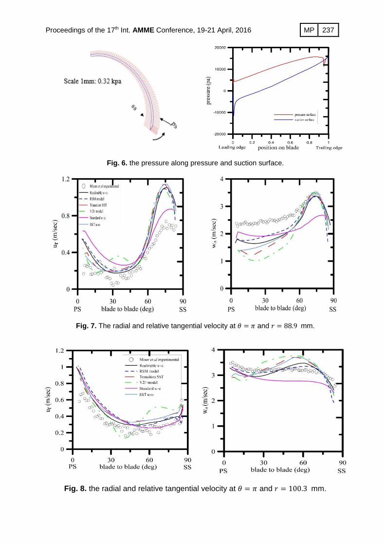
approach is recommended. Four wall-function approaches are examined in the present study. Details of these wall functions can be found in [17]. Solution Procedure Firstly, a converged steady state solution is obtained using the multi-reference frame technique. This converged solution is used as the initial estimation for the unsteady solution with sliding mesh technique. The converged solution is accepted when the sum of normalized residuals of all flow variable becomes less than 10-5. Time step used in the unsteady calculation adjusted to be lower than the time the time period taken by blade thickness at the outer periphery. The calculated time step equals 4×10⁻⁴ s. Therefore, a complete revolution is performed each 242 time steps. The radial and relative tangential velocities are monitored at the points several point for comparison with experimental data. After several time steps, the flow becomes periodic, as shown in Fig. 3. The periodic flow results are stored for complete revolution and averaged for comparison for experimental data. RESULTS AND DISCUSSIONS The first point used in calculations is the point at angle � = � (side at the same level with center of rotation and opposite to the tongue) at a radius equals to 63.5 mm. The measured and predicted values for radial and relative tangential velocity for various turbulence models at this point are shown in Fig.4. The different turbulence models have similar trends in predicting the velocity components at the first point as seen in Fig.4. The standard k ε− model predicts the relative tangential velocity well at the pressure side and under-predicts it at the suction side. Other tested models under-predict the relative tangential velocity at the pressure side and predict it fairly good at the suction side. For the radial velocity, the standard k ε− model over-predicts it at the pressure side while other models over-predicts it at the suction side. Also, the standard k ε− expects the blade loading lower than that expected from the others but it has the best trend for velocity profile. It can be seen from experimental results that the relative and radial velocities are lower at the pressure side than at the other side (suction side). Tuzson [24] defined the pressure side as the side facing the flow in the direction of rotation. The difference in the value of the square relative velocity magnitude on both sides is caused by the difference in the pressure as governed by Rothalpy equation. According to Wislicenus [25], Rothalpy equation "or relative energy equation" can be considered as a relationship equivalent to Bernoulli's equation applied in rotating impeller. The
mathematical form for this equation can be written as ( )
22
2 2r
rp WI losses
g g g
ω
ρ= + − − .
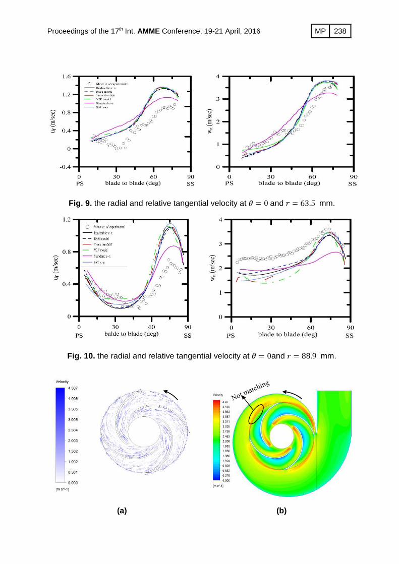
Consequently, at the same radius, when the static pressure head h increased, the relative velocity decreased. The pressure difference between the two sides of the blade (pressure and suction side) is called Blade loading. The larger the pressure difference is, the larger the blade loading becomes. The 2D simulation illustrates this physical phenomenon. This can be illustrated by determining the pressure and relative velocity
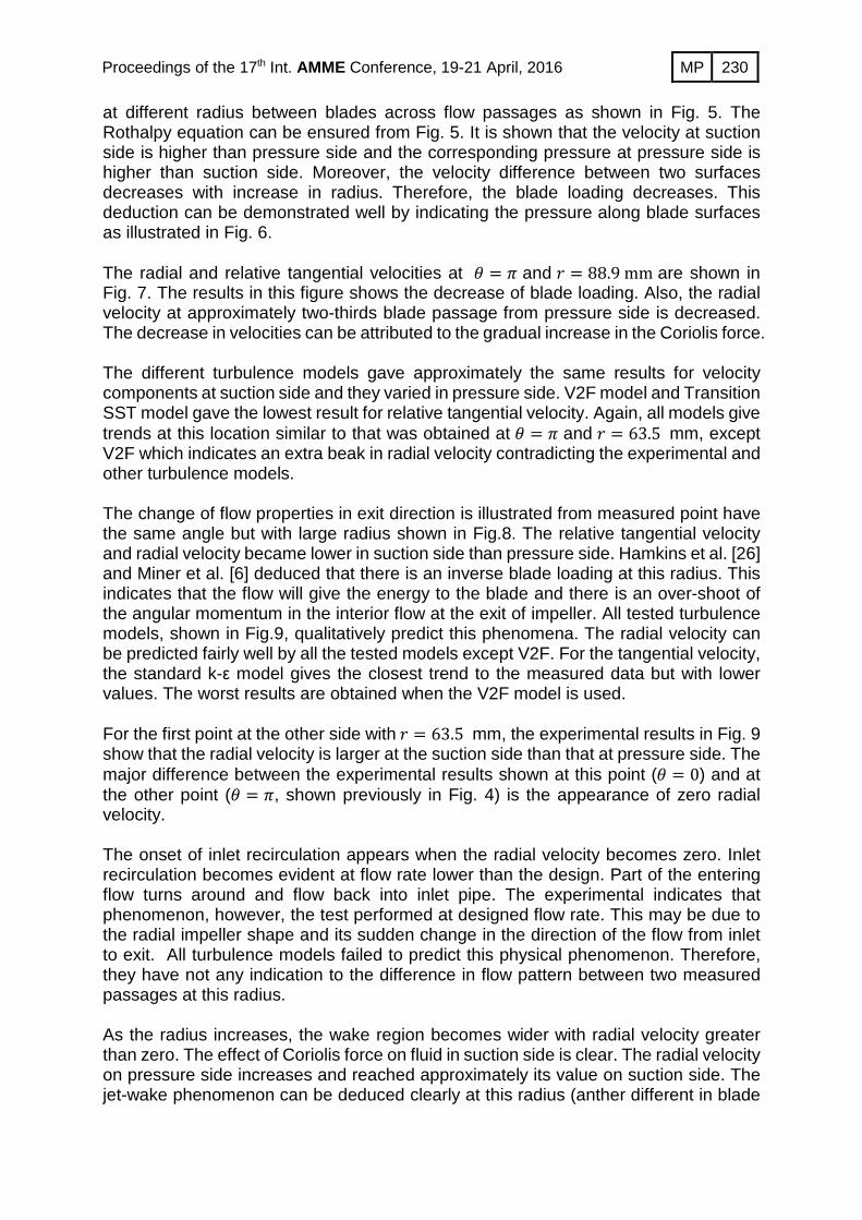
230 MP Proceedings of the 17th Int. AMME Conference, 19-21 April, 2016
at different radius between blades across flow passages as shown in Fig. 5. The Rothalpy equation can be ensured from Fig. 5. It is shown that the velocity at suction side is higher than pressure side and the corresponding pressure at pressure side is higher than suction side. Moreover, the velocity difference between two surfaces decreases with increase in radius. Therefore, the blade loading decreases. This deduction can be demonstrated well by indicating the pressure along blade surfaces as illustrated in Fig. 6. The radial and relative tangential velocities at � = � and � = 88.9mm are shown in Fig. 7. The results in this figure shows the decrease of blade loading. Also, the radial velocity at approximately two-thirds blade passage from pressure side is decreased. The decrease in velocities can be attributed to the gradual increase in the Coriolis force. The different turbulence models gave approximately the same results for velocity components at suction side and they varied in pressure side. V2F model and Transition SST model gave the lowest result for relative tangential velocity. Again, all models give trends at this location similar to that was obtained at � = � and � = 63.5 mm, except V2F which indicates an extra beak in radial velocity contradicting the experimental and other turbulence models. The change of flow properties in exit direction is illustrated from measured point have the same angle but with large radius shown in Fig.8. The relative tangential velocity and radial velocity became lower in suction side than pressure side. Hamkins et al. [26] and Miner et al. [6] deduced that there is an inverse blade loading at this radius. This indicates that the flow will give the energy to the blade and there is an over-shoot of the angular momentum in the interior flow at the exit of impeller. All tested turbulence models, shown in Fig.9, qualitatively predict this phenomena. The radial velocity can be predicted fairly well by all the tested models except V2F. For the tangential velocity, the standard k-ε model gives the closest trend to the measured data but with lower values. The worst results are obtained when the V2F model is used. For the first point at the other side with� = 63.5 mm, the experimental results in Fig. 9 show that the radial velocity is larger at the suction side than that at pressure side. The major difference between the experimental results shown at this point (� = 0) and at the other point (� = �, shown previously in Fig. 4) is the appearance of zero radial velocity. The onset of inlet recirculation appears when the radial velocity becomes zero. Inlet recirculation becomes evident at flow rate lower than the design. Part of the entering flow turns around and flow back into inlet pipe. The experimental indicates that phenomenon, however, the test performed at designed flow rate. This may be due to the radial impeller shape and its sudden change in the direction of the flow from inlet to exit. All turbulence models failed to predict this physical phenomenon. Therefore, they have not any indication to the difference in flow pattern between two measured passages at this radius. As the radius increases, the wake region becomes wider with radial velocity greater than zero. The effect of Coriolis force on fluid in suction side is clear. The radial velocity on pressure side increases and reached approximately its value on suction side. The jet-wake phenomenon can be deduced clearly at this radius (anther different in blade

231 MP Proceedings of the 17th Int. AMME Conference, 19-21 April, 2016
passages) as illustrated from radial velocity shown in Fig.10. The blade loading is reduced as the difference between relative velocities across the blade decreased. All turbulence models predict the increase in wake region and the decrease in blade loading at this radius than previous one. The experimental results shown before indicate that the properties in two-measured passage at the largest measured radius are approximately similar for both radial and relative tangential velocity components in their trend and their values. From the previous results, it is clear that the turbulence models vary in their prediction. One model gives better prediction at some points and another gives better at different points. A statistical analysis is needed to determine the most accurate turbulence model, which gives the mean prediction results closer to physical real flow. The mean deviation error ME between predicted and experimental results for the
tested turbulence models is calculated by exp
1 exp
1 i nnum
i
U UME abs
n U
=
=
−=
∑ . The value of
exp,numU U should be at the same angle. In order to have the corresponding value of
numerical result at certain angle determined from experimental data, Basic program is made. The program interpolates between the closest numerical angles to give the desired numerical result. The statistical deviation results of radial and tangential velocities at six measuring points for each turbulence model are shown in Tables 2 and 3. The result in table demonstrate the realizable k-ε model predict results with the smallest deviation and the largest deviation is given by V2F. From Tables 2 and 3, it is noticed that the maximum deviation for all turbulence models occurs at the closest measured point from inlet pipe in tongue direction� = 0, � = 63.5. However, the minimum deviation for them occurs at counterpart point. The standard k-ε model gives the lowest deviation for measured outer points near the tongue� = �, � = 88.9, � = 100.3 mm. Table 4 shows the mean deviation error for both velocity components. The results in this table show that the lowest mean deviation is given by realizable k ε− model and the V2F model drops from turbulence competition. A complete picture of the flow through the centrifugal pump is shown in Fig.11. The relative velocity vectors (seen from observer moving with impeller) is shown in Fig.11-a. It can be seen from this figure that the flow mostly follows the blades. On the other hand, the absolute velocity (seen from stationary observer) vectors, shown in Fig.11-c, show that the flow is totally rotates with impeller. Due to the relative motion between the blades and the flow, the fluid particles impinge the convex surface of the blade and keep the concave surface away. As a result, the pressure increases at convex surface (pressure side) and decrease at the concave surface (suction side) as shown in Fig.11-d. According to relative energy equation the relative tangential velocity increases at the suction side and decreases in the other, Fig.11-d. While the flow passes through the impeller, the energy transfers from the rotor to the fluid. Consequently, the fluid velocity and pressure increase through the impeller. However, the velocity decreases in the volute due to gradual change in area and pressure increases (energy transformation) as cleared in Fig.11-d, e.
232 MP Proceedings of the 17th Int. AMME Conference, 19-21 April, 2016
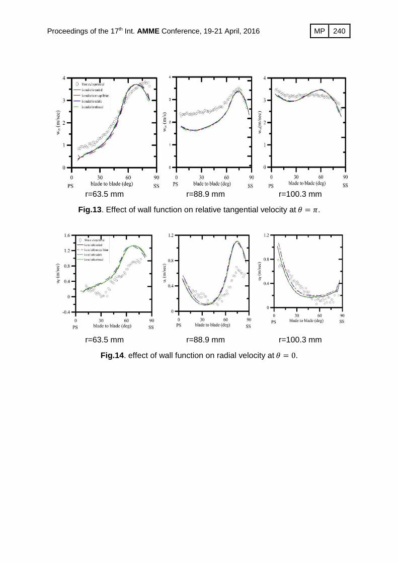
The effect of different wall treatment on the predicted velocity profile is shown in Figs. 12-14. It can be seen from these figures that the wall function has minor effect on the predicted results. CONCLUSION Unsteady Turbulent flow in centrifugal pump has been simulated using sliding mesh technique. Different turbulence models has been tested and evaluated against measured velocity components in a model pump. Despite the simplified geometry of the tested pump (constant width), none of the tested turbulence models can predicts quantitatively the correct velocity behavior. They can only predict the qualitative flow behavior. Statistical analysis of model performance in terms of mean square error, MSE showed that the Realizable k ε− can predict better results than other tested models. In addition, different wall functions has been tested and they didn't indicate any difference in predicted results. REFERENCES
[1] Acosta, A.J. and Bowerman, R.D., 1957. An experimental study of centrifugal-pump impellers. Transactions of the ASME, 79(4), pp.1821-1839.
[2] Howard, J.H.G. and Kittmer, C.W., 1975. Measured passage velocities in a radial impeller with shrouded and unshrouded configurations. Journal of Engineering for Power, 97(2), pp.207-212.
[3] Farge, T.Z. and Johnson, M.W., 1992. Effect of flow rate on loss mechanisms in a backswept centrifugal impeller. International journal of heat and fluid flow, 13(2), pp.189-196.
[4] Abramian, M. and Howard, J.H.G., 1994. Experimental investigation of the steady and unsteady relative flow in a model centrifugal impeller passage.Journal of turbomachinery, 116(2), pp.269-279.
[5] Westra, R.W., Broersma, L., Van Andel, K. and Kruyt, N.P., 2010. PIV measurements and CFD computations of secondary flow in a centrifugal pump impeller. Journal of Fluids Engineering, 132(6), p.061104.
[6] Miner, S.M., Beaudoin, R.J. and Flack, R.D., 1989. Laser velocimeter measurements in a centrifugal flow pump. Journal of turbo machinery, 111(3), pp.205-212.
[7] Dong, R., S. Chu, and J. Katz. "Quantitative visualization of the flow within the volute of a centrifugal pump. Part B: results and analysis." Journal of fluids engineering 114.3 (1992): 396-403.
[8] Stickland, M.T., Scanlon, T.J., Parrondo, J., González-Pérez, J. and Fernández-Francos, J., 2000. An experimental study on the unsteady pressure distribution around the impeller outlet of a centrifugal pump. In Proceedings of ASME, Boston, Massachusett, FEDSM00–11302.
[9] Dong, R., Chu, S. and Katz, J., 1997. Effect of modification to tongue and impeller geometry on unsteady flow, pressure fluctuations, and noise in a centrifugal pump. Journal of Turbomachinery. Transactions of the ASME, 119(3), pp.506-515.
233 MP Proceedings of the 17th Int. AMME Conference, 19-21 April, 2016
[10] Imaichi, K., Tsujimoto, Y., Yoshida, Y. and MIZUTANI, H., 1980. A Two-Dimensional Analysis of the Interaction Effects of Radial Impeller in Volute Casing. In Proceedings of the 10th lAHR Symposium (pp. 635-647).
[11] Miner, S.M., Flack, R.D. and Allaire, P.E., 1992. Two-Dimensional Flow Analysis of a Laboratory Centrifugal Pump. Journal of Turbomachinery, 114, pp.333-339.
[12] Byskov, R.K., Jacobsen, C.B. and Pedersen, N., 2003. Flow in a centrifugal pump impeller at design and off-design conditions: Part II: Large eddy simulations. Journal of fluids engineering, 125(1), pp.73-83.
[13] Gonzalez, J., Fernández, J., Blanco, E. and Santolaria, C., 2002. Numerical simulation of the dynamic effects due to impeller-volute interaction in a centrifugal pump. Journal of Fluids Engineering, 124(2), pp.348-355.
[14] Barrio, R., Parrondo, J. and Blanco, E., 2010. Numerical analysis of the unsteady flow in the near-tongue region in a volute-type centrifugal pump for different operating points. Computers & Fluids, 39(5), pp.859-870.
[15] Liu, H., Wu, X. and Tan, M., 2013. Numerical investigation of the inner flow in a centrifugal pump at the shut-off condition. Journal of Theoretical and Applied Mechanics, 51, pp. 649-660.
[16] Ayad, A.F., Abdalla, H.M. and Aly, A.A.E.A., 2015. Effect of semi-open impeller side clearance on the centrifugal pump performance using CFD. Aerospace Science and Technology, 47, pp.247-255.
[17] FLUENT 15 theory guide, ANSYS Inc., 2013. [18] Launder, B.E. and Spalding, D.B., 1974. The numerical computation of
turbulent flows. Computer methods in applied mechanics and engineering,3(2), pp.269-289.
[19] Shih, T.H., Liou, W.W., Shabbir, A., Yang, Z. and Zhu, J., 1995. A new k-ϵ eddy viscosity model for high Reynolds number turbulent flows. Computers & Fluids, 24(3), pp.227-238.
[20] Durbin, P.A., 1991. Near-wall turbulence closure modeling without “damping functions”. Theoretical and Computational Fluid Dynamics, 3(1), pp.1-13.
[21] Menter, F.R., 1994. Two-equation eddy-viscosity turbulence models for engineering applications. AIAA journal, 32(8), pp.1598-1605.
[22] Menter, F.R., Langtry, R.B., Likki, S.R., Suzen, Y.B., Huang, P.G. and Völker, S., 2006. A correlation-based transition model using local variables—part I: model formulation. Journal of turbomachinery, 128(3), pp.413-422.
[23] Launder B. E., Spalding D. B., 1972. Mathematical Models of Turbulence. Lecture notes, Imperial College of Science and Technology.
[24] Tuzson J., 2000. Centrifugal Pump Design. JOHN WILEY & SONS, INC. [25] Wisclicenus G. F., 1965. Fluid Mechanics of Turbomachinery" Vol. 2, Dover,
New York, P. 626. [26] Hamkins, C.P. and Flack, R.D., 1987. Laser velocimeter measurements in
shrouded and unshrouded radial flow pump impellers. Journal of turbomachinery, 109(1), pp.70-76.
234 MP Proceedings of the 17th Int. AMME Conference, 19-21 April, 2016
Table 1 pump specification.
Inlet diameter
[mm]
Duct outlet [mm]
Blades number
Blades thickness
[mm]
Pump width [mm]
pump speed [rpm]
Design flowrate
[L/s]
Design head [N/m2]
76.2 108 4 3 24.6 620 6.3 L/s 17800
Table 2. The mean deviation error of radial velocity for the tested turbulence models.
(θ, r) Realizable
k ε− Standard
k ε− RSM Transition
SST V2F SST
k ω− π, 63.5 0.176965 0.225235 0.161975 0.150221 0.179554 0.150887 π, 88.9 0.6035227 0.9503416 0.738741 0.668557 0.9108031 0.6236044 π, 100.3 0.3057312 0.3010596 0.3815238 0.4177482 0.4467944 0.4131406 0, 63.5 0.9215938 1.186426 0.92276 0.9388384 0.9578963 0.9710429 0, 88.9 0.5033041 0.4036085 0.4772774 0.5569603 0.5620682 0.5353454 0, 100.3 0.4265997 0.3773147 0.3938684 0.6786527 0.9647629 0.6137226 Mean 0.4896193 0.5739975 0.512691 0.568496 0.6703131 0.5512906
Table 3. The mean deviation error of relative tangential velocity for the tested turbulence models.
(θ, r) Realizable
k ε− Standard
k ε− RSM Transition
SST V2F SST k ω−
π, 63.5 0.1892675 7.88E-02 0.1951143 0.2164662 0.2139679 0.2128184 π, 88.9 0.1982343 0.2031916 0.15608 0.2708506 0.3260067 0.2276849 π, 100.3 5.61E-02 0.113726 0.0521031 9.96E-02 0.1236189 9.29E-02 0, 63.5 0.2360396 0.16396 0.2448934 0.2193465 0.1734126 0.2297687 0, 88.9 0.1915493 0.2318686 0.1604899 0.2240341 0.2754728 0.2254601
0, 100.3 6.99E-02 0.1365465 7.28E-02 0.1111193 0.1339729 0.105132 Mean 0.1568387 0.154683 0.1469216 0.1902412 0.2077419 0.1822997
Table 4. The total mean deviation for each tested turbulence model.
Realizable
k ε− Standard
k ε− RSM Transition SST V2F SST k ω−
Total mean
0.3232290
0.364340
0.3298063
0.3793687
0.4390275
0.3667951
235 MP Proceedings of the 17th Int. AMME Conference, 19-21 April, 2016
Fig. 1. 2D computational domain, Mesh and Boundary condition.
Fig. 2. Effect of grid resolution on the predicted velocity components at � = � and � = 100.3 mm.
Inlet Mass flux
Moving impeller blade
Interface Fixed
Pressure
236 MP Proceedings of the 17th Int. AMME Conference, 19-21 April, 2016
Fig. 3. Time history for relative tangential velocity and radial velocity � = � and � = 100.3 mm.
Fig. 4. Radial and relative tangential velocity distribution at � = � and � = 63.5 mm.
Fig. 5. Relative velocity and static pressure distribution in flow passages at different radii.
ps
s
237 MP Proceedings of the 17th Int. AMME Conference, 19-21 April, 2016
Fig. 6. the pressure along pressure and suction surface.
Fig. 7. The radial and relative tangential velocity at � = � and � = 88.9 mm.
Fig. 8. the radial and relative tangential velocity at � = � and � = 100.3 mm.
238 MP Proceedings of the 17th Int. AMME Conference, 19-21 April, 2016
Fig. 9. the radial and relative tangential velocity at � = 0and � = 63.5 mm.
Fig. 10. the radial and relative tangential velocity at � = 0and � = 88.9 mm.
(a) (b)
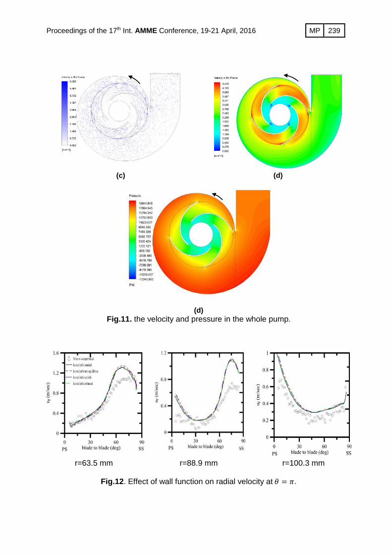
239 MP Proceedings of the 17th Int. AMME Conference, 19-21 April, 2016
(c) (d)
(d) Fig.11. the velocity and pressure in the whole pump.
r=63.5 mm r=88.9 mm r=100.3 mm
Fig.12. Effect of wall function on radial velocity at� = �.
240 MP Proceedings of the 17th Int. AMME Conference, 19-21 April, 2016
r=63.5 mm r=88.9 mm r=100.3 mm
Fig.13. Effect of wall function on relative tangential velocity at� = �.
r=63.5 mm r=88.9 mm r=100.3 mm
Fig.14. effect of wall function on radial velocity at� = 0.