Embed Size (px)
Citation preview

High-Resolution Numerical Simulation of
Turbulent Interfacial Marine Flows
by
Grzegorz P. Filip
A dissertation submitted in partial fulfillmentof the requirements for the degree of
Doctor of Philosophy(Naval Architecture and Marine Engineering)
in the University of Michigan2013
Doctoral Committee:
Professor Kevin J. Maki, ChairProfessor Luis P. BernalSung-Eun Kim, NSWC CarderockProfessor Armin W. TroeschProfessor Yin Lu Young

“A society grows great when old men plant trees in whose shade they know theyshall never sit.”
– Greek proverb

©Grzegorz P. Filip
2013

Dedicated to my family.
ii
ACKNOWLEDGMENTS
I would like to give special thanks to Prof. Kevin Maki for his guidance and
friendship, and to my committee members, Prof. Luis Bernal, Dr. Sung-Eun Kim,
Prof. Armin Troesch, and Prof. Yin Lu Young.
I want to thank my family, especially my parents, Adam and Irena, for their
continuous encouragement and support. Special thanks to all my friends who made
this endeavor a very memorable part of my life.
This dissertation was funded by the Department of Defense via the National De-
fense Science and Engineering Graduate (NDSEG) fellowship and it is gratefully
acknowledged together with the additional support from the US Office of Naval Re-
search (ONR) grants N00014-10-1-0301 and N00014-11-1-0846.
I would like to acknowledge the Extreme Science and Engineering Discovery En-
vironment (XSEDE), which is supported by National Science Foundation grant num-
ber OCI-1053575, and the Computer Aided Engineering Network High Performance
Computing (CAEN HPC) Group at the University of Michigan.
iii
TABLE OF CONTENTS
DEDICATION . . . . . . . . . . . . . . . . . . . . . . . . . . . . . . . . . . ii
ACKNOWLEDGMENTS . . . . . . . . . . . . . . . . . . . . . . . . . . . iii
LIST OF FIGURES . . . . . . . . . . . . . . . . . . . . . . . . . . . . . . . vi
LIST OF TABLES . . . . . . . . . . . . . . . . . . . . . . . . . . . . . . . . ix
ABSTRACT . . . . . . . . . . . . . . . . . . . . . . . . . . . . . . . . . . . x
CHAPTER
1 Introduction . . . . . . . . . . . . . . . . . . . . . . . . . . . . . . . . . . 1
2 Background and Related Work . . . . . . . . . . . . . . . . . . . . . . 7
2.1 Simulation of Interfacial Marine Flows . . . . . . . . . . . . . . . . 72.2 Overview of Large-Eddy Simulations . . . . . . . . . . . . . . . . . 11
2.2.1 Filtering of the Governing Equations . . . . . . . . . . . . . 122.2.2 Subgrid-Scale Stress Closure Models . . . . . . . . . . . . . 17
2.3 Large-Eddy Simulations of Interfacial Flows . . . . . . . . . . . . . 252.3.1 Governing Equations . . . . . . . . . . . . . . . . . . . . . . 262.3.2 Role of Subgrid Scales . . . . . . . . . . . . . . . . . . . . . 29
3 Direct Numerical Simulations of Canonical Interfacial Flows . . . 33
3.1 Numerical Method . . . . . . . . . . . . . . . . . . . . . . . . . . . 343.1.1 Solution Procedure . . . . . . . . . . . . . . . . . . . . . . . 353.1.2 Filtering Operation . . . . . . . . . . . . . . . . . . . . . . . 363.1.3 Validation of the A Priori Procedure . . . . . . . . . . . . . 37
3.2 Phase Inversion . . . . . . . . . . . . . . . . . . . . . . . . . . . . . 393.2.1 Quantification of the Subgrid Contributions . . . . . . . . . 423.2.2 Modeling of the Subgrid-Scale Terms . . . . . . . . . . . . . 52
3.3 Plunging-Breaking Wave . . . . . . . . . . . . . . . . . . . . . . . . 603.3.1 Validation Study . . . . . . . . . . . . . . . . . . . . . . . . 633.3.2 Results and Discussion . . . . . . . . . . . . . . . . . . . . . 653.3.3 Quantification of the Subgrid Contributions . . . . . . . . . 693.3.4 Modeling of the Subgrid-Scale Terms . . . . . . . . . . . . . 76
3.4 Summary . . . . . . . . . . . . . . . . . . . . . . . . . . . . . . . . 82
iv

4 Large-Eddy Simulations of Turbulent Interfacial Marine Flows . . 84
4.1 Modeling Multiphase Subgrid Contributions . . . . . . . . . . . . . 854.2 Phase Inversion . . . . . . . . . . . . . . . . . . . . . . . . . . . . . 86
4.2.1 Total Kinetic Energy . . . . . . . . . . . . . . . . . . . . . . 884.2.2 Kinetic Energy Dissipation Rate . . . . . . . . . . . . . . . . 91
4.3 Plunging-Breaking Wave . . . . . . . . . . . . . . . . . . . . . . . . 974.3.1 Kinetic Energy and Energy Dissipation . . . . . . . . . . . . 984.3.2 Interfacial Subgrid-Scale Contribution . . . . . . . . . . . . 100
4.4 Cylinder in Waves . . . . . . . . . . . . . . . . . . . . . . . . . . . . 1024.4.1 Problem Description . . . . . . . . . . . . . . . . . . . . . . 1034.4.2 Linear Regular Waves . . . . . . . . . . . . . . . . . . . . . 1064.4.3 Steep Regular Waves . . . . . . . . . . . . . . . . . . . . . . 1084.4.4 Steep Regular Waves and Modeling of Interfacial Turbulence 114
4.5 Summary . . . . . . . . . . . . . . . . . . . . . . . . . . . . . . . . 122
5 Summary and Conclusions . . . . . . . . . . . . . . . . . . . . . . . . . 124
5.1 Summary . . . . . . . . . . . . . . . . . . . . . . . . . . . . . . . . 1245.2 Contributions . . . . . . . . . . . . . . . . . . . . . . . . . . . . . . 1275.3 Future Work . . . . . . . . . . . . . . . . . . . . . . . . . . . . . . . 129
BIBLIOGRAPHY . . . . . . . . . . . . . . . . . . . . . . . . . . . . . . . . 131
v

LIST OF FIGURES
1.1 Experimental study of plunging-breaking wave impacts on an offshorewind turbine platform . . . . . . . . . . . . . . . . . . . . . . . . . . . . 2
1.2 Energy spectrum of turbulent flows . . . . . . . . . . . . . . . . . . . . . 4
2.1 Illustration of low-pass filtering in one dimension using a top-hat filter . 142.2 True SGS stress (far left) in an open-jet flow compared to the modeled
stress using the Smagorinsky model (middle) and the stress-similarity (farright) models . . . . . . . . . . . . . . . . . . . . . . . . . . . . . . . . . 23
3.1 Subgrid-scale stress components for the fully-developed turbulent channelflow (Reτ = 171) . . . . . . . . . . . . . . . . . . . . . . . . . . . . . . . 38
3.2 Dynamically-computed eddy-viscosity coefficient for the dynamic Smagorin-sky model . . . . . . . . . . . . . . . . . . . . . . . . . . . . . . . . . . . 39
3.3 Sketch of the computational domain with the main parameters for thephase-inversion problem . . . . . . . . . . . . . . . . . . . . . . . . . . . 40
3.4 Evolution of the flow on the 7682 DNS grid. Top two rows: phase indicatorand contours of Q. Bottom two rows: magnitude of the velocity vector. . 43
3.5 Normalized maximum of the divergence / time derivative of the SGS terms 463.6 Magnitude of the subgrid terms in the momentum equation using the
small filter (3x3) . . . . . . . . . . . . . . . . . . . . . . . . . . . . . . . 493.7 Magnitude of the subgrid terms in the momentum equation using the
large filter (5x5) . . . . . . . . . . . . . . . . . . . . . . . . . . . . . . . 503.8 Magnitude of the interface subgrid term |τI | . . . . . . . . . . . . . . . . 513.9 Correlation coefficient for the convective SGS stress magnitude . . . . . 543.10 Stress-similarity correlation coefficient for the convective, diffusion, accel-
eration, and interface SGS stress magnitudes . . . . . . . . . . . . . . . 563.11 Magnitude of the true interface subgrid term |τI | and the modeled con-
tribution |τI∗| using the stress-similarity approach. Small filter (3x3) andCI = 1. . . . . . . . . . . . . . . . . . . . . . . . . . . . . . . . . . . . . 58
3.12 Magnitude of the true interface subgrid term |τI | and the modeled con-tribution |τI∗| using the stress-similarity approach. Large filter (5x5) andCI = 1. . . . . . . . . . . . . . . . . . . . . . . . . . . . . . . . . . . . . 59
3.13 Sketch of the computational domain with the main parameters for theplunging-breaking wave problem . . . . . . . . . . . . . . . . . . . . . . 62
vi
3.14 Total non-dimensional energy in each phase as a function of time andgrid resolution. Two-dimensional simulation of the spilling-breaking wavewith σ = 0.35. . . . . . . . . . . . . . . . . . . . . . . . . . . . . . . . . 64
3.15 Evolution of the plunging-breaker flow on the DNS grid. Top row: darkgray regions represent the water phase and the contours of the secondinvariant of the velocity gradient tensor Q are shown in red. Bottom row:magnitude of velocity vector. . . . . . . . . . . . . . . . . . . . . . . . . 67
3.16 Time evolution of the potential and kinetic energy of the three-dimensionalplunging-breaking wave . . . . . . . . . . . . . . . . . . . . . . . . . . . 67
3.17 Free surface of the plunging-breaking wave colored by streamwise velocity 683.18 Normalized maximum of the divergence / time derivative of the SGS terms 703.19 Magnitude of the subgrid terms in the momentum equation using the
small filter (3x3x3). Center-plane at z = 0.5W . . . . . . . . . . . . . . 723.20 Magnitude of the subgrid terms in the momentum equation using the
large filter (5x5x5). Center-plane at z = 0.5W . . . . . . . . . . . . . . 733.21 Magnitude of the interface subgrid term |τI |. Center plane at z = 0.5W . 753.22 Correlation coefficient for the convective SGS stress magnitude . . . . . 773.23 Stress-similarity correlation coefficient for the convective, diffusion, accel-
eration, and interface SGS term magnitudes. Centerline plane at z = 0.5W. 783.24 Magnitude of the true interface subgrid term |τI | and the modeled con-
tribution |τI∗| using the stress-similarity approach. Small filter (3x3) andCI = 1. . . . . . . . . . . . . . . . . . . . . . . . . . . . . . . . . . . . . 80
3.25 Magnitude of the true interface subgrid term |τI | and the modeled con-tribution |τI∗| using the stress-similarity approach. Large filter (5x5) andCI = 1. . . . . . . . . . . . . . . . . . . . . . . . . . . . . . . . . . . . . 81
4.1 Total kinetic energy of the phase inversion simulation with interfacial ordiffusive SGS modeling only . . . . . . . . . . . . . . . . . . . . . . . . . 89
4.2 Total kinetic energy of the phase inversion simulation with interfacial andconvective SGS modeling . . . . . . . . . . . . . . . . . . . . . . . . . . 90
4.3 Maximum resolved component of the interface equation and the corre-sponding interfacial stress-similarity model contribution at t = 17 s . . . 92
4.4 Kinetic energy in water for the phase inversion simulation with interfacialand convective SGS modeling . . . . . . . . . . . . . . . . . . . . . . . . 93
4.5 Kinetic energy dissipation rate for the phase inversion simulation withinterfacial or diffusive SGS modeling only . . . . . . . . . . . . . . . . . 94
4.6 Kinetic energy dissipation rate for the phase inversion simulation withinterfacial, diffusive, and convective SGS modeling . . . . . . . . . . . . 95
4.7 Contours of the total non-dimensional dissipation rate ε/(u03/L) and the
corresponding volume fraction for the phase-inversion problem at t = 17 s.The oil phase corresponds to the orange region where α < 0.5 and thewater phase corresponds to the blue region where α > 0.5. . . . . . . . . 96
4.8 Domain-integrated flow quantities as a function of time from large-eddysimulations of the plunging-breaking wave . . . . . . . . . . . . . . . . . 99
vii
4.9 Isosurfaces of the interfacial stress-similarity model contribution duringthe plunging event. Largest positive and negative magnitudes (shownin red and blue, respectively) correspond to approximately 1.5% of themaximum resolved term in the interface equation. . . . . . . . . . . . . . 101
4.10 Details of the computational domain . . . . . . . . . . . . . . . . . . . . 1044.11 Free-surface elevation of regular-linear waves at four probe locations . . 1074.12 Cylinder in-line force due to regular-linear waves . . . . . . . . . . . . . 1084.13 In-line force and free-surface elevation at probe 18 (x = 7.75 m, y =
−0.50 m) for steep regular wave impacts (H0/λ0 = 0.084) . . . . . . . . 1094.14 Steep regular wave (H0/λ0 = 0.084) impinging on the cylinder. Free-
surface contour colored by non-dimensional amplitude (η/A) and contoursof the dynamic pressure pd on a centerline slice. . . . . . . . . . . . . . . 111
4.15 Breaking wave (H0/λ0 = 0.084) plunging in front of the cylinder. Free-surface contour colored by non-dimensional amplitude (η/A) and contoursof the dynamic pressure pd on a centerline slice. . . . . . . . . . . . . . . 112
4.16 Breaking wave (H0/λ0 = 0.084) spilling in front of the cylinder. Free-surface contour colored by non-dimensional amplitude (η/A) and contoursof the dynamic pressure pd on a centerline slice. . . . . . . . . . . . . . . 113
4.17 In-line force on the coarse and fine grid for steep regular wave impacts(H0/λ0 = 0.084) . . . . . . . . . . . . . . . . . . . . . . . . . . . . . . . 116
4.18 Isosurfaces of the interfacial SGS term contribution in the wake region . 1184.19 Free-surface elevation at three near-cylinder probes on the coarse and fine
grid for steep regular wave impacts (H0/λ0 = 0.084). Vertical offset ofη/A = 1.5. . . . . . . . . . . . . . . . . . . . . . . . . . . . . . . . . . . 119
4.20 Centerline free-surface contour (black) and contours of the divergence ofthe interface SGS term modeled using the stress-similarity model . . . . 120
4.21 Free-surface contour (black) and contours of the divergence of the interfaceSGS term modeled using the stress-similarity model on a plane at y = 1D 120
4.22 In-line force as a function of CI for steep regular wave impacts (H0/λ0 =0.084) . . . . . . . . . . . . . . . . . . . . . . . . . . . . . . . . . . . . . 122
viii

LIST OF TABLES
3.1 Properties of the water and oil phases . . . . . . . . . . . . . . . . . . . 413.2 Properties of the phase inversion computational grids . . . . . . . . . . . 423.3 Properties of the air and water phases . . . . . . . . . . . . . . . . . . . 623.4 Simulation parameters for the validation study . . . . . . . . . . . . . . 65
ix

ABSTRACT
High-Resolution Numerical Simulation of Turbulent Interfacial Marine Flows
by
Grzegorz P. Filip
Chair: Kevin J. Maki
An important aspect of designing offshore structures and seagoing vessels is an accu-
rate prediction of the loads associated with wave impacts. In regions near the shore
or during storms at sea, breaking waves are a common occurrence and the loading
caused by their impact is typically more severe than in the case of regular non-breaking
waves. Present methods for numerically predicting the impact forces use potential-
flow methods with empirically-derived coefficients or relatively low-order methods in
the computational-fluid dynamics (CFD) family. The potential-flow methods usually
cannot simulate wave breaking and thus correction factors are necessary to account
for slamming-like impacts that may occur due to plunging breakers. In some appli-
cations of the CFD tools, turbulence models are used to approximate the turbulent
wave-breaking process in an effort to improve the prediction of the flow. The present
work expands the understanding of the turbulence-interface interaction using highly-
resolved numerical simulations to improve the CFD modeling capabilities in marine
applications.
x

The complex behavior of turbulence in the proximity of a deformable interface
separating two incompressible phases is studied using two variants of CFD: direct nu-
merical simulations (DNS) and large-eddy simulations (LES) that require modeling of
the turbulence closure terms. Canonical flows are studied with DNS to determine the
influence of the information typically not resolved by lower-order CFD methods and
to establish the hierarchy of the modeling terms present in the governing equations.
The relative magnitude of the convective and the interfacial subgrid terms are found
to be significant and thus not negligible for a plunging-breaking wave flow. A scale-
similarity-based model is proposed and implemented in the LES solver to include the
effects of the unresolved flow features associated with the presence of the interface.
The model is found to successfully approximate the subgrid behavior in multiphase
flows with sufficient spatial and temporal resolution. The multiphase LES framework
is extended to the study of breaking waves impinging on an offshore platform and
the importance of the subgrid modeling to an accurate prediction of forces on the
structure in demonstrated.
xi
CHAPTER 1
Introduction
High-fidelity numerical simulation of turbulent-interfacial flows is a relatively new
research area with applications to many industrial problems. Accurate prediction of
such multiphase flows requires an in-depth understanding of the turbulent behavior
in each phase and near the deformable interface. Experimental studies and high-
resolution numerical tools have allowed for a detailed look into the nature of single-
phase turbulence that ultimately resulted in the development of improved turbulence
modeling techniques. In the past decade, the same tools have been applied to the
study of complex interfacial flows including liquid jet atomization inside of modern en-
gines, particle-laden flows across many industries, and breaking-water waves, among
others. The combination of the deformable interface that separates the phases and
the immense range of turbulent scales commonly found in these flows poses a major
challenge to numerical and experimental studies.
In an experimental study of turbulent-interfacial flows, high-quality data is diffi-
cult and expensive to collect because of the chaotic nature of turbulence combined
with the complex behavior of interface break-up and coalescence typically occurring
on very small time and length-scales. Spilling and plunging breaking water waves
are an example of turbulent-interfacial flows common to the marine industry that are
particularly difficult to examine experimentally as discussed by Perlin et al. (2013).
Furthermore, collecting accurate impact-load data on offshore structures due to im-
1
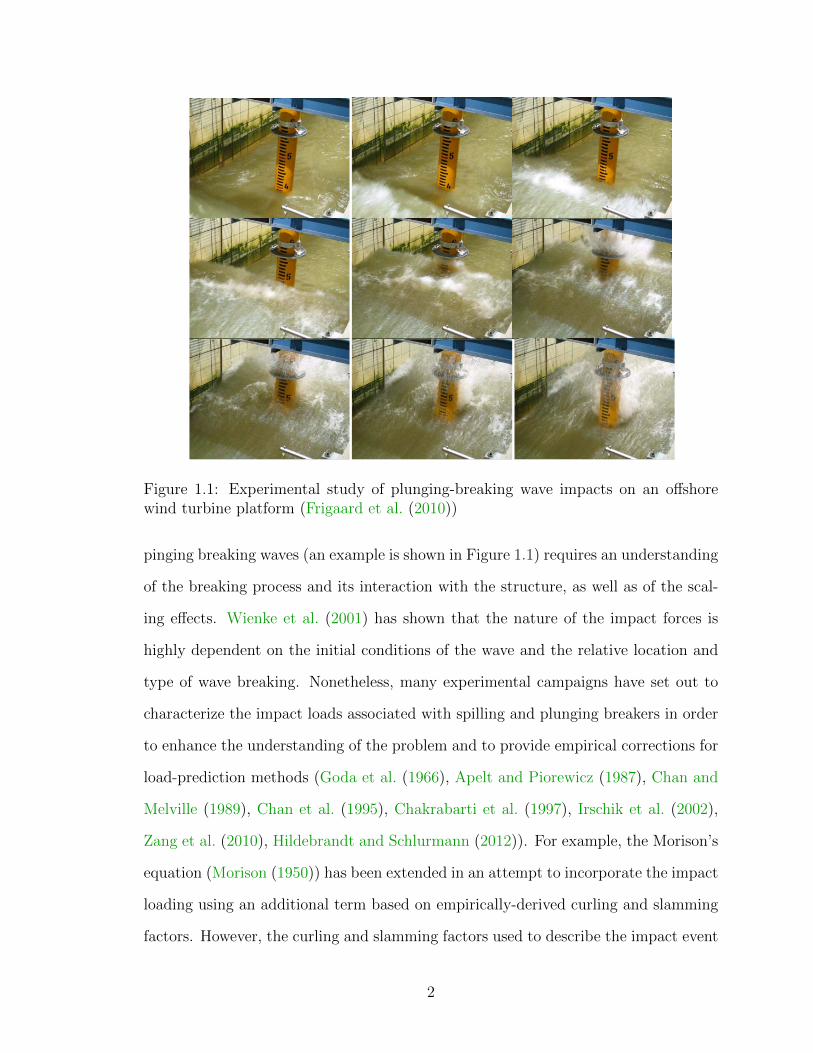
Figure 1.1: Experimental study of plunging-breaking wave impacts on an offshorewind turbine platform (Frigaard et al. (2010))
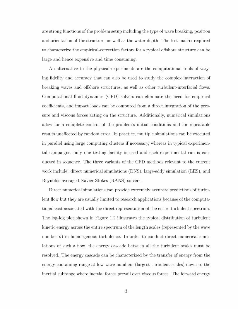
pinging breaking waves (an example is shown in Figure 1.1) requires an understanding
of the breaking process and its interaction with the structure, as well as of the scal-
ing effects. Wienke et al. (2001) has shown that the nature of the impact forces is
highly dependent on the initial conditions of the wave and the relative location and
type of wave breaking. Nonetheless, many experimental campaigns have set out to
characterize the impact loads associated with spilling and plunging breakers in order
to enhance the understanding of the problem and to provide empirical corrections for
load-prediction methods (Goda et al. (1966), Apelt and Piorewicz (1987), Chan and
Melville (1989), Chan et al. (1995), Chakrabarti et al. (1997), Irschik et al. (2002),
Zang et al. (2010), Hildebrandt and Schlurmann (2012)). For example, the Morison’s
equation (Morison (1950)) has been extended in an attempt to incorporate the impact
loading using an additional term based on empirically-derived curling and slamming
factors. However, the curling and slamming factors used to describe the impact event
2
are strong functions of the problem setup including the type of wave breaking, position
and orientation of the structure, as well as the water depth. The test matrix required
to characterize the empirical-correction factors for a typical offshore structure can be
large and hence expensive and time consuming.
An alternative to the physical experiments are the computational tools of vary-
ing fidelity and accuracy that can also be used to study the complex interaction of
breaking waves and offshore structures, as well as other turbulent-interfacial flows.
Computational fluid dynamics (CFD) solvers can eliminate the need for empirical
coefficients, and impact loads can be computed from a direct integration of the pres-
sure and viscous forces acting on the structure. Additionally, numerical simulations
allow for a complete control of the problem’s initial conditions and for repeatable
results unaffected by random error. In practice, multiple simulations can be executed
in parallel using large computing clusters if necessary, whereas in typical experimen-
tal campaigns, only one testing facility is used and each experimental run is con-
ducted in sequence. The three variants of the CFD methods relevant to the current
work include: direct numerical simulations (DNS), large-eddy simulation (LES), and
Reynolds-averaged Navier-Stokes (RANS) solvers.
Direct numerical simulations can provide extremely accurate predictions of turbu-
lent flow but they are usually limited to research applications because of the computa-
tional cost associated with the direct representation of the entire turbulent spectrum.
The log-log plot shown in Figure 1.2 illustrates the typical distribution of turbulent
kinetic energy across the entire spectrum of the length scales (represented by the wave
number k) in homoegenous turbulence. In order to conduct direct numerical simu-
lations of such a flow, the energy cascade between all the turbulent scales must be
resolved. The energy cascade can be characterized by the transfer of energy from the
energy-containing range at low wave numbers (largest turbulent scales) down to the
inertial subrange where inertial forces prevail over viscous forces. The forward energy
3
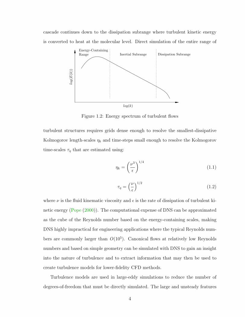
cascade continues down to the dissipation subrange where turbulent kinetic energy
is converted to heat at the molecular level. Direct simulation of the entire range of
Figure 1.2: Energy spectrum of turbulent flows
turbulent structures requires grids dense enough to resolve the smallest-dissipative
Kolmogorov length-scales ηk and time-steps small enough to resolve the Kolmogorov
time-scales τη that are estimated using:
ηk =
(ν3
ε
)1/4
(1.1)
τη =(νε
)1/2
(1.2)
where ν is the fluid kinematic viscosity and ε is the rate of dissipation of turbulent ki-
netic energy (Pope (2000)). The computational expense of DNS can be approximated
as the cube of the Reynolds number based on the energy-containing scales, making
DNS highly impractical for engineering applications where the typical Reynolds num-
bers are commonly larger than O(105). Canonical flows at relatively low Reynolds
numbers and based on simple geometry can be simulated with DNS to gain an insight
into the nature of turbulence and to extract information that may then be used to
create turbulence models for lower-fidelity CFD methods.
Turbulence models are used in large-eddy simulations to reduce the number of
degrees-of-freedom that must be directly simulated. The large and unsteady features
4

of turbulent flow are directly resolved, whereas the smallest scales are separated
(filtered-out) and modeled using so-called subgrid-scale models (Sagaut (2001)). The
large-scale flow features in the energy-containing range are often a function of the
geometry of interest and the smallest turbulent features are assumed to be universal at
sufficiently high Reynolds numbers and hence they should be easier to model. Unlike
the Reynolds-averaged Navier-Stokes approach where the ensemble-averaged mean
flow is computed, large-eddy simulations require relatively dense computational grids
and time-accurate numerical methods to directly represent the large energy-carrying
eddies.
Large-eddy simulations are typically placed between RANS and DNS on the com-
putational expense and accuracy scales (de Villiers (2006)). RANS solvers have been
the main numerical simulation tools for engineering problems due to their relatively
small computational-cost requirements. However, important flow features such as
flow separation, wave breaking, vortex shedding, and turbulence are typically not
resolved accurately or at all. The separation of resolved and modeled scales in LES
theoretically allows for a much improved representation of these important features
that are problem-dependent. Furthermore, the introduction of super-computers and
powerful workstations has allowed for LES and its variants (wall-modeled LES, de-
tached eddy simulations) to become attractive alternatives or complements to the
RANS tools.
In this work, direct numerical simulations and large-eddy simulations are used to
study turbulent-interfacial flows relevant to the marine industry. The DNS data are
used for a priori analysis of the subgrid-scale terms not resolved in LES in order to
understand turbulence in the proximity of a deformable interface. Additionally, the
ability of select turbulence models to account for the subgrid effects in turbulent-
interfacial flows is examined. The a priori analysis is based on two canonical prob-
lems: oil and water phase inversion, and a plunging-breaking wave. The relevant
5
subgrid terms are modeled and assessed a posteriori with large-eddy simulations of
the two canonical problems. The multiphase LES concept is also extended to the
simulation of breaking waves impinging on a vertical circular cylinder to examine the
benefits of high-resolution simulations for industrial problems.
In the following sections, Chapter 2 gives an overview of the literature associated
with numerical simulation of interfacial marine flows with emphasis on breaking-wave
flows. The concept of large-eddy simulations is introduced for single-phase flows and
some of the most common turbulence-closure models are discussed. The LES concept
is then extended to the governing equations of incompressible multiphase flows and the
related literature is summarized. The details of the numerical method are described in
Chapter 3 along with the results of direct numerical simulations of the two canonical
multiphase flows. Chapter 4 presents the a posteriori analysis of the two canonical
problems and of breaking-wave impacts on an offshore structure studied with large-
eddy simulations. Finally, a summary and conclusions are given and possible future
work is proposed in Chapter 5.
6
CHAPTER 2
Background and Related Work
2.1 Simulation of Interfacial Marine Flows
Numerical simulation of turbulent flows with a deformable fluid interface is a complex
problem that is relevant to the marine industry. The interaction of the fluid interface
with turbulence has been studied numerically using several different methodologies
that are typically problem-dependent. In the marine industry, air and water multi-
phase problems are the most common, but the interaction of fuel oil and air as well
as of liquid natural gas (LNG) and air inside of a ship’s storage tanks may also be
of interest. Multiphase flows involving the interaction of air and water are especially
challenging to simulate because the drastic difference of the phase properties can re-
sult in large velocity gradients near the interface and an intricate energy exchange
between the two phases. Additionally, Shen and Yue (2001) have demonstrated that
near-interface turbulent structures are highly anisotropic and can be responsible for
the backscatter of energy that may be on the order of the forward energy cascade
in the proximity of the interface. Breaking-water waves are a common example of a
turbulent-interfacial flow featuring all of the these characteristics.
Early attempts of simulating breaking waves typically involved modeling of the
water phase only. For example, Christensen and Deigaard (2001) describe the free
surface and only the water phase using the surface marker method in order to reduce
7
the computational costs. The simulation of turbulence is based on the large-eddy
simulations approach combined with the traditional Smagorinsky model. Some of
the important features of spilling and plunging-breaking waves such as the near-
interface vortical structures are identified with this approach, but the dissipation of
energy through the air cavity entrainment process and backscatter are unaccounted
for due to the formulation of the numerical method. Watanabe et al. (2005) also study
spilling and plunging breakers using LES of the water phase only and by applying
the kinematic and dynamic boundary conditions at the location of the free surface.
Surface tension effects and air entrainment are not simulated and the authors focus on
the description of the vortical-structures formation process away from the interface.
Several published works focus on the transfer of energy between air and water
during the wave-breaking event. In these types of simulations, the numerical treat-
ment of the interface is commonly based on the Eulerian approach that uses a fixed
grid and a tracking variable assigned to each grid element. Two popular examples
of the Eulerian interface-capturing approach are the volume-of-fluid (VOF) method
and the level-set (LS) method. In VOF, each grid element is assigned a value of the
phase fraction corresponding to the average proportion of each fluid at that location.
The discontinuity of the phase fraction is commonly handled through the simple line
interface calculation (SLIC) or the piecewise-linear interface calculation (PLIC) ap-
proach used to geometrically reconstruction the interface. The level-set method tracks
a signed variable that represents the distance from each cell to the nearest point on
the interface and is positive in one phase and negative in the other phase. Both
methods rely on an additional advection equation that governs the evolution of the
interface. Iafrati (2009) and Iafrati et al. (2012) study two-dimensional water waves
with direct numerical simulations and the level-set interface treatment. The dissipa-
tion of energy through the breaking process is described in detail for both spilling
and plunging breakers in deep water. The early stages of breaking are described well
8
but the three-dimensional turbulent and interfacial structures present in the latter
stages of the flow development cannot be represented on the 2D grids. Zhao et al.
(2004) also use two dimensional domains to study wave breaking using VOF and LES
where the subgrid behavior is modeled with a multi-scale turbulence closure. The au-
thors report a clear separation between the regions of subgrid-scale turbulent kinetic
energy production and dissipation. The lack of local equilibrium during the strong
wave-breaking events can be associated with the backscatter of energy near the inter-
face. Additionally, because eddy-viscosity models are formulated on the basis of such
a local equilibrium, their application to turbulent-interfacial flows is questionable at
best. Two-dimensional waves breaking over a sloping seabed are simulated with LES
by Lubin et al. (2011). The authors acknowledge the need for 3D simulations and a
sufficient level of spatial resolution to correctly describe the energy transfer process
associated with wave breaking. Furthermore, development of a modeling approach to
account for the unresolved-interfacial scales is suggested as an important component
of the future of multiphase large-eddy simulations.
Lubin et al. (2006) examine three-dimensional plunging-breaking waves with large-
eddy simulations and the mixed-scales SGS model. The flow field is initialized with
an artificially-steep linear wave that develops in a computational domain with cycli-
cal boundary conditions. The same concept is used by Iafrati (2009) to reduce the
computational cost of the simulations. The general features of a plunging breaker are
reproduced including the overturning jet and splash-up, and the 3D results indicate
an increase in the energy dissipation rate during the breaking process compared to
the 2D results. Lakehal and Liovic (2011) study the breaking process along a sloping
seabed with LES and a VOF-based method that utilizes a secondary refined grid to
capture the evolution of the interface in greater detail. The information from the
finer grid is used to form a near-interface damping function to correct the overly-
dissipation behavior of the selected eddy-viscosity model. Using spanwise domain
9
averaging, turbulent kinetic energy of a weak plunging-breaking wave is estimated
and found to be not necessarily in equilibrium with the turbulent kinetic energy dis-
sipation. High levels of three-dimensional turbulence are reported in the proximity
of the interface during the breaking process.
Numerical study of wave breaking near the shore is important to the understand-
ing of sediment transport along the coast and simulation of open-ocean wave break-
ing can provide detailed information about the energy exchange process between
the atmosphere and large bodies of water. High-resolution numerical simulation of
turbulent-interfacial flows is also important to the prediction of breaking-wave im-
pacts on offshore structures because of the highly-nonlinear nature of the problem.
de Ridder et al. (2011), Ramirez et al. (2012), and Bredmose et al. (2013) use experi-
mental and numerical analyses to study the response of a bottom-fixed offshore wind
turbine impinged upon by regular and irregular seas that include breaking waves.
A nonlinear potential flow solver is combined with a Morison-based force estimation
in an attempt to numerically replicate the experimental loads on the platform. The
authors report good agreement for relatively small-steepness non-breaking impacts,
whereas the maximum in-line force on the cylindrical platform due to breaking-wave
impacts is significantly under-predicted. The combination of the nonlinear potential
flow and the Morison’s equation cannot sufficiently account for all the phenomena of
plunging breakers that can result in slamming-like impacts. Christensen et al. (2005)
use a volume-of-fluid solver to simulate breaking-wave impacts on a vertical-circular
cylinder. The loads and wave run-up on the structure are found to be strongly influ-
enced by the type and location of wave breaking which are known to be a function of
the air-water interaction. The evolution of the breaking process is further complicated
by the close proximity to the seabed and the turbulent energy exchange between the
two phases that is typically not accounted for in low-order numerical simulations.
The work presented here expands the field of high-resolution simulations of turbulent-
10
interfacial marine flows using direct and large-eddy simulations. The use of high-
resolution methods is important because these methods can describe the complex
interaction between turbulence and the fluid interface in detail and can lead to the
formulation of improved turbulence-closure models. The present analysis evaluates
the turbulence closure terms in the multiphase large-eddy simulations equations that
have been shown to be important in some types of turbulent-interfacial flows. Further-
more, numerical methods readily available for use in complex-industrial large-eddy
simulations are selected in order to allow for a straightforward transfer of the present
findings to practitioners.
2.2 Overview of Large-Eddy Simulations
The separation of scales at the core of the large-eddy simulations concept is formally
achieved through the application of a spatial filter to the governing equations of the
flow. The scales present in the flow are separated into resolved scales and unresolved
or the so-called subgrid scales. The term “subgrid” is used because the concept of
LES is applied on computational domains divided into a matrix (grid) of discrete
computational elements that – unlike DNS grids – cannot fully resolve the entire
range of turbulent scales. The influence of the subgrid scales is represented by the
subgrid-scale (SGS) stress which appears in the filtered momentum equation. This
additional unclosed term can be modeled using several approaches commonly divided
into the functional and structural types.
In the following sections, the filtering concept is first demonstrated for a single-
phase incompressible flow. Different types of interpretation and numerical implemen-
tation of LES are also discussed. Several of the most common subgrid-scale stress
closure models are then described based on Sagaut (2001) who gives a detailed de-
scription of the LES methodology including SGS stress modeling in applications to
11
incompressible flows.
2.2.1 Filtering of the Governing Equations
The low-pass spatial filtering used to obtain the filtered governing equations is defined
as the convolution integral between a filter function G and a generic flow variable φ:
φ(x, t) =
∫G(x− ξ)φ(ξ, t)dξ (2.1)
where the over-bar indicates the filtered or resolved variable and the convolution ker-
nel G is associated with a characteristic cutoff length ∆. The unresolved component
of the generic flow variable is defined as:
φ′ = φ− φ. (2.2)
The three most common filters used in large-eddy simulations are the top-hat or
box filter, the Gaussian filter, and the spectral or sharp cutoff filter. In application
to the Navier-Stokes equations, the selected filter must satisfy linearity, commutation
with derivatives, and the preservation of constants (de Villiers (2006)). In spectral
space (denoted with a hat), the filter kernel is a function of wave number k and the
spatial cutoff length ∆ is associated with a cutoff wave number kc.
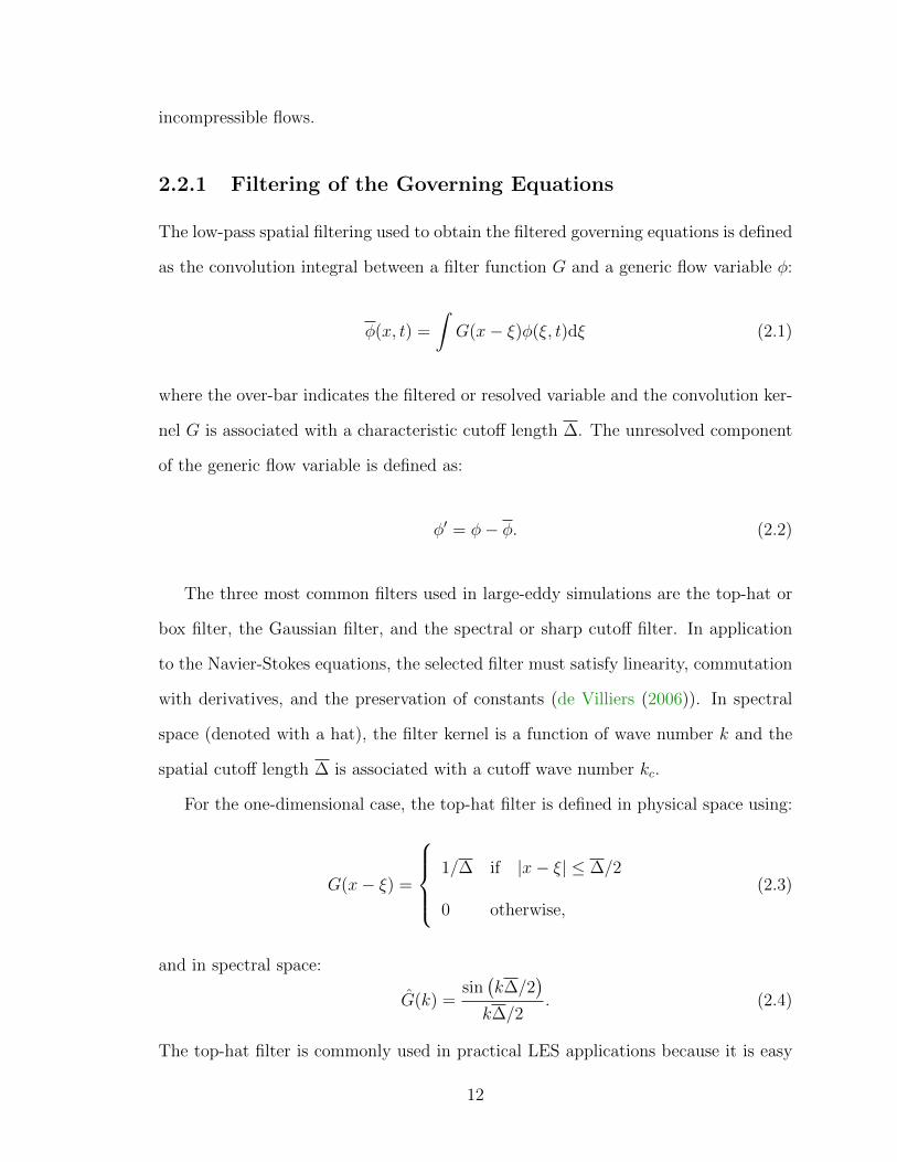
For the one-dimensional case, the top-hat filter is defined in physical space using:
G(x− ξ) =
1/∆ if |x− ξ| ≤ ∆/2
0 otherwise,
(2.3)
and in spectral space:
G(k) =sin(k∆/2
)k∆/2
. (2.4)
The top-hat filter is commonly used in practical LES applications because it is easy
12
to implement numerically and the filter-cutoff length-scale is often taken to be pro-
portional to the grid spacing. Additionally, realistic boundary conditions, such as
solid walls, can be easily used to bound the computational domain because of the
compact support of the filter stencil.
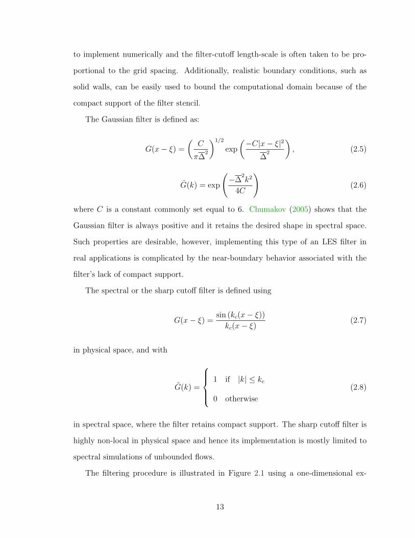
The Gaussian filter is defined as:
G(x− ξ) =
(C
π∆2
)1/2
exp
(−C|x− ξ|2
∆2
), (2.5)
G(k) = exp
(−∆
2k2
4C
)(2.6)
where C is a constant commonly set equal to 6. Chumakov (2005) shows that the
Gaussian filter is always positive and it retains the desired shape in spectral space.
Such properties are desirable, however, implementing this type of an LES filter in
real applications is complicated by the near-boundary behavior associated with the
filter’s lack of compact support.
The spectral or the sharp cutoff filter is defined using
G(x− ξ) =sin (kc(x− ξ))kc(x− ξ)
(2.7)
in physical space, and with
G(k) =
1 if |k| ≤ kc
0 otherwise
(2.8)
in spectral space, where the filter retains compact support. The sharp cutoff filter is
highly non-local in physical space and hence its implementation is mostly limited to
spectral simulations of unbounded flows.
The filtering procedure is illustrated in Figure 2.1 using a one-dimensional ex-
13
-0.5
0
0.5
1
1.5
2
2.5
0 0.2 0.4 0.6 0.8 1
Sig
nal
x
OriginalGrid FilterTest Filter
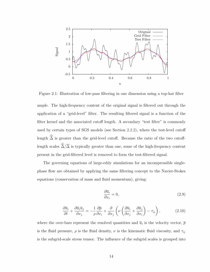
Figure 2.1: Illustration of low-pass filtering in one dimension using a top-hat filter
ample. The high-frequency content of the original signal is filtered out through the
application of a “grid-level” filter. The resulting filtered signal is a function of the
filter kernel and the associated cutoff length. A secondary “test filter” is commonly
used by certain types of SGS models (see Section 2.2.2), where the test-level cutoff
length ∆ is greater than the grid-level cutoff. Because the ratio of the two cutoff-
length scales ∆/∆ is typically greater than one, some of the high-frequency content
present in the grid-filtered level is removed to form the test-filtered signal.
The governing equations of large-eddy simulations for an incompressible single-
phase flow are obtained by applying the same filtering concept to the Navier-Stokes
equations (conservation of mass and fluid momentum), giving:
∂ui∂xi
= 0, (2.9)
∂ui∂t
+∂uiuj∂xj
= −1
ρ
∂p
∂xi+
∂
∂xj
(ν
(∂ui∂xj
+∂uj∂xi
)− τij
), (2.10)
where the over-bars represent the resolved quantities and ui is the velocity vector, p
is the fluid pressure, ρ is the fluid density, ν is the kinematic fluid viscosity, and τij
is the subgrid-scale stress tensor. The influence of the subgrid scales is grouped into
14
τij which is defined as
τij = uiuj − uiuj, (2.11)
based on the decomposition of the nonlinear convective term:
uiuj = uiuj + τij. (2.12)
The SGS stress can be further decomposed using the resolved and subgrid quan-
tities following Germano (1986):
τij = Lij + Cij +Rij, (2.13)
where
Lij = uiuj − uiuj, (2.14)
Cij = uiu′j + uju′i − uiu′j − uju′i, (2.15)
Rij = u′iu′j − u′ju′j (2.16)
are the modified Leonard stress tensor, modified cross-stress tensor, and the modified
Reynolds subgrid tensor, respectively. The modification presented by Germano (1986)
ensures that all three components of the SGS stress are Galilean-invariant. The
Leonard stress represents the interaction of the resolved scales, the cross-stress is
responsible for the interaction between the resolved and the unresolved scales, and the
Reynolds subgrid tensor describes the interaction of the subgrid scales. Certain SGS
models attempt to approximate the indivdual components using information from the
resolved flow (structural type), whereas other types of SGS models approximate the
influence of the entire unclosed term (functional type; see Section 2.2.2 for details of
both modeling approaches).
Several different interpretations and practical implementations of the LES con-
15

cepts can be found in the literature as discussed by Sagaut (2001). The different
methodologies stem from the lack of a consensus on the best-practice guidelines, as
well as from the assumptions and generalizations that are often necessary in practice
to overcome limited computational resources and implementation challenges.
In what is termed the explicit-filtering approach, the filters described above are
applied explicitly on the numerical grid, resulting in the separation of the resolved
scales, subfilter scales, and the subgrid scales. The filter width is selected to be greater
than the grid spacing to allow for an explicit calculation of the filtered quantities based
on the flow information available on the grid level. The scales that cannot be resolved
on the grid due to the limitation of the spatial discretization are represented by the
subgrid-scale stress. This approach is appealing because it can theoretically separate
the influence of the discretization error from the solution approach and because the
explicit application of a filter follows directly from the theoretical formulation of the
LES concept. However, the benefits of explicit LES are unclear in practice. The grid-
level filtering procedure adds an additional computational cost to what are typically
already very expensive computations, and the explicit filtering has been shown to
not guarantee an improvement in the accuracy of the solution. The fully-developed
turbulent channel flow study of Gullbrand and Chow (2003) indicates that a sufficient
grid resolution and an appropriate selection of the SGS model may have a greater
influence on the quality of the solution.
A common alternative to the explicit-filtering approach is referred to as the
implicit-filtering approach, or as the traditional LES solution method in Gullbrand
and Chow (2003). The numerical discretization used to compute the flow solution is
interpreted as an effective low-pass filter and no explicit grid-level filtering is used.
The only filtering that may be applied is used in the calculation of the subgrid-scale
stress model terms such as in the case of a dynamic Smagorinsky model. This method
is commonly found in applications of LES to flows with real-complex geometries and
16
in industrial settings where limited computational resources are available and rapid
turn-around times are necessary. The implicit-filtering method should not be confused
with “no-model” LES or the Monotone Integrated Large-Eddy Simulation (MILES)
in the compressible-flow case where the effective dissipation of high-order upwind
schemes is used exclusively to account for the SGS effects (Fureby (2007)).
In the large-eddy simulations presented in Chapter 4, the implicit-filtering method
is used. Explicit test-level filtering is utilized to model the subgrid-scale behavior
based on the resolved-flow information.
2.2.2 Subgrid-Scale Stress Closure Models
The role of the subgrid-scale stress model is to account for the effects of the unresolved
scales, including the forward and backward energy cascade process. Most models are
categorized as either structural or functional. Structural models (scale-similarity
based) attempt to represent the stress tensor based on the resolved scales, whereas
functional models (eddy-viscosity based) approximate the actual contribution of the
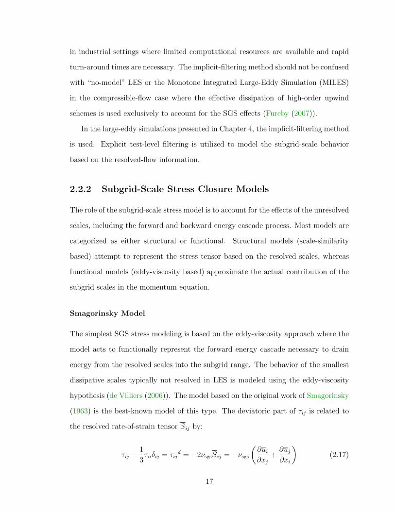
subgrid scales in the momentum equation.
Smagorinsky Model
The simplest SGS stress modeling is based on the eddy-viscosity approach where the
model acts to functionally represent the forward energy cascade necessary to drain
energy from the resolved scales into the subgrid range. The behavior of the smallest
dissipative scales typically not resolved in LES is modeled using the eddy-viscosity
hypothesis (de Villiers (2006)). The model based on the original work of Smagorinsky
(1963) is the best-known model of this type. The deviatoric part of τij is related to
the resolved rate-of-strain tensor Sij by:
τij −1
3τiiδij = τij
d = −2νsgsSij = −νsgs
(∂ui∂xj
+∂uj∂xi
)(2.17)
17
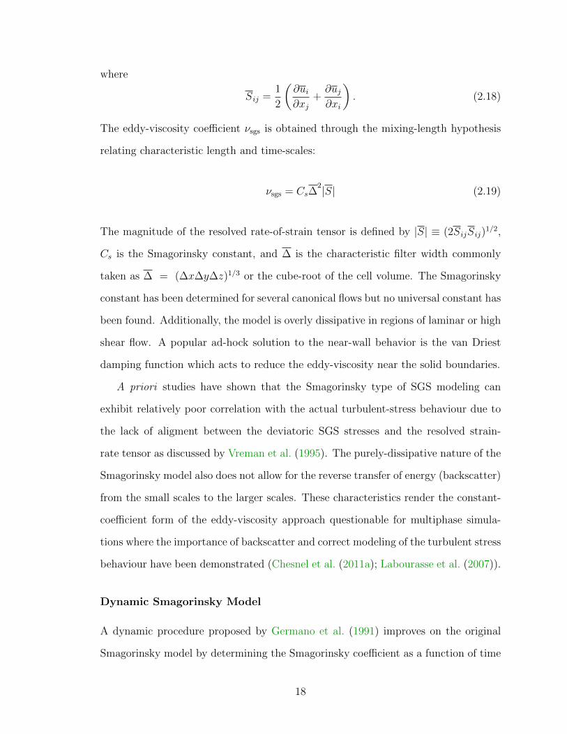
where
Sij =1
2
(∂ui∂xj
+∂uj∂xi
). (2.18)
The eddy-viscosity coefficient νsgs is obtained through the mixing-length hypothesis
relating characteristic length and time-scales:
νsgs = Cs∆2|S| (2.19)
The magnitude of the resolved rate-of-strain tensor is defined by |S| ≡ (2SijSij)1/2,
Cs is the Smagorinsky constant, and ∆ is the characteristic filter width commonly
taken as ∆ = (∆x∆y∆z)1/3 or the cube-root of the cell volume. The Smagorinsky
constant has been determined for several canonical flows but no universal constant has
been found. Additionally, the model is overly dissipative in regions of laminar or high
shear flow. A popular ad-hock solution to the near-wall behavior is the van Driest
damping function which acts to reduce the eddy-viscosity near the solid boundaries.
A priori studies have shown that the Smagorinsky type of SGS modeling can
exhibit relatively poor correlation with the actual turbulent-stress behaviour due to
the lack of aligment between the deviatoric SGS stresses and the resolved strain-
rate tensor as discussed by Vreman et al. (1995). The purely-dissipative nature of the
Smagorinsky model also does not allow for the reverse transfer of energy (backscatter)
from the small scales to the larger scales. These characteristics render the constant-
coefficient form of the eddy-viscosity approach questionable for multiphase simula-
tions where the importance of backscatter and correct modeling of the turbulent stress
behaviour have been demonstrated (Chesnel et al. (2011a); Labourasse et al. (2007)).
Dynamic Smagorinsky Model
A dynamic procedure proposed by Germano et al. (1991) improves on the original
Smagorinsky model by determining the Smagorinsky coefficient as a function of time
18

and space. A secondary test filter, larger than the grid filter and commonly taken
as ∆/∆ = 2, is used to extract information from the resolved scales close to the
grid-filter cutoff. The grid-filtered Navier-Stokes equations are test-filtered (denoted
with the top-hat symbol) to yield a new subtest stress tensor Tij:
Tij = uiuj − uiuj (2.20)
that can be related to the subgrid stress and the resolved stress tensor Lij through
the Germano identity:
Lij = uiuj − uiuj = Tij − τij. (2.21)
Both the subtest and the subgrid stresses can be represented by a general eddy-
viscosity form with the same unknown coefficient Cd:
τij −1
3τkkδij = Cd
(−2∆
2 ∣∣S∣∣Sij) = Cdβij (2.22)
Tij −1
3Tkkδij = Cd
(−2∆
2 ∣∣∣S∣∣∣ Sij) = Cdψij (2.23)
The system is over-determined because there are five independent equations and a
single unknown. A least-squares error minimization was proposed by Lilly (1992) to
find an appropriate eddy-viscosity coefficient where the error Eij is minimized:
Eij = Lij −1
3Lkkδij − Cdψij + Cdβij (2.24)
and the dynamic coefficient is removed from the test-filtering operation in the last
term on the right-hand side through the assumption of Cd being constant over an
interval on the order of the test filter length. The coefficient is then obtained from:
Cd =mijL
dij
mklmkl
(2.25)
19
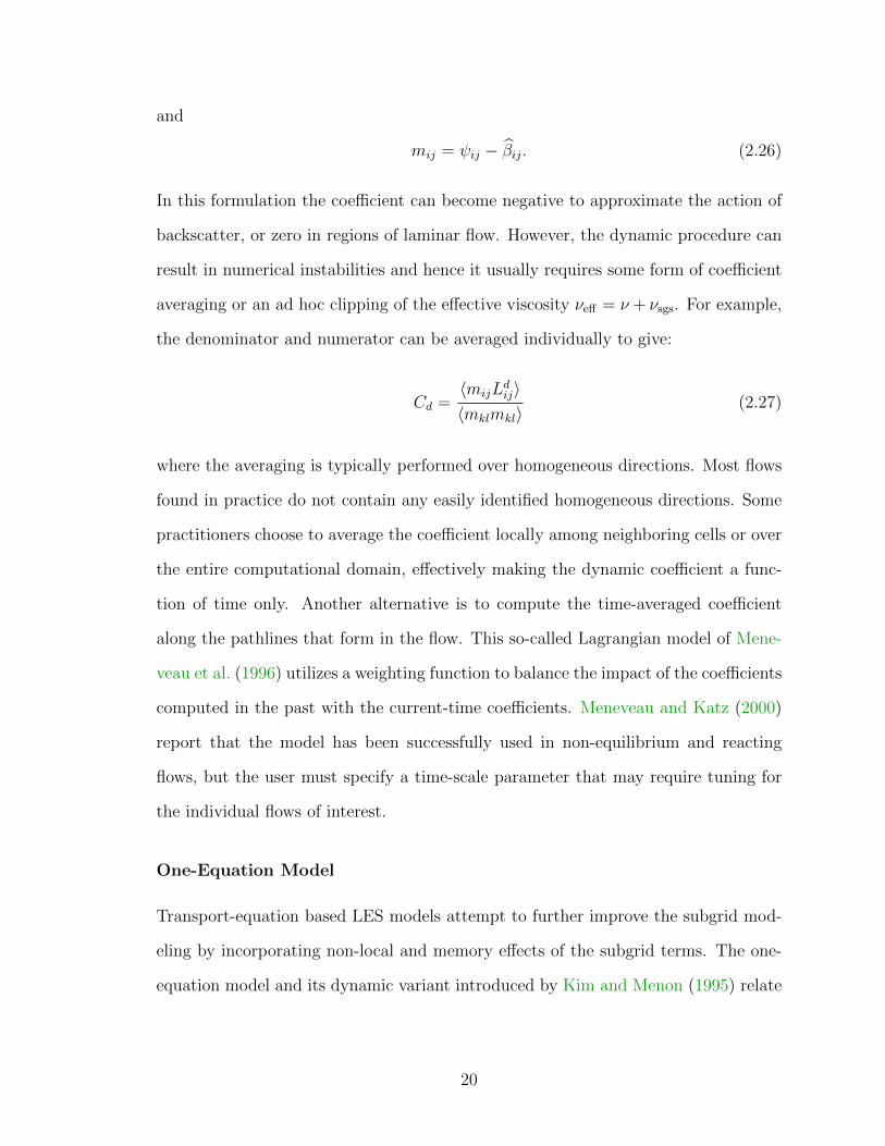
and
mij = ψij − βij. (2.26)
In this formulation the coefficient can become negative to approximate the action of
backscatter, or zero in regions of laminar flow. However, the dynamic procedure can
result in numerical instabilities and hence it usually requires some form of coefficient
averaging or an ad hoc clipping of the effective viscosity νeff = ν + νsgs. For example,
the denominator and numerator can be averaged individually to give:
Cd =〈mijL
dij〉
〈mklmkl〉(2.27)
where the averaging is typically performed over homogeneous directions. Most flows
found in practice do not contain any easily identified homogeneous directions. Some
practitioners choose to average the coefficient locally among neighboring cells or over
the entire computational domain, effectively making the dynamic coefficient a func-
tion of time only. Another alternative is to compute the time-averaged coefficient
along the pathlines that form in the flow. This so-called Lagrangian model of Mene-
veau et al. (1996) utilizes a weighting function to balance the impact of the coefficients
computed in the past with the current-time coefficients. Meneveau and Katz (2000)
report that the model has been successfully used in non-equilibrium and reacting
flows, but the user must specify a time-scale parameter that may require tuning for
the individual flows of interest.
One-Equation Model
Transport-equation based LES models attempt to further improve the subgrid mod-
eling by incorporating non-local and memory effects of the subgrid terms. The one-
equation model and its dynamic variant introduced by Kim and Menon (1995) relate
20

the turbulent viscosity to the subgrid turbulent kinetic energy by:
νsgs = Ck∆k1/2sgs . (2.28)
A transport equation for ksgs is constructed and takes the form:
∂ksgs
∂t+∂ujksgs
∂xj= −τij
∂ui∂xj− Cε
k3/2sgs
∆+
∂
∂xj
(νsgs
∂ksgs
∂xj
)(2.29)
where the first term on the right-hand side is the production term. The dissipa-
tion term follows and its coefficient Cε together with Ck can be determined dynami-
cally based on the Germano identity previously discussed in the case of the dynamic
Smagorinsky model (Equation 2.21). An approximation of backscatter is possible
without the numerical stability issues often found in the original Smagorinsky models
because of the implemented limiting mechanisms (Carati et al. (1995)). The addi-
tional transport-equation and the dynamic procedure required to compute the model’s
coefficients make this form of LES modeling more computationally expensive. Carati
et al. (1995) has shown that the dynamic one-equation model requires approximately
70% more computational overhead than the original constant-coefficient Smagorinsky
model for simulations of isotropic turbulence decay and forced turbulence.
Scale-Similarity Models
Bardina et al. (1980) proposed the scale-similarity model in which the modeled subgrid
terms are computed from the smallest resolved scales. This form of structural LES
turbulence modeling is based on the conjecture that the SGS stresses are correlated
with the Reynolds stresses due to the smallest resolved scales (Sarghini et al. (1999)).
A secondary grid-level filtering operation is performed to obtain the subgrid stress
term of the form:
τij = uiuj − uiuj (2.30)
21
which corresponds to the modified Leonard stress and is expressed in terms of the
resolved quantities only. A priori studies of Bardina et al. (1980) and others have
shown excellent correlation between the similarity-modeled SGS stress and the true
SGS stress computed from DNS data of homoegenous isotropic turbulence and shear
turbulent flows. The backscatter of energy is accounted for in a stable manner using
this formulation but because the pure scale-similarity model is not dissipative in
nature, it is often found to lack sufficient dissipation in the subgrid regime (Zang
et al. (1993)).
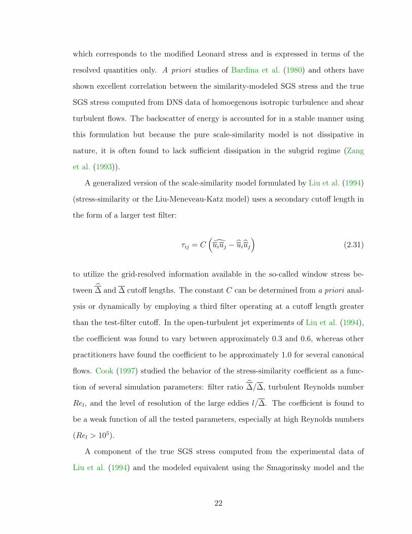
A generalized version of the scale-similarity model formulated by Liu et al. (1994)
(stress-similarity or the Liu-Meneveau-Katz model) uses a secondary cutoff length in
the form of a larger test filter:
τij = C(uiuj − uiuj
)(2.31)
to utilize the grid-resolved information available in the so-called window stress be-
tween ∆ and ∆ cutoff lengths. The constant C can be determined from a priori anal-
ysis or dynamically by employing a third filter operating at a cutoff length greater
than the test-filter cutoff. In the open-turbulent jet experiments of Liu et al. (1994),
the coefficient was found to vary between approximately 0.3 and 0.6, whereas other
practitioners have found the coefficient to be approximately 1.0 for several canonical
flows. Cook (1997) studied the behavior of the stress-similarity coefficient as a func-
tion of several simulation parameters: filter ratio ∆/∆, turbulent Reynolds number
Rel, and the level of resolution of the large eddies l/∆. The coefficient is found to
be a weak function of all the tested parameters, especially at high Reynolds numbers
(Rel > 105).
A component of the true SGS stress computed from the experimental data of
Liu et al. (1994) and the modeled equivalent using the Smagorinsky model and the
22
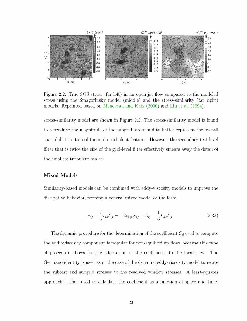
Figure 2.2: True SGS stress (far left) in an open-jet flow compared to the modeledstress using the Smagorinsky model (middle) and the stress-similarity (far right)models. Reprinted based on Meneveau and Katz (2000) and Liu et al. (1994).
stress-similarity model are shown in Figure 2.2. The stress-similarity model is found
to reproduce the magnitude of the subgrid stress and to better represent the overall
spatial distribution of the main turbulent features. However, the secondary test-level
filter that is twice the size of the grid-level filter effectively smears away the detail of
the smallest turbulent scales.
Mixed Models
Similarity-based models can be combined with eddy-viscosity models to improve the
dissipative behavior, forming a general mixed model of the form:
τij −1
3τkkδij = −2νsgsSij + Lij −
1
3Lkkδij. (2.32)
The dynamic procedure for the determination of the coefficient Cd used to compute
the eddy-viscosity component is popular for non-equilibrium flows because this type
of procedure allows for the adaptation of the coefficients to the local flow. The
Germano identity is used as in the case of the dynamic eddy-viscosity model to relate
the subtest and subgrid stresses to the resolved window stresses. A least-squares
approach is then used to calculate the coefficient as a function of space and time.
23
Additionally, a third filter-cutoff length-scale can be utilized to dynamically compute
the coefficient for the similarity contribution, resulting in the so-called dynamic two
parameter model of Salvetti and Banerjee (1995).
Mixed models have been found to improve on the correlation between the mod-
eled SGS stresses and the true SGS stresses compared to the original Smagorinsky
model because the eddy-viscosity contribution is typically much smaller compared to
the scale-similarity term. A priori testing of DNS data for spray atomization flows
by Chesnel et al. (2011a) showed a significant improvement in the correlation coeffi-
cient between the modeled and true SGS stresses and the author also acknowledged
the mixed model as the most promising approach to future multiphase large-eddy
simulations.
Evaluating Model Performance
Two methods of SGS model evaluation are commonly used in practice: a priori
and a posteriori studies. In the a priori analysis, direct numerical simulations or
experimental measurements are used as the exact solution to the flow of interest.
Because the experimental data set is a direct representation of the real flow and the
DNS data is considered to be fully resolved across all the scales of turbulence, the
resolved and subgrid quantities are computed freely. Liu et al. (1994) outlines the
a priori procedure conducted for experimental measurements of an open jet at a
relatively high Reynolds number. The consistency of the procedure is emphasized
to ensure that when computing the flow quantities for the analysis of the large-eddy
simulations models, only the information available at the LES grid level is used. This
entails explicit filtering of the experimental data and sampling it onto the effective
LES grid that is coarser than the spatial resolution of the experiments. The true
subgrid-scale stress can then be compared to the modeled stress at the locations of the
LES grid points without the influence of additional information that is not available
24

during the execution of large-eddy simulations. The same procedure has been applied
to a priori studies of various flows resolved with direct numerical simulations (see for
example Vreman et al. (1995), Chesnel et al. (2011a)).
The a priori analysis is useful for a direct comparison of the true SGS stress and
the modeled SGS stress, but because the flow quantities that are used originate from
either DNS or experiments, the effects of numerical error that is inherent to LES
solutions is not taken into account. The a posteriori method includes the numerical
error effects into the evaluation of the SGS models by comparing the results of actual
large-eddy simulations against reference data. The difficulty of this method stems
from a large number of factors that may affect the LES results and that may be
beyond the control of the practitioner. The approach used in this work is to use both
the a priori (Chapter 3) and the a posteriori (Chapter 4) analyses to study the nature
of the subgrid terms and to evaluate the subgrid-scale models of interest based on
two canonical turbulent-interfacial flows.
2.3 Large-Eddy Simulations of Interfacial Flows
The filtering concept is now extended to the governing equations of multiphase flow.
Two incompressible and immiscible fluids separated by a deformable interface can
be simulated numerically based on the formulation of Scardovelli and Zaleski (1999).
In this so-called one-fluid formulation, a single set of governing equations (here also
referred to as the multiphase equations) describes the entire computational domain
and the behavior of the fluid interface is captured by an additional equation. The
governing equations are filtered and the relative magnitudes of the resulting subgrid-
scale stresses are discussed based on published a priori studies of relavent turbulent-
interfacial flows.
25

2.3.1 Governing Equations
The general form of the multiphase equations including gravitational and viscous
forces can be formulated as:
∂ui∂xi
= 0 (2.33)
∂ρui∂t
+∂ρuiuj∂xj
= − ∂p
∂xi+ ρgi +
∂
∂xj
(µ
(∂ui∂xj
+∂uj∂xi
))− S(xi, t). (2.34)
The equations include the conservation of mass and momentum with a generic source
term S(xi, t). The general form of the interface equation for interface-capturing meth-
ods applied to incompressible flows can be formulated as:
∂α
∂t+∂uiα
∂xi= 0. (2.35)
The fluid properties are defined everywhere in the domain using the phase-indicator
variable α that is represented by the volume fraction in the volume-of-fluid (VOF)
method and the regularized characteristic function in the conservative level-set (CLS)
method that is adapted in this work. The fluid density and viscosity is defined
everywhere in the domain using:
ρ(xi) = ρwα(xi) + ρa (1− α(xi)) , (2.36)
µ(xi) = µwα(xi) + µa (1− α(xi)) . (2.37)
In simulations of air and water, α = 0 corresponds to a computational cell occupied by
air and α = 1 indicates a computational cell occupied by water. The interface between
the two fluids is a thin smoothly-varying region referred to as the diffuse interface and
the nominal free surface is found where α = 0.5. The continuum surface force (CSF)
model of Brackbill et al. (1992) is adapted in the present work to include the effects
of surface tension. A continuous volumetric force is introduced into the momentum
26
equation to model surface tension acting within the diffuse interface (Rusche (2002)).
Following the single-phase derivation presented in Section 2.2.1, the generalized
governing equations are filtered to yield:
∂ui∂xi
= 0, (2.38)
∂ρui∂t
+∂ρuiuj∂xj
= − ∂p
∂xi+ ρgi +
∂
∂xj
(µ
(∂ui∂xj
+∂uj∂xi
))− γκ ∂α
∂xi(2.39)
for the conservation of fluid mass and momentum in the one-fluid formulation. The
last term of the right-hand side of Equation 2.39 is the continuum surface force model
for surface tension where γ is the surface tension coefficient, and κ is the surface
curvature. The interface-advection equation is also filtered resulting in:
∂α
∂t+∂uiα
∂xi= 0. (2.40)
The low-pass filtering operation commutes with the derivative operator and constants
that are not a function of the spatial coordinates are unaffected. The nonlinear terms
that depend on the unresolved scales are decomposed using the generalized form of
Equation 2.12 to give the following set of governing equations:
∂ui∂xi
= 0 (2.41)
∂ρ ui∂t
+∂ρ uiuj∂xj
= − ∂p
∂xi+ρgi+
∂
∂xj
(µ
(∂ui∂xj
+∂uj∂xi
))− ∂τAi
∂t− ∂τCij
∂xj− ∂τDij
∂xj−τST i
(2.42)
∂α
∂t+∂uiα
∂xi= −∂τI i
∂xi(2.43)
The influence of the unresolved scales is grouped into four subgrid-scale terms in the
27

filtered momentum equation and into one SGS term in the filtered interface equation:
τAi = ρui − ρ ui (2.44)
τCij = ρuiuj − ρ uiuj (2.45)
τDij = µ
(∂ui∂xi
+∂uj∂xi
)− µ
(∂ui∂xj
+∂uj∂xi
)(2.46)
τST i = γκ∂α
∂xi(2.47)
τI i = uiα− uiα (2.48)
The five terms are referred to as the acceleration, convective, diffusive, surface tension,
and interfacial subgrid-scale terms, respectively. The convective term is found in the
single-phase LES equations, whereas the other terms are related to the presence of
the fluid interface (Labourasse et al. (2007), Chesnel et al. (2011a)).
The application of the spatial filter across the finite thickness of the interface
has the side-effect of introducing the new subgrid terms in the single-fluid equations.
The effects of the additional subgrid terms are a function of the interface thickness.
In order to avoid filtering across the interface, the filter size must diminish in the
interface region, or in the case of the implicit filtering, the grid size near the interface
must be infinitesimally small. However, because the approximation of the interface
using the diffuse-interface approach and implicit filtering are common in engineering
applications, it is important to understand the impact of the additional terms using
grid refinement levels that are used in practice.
In applications to compressible flow, the Navier-Stokes equations are commonly
Favre-averaged to reduce the number of subgrid terms in the filtered equations. The
28

Favre-averaged generic flow variable is obtained from:
φ =ρφ
ρ. (2.49)
The correlation between the variable-fluid density ρ and the flow variable φ is removed
using the Favre-average and hence the acceleration SGS term τA is eliminated. In the
present work, the Favre-average is not used because when both phases are incompress-
ible the application of the Favre operation yields a source term in the conservation
of mass equation (see Toutant et al. (2009), Chesnel et al. (2011a), Labourasse et al.
(2007) for details). The additional source term is not trivial to handle numerically
and the added difficulty of its implementation at least partially outweighs the benefits
of reducing the number of SGS terms. Additionally, as will be shown in the a priori
study of Chapter 3, the acceleration term that is eliminated by the Favre-average is
found to be several orders of magnitude smaller than the other SGS terms for the
two flows studied.
2.3.2 Role of Subgrid Scales
Several recently published works have investigated the subgrid-scale terms present in
the multiphase LES equations. Lakehal and Liovic (2011) note that the choice to
either model or neglect the SGS terms should be made based on a thorough study
of their relative importance. Such studies have been conducted for relatively simple
turbulent-interfacial flows to allow for the use of direct numerical simulations and
the a priori analysis. The magnitudes of the SGS terms are quantified using the
filtered DNS data and compared to the resolved terms to determine the amount of
information that would typically be not resolved through large-eddy simulations of
the same flows.
The problem of oil-water phase inversion in a closed box is examined by Labourasse
29
et al. (2007), Vincent et al. (2008), and Larocque et al. (2010). The same flow is also
studied in the present work. Labourasse et al. (2007) use a two-dimensional 5122
cell grid together with the piecewise-linear interface calculation (VOF-PLIC) method
and hybrid center-upwind discretization schemes. The a priori analysis uses a top-
hat filter with four different stencil sizes. A comparison is also made between the
results obtained with and without Favre-averaging of the governing equations. The
authors report that the subgrid behavior of the flow cannot be fully represented with
modeling of the convective term only. The convective term is found to be the largest
contributor relative to the resolved quantities, but the magnitudes of the diffusive and
surface-tension SGS terms change rapidly as the filter size is modified. The Favre-
filtered version of the governing equations is recommended for use in LES because the
results with this approach were found to be less diffusive and hence possibly easier to
correct for with the addition of eddy-viscosity models. However, the implementation
of the source term in the continuity equation that is due to Favre-averaging is not
taken into account. The benefits of the mixed model for the convective term are also
reported in comparison to pure eddy-viscosity models.
Vincent et al. (2008) and Larocque et al. (2010) study the phase inversion problem
using three-dimensional grids with 1283 elements and two sizes of the top-hat filter.
Favre-averaging is used in both works to eliminate the acceleration SGS term. The
relative magnitude of the remaining SGS terms is examined as a function of the fluid
density and viscosity ratios. The Reynolds number in water is varied between 1×10⁴
and 5.54 × 10⁵, and the Weber number is varied between 26 and 1.3 × 10⁴. In this
parametric study, Larocque et al. (2010) find the magnitude of the convective SGS
term to be approximately 25% of the resolved counterpart. The subgrid interfacial
term τI is found to be on the order of the resolved component, and the authors state
that τC and τI should be the focus of SGS modeling in large-eddy simulations of
similar turbulent-interfacial flows. The relative order of the SGS term contributions
30

is unaffected by the adjustment of the non-dimensional flow parameters.
Chesnel et al. (2011a) conduct direct numerical simulations of spray atomization
to study the hierarchy of the subgrid terms present in the multiphase formulation.
The simulations are conducted on a grid with approximately 134 million cells and
the ghost fluid method is coupled with a VOF/LS approach to preserve the sharp
fluid interface. A priori analysis indicates that the evolution of the fluid interface is
heavily influenced by the subgrid behavior. The stress-similarity model was found to
exhibit an excellent correlation between the true and modeled subgrid interfacial con-
tribution. However, the coefficient of the model was adjusted based on the filter-size
ratio using the DNS results. A procedure for calculating the coefficient dynamically is
indicated as the optimal solution for the application of the stress-similarity model in
practical multiphase LES. The authors report that the convective SGS stress cannot
be successfully modeled with a pure eddy-viscosity concept when a fluid interface is
present. The poor performance of the eddy-viscosity model is associated with the for-
mation of strong velocity gradients caused by the presence of the interface rather than
turbulent motion. The mixed modeling concept shows a much improved correlation
with the true SGS stress compared to the dynamic Smagorinsky model.
The current work utilizes similar analyses based on highly-resolved numerical sim-
ulations to study the subgrid behavior in turbulent-interfacial flows relevant to the
marine industry. A priori analysis of the LES subgrid-scale terms is carried out to de-
termine their relative importance in incompressible multiphase flows using DNS data
for two canonical problems: oil and water phase inversion, and a plunging-breaking
wave. The performance of select turbulence models in multiphase applications in-
volving a deformable interface is examined using the DNS data. The relevant subgrid
terms are then modeled and assessed a posteriori with large-eddy simulations of the
two canonical problems. The additional subgrid terms are modeled with the stress-
similarity concept that is implemented into the LES solver. Additionally, the multi-
31

phase large-eddy simulations concept is extended to an industrial problem involving
breaking waves impinging on a vertical circular cylinder. The effects of the subgrid
modeling on the ability to predict the force on the cylinder and the free-surface ele-
vation profiles are investigated, and the contributions of the subgrid terms due to the
presence of the interface are examined.
32
CHAPTER 3
Direct Numerical Simulations of
Canonical Interfacial Flows
In this chapter, highly-resolved numerical simulations are used to study two types of
turbulent-interfacial flows. The generated data is used for a priori analysis of the
various subgrid-scale terms present in the grid-filtered governing equations, and for
the analysis of several commonly used subgrid-scale modeling approaches.
First, the problem of two fluids interacting inside of a closed two-dimensional
domain is examined. This phase-inversion problem involves a complex interaction of
a wide range of turbulent and interfacial scales that are resolved on a fine numerical
grid. The turbulent and interfacial structures present in this canonical flow are of
interest because they are directly related to the types of turbulent and interfacial
structures found in marine flows with breaking waves. The problem setup allows
for the use of a trivial domain geometry, high-accuracy uniform numerical grids and
discretization schemes. The second canonical flow study involves a three-dimensional
plunging-breaking wave. Uniform grids and high-accuracy discretization schemes are
also used here to simulate the breaking process of a steep water wave.
An overview of the numerical method employed in this work is presented first.
The sections that follow introduce the two canonical flows and present the details
of grid convergence studies that are conducted to ensure an adequate resolution of
the turbulent and interfacial scales of interest. The subgrid-scale terms identified in
33
Chapter 2 are then quantified and examined for their relative importance. The results
of the two a priori studies are used in Chapter 4 to carry out large-eddy simulations
of the two turbulent-interfacial flows.
3.1 Numerical Method
The numerical simulations performed in this work utilize the OpenFOAM open-source
toolkit that consists of a large set of numerical solvers and discretization schemes
commonly used to numerically solve partial differential equations that govern fluid
flow. The standard set of C++ libraries can be easily modified and extended to
include new turbulence models, treatments of the fluid interface, solution algorithms,
etc. The capabilities of OpenFOAM to simulate single and multiphase flows have
been studied and validated by a large community of developers, researchers, and
practitioners across many industries.
The computational domain is decomposed into a set of control volumes (compu-
tational cells) and the governing equations are discretized based on the finite-volume
method (FVM, see Ferziger and Peric (1996) for details). Because the OpenFOAM
toolkit is three-dimensional in nature, two-dimensional grids are one-cell thick and
use special boundary conditions to eliminate the influence of the third dimension.
The governing equations of the fluid flow, such as those presented in Sections 2.2.1
and 2.3.1, contain spatial terms that are discretized based on the generalized form of
Gauss’ theorem (see for example Damian (2012)). The temporal terms of the govern-
ing equations can be handled with explicit or implicit methods. The flow variables
are stored at the cell centers in a co-located arrangement and the system of equations
is solved in a segregated approach. Jasak (1996) provides a detailed description of
the general discretization and solution methodology.
34
3.1.1 Solution Procedure
The solution to the discretized incompressible Navier-Stokes equations is computed
using the classical PISO (Pressure Implicit with Splitting of Operators) algorithm
where the momentum predictor and corrector steps handle the pressure-velocity cou-
pling (Issa (1986)). The fluid-interface equation is solved with the conservative level-
set method (CLS) of Olsson and Kreiss (2005) and Olsson et al. (2007). In this
method, the mass-conserving properties of the volume-of-fluid formulation are com-
bined with the benefits of the level-set approach including the smooth transition of
the fluid properties across the interface region of constant width. The regularized
characteristic function α varies from 0 to 1 across the interface thickness defined by
the hyperbolic tangent function and the nominal interface is defined where α = 0.5.
The process of advecting the characteristic function is completed in two steps that
involve solving a set of partial differential equations:
∂α
∂t+∂uiα
∂xi= 0, (3.1)
∂α
∂τ+
∂
∂xi(α (1− α)ni) = ε
∂
∂xi
((∂αni∂xi
)ni
). (3.2)
The first equation corresponds to the interface-advection equation presented in Sec-
tion 2.3.1. The steady-state solution of Equation 3.2 is obtained between each time
step to preserve the desired interface thickness and is referred to as the reinitialization
step. The constant ε is proportional to the thickness of the diffuse interface and its
value is selected at run-time. The vector normal to the fluid interface ni is found
using:
ni =∂α
∂xi
∣∣∣∣ ∂α∂xi∣∣∣∣−1
. (3.3)
The CLS method has been validated for both convergence and mass-conservation
properties using several canonical interfacial-flow problems including falling droplets,
35

raising air bubbles, vortex and rotating circle tests.
The two flows studied in this chapter use simple domain geometries that are
discretized using uniformly-spaced hexahedral cells with an aspect ratio of one. The
quality of these grids allows for the use of second-order accurate central-difference
schemes to discretize the spatial terms in the governing equations. The geometry
used in last case study of Chapter 4 is far-more complex because it involves a sloping
seabed and a vertical-circular cylinder piercing the air-water interface. Because cell
stretching and relatively large cell aspect ratios are necessarily used in this case, flux-
limited schemes are used to discretize the convective terms in both the momentum
equation and the interface equation to preserve the monotonicity of the solution while
retaining an overall second-order accuracy (Jasak (1996)). The temporal derivatives
are discretized using backward differencing that utilizes two old time levels to achieve
second-order accuracy. The pressure equation is solved with a generalized geometric-
algebraic multi-grid (GAMG) solver and the other linear systems are solved with the
preconditioned bi-conjugate gradient (PBiCG) solver.
3.1.2 Filtering Operation
The explicit filters applied in both the a priori and a posteriori studies are based
on the top-hat filter discussed in Section 2.2.1. The filter stencil is discretized based
on the work of Chesnel et al. (2011a), Larocque et al. (2010), Toutant et al. (2009),
Vincent et al. (2008), and Labourasse et al. (2007) where an effective volume-average
of the sampled neighboring cells is computed at each cell center using:
φ(i, j, k) =1
(2N + 1)3
N∑n=−N
N∑m=−N
N∑l=−N
φ(i+ n, j +m, k + l) (3.4)
with 2N + 1 = ∆/∆, and ∆ is the LES grid-level cutoff length and ∆ is the DNS
grid spacing. In the a priori analysis, the filtered data is then down-selected onto an
36
effective LES grid that is coarser than the DNS resolution and is a function of the
∆/∆ ratio. This process ensures that only the information that would be available
during actual large-eddy simulations is used to compute the modeled subgrid-scale
terms and that the correlation between the modeled and true subgrid terms is not
artificially enhanced by the use of information only accessible at the DNS level.
3.1.3 Validation of the A Priori Procedure
The a priori procedure is validated using the classical DNS and LES benchmark-
ing study of the fully-developed turbulent channel flow. Several components of the
subgrid-scale stress τij are calculated using DNS data and compared to the results of
Salvetti and Banerjee (1995). Additionally, the implementation of the coefficient cal-
culation procedure used by dynamic SGS models is verified by comparing the spatial
distribution of Cd inside of the channel against the previously-published results. The
consistency of the a priori procedure is ensured by following the detailed description
of Liu et al. (1994).
Salvetti and Banerjee (1995) calculate the SGS stresses using direct numerical
simulations of a modified channel flow problem characterized by a no-slip wall and a
free-slip boundary. The Reynolds number based on the shear velocity at the no-slip
wall is Reτ = 171. The same problem setup is reproduced in OpenFOAM using
second-order schemes that are demonstrated by van Haren (2011) to be fully capable
of reproducing high-accuracy DNS results of canonical flows. The computational
grid consists of uniformly spaced cells in the streamwise and spanwise directions and
of nonuniform grid spacing in the wall-normal direction. The small cells near the
no-slip boundary allow for a detailed resolution of the viscous sublayer. The RMS
velocity fluctuations and the mean velocity profile are compared against the published
DNS data to ensure that the solution is converged. Additionally, the classical fully-
developed turbulent channel flow at Reτ = 180 with two no-slip walls is also validated
37

against the results of Kim et al. (1987) to verify an adequate resolution of the smallest
scales of turbulence with the current numerical method.
0
1
2
3
4
5
0 20 40 60 80 100 120 140 160
τ 11
z+
PresentSalvetti and Banerjee (1995)
(a) SGS Stress: τ11
-0.6
-0.5
-0.4
-0.3
-0.2
-0.1
0
0 20 40 60 80 100 120 140 160
τ 13
z+
PresentSalvetti and Banerjee (1995)
(b) SGS Stress: τ13
Figure 3.1: Subgrid-scale stress components for the fully-developed turbulent channelflow (Reτ = 171)
Two components of the subgrid-scale stress (τ11 and τ13) are shown in Figure 3.1(a)
and Figure 3.1(b) as a function of non-dimensional distance to the wall z+. The stress
components are averaged on the homogeneous-horizontal planes parallel to the wall
boundary. The component subscripts (1,2,3) correspond to the streamwise, spanwise,
and normal directions, respectively. The general trends of the two subgrid stress
components agree well with the reference results. Both stresses approach zero close
to the no-slip boundary at z+ = 0 and towards the middle of the channel approaching
z+ = 160. The location of the peak values of both components is predicted correctly,
but the magnitudes are somewhat different compared to the reference results. Unlike
the DNS method used here, the DNS data used by Salvetti and Banerjee (1995) were
38
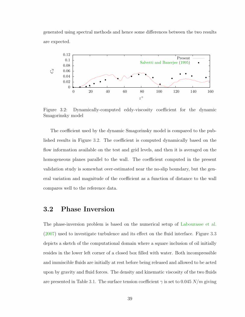
generated using spectral methods and hence some differences between the two results
are expected.
0
0.02
0.04
0.06
0.08
0.1
0.12
0 20 40 60 80 100 120 140 160
Cd
z+
PresentSalvetti and Banerjee (1995)
Figure 3.2: Dynamically-computed eddy-viscosity coefficient for the dynamicSmagorinsky model
The coefficient used by the dynamic Smagorinsky model is compared to the pub-
lished results in Figure 3.2. The coefficient is computed dynamically based on the
flow information available on the test and grid levels, and then it is averaged on the
homogeneous planes parallel to the wall. The coefficient computed in the present
validation study is somewhat over-estimated near the no-slip boundary, but the gen-
eral variation and magnitude of the coefficient as a function of distance to the wall
compares well to the reference data.
3.2 Phase Inversion
The phase-inversion problem is based on the numerical setup of Labourasse et al.
(2007) used to investigate turbulence and its effect on the fluid interface. Figure 3.3
depicts a sketch of the computational domain where a square inclusion of oil initially
resides in the lower left corner of a closed box filled with water. Both incompressible
and immiscible fluids are initially at rest before being released and allowed to be acted
upon by gravity and fluid forces. The density and kinematic viscosity of the two fluids
are presented in Table 3.1. The surface tension coefficient γ is set to 0.045 N/m giving
39

Figure 3.3: Sketch of the computational domain with the main parameters for thephase-inversion problem
a Weber number of We = 1, 090 defined as:
We =(ρw − ρo)u0
2L/2
γ. (3.5)
A references velocity is obtained from u0 =√gL where g is the gravitational accel-
eration and L is the width and height of the computational domain. The Reynolds
number based on u0, the height of the oil inclusion L/2, and the corresponding fluid
density and viscosity is computed as:
Reo,w =ρo,wu0L/2
µo,w(3.6)
to give Rew = 99, 000 in water and Reo = 1, 456 in oil. No-slip boundary conditions
are applied at all four walls bounding the domain.
Several grid resolutions are tested to ensure solution convergence with grid re-
finement and a sufficient resolution of the turbulent scales. The details of the grids,
including the spatial and temporal resolution, are included in Table 3.2. The pre-
viously published DNS studies of the same phase-inversion problem used uniform
40
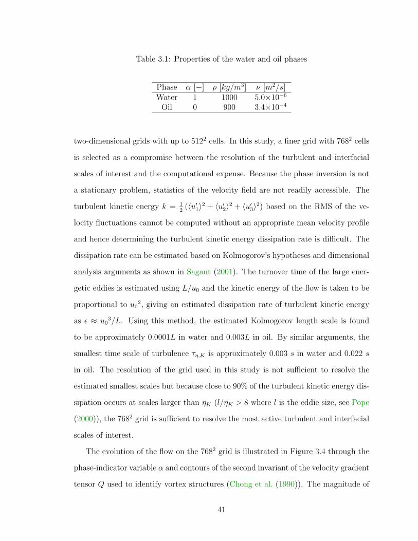
Table 3.1: Properties of the water and oil phases
Phase α [−] ρ [kg/m3] ν [m2/s]Water 1 1000 5.0×10⁻⁶
Oil 0 900 3.4×10⁻⁴
two-dimensional grids with up to 5122 cells. In this study, a finer grid with 7682 cells
is selected as a compromise between the resolution of the turbulent and interfacial
scales of interest and the computational expense. Because the phase inversion is not
a stationary problem, statistics of the velocity field are not readily accessible. The
turbulent kinetic energy k = 12
(〈u′1〉2 + 〈u′2〉2 + 〈u′3〉2) based on the RMS of the ve-
locity fluctuations cannot be computed without an appropriate mean velocity profile
and hence determining the turbulent kinetic energy dissipation rate is difficult. The
dissipation rate can be estimated based on Kolmogorov’s hypotheses and dimensional
analysis arguments as shown in Sagaut (2001). The turnover time of the large ener-
getic eddies is estimated using L/u0 and the kinetic energy of the flow is taken to be
proportional to u02, giving an estimated dissipation rate of turbulent kinetic energy
as ε ≈ u03/L. Using this method, the estimated Kolmogorov length scale is found
to be approximately 0.0001L in water and 0.003L in oil. By similar arguments, the
smallest time scale of turbulence τη,K is approximately 0.003 s in water and 0.022 s
in oil. The resolution of the grid used in this study is not sufficient to resolve the
estimated smallest scales but because close to 90% of the turbulent kinetic energy dis-
sipation occurs at scales larger than ηK (l/ηK > 8 where l is the eddie size, see Pope
(2000)), the 7682 grid is sufficient to resolve the most active turbulent and interfacial
scales of interest.
The evolution of the flow on the 7682 grid is illustrated in Figure 3.4 through the
phase-indicator variable α and contours of the second invariant of the velocity gradient
tensor Q used to identify vortex structures (Chong et al. (1990)). The magnitude of
41
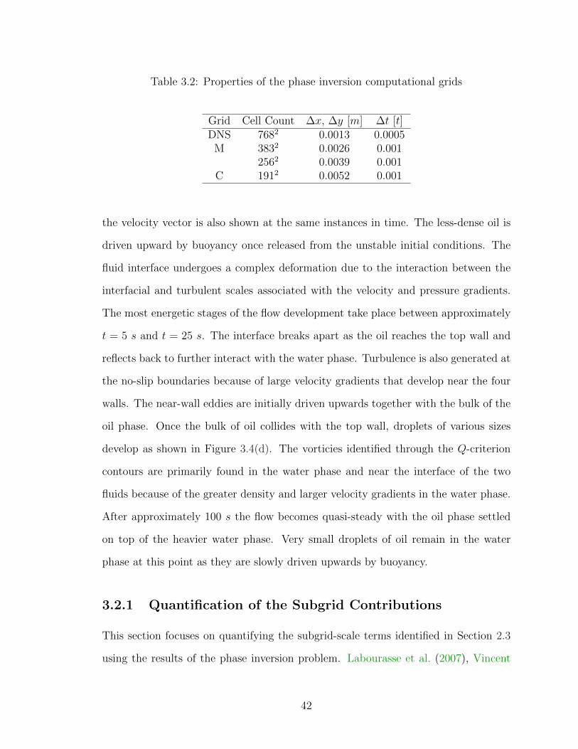
Table 3.2: Properties of the phase inversion computational grids
Grid Cell Count ∆x, ∆y [m] ∆t [t]DNS 7682 0.0013 0.0005
M 3832 0.0026 0.0012562 0.0039 0.001
C 1912 0.0052 0.001
the velocity vector is also shown at the same instances in time. The less-dense oil is
driven upward by buoyancy once released from the unstable initial conditions. The
fluid interface undergoes a complex deformation due to the interaction between the
interfacial and turbulent scales associated with the velocity and pressure gradients.
The most energetic stages of the flow development take place between approximately
t = 5 s and t = 25 s. The interface breaks apart as the oil reaches the top wall and
reflects back to further interact with the water phase. Turbulence is also generated at
the no-slip boundaries because of large velocity gradients that develop near the four
walls. The near-wall eddies are initially driven upwards together with the bulk of the
oil phase. Once the bulk of oil collides with the top wall, droplets of various sizes
develop as shown in Figure 3.4(d). The vorticies identified through the Q-criterion
contours are primarily found in the water phase and near the interface of the two
fluids because of the greater density and larger velocity gradients in the water phase.
After approximately 100 s the flow becomes quasi-steady with the oil phase settled
on top of the heavier water phase. Very small droplets of oil remain in the water
phase at this point as they are slowly driven upwards by buoyancy.
3.2.1 Quantification of the Subgrid Contributions
This section focuses on quantifying the subgrid-scale terms identified in Section 2.3
using the results of the phase inversion problem. Labourasse et al. (2007), Vincent
42
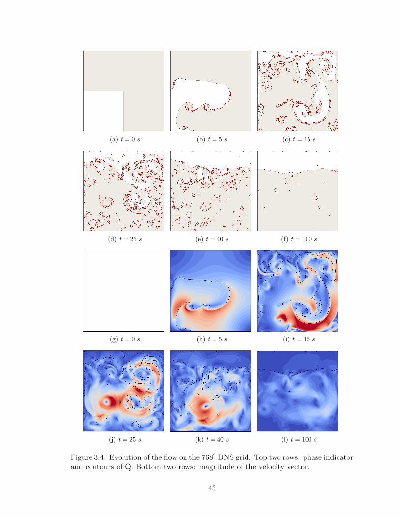
(a) t = 0 s (b) t = 5 s (c) t = 15 s
(d) t = 25 s (e) t = 40 s (f) t = 100 s
(g) t = 0 s (h) t = 5 s (i) t = 15 s
(j) t = 25 s (k) t = 40 s (l) t = 100 s
Figure 3.4: Evolution of the flow on the 7682 DNS grid. Top two rows: phase indicatorand contours of Q. Bottom two rows: magnitude of the velocity vector.
43
et al. (2008), and Larocque et al. (2010) have carried out a similar type of analysis of
this problem while employing different numerical simulation and SGS quantification
methods (see Section 2.3 for details).
Two sizes of the top-hat filter stencil are used: 3x3 (hereafter referred to as the
small filter, SF) and 5x5 (large filter, LF). By changing the size of the filter, each
subgrid term can be evaluated to determine its sensitivity to the change of the spa-
tial resolution of the computational grid used for large-eddy simulations. Increasing
of the filter-cutoff length-scale can be thought of as effectively using a coarser LES
grid in practice. The four subgrid-scale terms quantified include the traditional con-
vective term τC , diffusive term τD, acceleration term τA, and the interface term τI .
The contribution of each of the SGS terms to the discretized equations is examined
by quantifying the divergence of the convective term ∂τCij/∂xj, the diffusive term
∂τDij/∂xj, and the interface term ∂τI i/∂xi, as well as the time derivative of the
acceleration term ∂τAi/∂t. The surface tension SGS term is not considered in this
analysis because it has been shown by Larocque et al. (2010) to have a minor ef-
fect among the hierarchy of the other subgrid-scale terms. Additionally, Lakehal and
Liovic (2011) reports that for most types of breaking-wave flows, the SGS surface
tension contribution is several orders of magnitude smaller than the resolved compo-
nent due to the relatively negligible impact of the smallest scales on the total action
of the surface tension.
The time evolution of the four SGS terms obtained through the a priori procedure
is shown in Figure 3.5 for the first 40 seconds of the simulation time. During this
stage of the flow development, the largest dissipation rates and peak kinetic energy
occur. Additionally, the most complex flow features associated with the generation
of turbulence and the deformation of the interface also occur at this time.
At each sampled time, the maximum of each subgrid term contribution (∂τmax/∂xi
or ∂τmax/∂t) is computed and non-dimensionalized by the largest resolved term in the
44
appropriate governing equation. The y-component of the divergence of the resolved
convective acceleration ∂ρ uiuj/∂xj dominates the other resolved terms in magnitude
and hence the subgrid terms found in the momentum equation (∂τAi/∂t, ∂τCij/∂xj,
and ∂τDij/∂xj) are non-dimensionalized by ∂ρ u2uj/∂xj. Similarly, the resolved con-
vective term in the interface equation ∂u2α/∂x2 is used to non-dimensionalize the in-
terfacial subgrid term ∂τI i/∂xi. This form of normalization was adapted by Larocque
et al. (2010) and it was proven to give a valuable insight in the relative importance
of each subgrid-scale term.
The semi-log plots (Figure 3.5) illustrate several interesting trends. The vertical
component of the convective subgrid term is found to be the largest for the majority
of the simulation, reaching up to approximately 35% of the resolved component at
the most energetic stages of the flow. Its contribution is found to increase with the
application of the larger filter as also shown by Labourasse et al. (2007) and Larocque
et al. (2010). The two components of the diffusive SGS term behave similarly and
are found to be the second largest subgrid contributor to the momentum equation.
The contribution of the acceleration term is on the order of 10−4 of the maximum
resolved term, or over two orders of magnitude less than the convective and diffusive
terms. The importance of the interfacial term is found to increase when a larger filter
is used and its overall contribution to the maximum resolved term in the interface
equation is less than 3%.
In the first few seconds after the oil phase begins to rise due to buoyancy, the
diffusive SGS contribution increases relative to the other SGS terms. Because the
fluids are initially at rest in a highly-unstable condition, large velocity gradients form
immediately upon release and the difference between the subgrid velocity gradients
and the resolved gradients results in the diffusive SGS term’s relative magnitude. At
the same time, the subgrid interface term decreases in its contribution to the resolved
component until reaching its minimum value at t = 8 s. Before the bulk of the oil
45
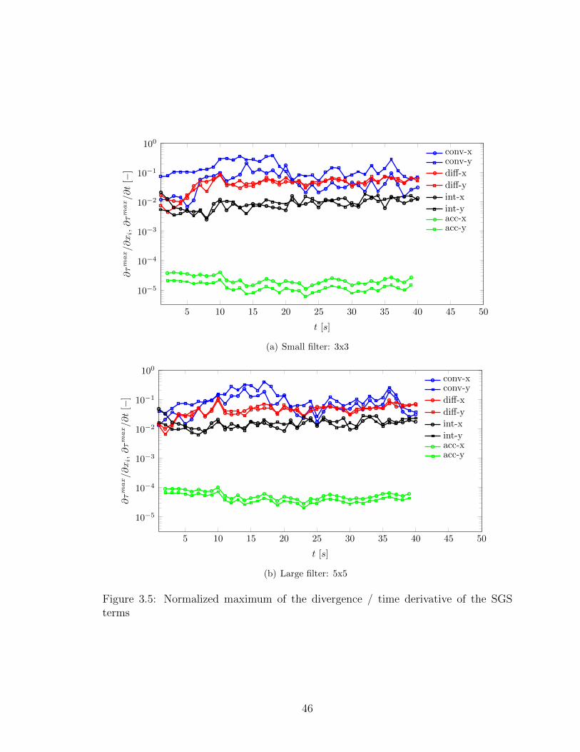
5 10 15 20 25 30 35 40 45 50
10−5
10−4
10−3
10−2
10−1
100
t [s]
∂τm
ax/∂xi,∂τm
ax/∂t
[−]
conv-xconv-y
diff-x
diff-yint-xint-yacc-xacc-y
(a) Small filter: 3x3
5 10 15 20 25 30 35 40 45 50
10−5
10−4
10−3
10−2
10−1
100
t [s]
∂τm
ax/∂xi,∂τm
ax/∂t
[−]
conv-xconv-y
diff-x
diff-yint-xint-yacc-xacc-y
(b) Large filter: 5x5
Figure 3.5: Normalized maximum of the divergence / time derivative of the SGSterms
46

reaches the top of the domain, the interface is well resolved and hence the subgrid
contribution is minimal. Once the oil impacts the top wall and small oil droplets form,
the subgrid interfacial term increases because a significant portion of the interfacial
structures are smaller than the filter cutoff. The acceleration term is affected by
the change of the filter size but its relative magnitude remains small throughout the
simulation, likely due to the very small size of the computational time-step used to
perform the direct numerical simulations.
In the next step of the analysis, contours of the magnitude of the four subgrid-
scale terms (|τC |, |τD|, |τA|, |τI |) are examined at three instances in time and as a
function of the filter size. It is important to understand the behavior of the subgird
terms and not just their relative size compared to the resolved terms of the governing
equations because it is the individual terms that are modeled in LES using the struc-
tural approach. The contours are presented in units of kg/m2s for τA, kg/ms2 for τC
and τD, and m/s for τI . The magnitude of a second-rank tensor is obtained using:
|A| =√AijAij (3.7)
where Aij is a generic symmetric tensor, and the magnitude of a vector is found using:
|B| =√BiBi (3.8)
where Bi represents a generic vector.
The diffusive stress contribution at t = 5 s is illustrated in Figure 3.6(a) using the
small filter stencil. The convective and acceleration subgrid terms are also included at
this time in Figure 3.6(b) and 3.6(c). The maximum diffusive subgrid stress is found in
a relatively small region of the oil phase near the left wall of the domain. At the latter
stages of the simulation, the subgrid diffusive term decreases in magnitude and its
contribution is mostly found near the oil-water interface as shown in Figures 3.6(d)
47
and 3.6(g). As expected, the overall subgrid contribution decreases with time as
the flow approaches a steady state. An increase of the filter stencil size results in the
diffusive SGS stress mostly retaining its relative magnitude as shown in Figure 3.5(b).
The contours of |τD| obtained using the 5x5 filter shown in Figures 3.7(d) and 3.7(g)
indicate that the diffusive SGS term becomes more active near the interface.
The convective subgrid term reaches its maximum contribution between 10 s <
t < 20 s once the bulk of the oil reaches the top of the domain. As the filter stencil is
increased, the convective SGS term increases and reaches up to 40% of the resolved
maximum. Figures 3.6(b), 3.6(e), and 3.6(h) show how the convective subgrid term
behaves at three instances in time. This term is found to be active in highly-vortical
regions and near the interface. In Figure 3.7(h), the contours of |τC | are relatively
small in magnitude but they populate the majority of the water phase where vorticies
and droplets of oil are present. A large portion of the turbulent structures is found
to be below the cutoff length of the large filter at this time.
The interface term is examined in Figure 3.8. As anticipated, this term is active
only in the diffuse-interface region where the value of the volume fraction α changes
between the oil and water phases. The application of the spatial filter in this region
results in an effective coarsening of the interface which in turn results in a loss of
interfacial detail. As the filter size is increased, the magnitude of the subgrid term
is found to increase rapidly. Figure 3.5 indicates that the ratio of ∂τI i/∂xi to its
resolved equivalent increases by approximately 50% when the large filter is used.
The interfacial subgrid term accounts for only approximately 1 to 3% of the resolved
term with the application of the large filter, but because its rate of change is higher
than of the other subgrid terms, the contribution of the interfacial term is likely to
be on the order of the convective SGS term on coarse LES grids. Additionally, the
fluid interface is governed by a separate equation from the Navier-Stokes equations,
allowing for a unique approach to the modeling of the subgrid interfacial term as part
48
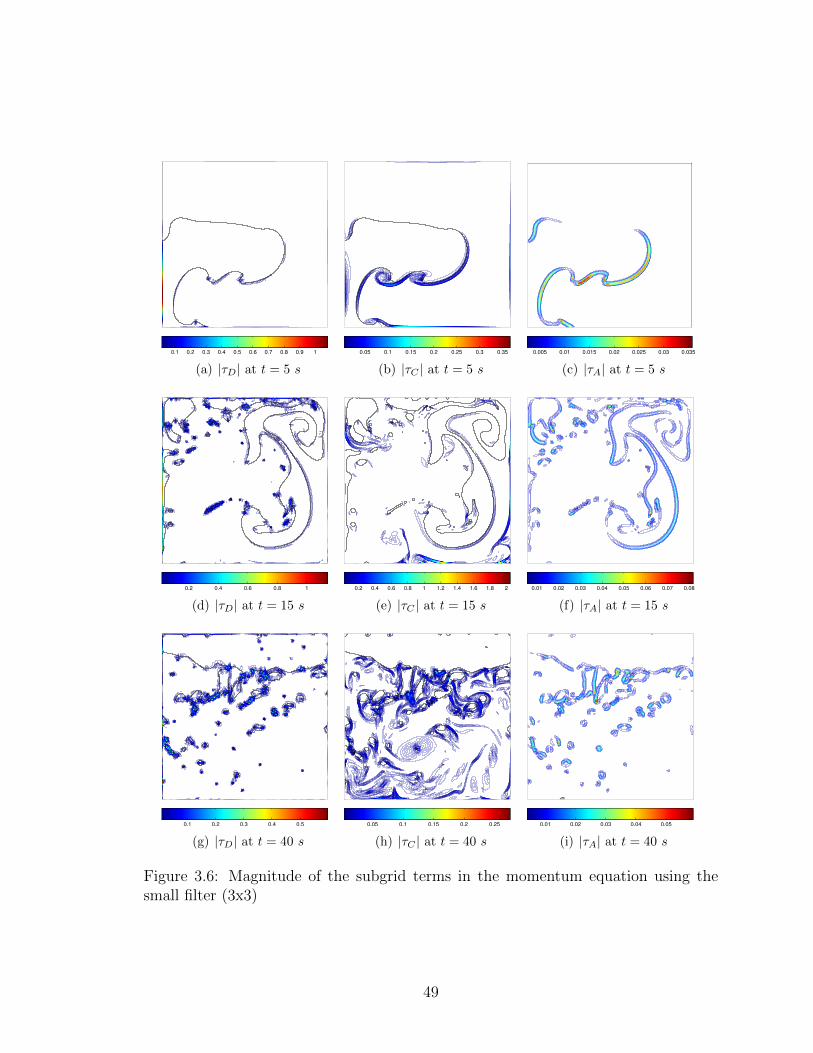
0.1 0.2 0.3 0.4 0.5 0.6 0.7 0.8 0.9 1
(a) |τD| at t = 5 s
0.05 0.1 0.15 0.2 0.25 0.3 0.35
(b) |τC | at t = 5 s
0.005 0.01 0.015 0.02 0.025 0.03 0.035
(c) |τA| at t = 5 s
0.2 0.4 0.6 0.8 1
(d) |τD| at t = 15 s
0.2 0.4 0.6 0.8 1 1.2 1.4 1.6 1.8 2
(e) |τC | at t = 15 s
0.01 0.02 0.03 0.04 0.05 0.06 0.07 0.08
(f) |τA| at t = 15 s
0.1 0.2 0.3 0.4 0.5
(g) |τD| at t = 40 s
0.05 0.1 0.15 0.2 0.25
(h) |τC | at t = 40 s
0.01 0.02 0.03 0.04 0.05
(i) |τA| at t = 40 s
Figure 3.6: Magnitude of the subgrid terms in the momentum equation using thesmall filter (3x3)
49
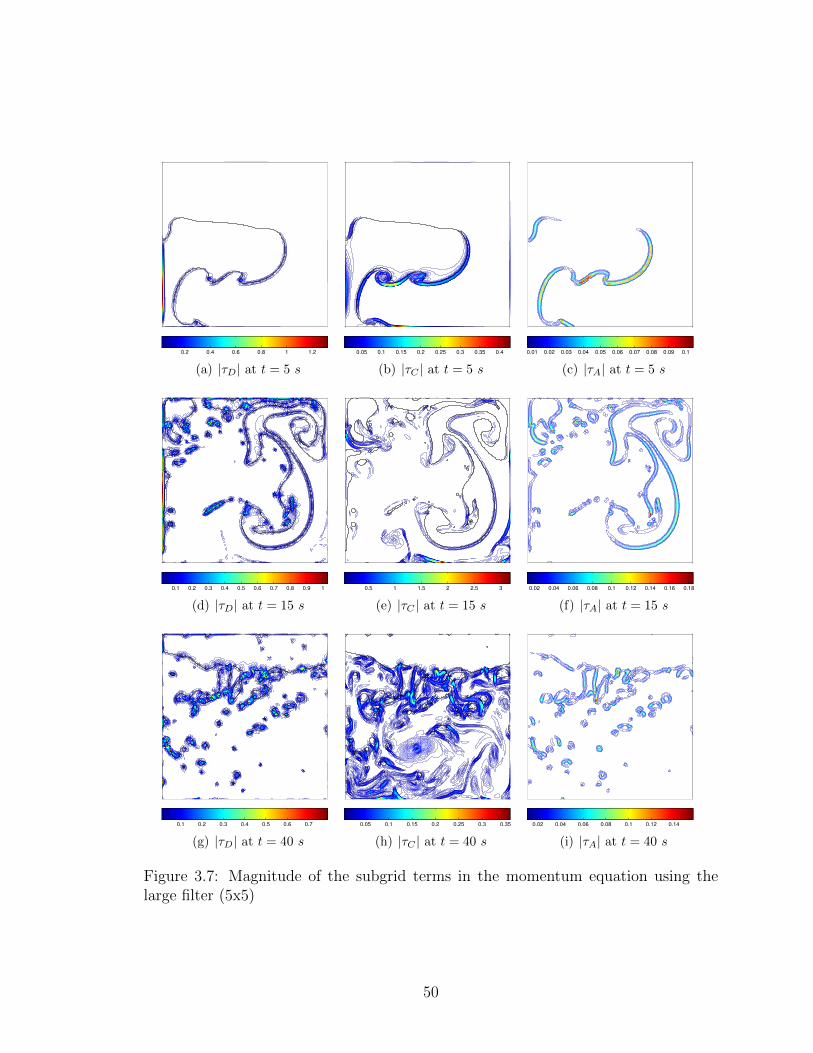
0.2 0.4 0.6 0.8 1 1.2
(a) |τD| at t = 5 s
0.05 0.1 0.15 0.2 0.25 0.3 0.35 0.4
(b) |τC | at t = 5 s
0.01 0.02 0.03 0.04 0.05 0.06 0.07 0.08 0.09 0.1
(c) |τA| at t = 5 s
0.1 0.2 0.3 0.4 0.5 0.6 0.7 0.8 0.9 1
(d) |τD| at t = 15 s
0.5 1 1.5 2 2.5 3
(e) |τC | at t = 15 s
0.02 0.04 0.06 0.08 0.1 0.12 0.14 0.16 0.18
(f) |τA| at t = 15 s
0.1 0.2 0.3 0.4 0.5 0.6 0.7
(g) |τD| at t = 40 s
0.05 0.1 0.15 0.2 0.25 0.3 0.35
(h) |τC | at t = 40 s
0.02 0.04 0.06 0.08 0.1 0.12 0.14
(i) |τA| at t = 40 s
Figure 3.7: Magnitude of the subgrid terms in the momentum equation using thelarge filter (5x5)
50
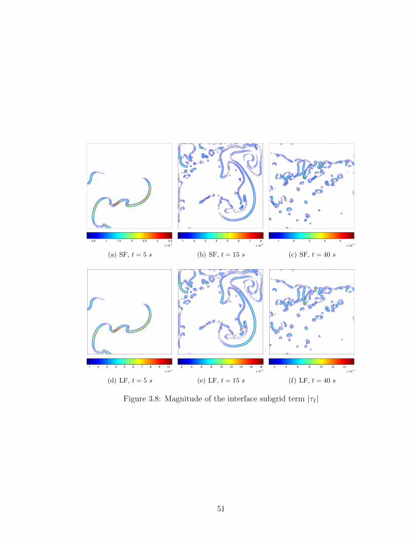
0.5 1 1.5 2 2.5 3 3.5
x 10−4
(a) SF, t = 5 s
1 2 3 4 5 6 7 8
x 10−4
(b) SF, t = 15 s
1 2 3 4 5
x 10−4
(c) SF, t = 40 s
1 2 3 4 5 6 7 8 9 10
x 10−4
(d) LF, t = 5 s
2 4 6 8 10 12 14 16 18
x 10−4
(e) LF, t = 15 s
2 4 6 8 10 12 14
x 10−4
(f) LF, t = 40 s
Figure 3.8: Magnitude of the interface subgrid term |τI |
51
of the interface equation.
3.2.2 Modeling of the Subgrid-Scale Terms
In this section, the subgrid-scale terms are modeled using the filtered DNS data of the
phase-inversion problem. The filtered data available on the LES grid level is used to
compute the contribution of the tested LES models, as described in Chapter 2. The
a priori testing of the SGS models allows for an insight into the model’s ability to
replicate the interaction of the resolved and subgrid scales. The traditional convective
SGS stress tensor τC is modeled using the dynamic Smagorinsky, the scale-similarity,
and the stress-similarity models. The original scale-similarity model of Bardina et al.
(1980) is compared to its generalized version or the stress-similarity model introduced
by Liu et al. (1994). The two similarity-based models and the dynamic eddy-viscosity
model are also used as a proxy to evaluate the potential benefit of the mixed SGS
modeling that combines an eddy-viscosity contribution with a similarity-type contri-
bution. The stress-similarity concept is extended to the modeling of the diffusive, the
acceleration, and the interfacial subgrid-scale terms.
The performance of each model is evaluated based on the correlation coefficients
between the real subgrid stresses and the modeled stresses. This approach is based
on the work of Liu et al. (1994) that involved the study of turbulence in a round
jet, as well as the work of Chesnel et al. (2011a) which focused on spray-atomization
problems. The magnitude of each subgrid term (see Equations 3.7 and 3.8) is used
for the correlation coefficient calculation to simplify the analysis. The correlation
coefficient r for two variables a and b is found using:
r =〈ab〉 − 〈a〉〈b〉√
(〈a2〉 − 〈a〉2) (〈b2〉 − 〈b〉2)(3.9)
where 〈〉 is the mean. The coefficient can vary between -1 indicating negative corre-
52
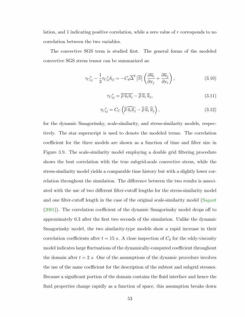
lation, and 1 indicating positive correlation, while a zero value of r corresponds to no
correlation between the two variables.
The convective SGS term is studied first. The general forms of the modeled
convective SGS stress tensor can be summarized as:
τC∗ij −
1
3τC∗iiδij = −Cd∆
2 ∣∣S∣∣ (∂ui∂xj
+∂uj∂xi
), (3.10)
τC∗ij = ρ uiuj − ρ ui uj, (3.11)
τC∗ij = CC
(ρ uiuj − ρ ui uj
), (3.12)
for the dynamic Smagorinsky, scale-similarity, and stress-similarity models, respec-
tively. The star superscript is used to denote the modeled terms. The correlation
coefficient for the three models are shown as a function of time and filter size in
Figure 3.9. The scale-similarity model employing a double grid filtering procedure
shows the best correlation with the true subgrid-scale convective stress, while the
stress-similarity model yields a comparable time history but with a slightly lower cor-
relation throughout the simulation. The difference between the two results is associ-
ated with the use of two different filter-cutoff lengths for the stress-similarity model
and one filter-cutoff length in the case of the original scale-similarity model (Sagaut
(2001)). The correlation coefficient of the dynamic Smagorinsky model drops off to
approximately 0.3 after the first two seconds of the simulation. Unlike the dynamic
Smagorinsky model, the two similarity-type models show a rapid increase in their
correlation coefficients after t = 15 s. A close inspection of Cd for the eddy-viscosity
model indicates large fluctuations of the dynamically-computed coefficient throughout
the domain after t = 2 s. One of the assumptions of the dynamic procedure involves
the use of the same coefficient for the description of the subtest and subgrid stresses.
Because a significant portion of the domain contains the fluid interface and hence the
fluid properties change rapidly as a function of space, this assumption breaks down
53
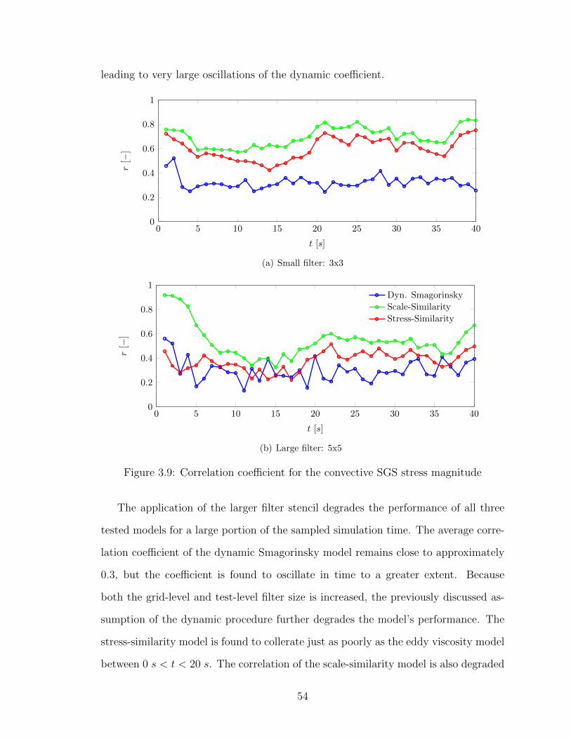
leading to very large oscillations of the dynamic coefficient.
0 5 10 15 20 25 30 35 400
0.2
0.4
0.6
0.8
1
t [s]
r[−
]
(a) Small filter: 3x3
0 5 10 15 20 25 30 35 400
0.2
0.4
0.6
0.8
1
t [s]
r[−
]
Dyn. Smagorinsky
Scale-Similarity
Stress-Similarity
(b) Large filter: 5x5
Figure 3.9: Correlation coefficient for the convective SGS stress magnitude
The application of the larger filter stencil degrades the performance of all three
tested models for a large portion of the sampled simulation time. The average corre-
lation coefficient of the dynamic Smagorinsky model remains close to approximately
0.3, but the coefficient is found to oscillate in time to a greater extent. Because
both the grid-level and test-level filter size is increased, the previously discussed as-
sumption of the dynamic procedure further degrades the model’s performance. The
stress-similarity model is found to collerate just as poorly as the eddy viscosity model
between 0 s < t < 20 s. The correlation of the scale-similarity model is also degraded
54

during this time, reaching a low of approximately 0.35 at t = 15 s. The use of the
large filter stencil effectively corresponds to an LES grid with 1282 cells. The rela-
tively coarse grid is then test filtered using a stencil size based on ∆ = 2∆, resulting
in a poor estimation for the test-level stress from the grid-filtered information. This
behavior will be examined further as part of the following analysis.
The stress-similarity model with constant coefficients is now used to compute the
modeled subgrid contribution of the acceleration, the interfacial, and the diffusive
terms. The terms are modeled using:
τA∗i = CA
(ρ ui − ρ ui
), (3.13)
τI∗i = CI
(ui α− ui α
), (3.14)
τD∗ij = CD
(M −N
), (3.15)
where
M = µ
(∂ui∂xj
+∂uj∂xi
)(3.16)
N = µ
(∂ui∂xj
+∂uj∂xi
)(3.17)
and CA, CI , CD are the stress-similarity coefficients set equal to one based on the
arguments presented in Section 2.2.2. The convective term modeled using stress-
similarity (Equation 3.12) is also included as a reference. The correlation coefficients
for the four subgrid stresses are included in Figure 3.10(a) for the small filter and
in Figure 3.10(b) for the large filter. It is worthwhile to point out that the interface
and the acceleration terms have the same correlation coefficient and hence the two
lines overlap in the plots. This result is due to the definitions of the two terms and
of the correlation coefficient. The acceleration term involves products of the filtered
velocity field and the filtered density while the interface term contains products of the
55
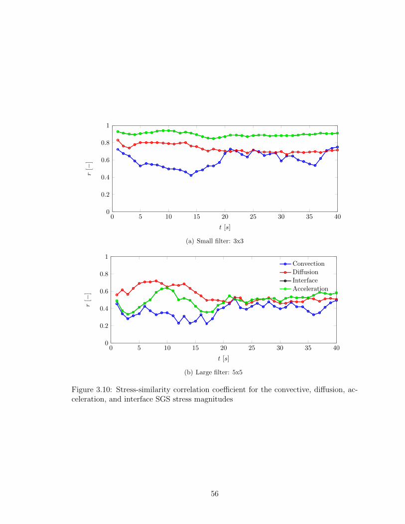
0 5 10 15 20 25 30 35 400
0.2
0.4
0.6
0.8
1
t [s]
r[−
]
(a) Small filter: 3x3
0 5 10 15 20 25 30 35 400
0.2
0.4
0.6
0.8
1
t [s]
r[−
]
Convection
Diffusion
Interface
Acceleration
(b) Large filter: 5x5
Figure 3.10: Stress-similarity correlation coefficient for the convective, diffusion, ac-celeration, and interface SGS stress magnitudes
56

filtered velocity field and the filtered volume fraction. The density and the volume
fraction fields are only different in magnitude and units because the density field is
a function of the volume fraction (see Equation 2.36). The correlation coefficients of
the interface and acceleration terms stay between 0.8 and 1.0 for the entire sampled
simulation time when the small filter stencil is applied, indicating that the test-level
information adequately models the subgrid stresses. The correlation of the two terms
is significantly reduced to an average value of approximately 0.5 by filtering the DNS
data with a greater filter-cutoff length. A similar trend of the correlation coefficient
degradation is found for the diffusive and convective terms modeled with the stress-
similarity approach.
The effects of the filter size on the robustness of the stress-similarity model can
be studied further by examining the modeled contribution directly and comparing it
to the true subgrid term obtained from the DNS data. The analysis is carried out
for the interface SGS term only at three instances in time (t = 5, 15, 40 s), but
the findings are directly relevant to the other SGS stresses modeled with the stress-
similarity technique. Contours of |τI | are compared to the contours of the modeled
term |τI∗| in Figure 3.11. The small grid filter is used and the stress-similarity model
utilizes a secondary test-level filter that is twice the size of the grid filter (∆ = 2∆).
A close inspection of the results shows that the model is active in the appropriate
regions of the domain where the true SGS term is present. At t = 5 s and t = 15 s, the
maximum of the modeled contribution is between two to three times greater than the
maximum of the true subgrid term, but the locations of the peak subgrid contribution
are reproduced well by the model. Based on these findings, a dynamic determination
of the stress-similarity coefficient or an adjustment to the ratio between the test and
grid filter cutoff could be beneficial to the prediction of the correct magnitude of the
modeled contribution.
Figure 3.12 illustrates the limitation of the test-filtering procedure that is at the
57
0.5 1 1.5 2 2.5 3 3.5
x 10−4
(a) |τI | at t = 5 s
1 2 3 4 5 6 7 8
x 10−4
(b) |τI | at t = 15 s
1 2 3 4 5
x 10−4
(c) |τI | at t = 40 s
2 4 6 8 10 12 14
x 10−4
(d) |τI∗| at t = 5 s
0.5 1 1.5 2 2.5
x 10−3
(e) |τI∗| at t = 15 s
0.5 1 1.5 2
x 10−3
(f) |τI∗| at t = 40 s
Figure 3.11: Magnitude of the true interface subgrid term |τI | and the modeled con-tribution |τI∗| using the stress-similarity approach. Small filter (3x3) and CI = 1.
58
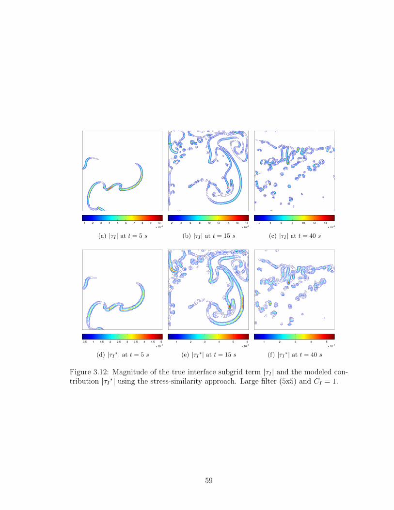
1 2 3 4 5 6 7 8 9 10
x 10−4
(a) |τI | at t = 5 s
2 4 6 8 10 12 14 16 18
x 10−4
(b) |τI | at t = 15 s
2 4 6 8 10 12 14
x 10−4
(c) |τI | at t = 40 s
0.5 1 1.5 2 2.5 3 3.5 4 4.5 5
x 10−3
(d) |τI∗| at t = 5 s
1 2 3 4 5 6
x 10−3
(e) |τI∗| at t = 15 s
1 2 3 4 5
x 10−3
(f) |τI∗| at t = 40 s
Figure 3.12: Magnitude of the true interface subgrid term |τI | and the modeled con-tribution |τI∗| using the stress-similarity approach. Large filter (5x5) and CI = 1.
59
core of the stress-similarity model. The grid filter is now increased to the 5x5 stencil
and the test-level filter is increased accordingly. The magnitude of the true subgrid
stress is found to increase as previously shown, but the contribution of the model
is poorly correlated with the true SGS stress in terms of magnitude and location
in the domain. The peak contribution is more than an order of magnitude smaller
at all three instances in time and the flow information available on the test-filter
level is not sufficiently resolved to model the subgrid term. The locations of the
peak model contribution at the fluid interface no longer match the locations of the
peak magnitude of |τI | and the modeled subgrid stress appears heavily smeared and
contaminated with spurious information.
Highly-resolved simulations of the phase-inversion problem are used to determine
the hierarchy of the subgrid-scale terms present in the governing equations. The
convective term is found to be the largest subgrid contributor relative to the resolved
quantities, but the diffusive and the interfacial subgrid terms can also be significant.
The acceleration term is the smallest subgrid contributor regardless of the filter size
used. The interfacial term rapidly increases in magnitude with the increase of the
filter stencil. The stress-similarity-based modeling of the subgrid terms is found to
correlate well with the true subgrid behavior, but the correlation degrades as the filter
size is increased.
3.3 Plunging-Breaking Wave
In this section, a plunging-breaking water wave is examined using high-resolution nu-
merical simulations. The plunging-breaking wave flow shares some important charac-
teristics with the phase-inversion problem, but the greater fluid density and viscosity
ratios used in the wave-breaking problem introduce new unknowns and challenges
in the understanding of the interface-turbulence interaction. The results presented
60

here are based on the work of Iafrati (2009, 2011) and Iafrati et al. (2012) where
two-dimensional simulations are used to study the early stages of wave breaking. In
those works, several modes of breaking are investigated ranging from a weak-spilling
type to a strong-plunging type depending on the initial conditions used.
A similar simulation technique is used here to extend on the previously-published
two-dimensional results. An artificially-steep wave is initialized in a domain with pe-
riodic boundaries in the streamwise direction and no-slip top and bottom boundaries.
The periodic boundaries and the wave initialization at t = 0 s allow for a significant
savings in terms of computational expense because the dispersive focusing of a set of
waves does not need to be simulated to obtain the initial conditions of interest. This
approach for simulating water waves has also been adapoted in Song and Sirviente
(2004) and Lubin (2004) among others. Three-dimensional simulations are conducted
using a computational domain shown in Figure 3.13 with dimensions of λ× λ× λ/2
(in the x, y, and z directions, respectively) and where the lateral boundaries are
also periodic. Stokes’s third-order wave theory is used to initialize the free-surface
elevation η and the streamwise and vertical water-particle velocities u, v using:
η(x, 0) =A
λ
(cos(kx) +
1
2σ cos(2kx) +
3
8σ2 cos(3kx)
), (3.18)
u(x, y, 0) = ΩAeky cos(kx), (3.19)
v(x, y, 0) = ΩAeky sin(kx), (3.20)
where σ = Ak is the wave steepness and Ω =√gk (1 + σ2) is the wave frequency cor-
rected for nonlinear effects as shown in Whitham (1974). The wave train is simulated
in deep water with h/λ = 0.5 resulting in negligible effects of the no-slip bottom on
the evolution of the wave-breaking process.
Parameters of air and water are included in Table 3.3 and both phases are assumed
61
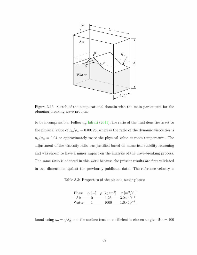
Figure 3.13: Sketch of the computational domain with the main parameters for theplunging-breaking wave problem
to be incompressible. Following Iafrati (2011), the ratio of the fluid densities is set to
the physical value of ρa/ρw = 0.00125, whereas the ratio of the dynamic viscosities is
µa/µw = 0.04 or approximately twice the physical value at room temperature. The
adjustment of the viscosity ratio was justified based on numerical stability reasoning
and was shown to have a minor impact on the analysis of the wave-breaking process.
The same ratio is adapted in this work because the present results are first validated
in two dimensions against the previously-published data. The reference velocity is
Table 3.3: Properties of the air and water phases
Phase α [−] ρ [kg/m3] ν [m2/s]Air 0 1.25 3.2×10⁻³
Water 1 1000 1.0×10⁻⁴
found using u0 =√λg and the surface tension coefficient is chosen to give We = 100
62
using:
We = g1/2λ
√ρwγ. (3.21)
Selecting this Weber number corresponds to simulating a wave with λ = 0.27 m,
the Reynolds number in water is set to Rew = 10, 000, and the Froude number is
Fr = 1.0.
3.3.1 Validation Study
The resolution of the smallest scales of turbulence necessary to conduct direct nu-
merical simulations is first verified using two-dimensional simulations. Two types of
breaking are studied: a spilling-breaking wave with an initial steepness of σ = 0.35
as well as a plunging-breaking wave with a steepness of σ = 0.60. The reference grid
is selected to have 512 uniformly-spaced cells in the streamwise and vertical direc-
tions based on the previously-published results. One coarser grid with 2562 cells and
two finer grids with 10242 and 20482 uniformly-spaced cells are also constructed. All
simulations span six wave periods defined as T =√gk.
The simulations are carried out using second-order numerical schemes and the
interface capturing method described in Section 3.1. The interface is spread across
approximately 1% of the wave length. The influence of the interface thickness was
examined by comparing the global flow quantities with the thickness varying between
0.2% and 3% of wave length on the finest grid. Negligible differences of the global
quantities such as the total energy in the domain and each phase were found across
all tested interface thicknesses. Further analysis of the impact of the diffuse-interface
technique can be found in Iafrati (2009).
The mechanical energy is each phase is found by summing the kinetic and potential
63
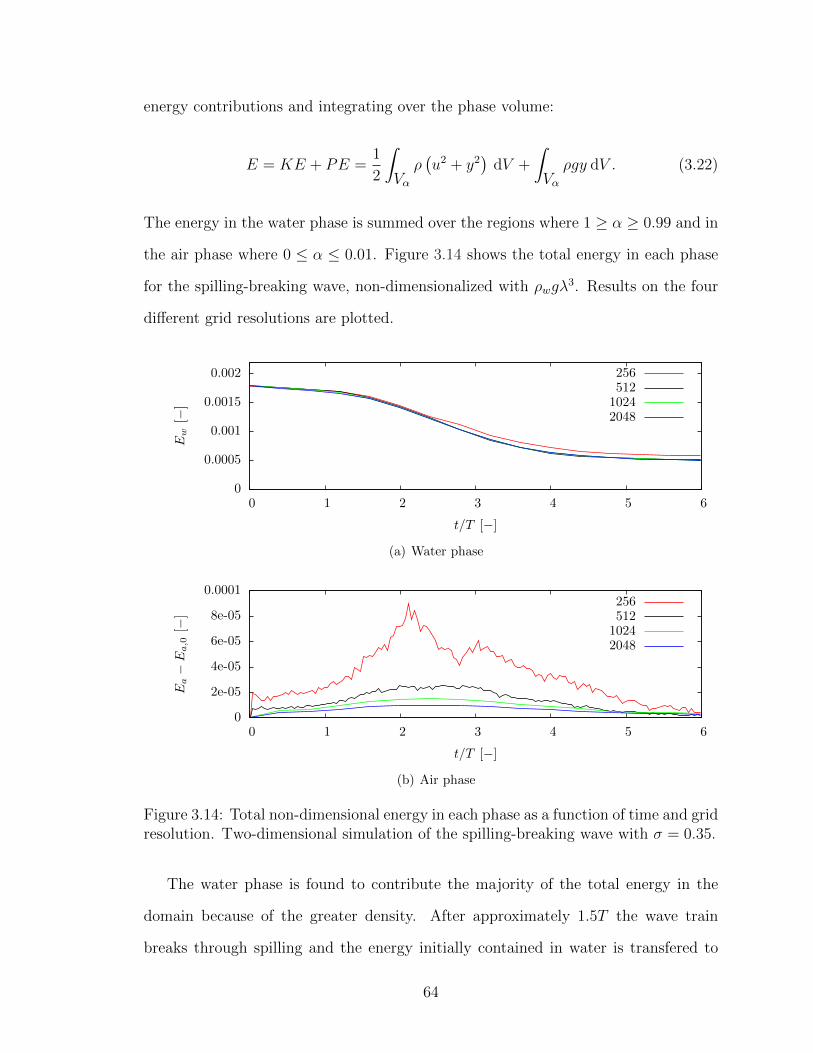
energy contributions and integrating over the phase volume:
E = KE + PE =1
2
∫Vα
ρ(u2 + y2
)dV +
∫Vα
ρgy dV . (3.22)
The energy in the water phase is summed over the regions where 1 ≥ α ≥ 0.99 and in
the air phase where 0 ≤ α ≤ 0.01. Figure 3.14 shows the total energy in each phase
for the spilling-breaking wave, non-dimensionalized with ρwgλ3. Results on the four
different grid resolutions are plotted.
0
0.0005
0.001
0.0015
0.002
0 1 2 3 4 5 6
Ew
[−]
t/T [−]
256512
10242048
(a) Water phase
0
2e-05
4e-05
6e-05
8e-05
0.0001
0 1 2 3 4 5 6
Ea−E
a,0
[−]
t/T [−]
256512
10242048
(b) Air phase
Figure 3.14: Total non-dimensional energy in each phase as a function of time and gridresolution. Two-dimensional simulation of the spilling-breaking wave with σ = 0.35.
The water phase is found to contribute the majority of the total energy in the
domain because of the greater density. After approximately 1.5T the wave train
breaks through spilling and the energy initially contained in water is transfered to
64
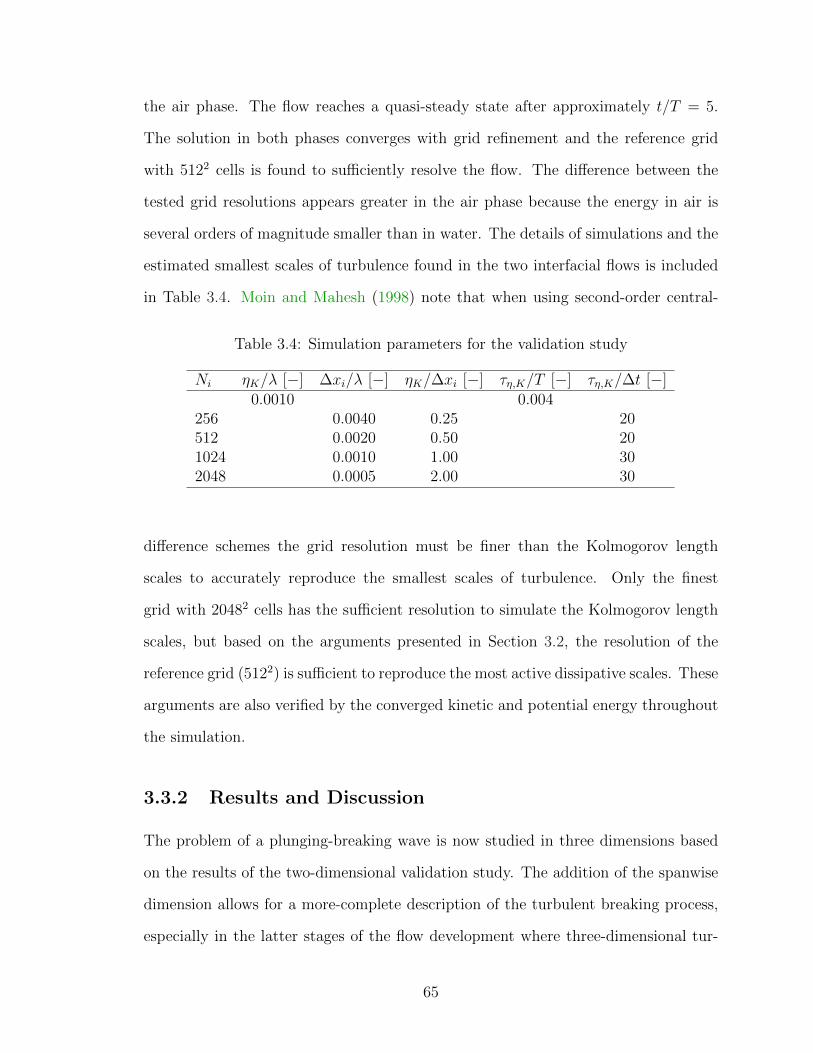
the air phase. The flow reaches a quasi-steady state after approximately t/T = 5.
The solution in both phases converges with grid refinement and the reference grid
with 5122 cells is found to sufficiently resolve the flow. The difference between the
tested grid resolutions appears greater in the air phase because the energy in air is
several orders of magnitude smaller than in water. The details of simulations and the
estimated smallest scales of turbulence found in the two interfacial flows is included
in Table 3.4. Moin and Mahesh (1998) note that when using second-order central-
Table 3.4: Simulation parameters for the validation study
Ni ηK/λ [−] ∆xi/λ [−] ηK/∆xi [−] τη,K/T [−] τη,K/∆t [−]0.0010 0.004
256 0.0040 0.25 20512 0.0020 0.50 201024 0.0010 1.00 302048 0.0005 2.00 30
difference schemes the grid resolution must be finer than the Kolmogorov length
scales to accurately reproduce the smallest scales of turbulence. Only the finest
grid with 20482 cells has the sufficient resolution to simulate the Kolmogorov length
scales, but based on the arguments presented in Section 3.2, the resolution of the
reference grid (5122) is sufficient to reproduce the most active dissipative scales. These
arguments are also verified by the converged kinetic and potential energy throughout
the simulation.
3.3.2 Results and Discussion
The problem of a plunging-breaking wave is now studied in three dimensions based
on the results of the two-dimensional validation study. The addition of the spanwise
dimension allows for a more-complete description of the turbulent breaking process,
especially in the latter stages of the flow development where three-dimensional tur-
65
bulent and interfacial structures are important (Iafrati (2011); Lubin et al. (2006)).
The domain spans over 0.5λ in the z-direction and is discretized with 512 cells in
the streamwise and vertical directions, and 256 cells in the spanwise direction. The
cells are uniformly spaced in all directions. The selected discretization of the domain
is based on the two-dimensional validation study where the results obtained on the
reference grid with 5122 cells were shown to be converged. Lubin et al. (2006) reports
a slight increase in the dissipation rate of a three-dimensional plunging breaker com-
pared to a two-dimensional simulation but the grid resolution used here is sufficient
to resolve at least the early stages of the breaking process because the increase in the
dissipation rate was found in the post-breaking stages of the flow development. The
three-dimensional simulations are conducted on a grid with over 67 million cells and
approximately 1,100 computational cores were used to execute the simulations over
144 hours on the Lonestar High Performance Computing (HPC) cluster. The Lon-
estar HPC is part of the Extreme Science and Engineering Discovery Environment
(XSEDE) and the cluster consist of over 22,000 modern computational cores with 44
terabytes of total memory and a peak performance of 302 teraflops.
The initial free-surface profile and the early stages of the breaking process are
shown on a centerline plane in Figure 3.15. Several contours of the second invariant
of the velocity gradient tensor Q and the magnitude of the velocity vector are also
included. The identified turbulent structures are found to remain in close proximity to
the fluid interface and to the entrained air cavities. The peak velocities are located in
the region of the jet splash-up and where the overturning jet collapses. The magnitude
of the velocity decreases rapidly away from the interface, resulting in large gradients
of velocity in both phases.
The evolution of the potential and the kinetic energy in the water phase is shown
in Figure 3.16. The total kinetic energy in the domain including the air phase is
also shown. The bulk of the kinetic energy is contained within the water phase. The
66

(a) t/T = 0.0 (b) t/T = 0.6 (c) t/T = 1.2
(d) t/T = 0.0 (e) t/T = 0.6 (f) t/T = 1.2
Figure 3.15: Evolution of the plunging-breaker flow on the DNS grid. Top row: darkgray regions represent the water phase and the contours of the second invariant ofthe velocity gradient tensor Q are shown in red. Bottom row: magnitude of velocityvector.
0
0.002
0.004
0.006
0.008
0.01
0.012
0 1 2 3 4 5 6
E/(ρwu02V/2)
[−]
t/T [−]
KE domainKE waterPE water
Figure 3.16: Time evolution of the potential and kinetic energy of the three-dimensional plunging-breaking wave
67
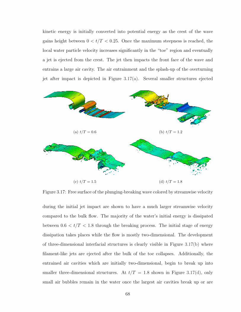
kinetic energy is initially converted into potential energy as the crest of the wave
gains height between 0 < t/T < 0.25. Once the maximum steepness is reached, the
local water particle velocity increases significantly in the “toe” region and eventually
a jet is ejected from the crest. The jet then impacts the front face of the wave and
entrains a large air cavity. The air entrainment and the splash-up of the overturning
jet after impact is depicted in Figure 3.17(a). Several smaller structures ejected
(a) t/T = 0.6 (b) t/T = 1.2
(c) t/T = 1.5 (d) t/T = 1.8
Figure 3.17: Free surface of the plunging-breaking wave colored by streamwise velocity
during the initial jet impact are shown to have a much larger streamwise velocity
compared to the bulk flow. The majority of the water’s initial energy is dissipated
between 0.6 < t/T < 1.8 through the breaking process. The initial stage of energy
dissipation takes places while the flow is mostly two-dimensional. The development
of three-dimensional interfacial structures is clearly visible in Figure 3.17(b) where
filament-like jets are ejected after the bulk of the toe collapses. Additionally, the
entrained air cavities which are initially two-dimensional, begin to break up into
smaller three-dimensional structures. At t/T = 1.8 shown in Figure 3.17(d), only
small air bubbles remain in the water once the largest air cavities break up or are
68

driven towards to the free surface by buoyancy. The major features of the breaking
process including the toe formation, jet ejection and splash-up, and the exponential
decay of the wave’s energy is found to be reproduced well in the present simulation
compared to the documented studies of plunging-breaking waves.
3.3.3 Quantification of the Subgrid Contributions
The subgrid contribution is now quantified for the plunging-breaking wave flow through
the a priori approach. The a priori analysis of the direct numerical simulation data is
conducted in the same consistent manner as previously shown for the phase-inversion
problem. To the author’s knowledge, this type of analysis of a plunging-breaking
water wave has not been previously published.
The top-hat filter stencils are now three dimensional to account for the spanwise
extent of the computational domain. The small filter uses a 3x3x3 stencil and the
large filter uses a 5x5x5 stencil. The same four subgrid-scale terms are studied as
in the phase-inversion problem of Section 3.2: τC , τD, τA, and τI . The contribution
of each of the subgrid terms to the corresponding discretized governing equations is
studied by quantifying the divergence of the spatial terms and the time derivative of
the acceleration term (∂τCij/∂xj, ∂τDij/∂xj, ∂τAi/∂t, and ∂τI i/∂xi). The maximum
of each subgrid contribution (∂τijmax/∂xi or ∂τij
max/∂t) is computed at each sampled
time for the duration of the simulation. The maxima are then non-dimensionalized
by the largest resolved term in the corresponding governing equation. In the case of
the momentum equation, the vertical component of the resolved convective acceler-
ation ∂ρ u2uj/∂xj is used, whereas in the interface equation, ∂u2α/∂x2 is used for
normalization of the subgrid contributions. The non-dimensionalize process follows
the work of Larocque et al. (2010) and is consistent with the approach used for the
phase-inversion a priori study.
The three normalized components of each studied subgrid term are plotted in
69
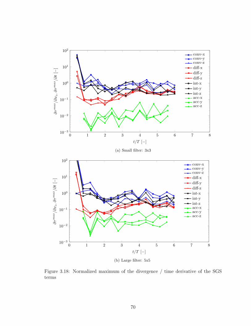
0 1 2 3 4 5 6 7 810−3
10−2
10−1
100
101
102
t/T [−]
∂τm
ax/∂xi,∂τm
ax/∂t
[−]
conv-xconv-yconv-z
diff-x
diff-y
diff-zint-xint-yint-zacc-xacc-yacc-z
(a) Small filter: 3x3
0 1 2 3 4 5 6 7 810−3
10−2
10−1
100
101
102
t/T [−]
∂τm
ax/∂xi,∂τm
ax/∂t
[−]
conv-xconv-yconv-z
diff-x
diff-y
diff-zint-xint-yint-zacc-xacc-yacc-z
(b) Large filter: 5x5
Figure 3.18: Normalized maximum of the divergence / time derivative of the SGSterms
70

Figure 3.18 for both filter sizes. The most energetic stage of the wave-breaking process
takes place between 0.4 < t/T < 2.4. The most significant changes of the subgrid
term contributions also occur during this time. The maximum of the convective
and the interfacial SGS terms are found to be on the order of magnitude of the
resolved contributions for the majority of the simulation, and to be the largest subgrid
contributors at the time of breaking. The diffusive SGS term is much less active during
the breaking process and it remains smaller than the convective SGS contribution at
most instances in time. The acceleration subgrid term is once again found to have
the smallest contribution to the momentum equation. It is worthwhile pointing out
that Chesnel et al. (2011a) investigated this term’s relative contribution for the spray-
atomization problem and as a function of the order of the time-integration scheme
used. The authors found that the relative contribution of the acceleration term was
not affected by the order of the numerical scheme, and hence the order of the temporal
scheme used in this work is unlikely to affect the term’s magnitude.
At the first sampled time of t/T = 0.4, the streamwise and the vertical components
of the convective, diffusive, and interfacial SGS terms dominate the corresponding
resolved terms. The same trend is found when the larger grid filter is used as shown
in Figure 3.18(b). The relatively small magnitude of the resolved convective terms
in the momentum and interface equations at this point in the flow’s development is
responsible for the relative subgrid contributions. The normalized subgrid terms are
drastically reduced at the next sampled time (t/T = 0.8) once the magnitude of the
resolved terms increases with the evolution of the wave-breaking process. At the time
of the jet splash-up and the formation of three-dimensional interfacial structures,
the z-component of the interfacial SGS term becomes more important relative to
the resolved interfacial component. Once the flow begins to settle and approaches a
steady state after approximately t/T = 4, the magnitude of the spanwise components
of the subgrid terms decreases.
71

0.5 1 1.5 2
(a) |τD| at t/T = 0.4
5 10 15 20 25
(b) |τC | at t/T = 0.4
2 4 6 8 10 12 14 16
(c) |τA| at t/T = 0.4
0.5 1 1.5 2 2.5 3 3.5 4 4.5 5
(d) |τD| at t/T = 1.2
10 20 30 40 50 60 70 80 90
(e) |τC | at t/T = 1.2
10 20 30 40 50 60 70 80
(f) |τA| at t/T = 1.2
0.05 0.1 0.15 0.2 0.25 0.3 0.35 0.4 0.45 0.5
(g) |τD| at t/T = 4.8
0.2 0.4 0.6 0.8 1 1.2 1.4 1.6
(h) |τC | at t/T = 4.8
0.5 1 1.5 2 2.5 3
(i) |τA| at t/T = 4.8
Figure 3.19: Magnitude of the subgrid terms in the momentum equation using thesmall filter (3x3x3). Center-plane at z = 0.5W .
72

0.5 1 1.5 2 2.5 3
(a) |τD| at t/T = 0.4
10 20 30 40 50 60
(b) |τC | at t/T = 0.4
5 10 15 20 25 30 35 40 45
(c) |τA| at t/T = 0.4
1 2 3 4 5 6
(d) |τD| at t/T = 1.2
20 40 60 80 100 120 140
(e) |τC | at t/T = 1.2
10 20 30 40 50 60 70 80
(f) |τA| at t/T = 1.2
0.05 0.1 0.15 0.2 0.25
(g) |τD| at t/T = 4.8
0.2 0.4 0.6 0.8 1 1.2 1.4 1.6 1.8 2
(h) |τC | at t/T = 4.8
0.5 1 1.5 2 2.5 3 3.5 4 4.5
(i) |τA| at t/T = 4.8
Figure 3.20: Magnitude of the subgrid terms in the momentum equation using thelarge filter (5x5x5). Center-plane at z = 0.5W .
73
The overall subgrid contribution from the four terms tends to increase with the
increase of the filter-cutoff length. The SGS terms tend to be highly localized near the
interface, especially before the impact of the overturning jet. Large particle velocities
in the toe region result in the subgrid terms becoming highly active in the early
stages of the breaking process. The subgrid terms from the momentum equation
(τC , τD, and τA) are visualized in Figure 3.19 on a center-plane of the computational
domain at z = 0.5W and using the small filter. Three instances in time are shown:
before impact at t/T = 0.4, after impact at t/T = 1.2, and approaching steady-state
at t/T = 4.8. The same instances in time are shown in Figure 3.20 for the 5x5x5
filter. The region over which the subgrid terms are active increases in size as the
larger filter-cutoff length is used, but the majority of the subgrid presence is in close
proximity to the free surface in both the before-impact and after-impact snapshots.
The magnitudes of τC , τD, and τA are significantly reduced from their pre and post-
breaking values as the flow approaches a steady state, indicating that the modeling
approach for the largest subgrid contributors should be selected based on its ability
to mimic the interaction of the resolved and subgrid scales during the most energetic
stages of the flow.
Similar results are found for the subgrid interface term shown in Figure 3.21. The
subgrid term activation is highly concentrated near the fluid interface and near small
air and water droplets that cannot be resolved on the filtered grid. The magnitude of
τI is found to increase together with the size of the filter stencil but similar magnitudes
are found at t/T = 1.2 using both filters. The application of the larger filter spreads
the influence of the subgrid term over a greater area, effectively smearing the flow
information available at the grid level.
74

2 4 6 8 10 12 14 16
x 10−3
(a) SF, t/T = 0.4
0.01 0.02 0.03 0.04 0.05 0.06 0.07 0.08
(b) SF, t/T = 1.2
0.5 1 1.5 2 2.5 3
x 10−3
(c) SF, t/T = 4.8
0.005 0.01 0.015 0.02 0.025 0.03 0.035 0.04 0.045
(d) LF, t/T = 0.4
0.01 0.02 0.03 0.04 0.05 0.06 0.07 0.08
(e) LF, t/T = 1.2
0.5 1 1.5 2 2.5 3 3.5 4 4.5
x 10−3
(f) LF, t/T = 4.8
Figure 3.21: Magnitude of the interface subgrid term |τI |. Center plane at z = 0.5W .
75

3.3.4 Modeling of the Subgrid-Scale Terms
Several subgrid-scale modeling approaches are tested for their ability to model the
interaction of the resolved and unresolved turbulent and interfacial structures for the
breaking-wave problem. The same type of analysis was carried out for the phase-
inversion problem in Section 3.2.2, where structural modeling based on the scale-
similarity approach was found to yield promising correlation coefficients for the four
studied subgrid terms. The breaking-wave flow presents new modeling challenges
associated with the fluid-density ratio that is two orders of magnitude greater than
in the oil-water phase-inversion problem. Additionally, the fluid-viscosity ratio is
greater and the subgrid terms are typically more localized than in the phase-inversion
problem.
The convective SGS stress tensor τC is modeled using the dynamic Smagorinsky,
the scale-similarity, and the stress-similarity models. The original scale-similarity
model is compared to the stress-similarity model to investigate the role of the filter-
cutoff length used in the secondary filtering procedure. The two similarity-based
models and the dynamic eddy-viscosity model are again used as proxies for the mixed
SGS model. The stress-similarity concept is extended to the modeling of the diffusive,
the acceleration, and the interfacial subgrid-scale terms. The performance of each
model is evaluated based on the correlation coefficient between the true subgrid stress
and the output of the model (see Equation 3.9).
The correlation coefficients of the three models used for the convective SGS stress
are shown as a function of simulation time in Figure 3.22. Contrary to the findings of
the phase-inversion study, the similarity-based models are not found to out-perform
the dynamic Smagorinsky model by a large margin. The correlation coefficients of the
three models are comparable for most of the sampled instances in time. A particular
exception is found at t/T = 0.8 when the small filter stencil is used. At this time, the
overturning jet has already made contact with the front face of the wave resulting in
76
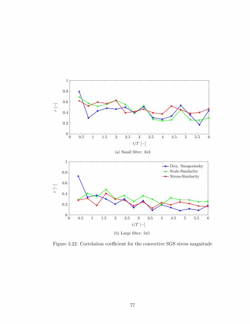
0 0.5 1 1.5 2 2.5 3 3.5 4 4.5 5 5.5 60
0.2
0.4
0.6
0.8
1
t/T [−]
r[−
]
(a) Small filter: 3x3
0 0.5 1 1.5 2 2.5 3 3.5 4 4.5 5 5.5 60
0.2
0.4
0.6
0.8
1
t/T [−]
r[−
]
Dyn. Smagorinsky
Scale-Similarity
Stress-Similarity
(b) Large filter: 5x5
Figure 3.22: Correlation coefficient for the convective SGS stress magnitude
77
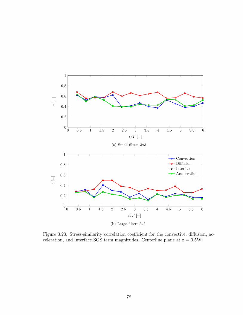
0 0.5 1 1.5 2 2.5 3 3.5 4 4.5 5 5.5 60
0.2
0.4
0.6
0.8
1
t/T [−]
r[−
]
(a) Small filter: 3x3
0 0.5 1 1.5 2 2.5 3 3.5 4 4.5 5 5.5 60
0.2
0.4
0.6
0.8
1
t/T [−]
r[−
]
Convection
Diffusion
Interface
Acceleration
(b) Large filter: 5x5
Figure 3.23: Stress-similarity correlation coefficient for the convective, diffusion, ac-celeration, and interface SGS term magnitudes. Centerline plane at z = 0.5W.
78

the formation of complex interfacial structures. The introduction of these structures
complicates the spatial variation of the fluid properties that are used in the dynamic
coefficient calculation of the eddy-viscosity model. The dynamic procedure breaks
down because of the built-in assumption of small variations between the grid and test
levels. During the most important stages of wave breaking (0.4 < t/T < 2.4), the
similarity-based models give an average correlation coefficient of approximately 0.55.
The correlation coefficients calculated using the data filtered with the 5x5x5 stencil
are reduced compared to the small-filter results just as in the phase-inversion problem.
The three tested models behave similarity throughout the simulated time period
and the correlation coefficients are reduced by approximately 50% compared to the
small filter results. The same trend is observed in Figure 3.23 where the correlation
coefficients for the convective, diffusive, acceleration, and interfacial SGS terms are
shown. The interface and acceleration terms have the same correlation coefficients
due to the coupling between the density and volume fraction fields (see Section 3.2.2
for details). The diffusive term shows the best correlation for both filter sizes with a
time-average value of approximately r = 0.6. The performance of the stress-similarity
model for the other subgrid terms is somewhat worse with a time-average of r ≈ 0.5
using the small filter. The model’s performance is degraded by approximately 30 to
50% by the use of the larger filter in the a priori analysis.
The reduction in the correlation is investigated in more detail by examining the
magnitudes of the true subgrid interfacial behavior |τI | and the modeled contribution
|τI∗| based on the stress-similarity formulation. The same three instances in time
(before and after impact, and approaching steady-state) are selected and the contours
of the terms obtained using the small filter are shown in Figure 3.24 on the center-
plane of the domain.
Before the overturning jet makes contact with the wave’s front face, the magni-
tude of the modeled-subgrid term is approximately two to three times greater than
79
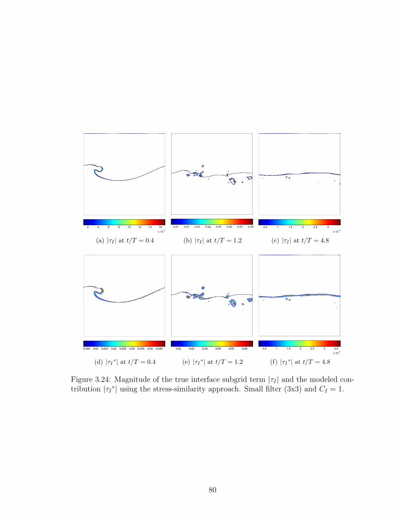
2 4 6 8 10 12 14 16
x 10−3
(a) |τI | at t/T = 0.4
0.01 0.02 0.03 0.04 0.05 0.06 0.07 0.08
(b) |τI | at t/T = 1.2
0.5 1 1.5 2 2.5 3
x 10−3
(c) |τI | at t/T = 4.8
0.005 0.01 0.015 0.02 0.025 0.03 0.035 0.04 0.045
(d) |τI∗| at t/T = 0.4
0.01 0.02 0.03 0.04 0.05 0.06
(e) |τI∗| at t/T = 1.2
0.5 1 1.5 2 2.5 3 3.5
x 10−3
(f) |τI∗| at t/T = 4.8
Figure 3.24: Magnitude of the true interface subgrid term |τI | and the modeled con-tribution |τI∗| using the stress-similarity approach. Small filter (3x3) and CI = 1.
80

0.005 0.01 0.015 0.02 0.025 0.03 0.035 0.04 0.045
(a) |τI | at t/T = 0.4
0.01 0.02 0.03 0.04 0.05 0.06 0.07 0.08
(b) |τI | at t/T = 1.2
0.5 1 1.5 2 2.5 3 3.5 4 4.5
x 10−3
(c) |τI | at t/T = 4.8
0.01 0.02 0.03 0.04 0.05 0.06 0.07 0.08 0.09 0.1
(d) |τI∗| at t/T = 0.4
0.01 0.02 0.03 0.04 0.05 0.06 0.07 0.08
(e) |τI∗| at t/T = 1.2
1 2 3 4 5 6 7 8 9 10
x 10−3
(f) |τI∗| at t/T = 4.8
Figure 3.25: Magnitude of the true interface subgrid term |τI | and the modeled con-tribution |τI∗| using the stress-similarity approach. Large filter (5x5) and CI = 1.
81

|τI |. The same trend of over-estimating the subgrid contribution using the similar-
ity approach with two different filter-cutoffs was found in the phase-inversion study,
especially in the early stages of the flow development. The spatial distribution of
the peak subgrid contribution is reproduced by the model at t/T = 0.4, but with
greater spreading across the interface region due to the size of the test-filter sten-
cil. The modeled term is found to match the magnitude of the true subgrid term at
t/T = 1.2. At this point, the jet has already impacted the front face of the wave and
several air cavities are entrained below the free surface. Addtionally, water droplets
of various sizes are propelled into the air with large horizontal velocities. The model
for the subgrid interfacial term is found to be highly active near the splash-up region
and in the proximity of the entrained air cavities. The influence of the model extends
beyond the region where the true subgrid term is confined to, resulting in the relative
low correlation coefficients shown in Figure 3.23(a).
The correlation of the stress-similarity models was found to degrade further with
the use of the larger stencil. This behavior is explained by the contours of the modeled
interfacial SGS contribution shown in Figure 3.25. The large test-filter-cutoff length-
scale spreads the influence of the model over a much greater region compared to the
true subgrid term. The size of the test filter is selected to be twice the size of the grid
filter based on the findings of previous a priori studies of various canonical turbulent
flows. However, the results presented here indicate that the ratio of the test-to-grid
filter needs to be examined in greater detail for interfacial flows where the turbulent
structures of interest are confined to the regions proximal to the fluid interface.
3.4 Summary
This chapter presents the highly-resolved simulations of two canonical turbulent-
interfacial flows and the a priori analysis of the subgrid-scale terms. The method
82

of quantifying the subgrid contributions is validated against published results of a
fully-developed turbulent channel flow and the phase-inversion problem. Then, the
subgrid terms are analyzed for the problem of a three-dimensional plunging-breaking
wave. The relative maximum contributions of the convective and the interfacial SGS
terms are on the order of the resolved counterparts during the most energetic stages of
the wave breaking process. Several modeling techniques of the subgrid-scale behavior
are examined by comparing the true subgrid terms versus the output of the models.
The structural type of SGS modeling is found to be highly correlated with the true
subgrid stresses, but the correlation coefficients tend to be strongly affected by the
size of the grid and test-level filters.
83

CHAPTER 4
Large-Eddy Simulations of Turbulent
Interfacial Marine Flows
In this chapter, important turbulent-interfacial flows are studied with large-eddy sim-
ulations. The stress-similarity-based model for the multiphase SGS terms is imple-
mented into the LES solver. The phase inversion and the plunging-breaking wave
problems are studied a posteriori to understand the role of the SGS terms in prac-
tice. The results from the a priori study are used as a basis for the selection the
SGS terms that are modeled. Furthermore, the problem of steep and breaking waves
impinging on a circular cylinder piercing the air-water interface is studied. The in-line
force on the cylinder and the prediction of the free-surface elevation in the proximity
of the structure are examined using several subgrid-scale modeling approaches.
The a priori findings from Chapter 3 require further examination through the a
posteriori study using actual large-eddy simulations with implemented closure mod-
els. The correlation coefficients for various subgrid-scale stress models obtained a
priori have been shown to not necessarily indicate the quality of the LES results
(Park et al. (2005)). In fact, high correlation between the true subgrid-scale stress
calculated from DNS data and the modeled subgrid-scale stress may not be sufficient
to guarantee the model’s performance in actual large-eddy simulations. Furthermore,
the a priori analyses compare the maxima of the subgrid terms that are found to
vary significantly in magnitude as a function of space and time and thus the conclu-
84

sions drawn from the a priori study may not translate directly to practical large-eddy
simulations.
Several flow quantities including kinetic energy and its dissipation rate are com-
puted from the large-eddy simulations and compared to the direct numerical simula-
tions results where possible. Experimental data is used for validation for the cylinder
in waves problem. The performance of the selected closure models applied to the
simulation of the three interfacial flows is then summarized.
4.1 Modeling Multiphase Subgrid Contributions
The stress-similarity model is selected to approximate the subgrid behavior of the
interfacial, acceleration, and diffusive SGS terms defined in Section 2.3.1. The model
selection is justified through the a priori study and also based on published studies
that utilize the stress-similarity concept to model non-traditional LES terms such
as the subgrid scalar transport (Chumakov (2005)). The convective SGS stress is
modeled using the dynamic Smagorinsky model and the mixed model of Zang et al.
(1993) as implemented by the University of Rostock LeMoS research group (see for
example Kornev et al. (2006)). The details of the convective models are discussed in
Section 2.2.2.
The SGS terms associated with the presence of the fluid interface are modeled as
follows:
τI∗i = CI
(ui α− ui α
), (4.1)
τA∗i = CA
(ρ ui − ρ ui
), (4.2)
τD∗ij = CD
(M −N
), (4.3)
where
M = µ
(∂ui∂xj
+∂uj∂xi
)(4.4)
85
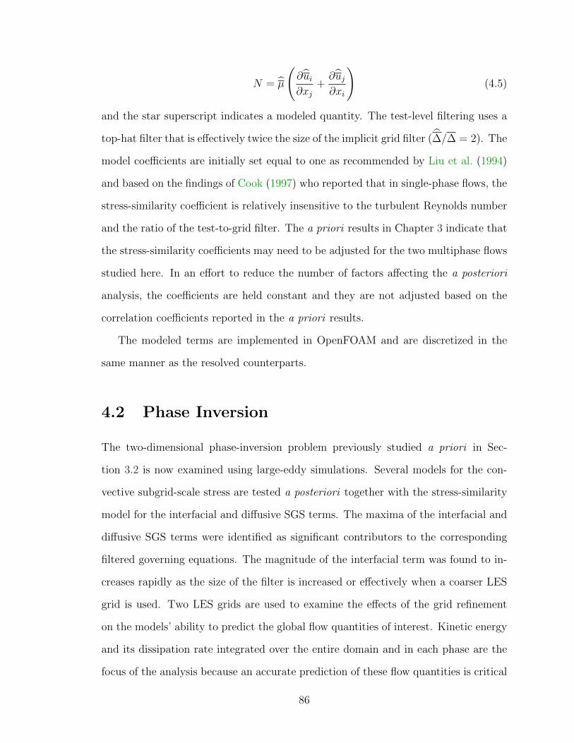
N = µ
(∂ui∂xj
+∂uj∂xi
)(4.5)
and the star superscript indicates a modeled quantity. The test-level filtering uses a
top-hat filter that is effectively twice the size of the implicit grid filter (∆/∆ = 2). The
model coefficients are initially set equal to one as recommended by Liu et al. (1994)
and based on the findings of Cook (1997) who reported that in single-phase flows, the
stress-similarity coefficient is relatively insensitive to the turbulent Reynolds number
and the ratio of the test-to-grid filter. The a priori results in Chapter 3 indicate that
the stress-similarity coefficients may need to be adjusted for the two multiphase flows
studied here. In an effort to reduce the number of factors affecting the a posteriori
analysis, the coefficients are held constant and they are not adjusted based on the
correlation coefficients reported in the a priori results.
The modeled terms are implemented in OpenFOAM and are discretized in the
same manner as the resolved counterparts.
4.2 Phase Inversion
The two-dimensional phase-inversion problem previously studied a priori in Sec-
tion 3.2 is now examined using large-eddy simulations. Several models for the con-
vective subgrid-scale stress are tested a posteriori together with the stress-similarity
model for the interfacial and diffusive SGS terms. The maxima of the interfacial and
diffusive SGS terms were identified as significant contributors to the corresponding
filtered governing equations. The magnitude of the interfacial term was found to in-
creases rapidly as the size of the filter is increased or effectively when a coarser LES
grid is used. Two LES grids are used to examine the effects of the grid refinement
on the models’ ability to predict the global flow quantities of interest. Kinetic energy
and its dissipation rate integrated over the entire domain and in each phase are the
focus of the analysis because an accurate prediction of these flow quantities is critical
86
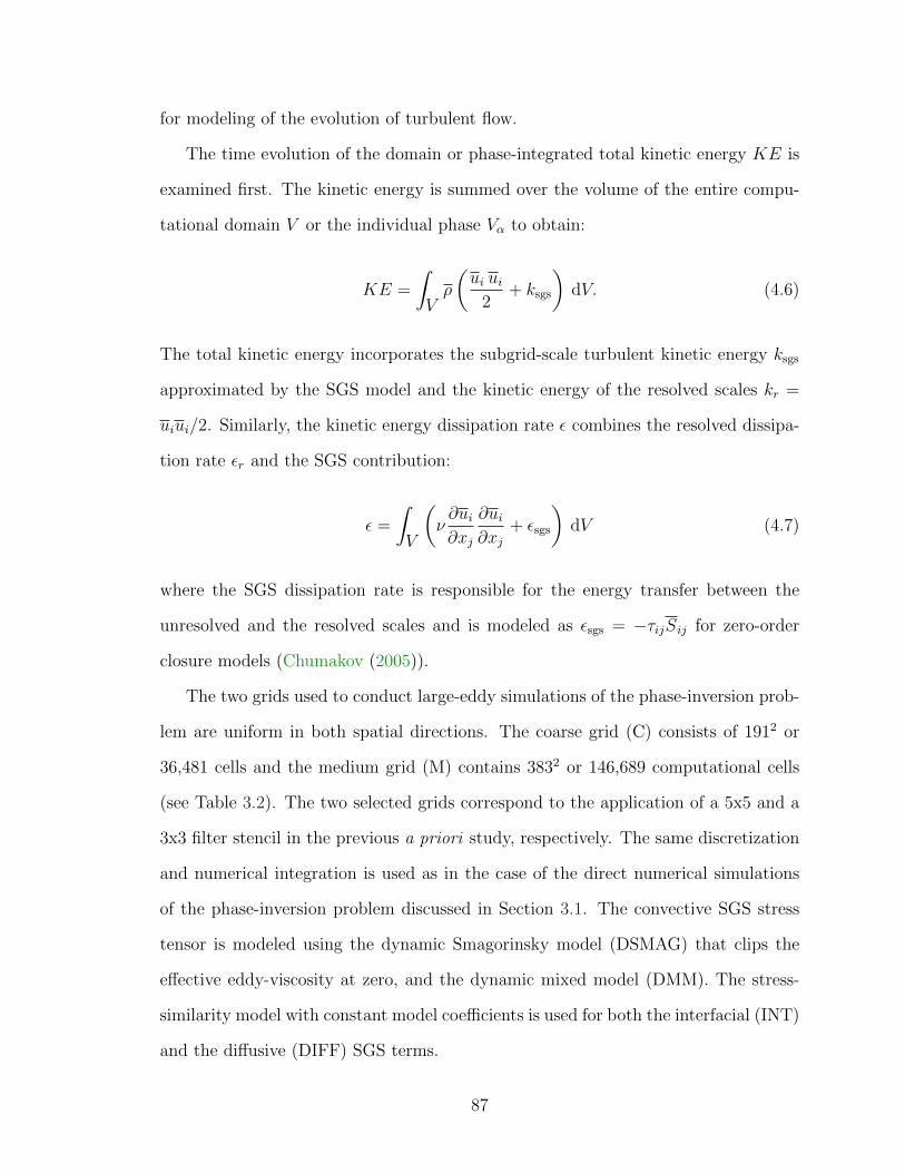
for modeling of the evolution of turbulent flow.
The time evolution of the domain or phase-integrated total kinetic energy KE is
examined first. The kinetic energy is summed over the volume of the entire compu-
tational domain V or the individual phase Vα to obtain:
KE =
∫Vρ
(ui ui
2+ ksgs
)dV. (4.6)
The total kinetic energy incorporates the subgrid-scale turbulent kinetic energy ksgs
approximated by the SGS model and the kinetic energy of the resolved scales kr =
uiui/2. Similarly, the kinetic energy dissipation rate ε combines the resolved dissipa-
tion rate εr and the SGS contribution:
ε =
∫V
(ν∂ui∂xj
∂ui∂xj
+ εsgs
)dV (4.7)
where the SGS dissipation rate is responsible for the energy transfer between the
unresolved and the resolved scales and is modeled as εsgs = −τijSij for zero-order
closure models (Chumakov (2005)).
The two grids used to conduct large-eddy simulations of the phase-inversion prob-
lem are uniform in both spatial directions. The coarse grid (C) consists of 1912 or
36,481 cells and the medium grid (M) contains 3832 or 146,689 computational cells
(see Table 3.2). The two selected grids correspond to the application of a 5x5 and a
3x3 filter stencil in the previous a priori study, respectively. The same discretization
and numerical integration is used as in the case of the direct numerical simulations
of the phase-inversion problem discussed in Section 3.1. The convective SGS stress
tensor is modeled using the dynamic Smagorinsky model (DSMAG) that clips the
effective eddy-viscosity at zero, and the dynamic mixed model (DMM). The stress-
similarity model with constant model coefficients is used for both the interfacial (INT)
and the diffusive (DIFF) SGS terms.
87
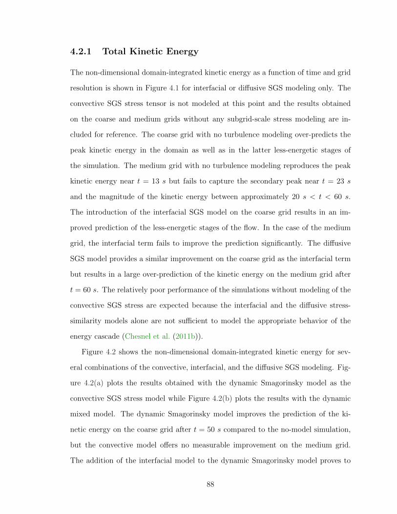
4.2.1 Total Kinetic Energy
The non-dimensional domain-integrated kinetic energy as a function of time and grid
resolution is shown in Figure 4.1 for interfacial or diffusive SGS modeling only. The
convective SGS stress tensor is not modeled at this point and the results obtained
on the coarse and medium grids without any subgrid-scale stress modeling are in-
cluded for reference. The coarse grid with no turbulence modeling over-predicts the
peak kinetic energy in the domain as well as in the latter less-energetic stages of
the simulation. The medium grid with no turbulence modeling reproduces the peak
kinetic energy near t = 13 s but fails to capture the secondary peak near t = 23 s
and the magnitude of the kinetic energy between approximately 20 s < t < 60 s.
The introduction of the interfacial SGS model on the coarse grid results in an im-
proved prediction of the less-energetic stages of the flow. In the case of the medium
grid, the interfacial term fails to improve the prediction significantly. The diffusive
SGS model provides a similar improvement on the coarse grid as the interfacial term
but results in a large over-prediction of the kinetic energy on the medium grid after
t = 60 s. The relatively poor performance of the simulations without modeling of the
convective SGS stress are expected because the interfacial and the diffusive stress-
similarity models alone are not sufficient to model the appropriate behavior of the
energy cascade (Chesnel et al. (2011b)).
Figure 4.2 shows the non-dimensional domain-integrated kinetic energy for sev-
eral combinations of the convective, interfacial, and the diffusive SGS modeling. Fig-
ure 4.2(a) plots the results obtained with the dynamic Smagorinsky model as the
convective SGS stress model while Figure 4.2(b) plots the results with the dynamic
mixed model. The dynamic Smagorinsky model improves the prediction of the ki-
netic energy on the coarse grid after t = 50 s compared to the no-model simulation,
but the convective model offers no measurable improvement on the medium grid.
The addition of the interfacial model to the dynamic Smagorinsky model proves to
88
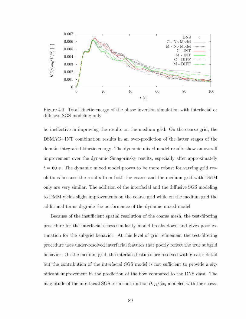
0
0.001
0.002
0.003
0.004
0.005
0.006
0.007
0 20 40 60 80 100
KE/(ρu02V/2)
[−]
t [s]
DNSC - No ModelM - No Model
C - INTM - INT
C - DIFFM - DIFF
Figure 4.1: Total kinetic energy of the phase inversion simulation with interfacial ordiffusive SGS modeling only
be ineffective in improving the results on the medium grid. On the coarse grid, the
DSMAG+INT combination results in an over-prediction of the latter stages of the
domain-integrated kinetic energy. The dynamic mixed model results show an overall
improvement over the dynamic Smagorinsky results, especially after approximately
t = 60 s. The dynamic mixed model proves to be more robust for varying grid res-
olutions because the results from both the coarse and the medium grid with DMM
only are very similar. The addition of the interfacial and the diffusive SGS modeling
to DMM yields slight improvements on the coarse grid while on the medium grid the
additional terms degrade the performance of the dynamic mixed model.
Because of the insufficient spatial resolution of the coarse mesh, the test-filtering
procedure for the interfacial stress-similarity model breaks down and gives poor es-
timation for the subgrid behavior. At this level of grid refinement the test-filtering
procedure uses under-resolved interfacial features that poorly reflect the true subgrid
behavior. On the medium grid, the interface features are resolved with greater detail
but the contribution of the interfacial SGS model is not sufficient to provide a sig-
nificant improvement in the prediction of the flow compared to the DNS data. The
magnitude of the interfacial SGS term contribution ∂τI i/∂xi modeled with the stress-
89
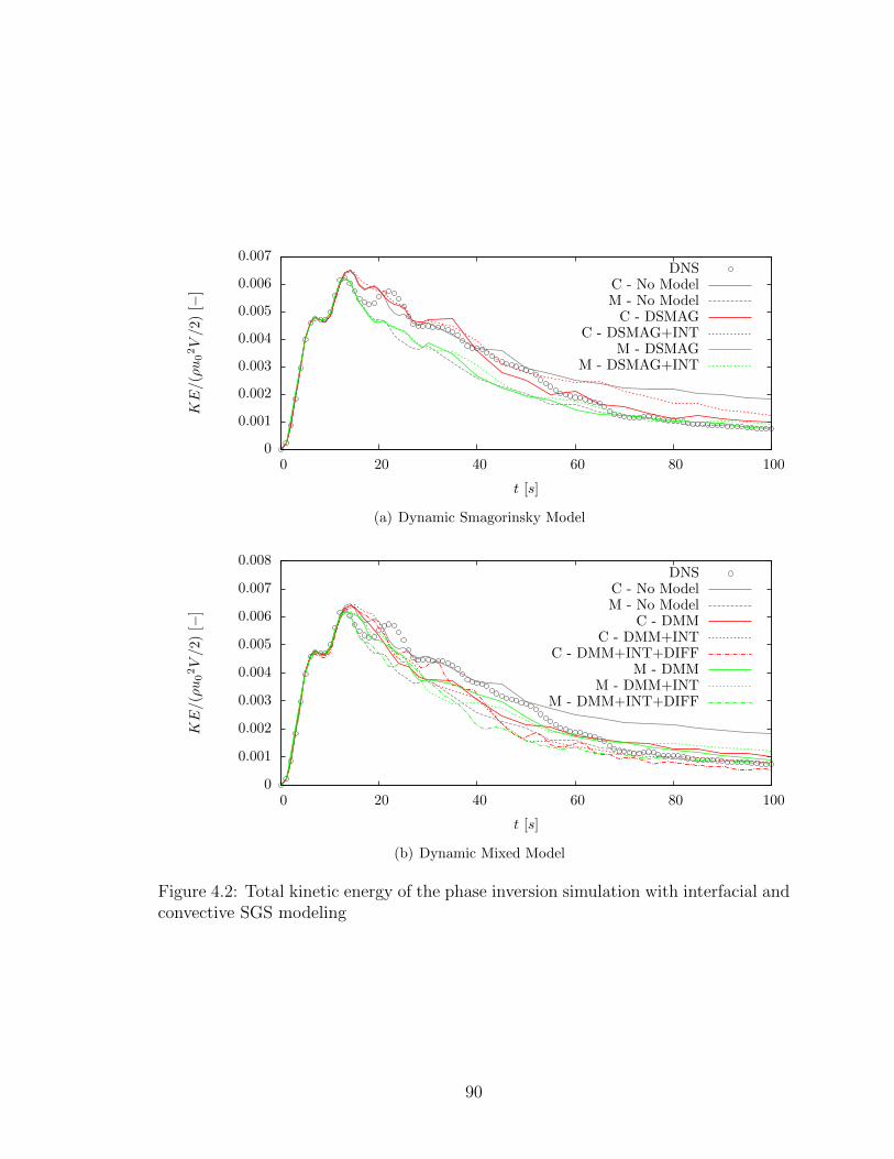
0
0.001
0.002
0.003
0.004
0.005
0.006
0.007
0 20 40 60 80 100
KE/(ρu02V/2)
[−]
t [s]
DNSC - No ModelM - No Model
C - DSMAGC - DSMAG+INT
M - DSMAGM - DSMAG+INT
(a) Dynamic Smagorinsky Model
0
0.001
0.002
0.003
0.004
0.005
0.006
0.007
0.008
0 20 40 60 80 100
KE/(ρu02V/2)
[−]
t [s]
DNSC - No ModelM - No Model
C - DMMC - DMM+INT
C - DMM+INT+DIFFM - DMM
M - DMM+INTM - DMM+INT+DIFF
(b) Dynamic Mixed Model
Figure 4.2: Total kinetic energy of the phase inversion simulation with interfacial andconvective SGS modeling
90
similarity concept is shown in Figure 4.3 on both LES grids. The model’s contribution
on the medium grid reaches 1% of the resolved term in small localized regions of the
interface. This behavior was found in the a priori study and is also verified through
the a posteriori analysis. A dynamic adjustment of the stress-similarity coefficient
for the interfacial subgrid-scale model appears to be necessary in order to improve
the model’s performance on sufficiently-resolved LES grids.
Figure 4.4 depicts the kinetic energy integrated over only the water phase or
where 0.99 ≤ α ≤ 1 and without the interfacial SGS modeling. The influence of
interface on the performance of the selected SGS models is partially removed in
this analysis to study the models’ performance away from the turbulent water-oil
interface. The dynamic Smagorinsky model results on the coarse grid match the
DNS data for the majority of the simulation but the model is unable to correctly
predict the most energetic stage of the flow development between 15 s < t < 20 s.
The results from the medium grid during the same time interval show a slight under-
prediction of the kinetic energy in water followed by a significant under-prediction
between 20 s < t < 55 s. The results using the dynamic mixed model by itself and
combined with the diffusive SGS model are shown in Figure 4.4(b). The mixed model
is again found to be more robust for different grid resolutions compared to the dynamic
Smagorinsky model because of the addition of the scale-similarity contribution which
reduces the model’s dependence on the eddy-viscosity component. The medium grid
results are improved over the DSMAG simulations while the addition of the diffusive
model to DMM on the coarse grid yields an improvement in prediction of KE in
water between 20 s < t < 35 s.
4.2.2 Kinetic Energy Dissipation Rate
The selected models are now examined for their ability to simulate the correct energy
transfer process between the resolved and subgrid scales by examining the kinetic
91

(a) M - DMM+INT
(b) C - DMM+INT
Figure 4.3: Maximum resolved component of the interface equation and the corre-sponding interfacial stress-similarity model contribution at t = 17 s
92
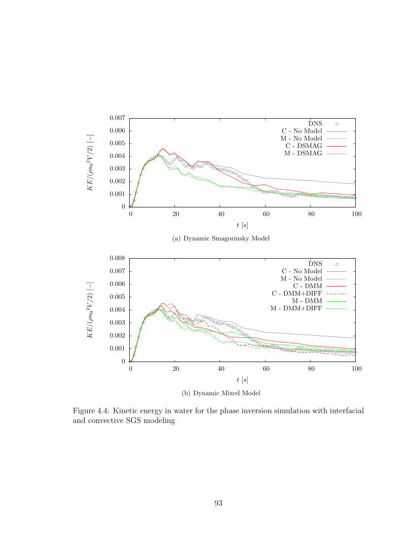
0
0.001
0.002
0.003
0.004
0.005
0.006
0.007
0 20 40 60 80 100
KE/(ρu02V/2)
[−]
t [s]
DNSC - No ModelM - No Model
C - DSMAGM - DSMAG
(a) Dynamic Smagorinsky Model
0
0.001
0.002
0.003
0.004
0.005
0.006
0.007
0.008
0 20 40 60 80 100
KE/(ρu02V/2)
[−]
t [s]
DNSC - No ModelM - No Model
C - DMMC - DMM+DIFF
M - DMMM - DMM+DIFF
(b) Dynamic Mixed Model
Figure 4.4: Kinetic energy in water for the phase inversion simulation with interfacialand convective SGS modeling
93

energy dissipation rate integrated over the computational domain.
Figure 4.5 shows the results for interfacial and diffusive SGS modeling only without
consideration for the convective term. In these simulations, the emphasis is placed on
the resolved kinetic energy dissipation rate because of the lack of an eddy-viscosity
model responsible for the subgrid dissipation. The first peak in the dissipation rate
near t = 7 s is accurately reproduced in all simulations because at this time the flow
is mostly laminar and the interface is relatively undisturbed. The global maximum
is correctly predicted in magnitude on both grids, but its time of occurrence matches
the DNS results only on the medium grid using the diffusive SGS stress-similarity
model. The increase in the dissipation rate between 55 s < t < 70 s is not captured
on either grid.
0
0.0002
0.0004
0.0006
0.0008
0.001
0.0012
0 20 40 60 80 100
ε/(u
03/λ
)[−
]
t [s]
DNSC - No ModelM - No Model
C - INTM - INT
C - DIFFM - DIFF
Figure 4.5: Kinetic energy dissipation rate for the phase inversion simulation withinterfacial or diffusive SGS modeling only
The results with the convective SGS models are shown in Figure 4.6. The dynamic
mixed model results on the medium grid correctly predict the time and magnitude
of the peak dissipation rate occurrence, whereas the maximum occurs too early on
the coarse grid and the addition of interfacial or diffusive SGS modeling does not im-
prove the result. The differences between the coarse and medium grids using DMM
are smaller than for DSMAG, but between 20 s < t < 40 s the dynamic Smagorinsky
94

model on the medium grid gives the best prediction of the domain-integrated dissipa-
tion rate. The various combinations of the convective, interfacial, and diffusive SGS
modeling do not offer a significant improvement over just modeling of the convective
subgrid-scale stress tensor. These results are similar to the analysis of the kinetic
energy results shown previously.
0
0.0002
0.0004
0.0006
0.0008
0.001
0.0012
0 20 40 60 80 100
ε/(u
03/λ
)[−
]
t [s]
DNSC - No ModelM - No Model
C - DSMAGC - DSMAG+INT
M - DSMAGM - DSMAG+INT
(a) Dynamic Smagorinsky Model
0
0.0002
0.0004
0.0006
0.0008
0.001
0.0012
0.0014
0 20 40 60 80 100
ε/(u
03/λ
)[−
]
t [s]
DNSC - No ModelM - No Model
C - DMMC - DMM+INT
C - DMM+INT+DIFFM - DMM
M - DMM+INTM - DMM+INT+DIFF
(b) Dynamic Mixed Model
Figure 4.6: Kinetic energy dissipation rate for the phase inversion simulation withinterfacial, diffusive, and convective SGS modeling
The fully-resolved direct numerical simulation results for the maximum dissipation
rate at t = 17 s are shown in Figure 4.7(a). Local dissipation rate maxima are found
95
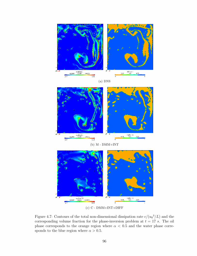
(a) DNS
(b) M - DMM+INT
(c) C - DMM+INT+DIFF
Figure 4.7: Contours of the total non-dimensional dissipation rate ε/(u03/L) and the
corresponding volume fraction for the phase-inversion problem at t = 17 s. The oilphase corresponds to the orange region where α < 0.5 and the water phase corre-sponds to the blue region where α > 0.5.
96
near the left and top walls where the oil is present and at the oil-water interface where
large velocity gradients are found. In order for the large-eddy simulations to correctly
model these regions there must be an appropriate balance between the resolved and
subgrid-scale contributions. The best LES results for the kinetic energy dissipation
rate are found using the medium grid and the dynamic mixed model combined with
the interfacial SGS model (shown in Figure 4.7(b)), while the worst LES results are
found using the coarse grid and with the DMM+INT+DIFF combination (shown in
Figure 4.7(c)). The reduction of resolved-flow detail such as the long oil filaments
is clearly shown on the coarse LES grid and to a lesser extent on the medium grid.
The dynamic mixed model combined with the interfacial stress-similarity model on
the medium grid reproduces the the large-local dissipation rates near the walls and
in some regions of the water-oil interface. The results on the coarse grid significantly
under-predict these flow characteristics and hence the domain-integrated dissipation
rate is also under predicted.
4.3 Plunging-Breaking Wave
The a posteriori study of the LES models is now extended to the three-dimensional
problem of a plunging-breaking water wave previously studied with direct-numerical
simulations in Section 3.3. The diffusive and the interfacial SGS terms were identified
as relatively important contributors to the filtered governing equations, similar to the
findings in the phase-inversion problem. The acceleration term was found to be
larger for the plunging-breaking wave compared to the phase-inversion problem, but
this SGS term is not examined here. The acceleration SGS term is found to be more
than an order of magnitude smaller relative to the other SGS terms and hence it is
not modeled to bound the scope of the study.
Domain-integrated quantities including the kinetic energy and the kinetic energy
97
dissipation rate are investigated on a relatively coarse numerical grid compared to
the DNS resolution. The LES domain has the same physical dimensions as the DNS
grid (see Figure 3.13) and is discretized with 128 cells in the streamwise and vertical
direction (Nx = Ny = 128) and 64 cells in the spanwise direction (Nz = 64), giving
a uniformly-spaced numerical grid with 1,048,576 computational cells. The selected
grid corresponds to the application of a 5x5x5 filter stencil in the a priori study.
The spanwise and streamwise boundaries are periodic while the top and bottom are
considered as no-slip boundaries. The initial wave profile and water particle velocities
are initialized in the same manner as in the a priori study using Stokes third-order
theory. The same discretization and numerical integration schemes are used as in the
case of direct numerical simulations.
The dynamic mixed model is tested individually and also combined with the stress-
similarity model with constant coefficients for the diffusive and the interfacial subgrid-
scale terms. The dynamic Smagorinsky model is combined with the interfacial SGS
model based on the results found in the phase inversion simulations. A pure stress-
similarity model combining the diffusive and interfacial terms without any convective
SGS modeling is also examined.
4.3.1 Kinetic Energy and Energy Dissipation
The kinetic energy and its dissipation rate integrated over the computational domain
are calculated using Equations 4.6 and 4.7. The non-dimensionalized results are
summarized in Figure 4.8 for the first two wave periods. During this time period the
flow changes rapidly as the initial wave profile breaks in a plunging event and thus the
largest magnitudes of the kinetic energy and its dissipation rate are recorded. The
ability of the LES model to predict the most energetic stages of the flow evolution is
important because in the case of wave impacts on offshore structures, the occurrence
of the largest excitation forces is typically correlated with the high-energy events.
98
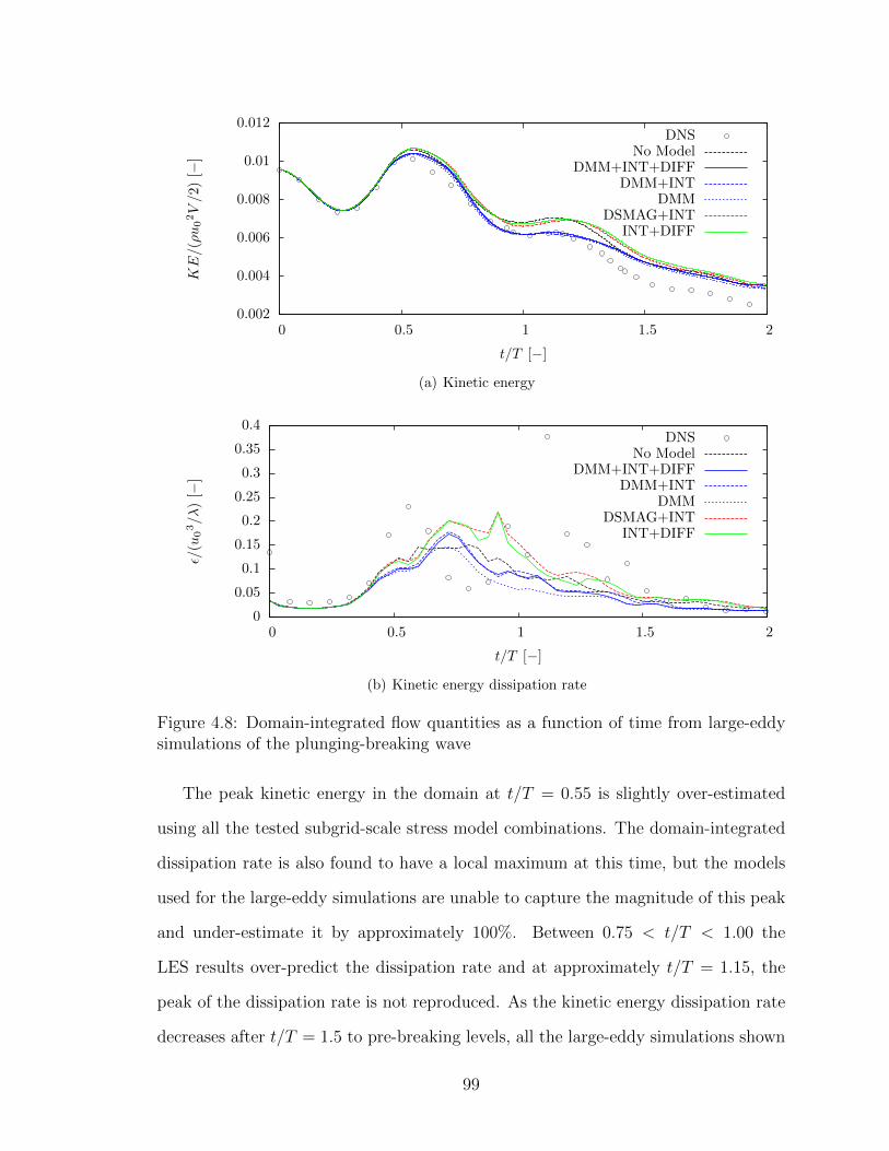
0.002
0.004
0.006
0.008
0.01
0.012
0 0.5 1 1.5 2
KE/(ρu02V/2)
[−]
t/T [−]
DNSNo Model
DMM+INT+DIFFDMM+INT
DMMDSMAG+INT
INT+DIFF
(a) Kinetic energy
0
0.05
0.1
0.15
0.2
0.25
0.3
0.35
0.4
0 0.5 1 1.5 2
ε/(u
03/λ
)[−
]
t/T [−]
DNSNo Model
DMM+INT+DIFFDMM+INT
DMMDSMAG+INT
INT+DIFF
(b) Kinetic energy dissipation rate
Figure 4.8: Domain-integrated flow quantities as a function of time from large-eddysimulations of the plunging-breaking wave
The peak kinetic energy in the domain at t/T = 0.55 is slightly over-estimated
using all the tested subgrid-scale stress model combinations. The domain-integrated
dissipation rate is also found to have a local maximum at this time, but the models
used for the large-eddy simulations are unable to capture the magnitude of this peak
and under-estimate it by approximately 100%. Between 0.75 < t/T < 1.00 the
LES results over-predict the dissipation rate and at approximately t/T = 1.15, the
peak of the dissipation rate is not reproduced. As the kinetic energy dissipation rate
decreases after t/T = 1.5 to pre-breaking levels, all the large-eddy simulations shown
99
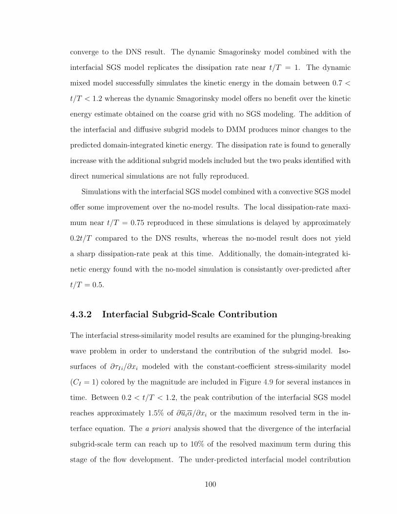
converge to the DNS result. The dynamic Smagorinsky model combined with the
interfacial SGS model replicates the dissipation rate near t/T = 1. The dynamic
mixed model successfully simulates the kinetic energy in the domain between 0.7 <
t/T < 1.2 whereas the dynamic Smagorinsky model offers no benefit over the kinetic
energy estimate obtained on the coarse grid with no SGS modeling. The addition of
the interfacial and diffusive subgrid models to DMM produces minor changes to the
predicted domain-integrated kinetic energy. The dissipation rate is found to generally
increase with the additional subgrid models included but the two peaks identified with
direct numerical simulations are not fully reproduced.
Simulations with the interfacial SGS model combined with a convective SGS model
offer some improvement over the no-model results. The local dissipation-rate maxi-
mum near t/T = 0.75 reproduced in these simulations is delayed by approximately
0.2t/T compared to the DNS results, whereas the no-model result does not yield
a sharp dissipation-rate peak at this time. Additionally, the domain-integrated ki-
netic energy found with the no-model simulation is consistantly over-predicted after
t/T = 0.5.
4.3.2 Interfacial Subgrid-Scale Contribution
The interfacial stress-similarity model results are examined for the plunging-breaking
wave problem in order to understand the contribution of the subgrid model. Iso-
surfaces of ∂τI i/∂xi modeled with the constant-coefficient stress-similarity model
(CI = 1) colored by the magnitude are included in Figure 4.9 for several instances in
time. Between 0.2 < t/T < 1.2, the peak contribution of the interfacial SGS model
reaches approximately 1.5% of ∂uiα/∂xi or the maximum resolved term in the in-
terface equation. The a priori analysis showed that the divergence of the interfacial
subgrid-scale term can reach up to 10% of the resolved maximum term during this
stage of the flow development. The under-predicted interfacial model contribution
100
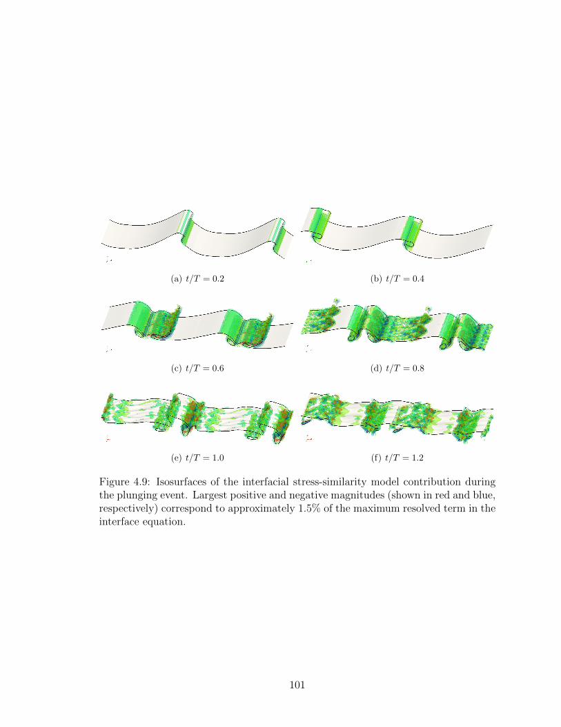
(a) t/T = 0.2 (b) t/T = 0.4
(c) t/T = 0.6 (d) t/T = 0.8
(e) t/T = 1.0 (f) t/T = 1.2
Figure 4.9: Isosurfaces of the interfacial stress-similarity model contribution duringthe plunging event. Largest positive and negative magnitudes (shown in red and blue,respectively) correspond to approximately 1.5% of the maximum resolved term in theinterface equation.
101

can be linked to the relatively low correlation coefficients of the constant-coefficient
stress-similarity model as shown in Figure 3.23(b). The correlation coefficient for the
interface term varies between approximately 0.1 < r < 0.3 throughout the simulation
time of six wave periods.
The a posteriori study of the plunging-breaking wave is conducted using a coarse
LES grid corresponding to the application of the large filter in the a priori study. Sev-
eral combinations of the dynamic mixed model and the dynamic Smagorinsky model
with the stress-similarity model for the diffusive and interfacial subgrid terms are
examined. The results for the total kinetic energy and the kinetic energy dissipation
rate indicate that the tested models are unable to correctly predict the evolution and
the temporal maxima of the dissipation rate. The dynamic mixed model is found to
perform better than the dynamic Smagorinsky model in predicting the total kinetic
energy in the domain, indicating that the inclusion of the similarity-based compo-
nent in the convective subgrid model is important for turbulent-interfacial flows. The
contribution of the constant-coefficient stress-similarity model for the interfacial SGS
term is under-predicted and thus not sufficient to significantly affect the solution.
4.4 Cylinder in Waves
The following sections focus on the simulation of breaking waves impinging on a
bottom-fixed circular cylinder piercing the free surface. An overview of the problem
setup is presented first, followed by a validation study based on experimental data.
The effects of the subgrid-scale term modeling in large-eddy simulations of breaking-
wave impacts are then investigated.
102

4.4.1 Problem Description
The force on a cylinder impinged upon by steep and/or breaking three-dimensional
waves is studied numerically. The simulation setup is based on a recent experimental
campaign summarized in Nielsen et al. (2012) and Bredmose et al. (2013). The
campaign focused on an experimental evaluation of wave loads on a vertical-circular
cylinder piercing the free surface. The experiments were conduced at the Danish DHI
wave basin in an effort to study offshore wind platforms and their survivability in
various seastates and especially when steep waves are present.
The monopile platform was fixed to a sloping bottom (slope of 1/25) and secured
in place by load cells. A system of wave probes was used to capture the free-surface
elevation at several locations close to the wave maker and the cylinder (see Fig-
ure 4.10(b)). The model-scale cylinder diameter D was 0.075 m or 6.0 m in full scale.
In the results presented here the calm-water depth at the location of the cylinder is
0.78 m in model scale. Both small-amplitude linear regular waves and high-steepness
regular waves are investigated. The length of the incoming waves is held constant
at 3.34 m in model scale and the wave period T is 1.54 s, corresponding to a wave
number k of 1.82 and intermediate water depth. The small-amplitude linear waves
have a steepness ratio H/λ = 0.030 while the steep-regular waves are initialized with
H0/λ0 = 0.084 where H0 and λ0 are the initial wave height and wave length, re-
spectively, generated at the inlet boundary or the wave maker. An initial steepness
ratio is specified because as the train of steep waves interacts with the sloping seabed
the effective steepness ratio tends to increase and the waves eventually break in the
proximity of the cylinder.
The computational domain is modeled after the experimental setup and is de-
picted in Figure 4.10. The domain width W is approximately 23D wide to minimize
the interaction of reflected waves with the side walls, the inlet length Lin is equal to λ
and the outgoing waves are damped out near the outlet boundary over Lout = 3λ. The
103
(a) Main dimensions of the computational domain
(b) Side centerline profile illustrating the 1/25 seabed slope formed between the inlet and outletboundaries and top view depicting an approximate location of the wave probes
Figure 4.10: Details of the computational domain
104
incoming waves are generated using the OpenFOAM extension toolkit waves2Foam
(Jacobsen et al. (2011)) which utilizes relaxation zones near the domain inlet and
outlet for both wave generation and damping in order to avoid unwanted wave re-
flections. This toolkit also provides the user with a large selection of wave theories
including linear waves, several orders of Stokes theory, cnoidal theory, and more. The
flow field can be initialized using any wave theory to obtain the free-surface elevation
and water particle velocities everywhere in the computational domain.
The fully-structured computational grids are constructed using the software Point-
wise. The coarse grid consists of approximately 3.6 million cells and the fine grid
contains approximately 22 million cells. At least 400 grid points per wave length and
40 grid points per wave height are used to accurately represent the free surface with
negligible numerical dissipation as shown by Piro (2013). The cylinder, seabed, and
the lateral boundaries are modeled as slip boundaries and hence they do not allow for
the development of viscous boundary layers. In the cases studied here, inertial forces
dominate the forces acting on the cylinder, but the full implications of not resolving
the viscous boundary layer formed near the body are of interest for future work. The
influence of the viscous boundary layers is anticipated to become significant when
shorter wave lengths and hence larger D/λ ratios are of interest.
The governing equations are discretized and integrated in time as in the previ-
ously discussed simulations with the exception of the convective term in the momen-
tum equation and the advection term in the interface equation. These terms are
discretized with flux-limited schemes to preserve the monotonicity of the solution
while retaining an overall second-order accuracy. Limited schemes has been shown
by Jasak (1999) to be more robust for non-uniform grids, which are common in indus-
trial simulations because of the complexity of the geometry involved. The additional
numerical dissipation that is introduced by such schemes can adversely affect LES,
but its influence is highly dependent on the grid quality (Sagaut (2001)). The quality
105

of the grids used in this study is relatively high based on several grid quality criteria
including cell expansion ratio, skewness, and non-orthogonality. Because of the high
quality grids used, the impact of the numerical dissipation associated with the limited
schemes is expected to be small.
4.4.2 Linear Regular Waves
The numerical method used to simulate water waves is first validated using small-
amplitude linear waves withH/λ = 0.030. Airy waves are generated on the coarse grid
at the domain’s inlet and propagated in the direction of the cylinder. No turbulence
modeling is used in this case because of the small wave steepness used and the lack
of complex free-surface structures. The free-surface elevation and in-line force on the
cylinder are recorded for 20 periods and compared to the experimental data. The
free-surface elevation non-dimensionalized by the wave amplitude A as a function of
time from four different wave probes is shown in Figure 4.11. Probe P1 is located on
the centerline and near the wave maker. Probe P15 is located approximately 3D in
front of the cylinder, probe P18 is located at the streamwise location of the cylinder
but offset laterally by 6D, and probe P19 is located approximately 3D downstream
of the cylinder on the centerline.
The amplitude and period of the incoming waves and the free-surface elevation
downstream from the cylinder are closely reproduced in the simulation. Minor differ-
ences in the phases are expected because of the difficulty in a perfect reproduction of
experimental data that can often contain some measurement error. The wave peaks
and troughs are consistently reproduced throughout the simulation indicating that
the choice of a limited linear scheme for the discretization of the convective term
does not result in an excessive dissipation of energy. The in-line force acting on the
cylinder is non-dimensionalized with ρgAD2 and presented in Figure 4.12. The dif-
ference between the numerical and experimental results is greater here than in the
106

-1.5
-1
-0.5
0
0.5
1
1.5
0 0.5 1 1.5 2 2.5 3 3.5 4
η/A
[−]
t [s]
ExpNum
(a) Probe 1: x = 1.00 m, y = 0.00 m
-1.5
-1
-0.5
0
0.5
1
1.5
0 0.5 1 1.5 2 2.5 3 3.5 4
η/A
[−]
t [s]
ExpNum
(b) Probe 15: x = 7.50 m, y = 0.00 m
-1.5
-1
-0.5
0
0.5
1
1.5
0 0.5 1 1.5 2 2.5 3 3.5 4
η/A
[−]
t [s]
ExpNum
(c) Probe 18: x = 7.75 m, y = −0.50 m
-1.5
-1
-0.5
0
0.5
1
1.5
0 0.5 1 1.5 2 2.5 3 3.5 4
η/A
[−]
t [s]
ExpNum
(d) Probe 19: x = 7.95 m, y = 0.00 m
Figure 4.11: Free-surface elevation of regular-linear waves at four probe locations
107
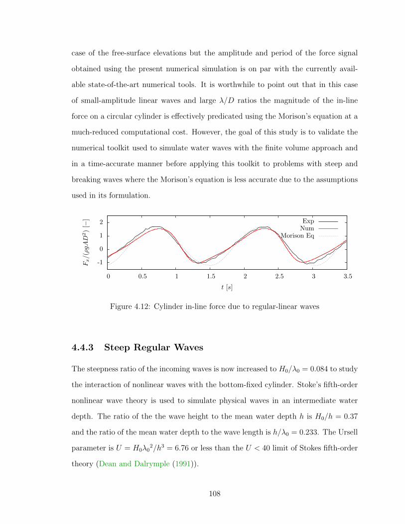
case of the free-surface elevations but the amplitude and period of the force signal
obtained using the present numerical simulation is on par with the currently avail-
able state-of-the-art numerical tools. It is worthwhile to point out that in this case
of small-amplitude linear waves and large λ/D ratios the magnitude of the in-line
force on a circular cylinder is effectively predicated using the Morison’s equation at a
much-reduced computational cost. However, the goal of this study is to validate the
numerical toolkit used to simulate water waves with the finite volume approach and
in a time-accurate manner before applying this toolkit to problems with steep and
breaking waves where the Morison’s equation is less accurate due to the assumptions
used in its formulation.
-1
0
1
2
0 0.5 1 1.5 2 2.5 3 3.5
Fx/(ρgAD
2)
[−]
t [s]
ExpNum
Morison Eq
Figure 4.12: Cylinder in-line force due to regular-linear waves
4.4.3 Steep Regular Waves
The steepness ratio of the incoming waves is now increased to H0/λ0 = 0.084 to study
the interaction of nonlinear waves with the bottom-fixed cylinder. Stoke’s fifth-order
nonlinear wave theory is used to simulate physical waves in an intermediate water
depth. The ratio of the the wave height to the mean water depth h is H0/h = 0.37
and the ratio of the mean water depth to the wave length is h/λ0 = 0.233. The Ursell
parameter is U = H0λ02/h3 = 6.76 or less than the U < 40 limit of Stokes fifth-order
theory (Dean and Dalrymple (1991)).
108

-2
0
2
4
6
0 1 2 3 4 5 6 7 8 9
Fx/( ρgA
D2) ,η/A
[−]
t [s]
ForceP18
Figure 4.13: In-line force and free-surface elevation at probe 18 (x = 7.75 m, y =−0.50 m) for steep regular wave impacts (H0/λ0 = 0.084)
The decreasing water depth due to the sloping seabed results in the incoming
waves becoming steeper and eventually breaking in either a plunging or spilling event.
A sample force and free-surface elevation time history of the steep-regular waves
impinging on the cylinder calculated on the fine grid with no turbulence modeling is
shown in Figure 4.13. The free-surface elevation is recorded at probe P18 which is
located next to the cylinder. The entire flow field at t = 0 s is initialized with the
fifth-order Stokes waves and the first wave peak is located approximately 6D in front
of the cylinder. Because this wave travels over a small portion of the sloping seabed
before impacting the cylinder, no breaking event occurs and the resulting in-line
force acting on the cylinder is considerably smaller compared to the following wave
impacts. In Figure 4.14, four instances in time between 0.2 s < t < 0.8 s illustrate the
flow-field through the free-surface elevation contour colored by the non-dimensional
amplitude (top portion of the image) and the dynamic pressure pd = p − ρgh on a
centerline plane (bottom portion of the image). The pile-up of water on the front
face of the cylinder is visible in Figure 4.14(b) followed by formation of a wake as the
wave propagates past the cylinder. The dynamic pressure field reaches its maximum
near the wake peak and remains mostly unaffected by the presence of the cylinder
109
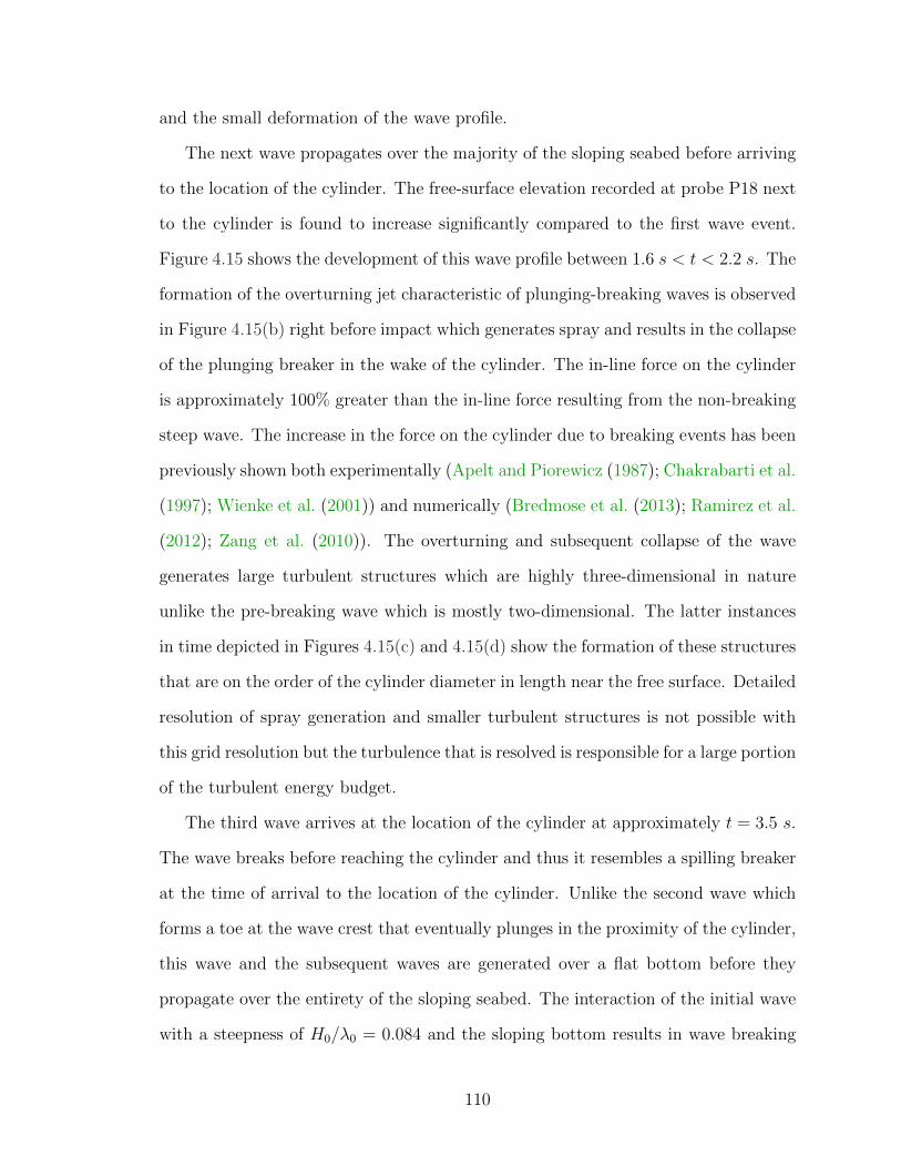
and the small deformation of the wave profile.
The next wave propagates over the majority of the sloping seabed before arriving
to the location of the cylinder. The free-surface elevation recorded at probe P18 next
to the cylinder is found to increase significantly compared to the first wave event.
Figure 4.15 shows the development of this wave profile between 1.6 s < t < 2.2 s. The
formation of the overturning jet characteristic of plunging-breaking waves is observed
in Figure 4.15(b) right before impact which generates spray and results in the collapse
of the plunging breaker in the wake of the cylinder. The in-line force on the cylinder
is approximately 100% greater than the in-line force resulting from the non-breaking
steep wave. The increase in the force on the cylinder due to breaking events has been
previously shown both experimentally (Apelt and Piorewicz (1987); Chakrabarti et al.
(1997); Wienke et al. (2001)) and numerically (Bredmose et al. (2013); Ramirez et al.
(2012); Zang et al. (2010)). The overturning and subsequent collapse of the wave
generates large turbulent structures which are highly three-dimensional in nature
unlike the pre-breaking wave which is mostly two-dimensional. The latter instances
in time depicted in Figures 4.15(c) and 4.15(d) show the formation of these structures
that are on the order of the cylinder diameter in length near the free surface. Detailed
resolution of spray generation and smaller turbulent structures is not possible with
this grid resolution but the turbulence that is resolved is responsible for a large portion
of the turbulent energy budget.
The third wave arrives at the location of the cylinder at approximately t = 3.5 s.
The wave breaks before reaching the cylinder and thus it resembles a spilling breaker
at the time of arrival to the location of the cylinder. Unlike the second wave which
forms a toe at the wave crest that eventually plunges in the proximity of the cylinder,
this wave and the subsequent waves are generated over a flat bottom before they
propagate over the entirety of the sloping seabed. The interaction of the initial wave
with a steepness of H0/λ0 = 0.084 and the sloping bottom results in wave breaking
110
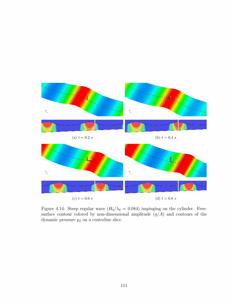
(a) t = 0.2 s (b) t = 0.4 s
(c) t = 0.6 s (d) t = 0.8 s
Figure 4.14: Steep regular wave (H0/λ0 = 0.084) impinging on the cylinder. Free-surface contour colored by non-dimensional amplitude (η/A) and contours of thedynamic pressure pd on a centerline slice.
111
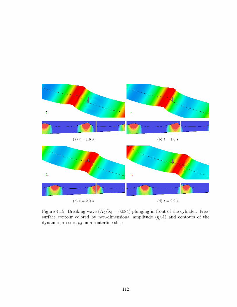
(a) t = 1.6 s (b) t = 1.8 s
(c) t = 2.0 s (d) t = 2.2 s
Figure 4.15: Breaking wave (H0/λ0 = 0.084) plunging in front of the cylinder. Free-surface contour colored by non-dimensional amplitude (η/A) and contours of thedynamic pressure pd on a centerline slice.
112
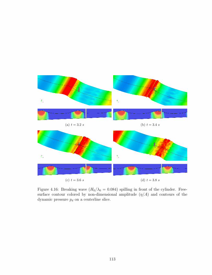
(a) t = 3.2 s (b) t = 3.4 s
(c) t = 3.6 s (d) t = 3.8 s
Figure 4.16: Breaking wave (H0/λ0 = 0.084) spilling in front of the cylinder. Free-surface contour colored by non-dimensional amplitude (η/A) and contours of thedynamic pressure pd on a centerline slice.
113
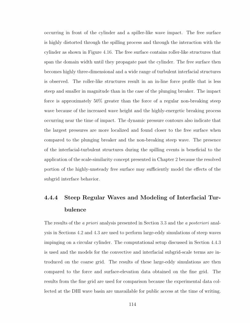
occurring in front of the cylinder and a spiller-like wave impact. The free surface
is highly distorted through the spilling process and through the interaction with the
cylinder as shown in Figure 4.16. The free surface contains roller-like structures that
span the domain width until they propagate past the cylinder. The free surface then
becomes highly three-dimensional and a wide range of turbulent interfacial structures
is observed. The roller-like structures result in an in-line force profile that is less
steep and smaller in magnitude than in the case of the plunging breaker. The impact
force is approximately 50% greater than the force of a regular non-breaking steep
wave because of the increased wave height and the highly-energetic breaking process
occurring near the time of impact. The dynamic pressure contours also indicate that
the largest pressures are more localized and found closer to the free surface when
compared to the plunging breaker and the non-breaking steep wave. The presence
of the interfacial-turbulent structures during the spilling events is beneficial to the
application of the scale-similarity concept presented in Chapter 2 because the resolved
portion of the highly-unsteady free surface may sufficiently model the effects of the
subgrid interface behavior.
4.4.4 Steep Regular Waves and Modeling of Interfacial Tur-
bulence
The results of the a priori analysis presented in Section 3.3 and the a posteriori anal-
ysis in Sections 4.2 and 4.3 are used to perform large-eddy simulations of steep waves
impinging on a circular cylinder. The computational setup discussed in Section 4.4.3
is used and the models for the convective and interfacial subgrid-scale terms are in-
troduced on the coarse grid. The results of these large-eddy simulations are then
compared to the force and surface-elevation data obtained on the fine grid. The
results from the fine grid are used for comparison because the experimental data col-
lected at the DHI wave basin are unavailable for public access at the time of writing.
114

Nonetheless, the present numerical results provide a highly-resolved dataset that is
sufficient for a preliminary evaluation of the LES models.
The a priori analysis of the phase inversion and breaking-wave problems identified
the convective term as the largest subgrid-scale terms in the studied interfacial flows.
This result is anticipated because the convective effects are responsible for a signifi-
cant portion of the energy transfer that is truncated through the application of the
low-pass filter. Additionally, previous applications of the single-phase LES concepts
to select multiphase problems have shown relative success in predicting global quanti-
ties of the flow when only modeling the convective SGS stress tensor. The interfacial
SGS term was often found to be the second largest SGS term in the breaking-wave
problem, especially at the most energetic stage of breaking. The maximum magni-
tude of the interfacial term relative to the resolved contribution can be of the same
order of magnitude as the convective term in the two interfacial flows studied. Addi-
tionally, the interfacial term is found to increase in magnitude when coarser grids or
larger filtering stencils are used and thus the interfacial SGS term is anticipated to be
important in industrial applications where coarse numerical grids are common. With
industrial applications in mind, the coarse grid described in Section 4.4.1 is used to
perform large-eddy simulations utilizing models for the convective and the interfa-
cial terms. The convective SGS stress is modeled using the robust dynamic mixed
model. The generalized scale-similarity or the stress-similarity concept described in
Section 2.3 is applied to model the interfacial SGS term.
The non-dimensional in-line force obtained on the coarse grid with and with-
out subgrid-scale modeling is compared to the highly-resolved data from the fine
grid simulation. The time series for the first six impacts is shown in Figure 4.17(a)
and a close-up of 4.5 s < t < 9.0 s is shown in Figure 4.17(b). The simulation
with the dynamic mixed model and the stress-similarity model for the interface term
(DMM+INT) is shown to give the same force profile as the other simulations between
115
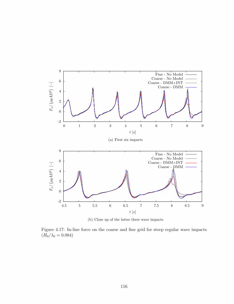
-2
0
2
4
6
8
0 1 2 3 4 5 6 7 8 9
Fx/( ρgA
D2) [−
]
t [s]
Fine - No ModelCoarse - No Model
Coarse - DMM+INTCoarse - DMM
(a) First six impacts
-2
0
2
4
6
8
4.5 5 5.5 6 6.5 7 7.5 8 8.5 9
Fx/( ρgA
D2) [−
]
t [s]
Fine - No ModelCoarse - No Model
Coarse - DMM+INTCoarse - DMM
(b) Close up of the latter three wave impacts
Figure 4.17: In-line force on the coarse and fine grid for steep regular wave impacts(H0/λ0 = 0.084)
116
0 s < t < 1 s where a steep non-breaking wave impacts the cylinder. This is expected
because the free surface does not undergo significant deformations as this time and
the contribution from the turbulence models is limited by the dynamic procedure.
Between 1.5 s < t < 4.5 s the cylinder is impinged upon by a plunging-breaking wave
and then a spilling-breaking wave, as described in Section 4.4.3. The force on the
cylinder and the timing of the arrival of the peak force due to the plunging-breaking
wave is captured well on the coarse grid. Similarly, the first spilling wave event and
the associated force is predicted well regardless of the use of the SGS modeling.
The maximum negative force on the cylinder associated with the formation of
a wake behind the cylinder is over-predicted when the SGS modeling is not used.
The free surface immediately behind the cylinder undergoes a significant deformation
due to negative pressure on the suction side of the cylinder prior to impact. At
the location of probe P19 (x = 7.95 m, y = 0.00 m or 3D downstream from the
cylinder) the free-surface elevation on the centerline shown in Figure 4.19(a) does not
differ between the two coarse grid simulations. The over-prediction of the maximum
negative force is therefore linked to the flow field in the immediate proximity of the
cylinder. Two isosurfaces of the interfacial SGS term are shown at t = 2.0 s and
t = 2.2 s in Figure 4.18. In the wake region, the stress-similarity model for the
interfacial SGS term is shown to be highly active when the peak of the wave moves
past the cylinder.
During the next three impacts between 4.5 s < t < 9.0 s the waves break in either
a weak plunging or spilling manner and the differences between the simulations on the
coarse grid become more pronounced. The flow field now retains a portion of resolved
turbulence near the cylinder once several waves propagate by and a calm condition
is no longer achievable before the arrival of the next wave. During all three impacts
the maximum negative force on the cylinder obtained using the combination of the
dynamic mixed model and the interface SGS model shows an excellent match with
117
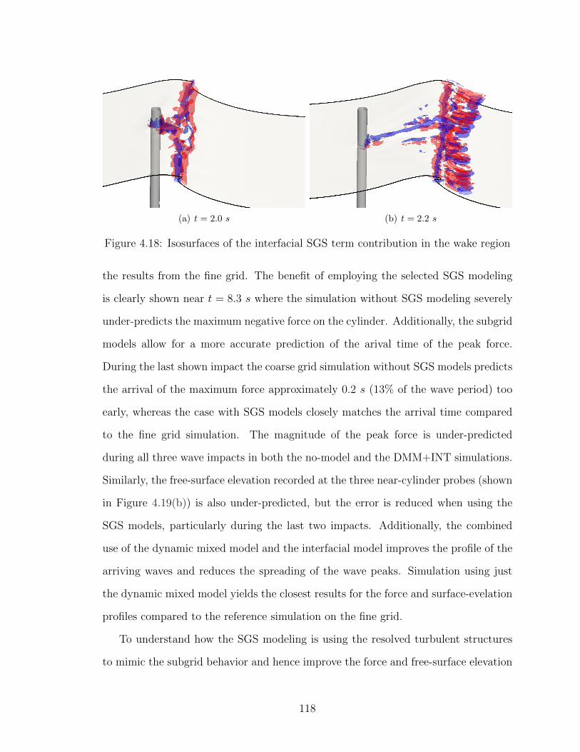
(a) t = 2.0 s (b) t = 2.2 s
Figure 4.18: Isosurfaces of the interfacial SGS term contribution in the wake region
the results from the fine grid. The benefit of employing the selected SGS modeling
is clearly shown near t = 8.3 s where the simulation without SGS modeling severely
under-predicts the maximum negative force on the cylinder. Additionally, the subgrid
models allow for a more accurate prediction of the arival time of the peak force.
During the last shown impact the coarse grid simulation without SGS models predicts
the arrival of the maximum force approximately 0.2 s (13% of the wave period) too
early, whereas the case with SGS models closely matches the arrival time compared
to the fine grid simulation. The magnitude of the peak force is under-predicted
during all three wave impacts in both the no-model and the DMM+INT simulations.
Similarly, the free-surface elevation recorded at the three near-cylinder probes (shown
in Figure 4.19(b)) is also under-predicted, but the error is reduced when using the
SGS models, particularly during the last two impacts. Additionally, the combined
use of the dynamic mixed model and the interfacial model improves the profile of the
arriving waves and reduces the spreading of the wave peaks. Simulation using just
the dynamic mixed model yields the closest results for the force and surface-evelation
profiles compared to the reference simulation on the fine grid.
To understand how the SGS modeling is using the resolved turbulent structures
to mimic the subgrid behavior and hence improve the force and free-surface elevation
118
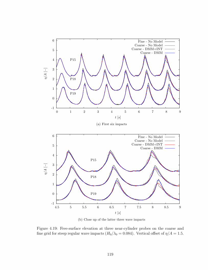
-1
0
1
2
3
4
5
6
0 1 2 3 4 5 6 7 8 9
η/A
[−]
t [s]
P15
P18
P19
Fine - No ModelCoarse - No Model
Coarse - DMM+INTCoarse - DMM
(a) First six impacts
-1
0
1
2
3
4
5
6
4.5 5 5.5 6 6.5 7 7.5 8 8.5 9
η/A
[−]
t [s]
P15
P18
P19
Fine - No ModelCoarse - No Model
Coarse - DMM+INTCoarse - DMM
(b) Close up of the latter three wave impacts
Figure 4.19: Free-surface elevation at three near-cylinder probes on the coarse andfine grid for steep regular wave impacts (H0/λ0 = 0.084). Vertical offset of η/A = 1.5.
119
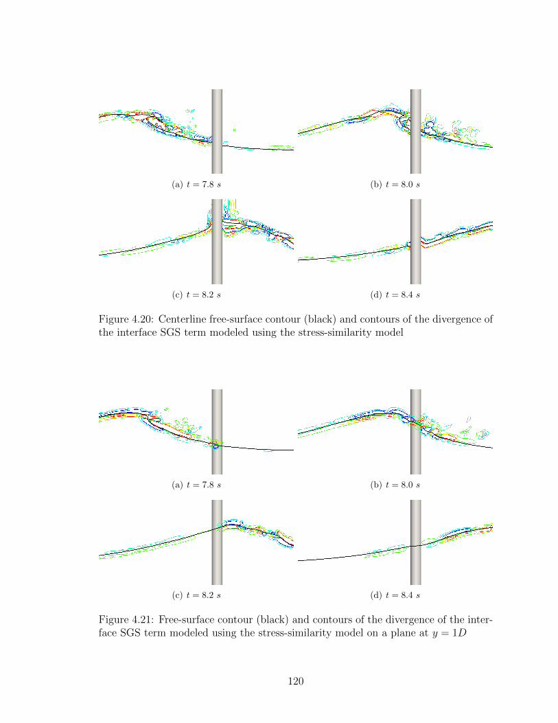
(a) t = 7.8 s (b) t = 8.0 s
(c) t = 8.2 s (d) t = 8.4 s
Figure 4.20: Centerline free-surface contour (black) and contours of the divergence ofthe interface SGS term modeled using the stress-similarity model
(a) t = 7.8 s (b) t = 8.0 s
(c) t = 8.2 s (d) t = 8.4 s
Figure 4.21: Free-surface contour (black) and contours of the divergence of the inter-face SGS term modeled using the stress-similarity model on a plane at y = 1D
120

predictions, the contribution of the interfacial SGS model is investigated. Contours
of the interfacial SGS term ∂τI i/∂xi are shown in Figure 4.20 on the centerline and
in Figure 4.21 on a plane offset laterally by one diameter between 7.8 s < t <
8.4 s when the largest difference between the coarse grid simulations is found. The
contribution of the interfacial model is limited to the region near the free surface
where τI is nonzero. The contours shown correspond to regions where the stress-
similarity model contributes between 5% to 15% of the maximum resolved term in
the interface equation (Equation 2.43) using CI = 1.0.
Large-eddy simulations with the interfacial and the convective SGS models offer
some benefits compared to a simulation without any SGS modeling. In the prob-
lem investigated here, modeling of just the convective SGS stress gives better overall
results of the force and free-surface elevation predictions compared to the combined
convective and interfacial modeling. The peaks of the force and free-surface elevation
are shown to be reduced by up to 32% when the interfacial SGS term model is intro-
duced with CI = 1.0. Such overly-dissipative behavior is likely due to a too large of
a contribution from the stress-similarity model with a constant coefficient. The influ-
ence of the interfacial SGS model is further investigated in Figure 4.22 by changing the
stress-similarity model contribution through a reduction of the model coefficient by
50% (CI = 0.5) and 90% (CI = 0.1). Smaller contribution from the interfacial model
results in better peak-force prediction and an improvement in the prediction of the
maximum negative force acting on the cylinder. The stress-similarity coefficient can
be computed dynamically through the application of the generalized Germano iden-
tity (Equation 2.21) at a secondary test-filter level used to extract flow information
beyond the first test-filter level. The additional test-filtering process could dynami-
cally adjust the amount of contribution from the interfacial SGS model based on the
resolved interfacial structures and their interaction with the resolved velocity field.
Dynamic coefficient adjustment has been shown to improve convective SGS modeling
121

for the interfacial flows (Chesnel et al. (2011a)) and hence it should also improve the
combined interfacial and convective SGS modeling performance for breaking-wave
flows. The implementation and testing of this procedure is recommended for future
work.
-2
0
2
4
6
8
4.5 5 5.5 6 6.5 7 7.5 8 8.5 9
Fx/( ρgA
D2) [−
]
t [s]
Fine - No ModelCoarse - No Model
Coarse - DMM+INT(CI = 1.0)Coarse - DMM+INT(CI = 0.5)Coarse - DMM+INT(CI = 0.1)
Figure 4.22: In-line force as a function of CI for steep regular wave impacts (H0/λ0 =0.084)
4.5 Summary
In this chapter, the a posteriori analysis of the phase-inversion and the plunging-
breaking wave problems is presented. The large-eddy simulations of the two canoni-
cal flows are executed with subgrid-scale models for the largest SGS terms identified
through the a priori analysis. Additionally, multiphase large-eddy simulations of
breaking waves impinging on an offshore structure are discussed. The dynamic mixed
model is found to be the most consistent and robust model for the convective SGS
term. The interfacial subgrid-scale model based on the stress-similarity concept is
shown to have a potential benefit to large-eddy simulations of turbulent-interfacial
flows. An appropriate resolution of the interface is necessary because the model relies
122
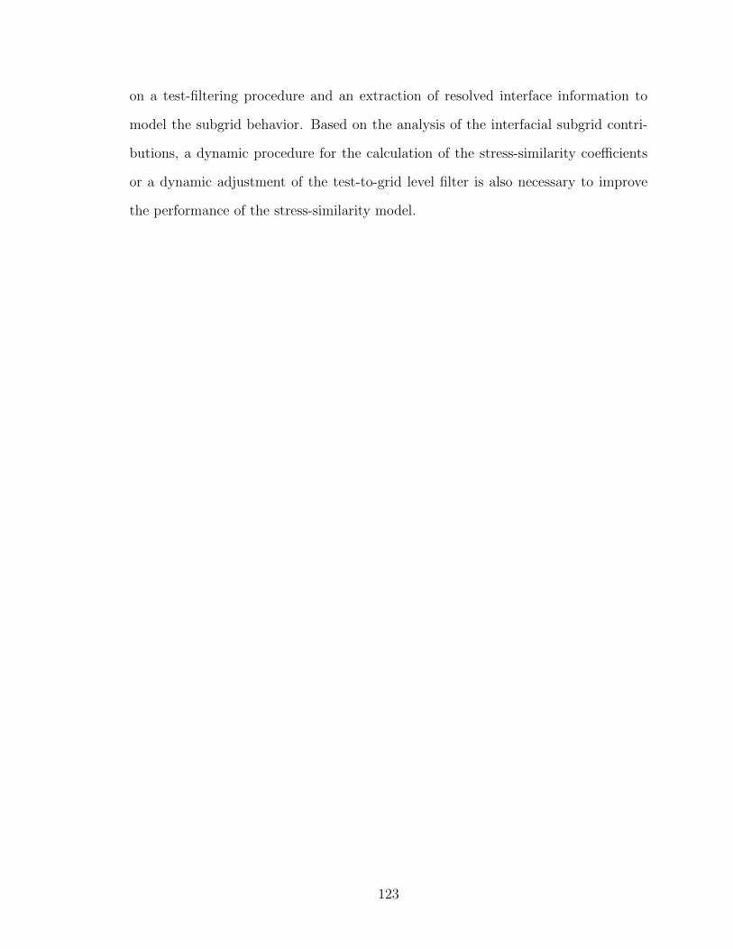
on a test-filtering procedure and an extraction of resolved interface information to
model the subgrid behavior. Based on the analysis of the interfacial subgrid contri-
butions, a dynamic procedure for the calculation of the stress-similarity coefficients
or a dynamic adjustment of the test-to-grid level filter is also necessary to improve
the performance of the stress-similarity model.
123
CHAPTER 5
Summary and Conclusions
5.1 Summary
The interaction of turbulence with a deformable interface separating two phases has
been studied with highly-resolved numerical simulations of multiphase flows relevant
to the marine industry. Two canonical flows including the phase inversion problem
and the plunging-breaking wave problem are studied with the direct numerical sim-
ulations approach to resolve the most active turbulent scales in both phases and to
accurately represent the evolution of the interface. The DNS data allows for an in-
depth study of the smallest scales that are not resolved using lower-fidelity numerical
tools such as large-eddy simulations. The inversion of an oil inclusion inside of a
closed domain filled with water is studied first to examine the turbulent-interfacial
scales using a simple two-dimensional domain and to compare the present findings
against previously published results. The breaking process of a three-dimensional wa-
ter wave is also simulated to determine the influence of the large density and viscosity
ratios on the turbulence-interface interaction. The a priori analysis is applied to both
canonical flows in order to determine the hierarchy of the subgrid-scale terms present
in the governing equations of multiphase large-eddy simulations. Additionally, sev-
eral approaches commonly used to model the subgrid behavior are benchmarked for
performance in multiphase applications. A structural model for the subgrid terms
124
associated with the presence of the interface is found to correlate well with the true
subgrid behavior. The model is implemented in the LES solver to study the two
canonical flows with the a posteriori approach. Finally, a complex flow involving
breaking and spilling-wave impacts on an offshore structure is examined with the
large-eddy simulations solver.
The phase-inversion problem is studied because it contains many of the relevant
features of turbulent-interfacial flows also found in the marine environment. The
unstable initial conditions of the oil result in a complex deformation of the interface
and turbulence generation due to the interaction of the two phases and also due to
the presence of no-slip boundaries. The relative importance of the the smallest inter-
facial and turbulent scales that are typically not resolved in large-eddy simulations
is examined by comparing the subgrid quantities to the resolved counterparts. The
traditional convective subgrid stress also present in single-phase LES equations is
found to be the largest subgrid contribution in the phase-inversion problem, but the
influence of the diffusive and the interfacial subgrid terms increases rapidly when the
filter size is increased. The structural modeling approach in the form of the stress-
similarity model is found to be highly correlated with the true subgrid terms during
the most energetic stages of the flow development.
The simulation of the plunging-breaking wave focuses on three-dimensional turbulent-
interfacial flow features that form upon impact of the overturning jet onto the front
face of the wave. Air cavities are entrained and filament-like structures are ejected
during impact, eventually leading to the formation of small air bubbles and water
droplets in the proximity of the free surface. The presence of the small-interfacial
features in highly-energetic regions of the flow field and the large density ratio result
in the subgrid interfacial contribution to be comparable in magnitude to the resolved
term. The convective subgrid term is also found to be important and a significant
contributor to the LES governing equations. The modeled subgrid behavior obtained
125

using the stress-similarity model is found to be less correlated with the true subgrid
terms than in the phase-inversion problem. The degraded performance of the model
is associated with non-homogeneity of the subgrid structures, the ratio of the test and
grid-level filters, and the constant-coefficient implementation of the model, resulting
in a poor localization of some regions responsible for the largest subgrid contributions.
Large-eddy simulations of the two canonical flows have been executed to study the
influence of the modeled subgrid terms in practice. The evolution of the kinetic energy
and its dissipation rate is computed using several different combinations of subgrid
term modeling. The dynamic mixed model that incorporates a similarity component
and a dissipative eddy-viscosity component is found to be the most robust model
for the convective subgrid-scale stress. The interfacial subgrid-scale model based
on the stress-similarity concept is shown to have a potential benefit to large-eddy
simulations of turbulent-interfacial flows. An appropriate resolution of the interface
is necessary because the model relies on a test-filtering procedure and an extraction
of resolved interface information to model the subgrid behavior. Additionally, based
on the analysis of the interfacial subgrid contributions, a dynamic procedure for the
calculation of the stress-similarity coefficients or a dynamic adjustment of the test-
to-gird level filter is also necessary in practical applications.
Breaking-wave impacts on a bottom-mounted vertical circular cylinder have been
simulated with large-eddy simulations. The technique used to generate and propa-
gate the regular linear and fifth-order Stokes waves is validated against experimental
results. Steep waves are propagated over a sloping seabed resulting in a series of
different types of wave impacts on the offshore structure including a regular non-
breaking steep wave, a plunging-breaking wave, and spilling-breaking waves. The
in-line force on the structure due to a wave that breaks directly in front of the cylin-
der in a plunging manner is found to be approximately 100% greater than the force
due to a steep non-breaking wave. A spilling breaker results in the in-line force
126
that is 50% greater than the non-breaking wave. The use of subgrid-scale modeling
does not influence the force and free-surface elevation prediction when non-breaking
waves are studied because of the low level of turbulence and free-surface deforma-
tion associated with non-breaking wave impacts. The significant deformation of the
free surface and near-interface turbulence generated during wave breaking result in
a large subgrid contribution that must be modeled to obtain correct in-line force
predictions. An appropriate model for the convective subgrid-scale stress must incor-
porate resolved-flow information through the scale-similarity concept because purely
dissipative eddy-viscosity type of modeling is known to behave poorly near the fluid
interface. The contribution of the interfacial subgrid model is found to be important
in replicating the peak negative in-line force on the cylinder, but a dynamic coefficient
calculation is necessary to adapt the model to the local-resolved-flow conditions.
5.2 Contributions
The major contributions of this work are highlighted here, along with a descrip-
tion of how each contribution impacts the field of numerical simulation of turbulent-
interfacial flows.
The hierarchy the subgrid-scale terms present in the governing equations of mul-
tiphase large-eddy simulations has been established for two canonical turbulent-
interfacial flows. The relative magnitudes of the subgrid terms related to turbu-
lence and the presence of the interface are quantified during the most important
stages of the flow evolution. The comparison of the maximum subgrid contri-
butions to the resolved contributions indicates that the interfacial subgrid term
can be significant in marine flows characterized by large density and viscosity
ratios. The subgrid interface information is shown to be a strong function of
the filter size and its magnitude to be of similar importance as the traditional
127

convective term also found in single-phase large-eddy simulations.
The performance of subgrid-scale models in application to multiphase flows is
evaluated through the comparison of the correlation between the modeled and
the true subgrid-scale stresses. The output of the scale-similarity structural
model is found to be highly correlated with the true subgrid-scale stress com-
puted from the direct numerical simulation data. Pure eddy-viscosity modeling
of the convective subgrid term is determined to be inappropriate for LES of
turbulent-interfacial flows.
The stress-similarity model is implemented in the LES solver to evaluate the
impact of the additional subgrid terms that are a result of the spatial filtering
across the interface separating the two immiscible phases. The model is found
to be highly sensitive to the resolution of the interfacial scales and the ratio
of the test-level to the grid-level filter. Unlike in many single-phase flows, the
stress-similarity model coefficient set equal to one is not appropriate for the
simulation of complex multiphase flows such as those involving breaking-water
waves.
Impact loads on a vertical circular cylinder due to steep-regular non-breaking
and breaking waves are predicted using large-eddy simulations. Subgrid mod-
eling of the convective term is found to be important for a correct prediction of
the maximum in-line force and the free-surface elevation occurring at the time
of wave breaking. Modeling of the subgrid interfacial term using the resolved
features of the interface may be beneficial in simulations of similar turbulent-
interfacial flows when combined with a method for a dynamic adjustment of the
model coefficient.
128
5.3 Future Work
The current implementation of the stress-similarity model in the LES solver uses a
constant user-specified coefficient. A dynamic calculation of this coefficient based on a
second level of test filtering should improve the performance of the model. However, a
method for determining a sufficient level of the interface resolution would be necessary
in order for the additional test-filtering procedure to use well-resolved information and
for the method to yield an appropriate coefficient as a function of space and time.
The evaluation of the subgrid terms for the breaking-wave flow uses a viscosity
ratio that is approximately twice the physical ratio. The hierarchy of the subgrid
terms is not anticipated to be affected by this deviation from the physical value, but
the relative magnitudes of the interfacial and the diffusive terms are likely affected.
A parametric study of the influence of the viscosity and density ratios would give a
clear guideline as to how sensitive the subgrid terms are to the phase properties.
A detailed comparison of the in-line forces on the cylinder due to impinging-
breaking waves against experimental data could clarify the benefits of the various
subgrid-scale modeling. Additionally, simulations with a fully-resolved boundary layer
on the surface of the cylinder would provide a better insight into the interaction of
the viscous boundary layer with the turbulence associated with the wave-breaking
process. A detailed description of the turbulent-interfacial features in the proximity
of a floating offshore structure may allow for a more accurate prediction of vortex-
induced vibrations and motions.
The importance of the local compressibility effects of the air pockets that are
entrained during the plunging event may be important to the process of turbulence
generation and dissipation. Baumgarten et al. (2002) have shown that the assumption
of incompressibility may result in an over-estimation of the bubble breakup energy
which may in turn affect the turbulent kinetic energy cascade. In multiphase flows
with large viscosity and density rations such as in the case of water-wave flows, the
129

compressibility effects are likely to be a strong function of the severity of the plunging
event and thus their relative impact on the evolution of the flow should be considered
in the next stage of this work.
130
BIBLIOGRAPHY
Apelt, C. J. and Piorewicz, J. Laboratory studies of breaking wave forces acting onvertical cylinders in shallow water. Coastal Engineering, 11:263–282, 1987.
Bardina, J., Ferziger, J. H., and Reynolds, W. C. Improved subgrid models for largeeddy simulation. Journal of AAIA, 80:1357, 1980.
Baumgarten, C., Stegemann, J., and Merker, G. A new model for cavitation inducedprimary break-up of diesel sprays. Zaragoza, 9:11, 2002.
Brackbill, J. U., Kothe, D. B., and Zemach, C. A continuum method for modelingsurface tension. Journal of Computational Physics, 100:335–354, 1992.
Bredmose, H., Slabiak, P., Sahlberg-Nielsen, L., and Schlutter, F. Dynamic excita-tion of monopiles by steep and breaking waves. experimental and numerical study.In ASME2013 32nd International Conference on Ocean, Offshore and Arctic En-gineering, 2013.
Carati, D., Ghosal, S., and Moin, P. On the representation of backscatter in dynamiclocalization models. Physics of Fluids, 7:606–616, 1995.
Chakrabarti, S. K., Kriebel, D., and Berek, E. P. Forces on a single pile caisson inbreaking waves and current. Applied Ocean Research, 19:113–140, 1997.
Chan, E. S. and Melville, W. Plunging wave forces on surface-piercing structures. InJournal of Offshore Mechanics and Arctic Engineering, 1989.
Chan, E.-S., Cheong, H.-F., and Tan, B.-C. Laboratory study of plunging waveimpacts on vertical cylinders. Coastal Engineering, 25:87–107, 1995.
Chesnel, J., Menard, T., Reveillon, J., and Demoulin, F.-X. Subgrid analysis of liquidjet atomization. Atomization and Sprays, 21:41–67, 2011a.
Chesnel, J., Reveillon, J., Menard, T., and Demoulin, F. X. Large eddy simulationof liquid jet atomization. Atomization and Sprays, 21:711–736, 2011b.
Chong, M. S., Perry, A. E., and Cantwell, J. A general classification of threedimen-sional flow fields. Physics of Fluids, 2:765–777, 1990.
Christensen, E. D., Bredmose, H., and Hansen, E. A. Extreme wave forces and waverun-up on offshore wind turbine foundations. In Copenhagen Offshore Wind, 2005.
131

Christensen, E. D. and Deigaard, R. Large eddy simulation of breaking waves. CoastalEngineering, 42:53–86, 2001.
Chumakov, S. G. Subgrid models for large eddy simulation: scalar flux, scalar dis-sipation and energy dissipation. PhD thesis, University of Wisconsin - Madison,2005.
Cook, A. W. Determination of the constant coefficient in scale similarity models ofturbulence. Physics of Fluids, 9:1485–1487, 1997.
Damian, S. M. Description and utilization of interfoam multiphase solver. Technicalreport, International Center for Computational Methods in Engineering, 2012.
de Ridder, E. J., Aalberts, P., van den Berg, J., Buchner, B., and Peeringa, J. Thedynamic response of an offshore wind turbine with realistic flexibility to breakingwave impact. In ASME 2011 30th International Conference on Ocean, Offshoreand Arctic Engineering, 2011.
de Villiers, E. The potential of large eddy simulation for the modeling of wall boundedflows. PhD thesis, Imperial College of Science, Technology and Medicine, 2006.
Dean, R. G. and Dalrymple, R. A. Water wave mechanics for engineers and scientists.World Scientific, 1991.
Ferziger, J. H. and Peric, M. Computational methods for fluid dynamics. SpringerBerlin, 1996.
Frigaard, P., Anderson, T. L., Ramirez, J. R. R., Sorensen, S. P. H., Martinelli, L.,Lamberti, A., Troch, P., de Vos, L., Kisacik, D., Stratigaki, V., Zou, Q., Monk, K.,Vandamme, J., Damsgaard, M. L., and Gravesen, H. Loads on entrance platformsfor offshore wind turbines. In HYDRALAB III Joint User Meeting Hannover, 2010.
Fureby, C. Iles and les of complex engineering turbulent flows. Journal of FluidsEngineering, 129:1514–1523, 2007.
Germano, M. A proposal for a redefinition of the turbulent stresses in the filterednavierstokes equations. Physics of Fluids, 29:2323–2324, 1986.
Germano, M., Pimoelli, U., Moin, P., and Cabot, W. H. A dynamic subgrid-scaleeddy viscosity model. Physics of Fluids, 3:1760–1765, 1991.
Goda, Y., Haranaka, S., and Kitahata, M. Study of impuslive breaking wave forceson piles. Technical report, Port and Harbour Research Institute, 1966.
Gullbrand, J. and Chow, F. K. The eect of numerical errors and turbulence modelsin large-eddy simulations of channel ow, with and without explicit ltering. Journalof Fluid Mechanics, 495:323–341, 2003.
Hildebrandt, A. and Schlurmann, T. Breaking wave kinematics, local pressures, andforces on a tripod structure. In Coastal Engineering, 2012.
132

Iafrati, A. Numerical study of the effects of the breaking intensity on wave breakingflows. Journal of Fluid Mechanics, 622:371–411, 2009.
Iafrati, A. Energy dissipation mechanisms in wave breaking processes: Spilling andhighly aerated plunging breaking events. Journal of Geophysical Research, 116:1–22, 2011.
Iafrati, A., Onorato, M., and Babanin, A. Analysis of wave breaking events generatedas a result of a modulation instability. In 29th Symposium on Naval Hydrodynamics,2012.
Irschik, K., Sparboom, U., and Oumeraci, H. Breaking wave characteristics for theloading of a slender pile. In 28th Int. Conf. Coastal Eng., ICCE, 2002.
Issa, R. I. Solution of the implicitly discretized fluid flow equations by operator-splitting. Journal of Computational Physics, 62:40–65, 1986.
Jacobsen, N. G., Fuhrman, D. R., and Fredsoe, J. A wave generation toolbox for theopen-source cfd library: Openfoam®. International Journal of Numerical Methodsin Fluids, 2011.
Jasak, H. Error Analysis and Estimation for Finite Volume Method with Applicationsto Fluid Flow. PhD thesis, Imperial College, University of London, 1996.
Jasak, H. High resolution NVD differencing scheme for arbitrarily unstructuredmeshes. International Journal for Numerical Methods in Fluids, 31:431–449, 1999.
Kim, J., Moin, P., and Moser, R. Turbulence statistics in fully developed channelflow at low reynolds number. Journal of Fluid Mechanics, 177:133–166, 1987.
Kim, W. and Menon, S. A new dynamic one-equation subgrid-scale model for largeeddy simulation. In 33rd Aerospace Sciences Meeting and Exhibit, 1995.
Kornev, N. V., Tkatchenko, I. V., and Hassel, E. A simple clipping procedure for thedynamic mixed model based on taylor series approximation. Communications inNumerical Methods in Engineering, 22:55–61, 2006.
Labourasse, E., Lacanette, D., Toutant, A., Lubin, P., Vincent, S., Lebaigue, O.,Caltagirone, J.-P., and Sagaut, P. Towards large eddy simulation of isothermaltwo-phase flows; governing equations and a priori tests. International Journal ofMultiphase Flow, 33:1–39, 2007.
Lakehal, D. and Liovic, P. Turbulence structure and interaction with steep breakingwaves. Journal of Fluid Mechanics, 674:522–577, 2011.
Larocque, J., Vincent, S., Lacanette, D., Lubin, P., and Caltagirone, J.-P. Parameterstudy of LES subgrid terms in a turbulent phase separation flow. InternationalJournal of Heat and Fluid Flow, 31:536–544, 2010.
133
Lilly, D. K. A proposed modification of the germano subgrid-scale closure method.Physics of Fluids, 4:633–635, 1992.
Liu, S., Meneveau, C., and Katz, J. On the properties of similarity subgrid-scale mod-els as deduced from measurements in a turbulent jet. Journal of Fluid Mechanics,275:83–119, 1994.
Lubin, P. Large Eddy Simulation of plunging breaking waves. PhD thesis, UniversiteBordeaux, 2004.
Lubin, P., Glockner, S., Kimmoun, O., and Branger, H. Numerical study of thehydrodynamics of regular waves breaking over a sloping beach. European Journalof Mechanics B/Fluids, 30:552–564, 2011.
Lubin, P., Vincent, S., Abadie, S., and Caltagirone, J.-P. Three-dimensional largeeddy simulation of air entrainment under plunging breaking waves. Coastal Engi-neering, 53:631–655, 2006.
Meneveau, C. and Katz, J. Scale-invariance and turbulence models for large-eddysimulation. Annual Review Fluid Mechanics, 32:1–32, 2000.
Meneveau, C., Lund, T. S., and Cabot, W. H. A lagrangian dynamic subgrid-scalemodel of turbulence. Journal of Fluid Mechanics, 319:353–385, 1996.
Moin, P. and Mahesh, K. Direct numerical simulation: A tool in turbulence research.Annual Review Fluid Mechanics, 30:539–578, 1998.
Morison, J. The force exerted by surface waves on piles. Petroleum Transactions,AIME, 1950.
Nielsen, A. W., Schlutter, F., Sorensen, J. V. T., and Bredmose, H. Wave loads ona monopile in 3D waves. In ASME 2012 31st International Conference on Ocean,Offshore and Arctic Engineering, 2012.
Olsson, E., Kreiss, G., and Zahedi, S. A conservative level set method for two phaseflow ii. Journal of Computational Physics, 225:785–807, 2007.
Olsson, E. and Kreiss, G. A conservative level set method for two phase flow. Journalof Computational Physics, 210:225–246, 2005.
Park, N., Yoo, J. Y., and Choi, H. Toward improved consistency of a priori tests witha posteriori tests in large eddy simulation. Physics of Fluids, 17, 2005.
Perlin, M., Choi, W., and Tian, Z. Breaking waves in deep and intermediate waters.Annual Review Fluid Mechanics, 45:115–145, 2013.
Piro, D. J. A Hydroelastic Method for the Analysis of Global Ship Response Due toSlamming Events. PhD thesis, University of Michigan, 2013.
Pope, S. B. Turbulent Flows. Cambridge University Press, 2000.
134
Ramirez, J., Frigaard, P., Andersen, T. L., and Christensen, E. D. Breaking wave ona slender cylinder: comparison of experimental data and numerical results. In 31stInternational Conference on Ocean, Offshore and Arctic Engineering, 2012.
Rusche, H. Computational Fluid Dynamics of Dispersed Two-Phase FLows at HighPhase Fractions. PhD thesis, Imperial College of Science, Technology & Medicine- University of London, 2002.
Sagaut, P. Large eddy simulation for incompressible flows. Springer Berlin, 2001.
Salvetti, M. V. and Banerjee, S. A priori tests of a new dynamic subgrid scale modelfor finite difference large eddy simulations. Physics of Fluids, 7:2831–2847, 1995.
Sarghini, F., Pimoelli, U., and Balaras, E. Scale-similar models for large-eddy simu-lations. Physics of Fluids, 11:1596–1607, 1999.
Scardovelli, R. and Zaleski, S. Direct numerical simulation of free-surface and inter-facial flow. Annual Review of Fluid Mechanics, 31:567–603, 1999.
Shen, L. and Yue, D. K. P. Large-eddy simulation of free-surface turbulence. Journalof Fluid Mechanics, 440:75–116, 2001.
Smagorinsky, J. General circulation experiments with the primitive equations. Tech-nical report, Department of Commerce - Weather Bureau, 1963.
Song, C. and Sirviente, A. I. A numerical study of breaking waves. Physics of Fluids,16:2649–2667, 2004.
Toutant, A., Chandesris, M., Jamet, D., and Lebaigue, O. Jump conditions forfiltered quantities at an under-resolved discontinuous interface. part 1: Theoreticaldevelopment. International Journal of Multiphase Flow, 35:1100–1118, 2009.
van Haren, S. W. Testing DNS capability of OpenFOAM and STAR-CCM+. Master’sthesis, Delft University of Technology, 2011.
Vincent, S., Larocque, J., Lacanette, D., Toutant, A., Lubin, P., and Saguat, P.Numerical simulation of phase separation and a priori two-phase LES filtering.Computers and Fluids, 37:898–906, 2008.
Vreman, B., Geurts, B., and Kuerten, H. A priori tests of large eddy simulation of thecompressible plane mixing layer. Journal of Engineering Mathematics, 29:299–327,1995.
Watanabe, Y., Saeki, H., and Hosking, R. J. Three-dimensional vortex structuresunder breaking waves. Journal of Fluid Mechanics, 545:291–328, 2005.
Whitham, G. B. Linear and Nonlinear Waves. John Wiley & Sons, 1974.
Wienke, J., Sparboom, U., and Oumeraci, H. Breaking wave impact on a slendercylinder. In Coastal Engineering Conference, 2001.
135
Zang, J., Taylor, P. H., and Tello, M. Steep wave and breaking wave impact on offshorewind turbine foundations - ringing re-visited. In 25th International Workship onWater Waves and Floating Bodies, 2010.
Zang, Y., Street, R. L., and Koseff, J. R. A dynamic mixed subgrid-scale model andits application to turbulent recirculating flows. Physics of Fluids, 5:3186, 1993.
Zhao, Q., Armfield, S., and Tanimoto, K. Numerical simulation of breaking waves bya multi-scale turbulence model. Coastal Engineering, 51:53–80, 2004.
136