Embed Size (px)
Citation preview

NUMERICAL ANALYSIS OF BIOLOGICAL AND
ENVIRONMENTAL DATA
Lecture 11.Hypothesis Testing

Randomisation testsSimple introductory example
Monte Carlo permutation tests
HYPOTHESIS TESTINGHYPOTHESIS TESTING
Spatial biogeographical data
Mantel tests
Partial Mantel test
Spatial and temporal data
Importance of permutation tests
Types of permutation tests
Palaeoecological stratigraphical data
Time-duration tests
Impacts of volcanic ash of terrestrial and aquatic systems
Impacts of land-use on lake-water activity
Impacts of Picea Abies (spruce) on lake-water acidity
Ecological data
RDA as a tool for reduced-rank regression
Impact of seasonal sheep grazing on grasslands
Weeds in Sweden
Short-term vegetational change in fen meadow
Field eco-toxicology experiments
Other numerical tools

RANDOMISATION TESTS
SIMPLE INTRODUCTORY
EXAMPLEMandible lengths of male and female jackals in Natural History
Museum Male 120 107 110 116 114 111 113 117 114 112 mm
Female 110 111 107 108 110 105 107 106 111 111 mm
Is there any evidence of difference in mean lengths for two sexes? Male mean larger than female mean.
Null hypothesis (Ho) – no difference in mean lengths for two
sexes, any difference is purely due to chance. If Ho consistent
with data, no reason to reject this in favour of alternative hypothesis that males have a larger mean that females.
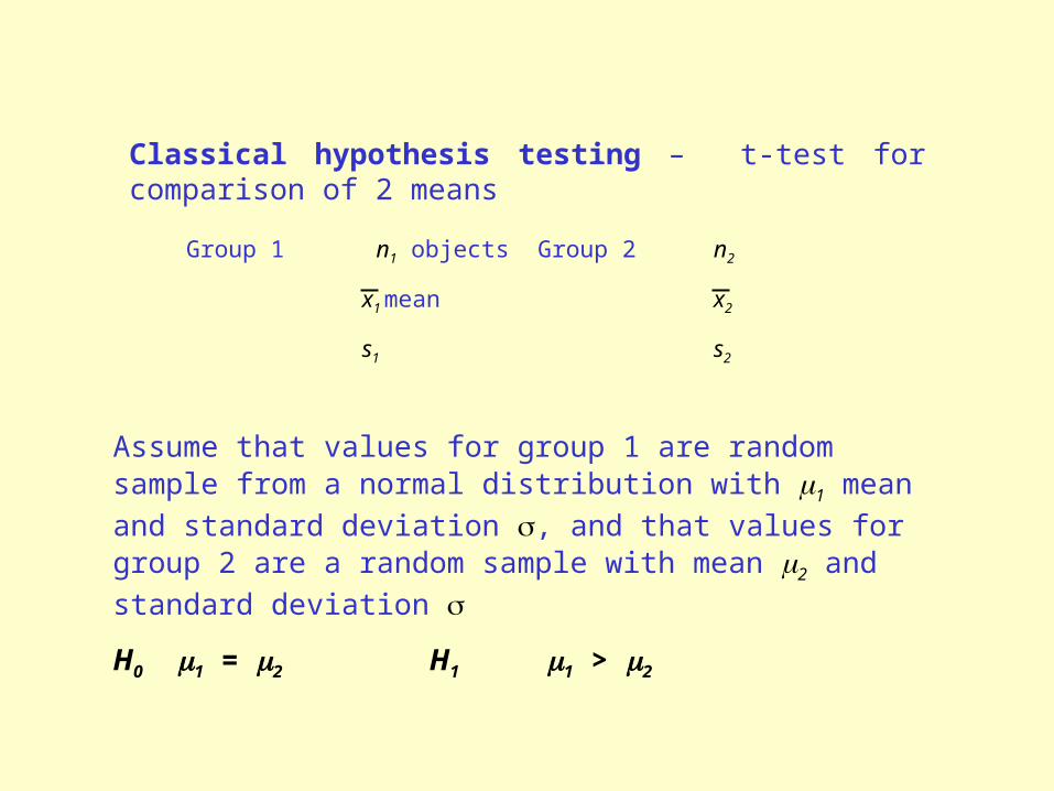
Classical hypothesis testing – t-test for comparison of 2 means
Group 1 n1 objects Group 2 n2
x1 mean x2
s1 s2
Assume that values for group 1 are random sample from a normal distribution with 1 mean and standard deviation , and that values for group 2 are a random sample with mean 2 and standard deviation
H0 1 = 2 H1 1 > 2
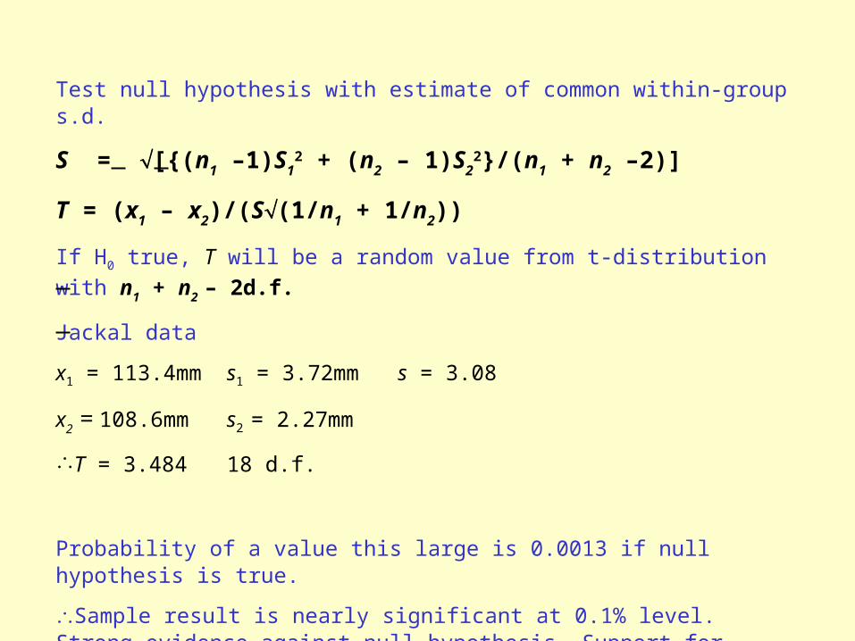
Test null hypothesis with estimate of common within-group s.d.
S = [{(n1 –1)S12 + (n2 – 1)S2
2}/(n1 + n2 –2)]
T = (x1 – x2)/(S(1/n1 + 1/n2))
If H0 true, T will be a random value from t-distribution with n1 + n2 –
2d.f.
Jackal data
x1 = 113.4mm s1 = 3.72mm s = 3.08
x2 = 108.6mm s2 = 2.27mm
T = 3.484 18 d.f.
Probability of a value this large is 0.0013 if null hypothesis is true.
Sample result is nearly significant at 0.1% level. Strong evidence against null hypothesis. Support for alternative hypothesis.

ASSUMPTIONS OF T-TEST
1. Random sampling of individuals from the populations of interest
2. Equal population standard deviations for males
and females
3. Normal distributions within groups

ALTERNATIVE APPROACHIf there is no difference between the two sexes, then the length distribution in the two groups will just be a typical result of allocating 20 lengths at random into 2 groups each of size 10. Compare observed difference with distribution of differences found with random allocation.
TEST:
1. Find mean scores for male and female and difference D0 for observed data.
2. Randomly allocate 10 lengths to male group, remaining 10 to female. Calculate D1.
3. Repeat many times (n e.g. 999 times) to find an empirical distribution of D that occurs by random allocation. RANDOMISATION DISTRIBUTION.
4. If D0 looks like a ’typical’ value from this randomisation distribution, conclude that allocation of lengths to males and females is essentially random and thus there is no difference in length values. If D0 unusually large, say in top 5% tail of randomisation distribution, observed data unlikely to have arisen if null hypothesis is true. Conclude alternative model is more plausible.
If D0 in top 1% tail, significant at 1% level
If D0 in top 0.1% tail, significant at 0.1% level

The distribution of the differences observed between the mean for males and the mean for females when 20 measurements of mandible lengths are randomly allocated, 10 to each sex. 4999 randomisations.

x1 = 113.4mm x2 = 108.6mm D0 = 4.8mm
Only nine were 4.8 or more, including D0.
Six were 4.8 2 > 4.8
9Significance level = 5000 = 0.0018 = 0.18%
(cf. t-test 0.0013 0.13%)
20C10 = 184,756. 5000 only 2.7% of all possibilities.

THREE MAIN ADVANTAGES
1. Valid even without random samples.
2. Easy to take account of particular features of data.
3. Can use 'non-standard' test statistics.
Tell us if a certain pattern could or could not be caused/arisen by chance. Completely specific to data set.
RANDOMISATION TESTS AND MONTE CARLO PERMUTATION TESTS
If all data arrangements are equally likely, RANDOMISATION TEST with random sampling of randomisation distribution. Otherwise, MONTE CARLO PERMUTATION TEST.
Validity depends on validity of permutation types for particular data-type – time-series stratigraphical data, spatial grids, repeated measurements (BACI). All require particular types of permutations.

USEFUL REVIEWSPALAEOECOLOGY
Birks (1993) INQUA Newsletter on Data-Handling Methods 14, 2-8.
ECOLOGY
Crowley (1992) Ann. Review Ecology & Systematics 23, 405-447.
Strong (1980) Synthese 43, 271–285
Harvey et al. (1983) Ann. Rev. Ecol. System. 14, 189–211
Manly, B.F.J. (1997)
Randomization, bootstrap and Monte Carlo methods in biology
Good, P. (2000)
Permutation tests – A practical guide to resampling methods for testing hypotheses
Good, P. (2005)
Introduction to statistics through resampling methods and R/S-PLUS
Gotelli, N.J. & Graves, G.R.
(1996)
Null models in ecology
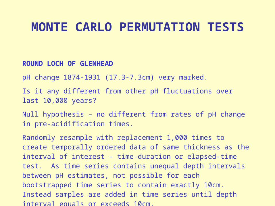
ROUND LOCH OF GLENHEAD
pH change 1874-1931 (17.3-7.3cm) very marked.
Is it any different from other pH fluctuations over last 10,000 years?
Null hypothesis – no different from rates of pH change in pre-acidification times.
Randomly resample with replacement 1,000 times to create temporally ordered data of same thickness as the interval of interest – time-duration or elapsed-time test. As time series contains unequal depth intervals between pH estimates, not possible for each bootstrapped time series to contain exactly 10cm. Instead samples are added in time series until depth interval equals or exceeds 10cm.
MONTE CARLO PERMUTATION TESTS


Rate (pH change per cm)

Response variable(s) Y e.g. lake-water pH, sediment LOI, tree pollen stratigraphy
Predictor variable(s) X e.g. charcoal, age, land-use indicators, climate
Also covariables
Basic statistical model:Y = BX
Y X Method
1 1 Simple linear regression
1 >1 Multiple linear regression, principal components regression, partial least squares (PLS)
>1 ≥1 Redundancy analysis (= constrained PCA, reduced-rank regression, PCA of y with respect to x, etc.)
Statistical testing by Monte Carlo permutation tests to derive empirical statistical distributions
Variance partitioning or decomposition to evaluate different hypotheses.
STATISTICAL METHODS FOR TESTING COMPETING CAUSAL
HYPOTHESES

BASIS OF MONTE CARLO PERMUTATION TESTS IN CANOCO
Null hypothesis – species are unrelated to environmental data
Alternative hypothesis – species are related to environmental data
STATISTICAL TEST
1. Select an appropriate test statistic to express how strongly species data respond to environment (e.g. r, t-ratio, F ratio).
2. Calculate test statistic for data S0.
3. Determine a reference distribution for the test statistic under the null hypothesis. Reference distribution shows the values to be expected under the null hypothesis that species are unrelated to environment.
4. Calculate the significance level, i.e. the probability that S0 or larger values occur in the reference distribution.
Crux of all standard tests is that the reference distribution can be derived mathematically from the assumptions of the test, e.g. F-ratio in regression or ANOVA and F-distribution and hence tables of F-distribution.

MONTE CARLO PERMUTATION TEST
Reference distribution is determined from the data themselves, without the assumptions of normality and without mathematical derivations. Its basis lies in the observation that under the null hypothesis the samples in the species data can be randomly linked with the samples in the environmental data.
Under the null hypothesis, each permutation of the samples is equally likely. Each permutation leads to a new data set from which the test statistic can be calculated. The reference distribution is therefore the distribution of the test statistic in the permuted data sets.
STEPS
1. Choose test statistic that expresses how strongly the species data respond to the environment. In CANOCO there are two test statistics that both have the form of an F-ratio.
2. Calculate the test statistic for the data, F0.
3. Generate K new data sets that are equally likely under the null hypothesis. In CANOCO this is done by randomly permuting the samples in the species data (response data) while keeping the environmental (and covariable data) data fixed.

4. Calculate the test statistic for each new data set
5. Calculate the Monte Carlo significance level
KFFFF 321
1
0
KFFKof Number
Cannot generate all possible permutations, so should do a reasonable number. If K = 10,000, little random variation but not strictly necessary. Also takes computer time. For 5% significance level, good compromise is at least 199 permutations for the test.

TYPES OF PERMUTATION TESTS AVAILABLE IN CANOCO 3 & 4
Validity of permutation test depends on the type of permutation for particular research design
1. Completely randomised designed experiments, completely random permutation appropriate. Unrestricted permutation yields completely random permutations.
2. If data are from time series, line transect, or rectangular spatial grid, restricted permutation. For ‘linear’ data, bend series into circle so that start and end meet. Randomly match X and Y. For grid, wrap data around a torus.
3. Randomised block design, permutation must be conditioned on blocks. e.g. farm types as covariables, permutation within blocks guarantees permutations are within farms.
4. Repeated measurement design, each unit must have been recorded the same number of times. Data for consecutive samples in time must be given consecutive numbers in the input files. Use covariables to define blocks.
5. BACI – before-after-control-impact studiesabundance = plot effect + time + lime effect + error
covariablecovariabless

Fig. 1. Ecological implications of the different randomization procedures for the correlation between two spatially auto-correlated variables. Here each variable sampled over a two-dimensional area is represented by a layer. a) Randomization that implies no spatial structure among variables or species; b) Restricted randomization within region, which implies some degree of spatial structure at the regional scale but no spatial structure within regions; c) Restricted randomization keeping the sequence of the data fixed by doing a toroidal shift (i.e. the spatial pattern at the variable or species is preserved); and d) Restricted randomization based on the degree of spatial autocorrelation of the observed data.

ADDITIONAL PERMUTATION TESTS AVAILABLE IN CANOCO 4
Split-Plot Design
Hierarchical design with two levels of units - WHOLE PLOTS containing SPLIT PLOTS e.g. samples within different mountains, plots within stands, plots along transects, quadrats within time series (permanent plots).
Can permute WHOLE PLOTS or SPLIT PLOTS or both.
Whole Plots should be of equal size.
Effect of environmental variables that vary within WHOLE PLOTS can be tested by permuting split plots completely at random within whole plots without permuting whole plots. Whole Plots restrict the permutations in the same way as blocks but without the need to define block-defining covariables.
Within WHOLE PLOT or SPLIT PLOT, can then have time series or line transect, spatial grids, or freely exchangeable.

WHAT IS SHUFFLED IN CANOCO PERMUTATION TESTS?
1. No covariables in the analysis (or covariables are used to define blocks) it does not matter if the samples in the species data or the environmental data are permuted. Wide choice of possible test statistics.
Null hypothesis of the test is the OVERALL NULL MODEL - species are unrelated to the environmental data (within blocks, if defined). Simple hypothesis test, comparable to overall F-test is regression analysis.
2. If covariables are present, e.g. does one variable have an effect on the species after taking into account the effect of another variable.
e.g. does nutrient pollution affect species composition after taking into account the natural variation in salinity of the water?
In regression analysis, such questions are addressed by a t-test or, if the effect of more than one variable is of interest, a partial F-test. PARTIAL or CONDITIONAL tests.
Need a multivariate form of such a test that does not assume multivariate normality.

Effect of environmental variables X on the species data Y in the presence of the
covariables Z.
Test the null hypothesis that all elements of C = 0 when elements of B are
unknown.
To test H0 C = 0 (i.e. the effect of X), proposed solutions:
1. Permute the rows of the species data Y
2. Permute the rows of the environmental data X (CANOCO 2)
3. Permute the residuals Er of the regression of Y on Z REDUCED MODEL or NULL MODEL
(CANOCO 3,4)
4. Permute the residuals of Ef of the regression of Y on Z and XFULL MODEL (CANOCO 3,4)
Y = ZB + XC + E
covariablesrandom errors
regression coefficients
environmental variables
species data
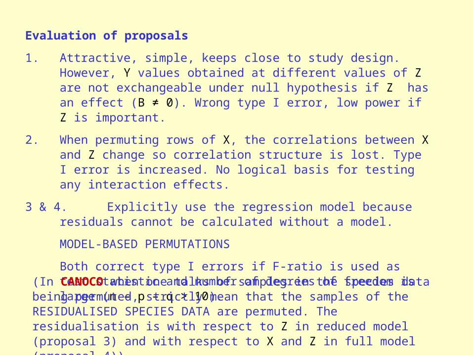
Evaluation of proposals
1. Attractive, simple, keeps close to study design. However, Y values obtained at different values of Z are not exchangeable under null hypothesis if Z has an effect (B ≠ 0). Wrong type I error, low power if Z is important.
2. When permuting rows of X, the correlations between X and Z change so correlation structure is lost. Type I error is increased. No logical basis for testing any interaction effects.
3 & 4. Explicitly use the regression model because residuals cannot be calculated without a model.
MODEL-BASED PERMUTATIONS
Both correct type I errors if F-ratio is used as test statistic and number of degrees of freedom is large (n – p – q > 10).
(In CANOCO when one talks of samples in the species data being permuted, strictly mean that the samples of the RESIDUALISED SPECIES DATA are permuted. The residualisation is with respect to Z in reduced model (proposal 3) and with respect to X and Z in full model (proposal 4)).

Model-based permutation
Permutation test of the effect of X, adjusted for the possible effect of Z.
1. Choose test statistic F ratio of partial F-test to test the null hypothesis C = 0
Regress species data on Y on covariable data Z, then add environmental variables X to regression, giving residual sum of squares RSSz and RSSz + x,
respectively.
Calculate F ratio for testing C = 0
sum of all canonical eigenvalues (with covariables & environmental variables)
2. Calculate test statistic for data, F0
3. Generate K new data sets that are equally likely under the null hypothesis.
Two substeps
1. Regress Y on Z, yielding fitted values Ŷ and residuals E with E = Y – Ŷ
2. Permute the rows of E to yield E* and calculate new data Y* = Ŷ + E*
n-p-qq
xz
z
RSSRSSRSS
F xz

4. Calculate the test statistic for each new data set Y*.
As in step 1 with Y* replacing Y giving F ratiosF1, F2, F3, F4 Fk
5. Calculate Monte Carlo significance level
Place F0 among F1, F2 ... Fk and determine the proportion of values greater than or equal to F0
This is the procedure for "Test of significance for all canonical axes" or "Test based on the trace statistic".
ALSO - test statistic based on first canonical eigenvalue or axis one 1
F = 1 / (RSSz+1 / (n – p – q))
residual sum of squares of model with covariables fitted and first ordination axis of environmental data (rank 1 restriction on matrix of regression coefficients C) Maximum power against alternative hypothesis (H1) that there is a single dominating gradient that determines the relation between species and environment.

TESTS OF STATISTICAL SIGNIFICANCE IN CANONICAL
ANALYSISComparison of the methods of permutation of raw data or residuals in terms of the permuted fractions of variation, in the presence or absence of a matrix of covariables W. Fractions of variation: (a) is the variation of matrix Y explained by X alone; (c) the variation explained by W alone; (b) the variation explained jointly by X and W, and (d) the residual variation.
Without covariables With matrix W of covariables
(a) (d) (a) (b) (c) (d)
Explained by X
Unexplained Explained by X Unexplained
variation Explained by W variation
environmental data
covariable

CANOCO
## Without covariables With covariables
2 2 Permute raw data
Permute [a + d] Permute [a + b + c + d]1
Permute residuals
3, 4 3 * Reduced model
Equivalent to permuting raw data
Permute [a + d]
4 4 * Full model Permute [d] Permute [d]1 Permutation of raw data may result in unstable (often inflated) type I error when the covariable contains outliers. This does not occur, however, when using restricted permutations of raw data within groups of a qualitative covariable, which gives an exact test.
Reduced or null model
Residuals of reduced model of covariables only (a + d)
Full model Residuals of a full model of explanatory variable and covariables (d)
Not enough known yet to decide whether to use reduced or full model. Needs experiments with simulated data, assessment of type I and type II errors, precision of p-values, etc.

WHAT IS PERMUTED IN CANOCO – A SUMMARY
If no covariables or conditioning variables, biological data or environmental data can be permuted.
In partial models with conditioning variables, cannot permute biological data as they are dependent on the conditional variables and cannot permute the constraining environmental data as they correlate with the conditional variables.
Residuals are exchangeable if they are independent and identically distributed.
Reduced model permutes residuals after considering the conditional variables.
Full model permutes residuals after considering the conditional variables and the constraining variables.

DISTANCE-BASED REDUNDANCY ANALYSIS
Legendre & Anderson (1999) Ecol. Monogr.
Extends RDA and associated battery of permutation tests to use any ecologically reasonable similarity or dissimilarity coefficient.
1. Calculate DC between samples
2. Transform to principal co-ordinates, including a correction for negative eigenvalues Y
3. Create a matrix of dummy variables (or environmental variables) X (and Z)
4. Do a RDA using Y and X (and Z)
5. Permutation tests for particular model.


REGRESSION AND ANALYSIS OF VARIANCE USING PERMUTATION
TESTSIdeal for data with non-normal error structure.
1. Multiple linear regression (ordinary or forced through the origin) with permutation tests (permutation of values y; permutation of residuals of the full regression model).
MLR www.fas.umontreal.co/biol/legendre
2. Non-parametric multivariate analysis of variance.
Use any symmetric distance or dissimilarity measure as measure of sample differences. Assess statistical significance by permutation tests (restricted permutation of raw data; permutation of residuals of the full model; permutation of residuals of the reduced model).
Designs - one-way design; two-way nested design; two-way crossed design.
Anderson, M.J. (2001) Austral. Ecology 26, 32-46
NPMANOVA and PERMANOVA_2factor www.stat.auckland.ac.nz/~mja

3. Generalised distance-based multivariate analysis for a linear model.
Multivariate multiple regression of any symmetric distance matrix for response variables Y(n x m). Predictor variables (X n x q) contain variables of interest for testing the multivariate null hypothesis of no relationship between Y and X on the basis of the distance matrix chosen.
X may contain the codes of an ANOVA model (design matrix) or one or more explanatory variables (e.g. environmental variables).
Can include covariables in the analysis.
Permutations - unrestricted of raw data; residuals under a reduced model; residuals under a full model.
McArdle, B.H. & Anderson, M.J. (2001) Ecology 82, 290-297
Anderson, M.J. & Robinson, J. (2001) Australian and New Zealand J. Statistics 43, 75-88
DISTLM www.stat.auckland.ac.nz/~mja
DISTLM-forward www.stat.auckland.ac.nz/~mja

WARNINGS
'Non-parametric' does not mean 'no assumptions'
1. Traditional parametric univariate ANOVA assumptions:
(i) distribution of errors is normal
(ii) data are independent
(iii) any treatment effects are additive
(iv) variances are homogenous among groups
Permutation tests allow only assumption (i) to be ignored. Permutation tests still require replicate observations to be independent and identically distributed, the errors to come from the same distribution (same common variance) and be independent of one another. Use of permutation tests does not avoid assumptions of independence or homogenous variances and as a linear ANOVA model is being used, the assumption of additivity is still important.

2. Assumptions of independence applies to observations, not variables.
3. Significant results can be caused by heterogeneous dispersions or variances.
4. Pair-wise a posteriori tests are not corrected for experiment-wise type I error rates. Thus if one uses 0.05 for tests, you can expect a significant result in 1 out of every 20 tests by chance alone.
Do obtain the exact Monte Carlo permutation value. Onus on the user is how to interpret the p-value obtained (e.g. ? Use Bonferroni correction)
5. Cannot enumerate all possible permutations. Well worth using 999 or even 4999 permutations. Good programs will tell you what the maximum number of possible permutations is for a particular test (data and design matrix).

TIME-DURATION TEST
Round Loch of Glenhead example
Is the pH change between 1874 and 1931 any different from any other pH fluctuations in the last 10,000 years?
Randomly resample with replacement 1000 times to make temporally ordered data of same duration or thickness as 1874-1931. Compare observed pH change with pH change in the 1000 bootstraps.
How many times is the rate of interest (Obs) exceeded in the 1000 bootstraps?
Exact Monte Carlo probability =
(Number of bootstraps Obs) + 1 (for Obs) Number of bootstraps + 1 (for Obs)
p = 0.021

A.F. Lotter & H.J.B. Birks (1993)
J. Quat. Sci. 8, 263 - 276
11000 BP
? Any impact on terrestrial and aquatic systems
Also:
H.J.B. Birks & A.F. Lotter
(1994) J. Paleolimnology 11, 313 - 922
A F Lotter et al. (1995) J. Paleolimnology 14, 23 - 47
ASSESSING IMPACTS OF LAACHER SEE VOLCANIC ASH ON TERRESTRIAL AND
AQUATIC ECOSYSTEMS

Map showing the location of Laacher See (red star), as well as the location of the sites investigated (blue circle). Numbers indicate the amount of Laacher See Tephra deposition in millimetres (modified from van den Bogaard, 1983).


Loss-on-ignition of cores Hirschenmoor HI-1 and Rotmeer RO-6. The line marks the transition from the Allerød (II) to the Younger Dryas (III) biozone. LST = Laacher See Tephra.

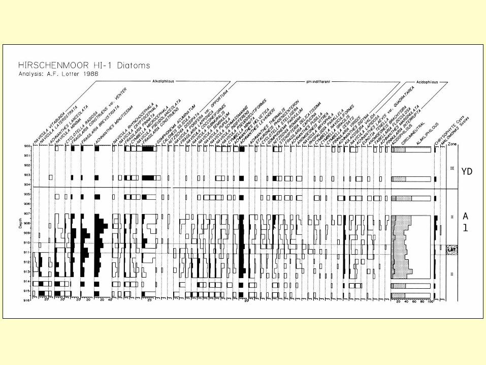
Diatoms in cores HI-1 and RO-6 grouped according to life-forms. LST = Laacher See Tephra.

Allerød
Younger Dryas

Younger Dryas
Allerød

Al
YD

Diatom-inferred pH values for cores HI-1 and RO-6. The interpolation is based on distance-weighted least-squares (tension = 0.01). The line marks the transition from the Allerød (II) to the Younger Dryas (III) biozone. LST = Laacher See Tephra.

Data
Terrestrial pollen and spores (9, 31 taxa)Aquatic pollen and spores (6, 8 taxa) RESPONSE VARIABLESDiatoms (42,54 taxa) % data
Biozone (Allerød, Allerød/Younger Dryas, Younger Dryas)
+/-
Lithology (gyttja, clay/gyttja) +/-
Depth ("age") Continuous
Ash Exponential decay process Continuous
= 0.5
x = 100
t = time
YD
211 years
Exp x-t
Time AL
EXPLANATORY VARIABLES
NUMERICAL ANALYSIS
(Partial) redundancy analysis
Restricted (stratigraphical) Monte Carlo permutation tests
Variance partitioning
Log-ratio centring because of % data
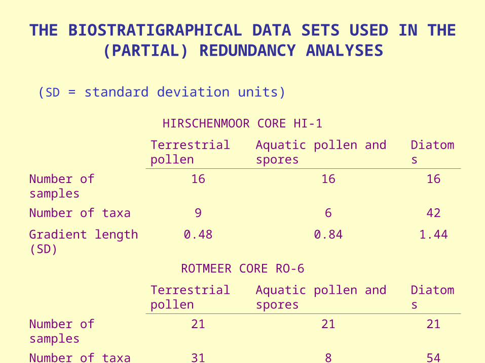
THE BIOSTRATIGRAPHICAL DATA SETS USED IN THE (PARTIAL) REDUNDANCY ANALYSES
(SD = standard deviation units)
HIRSCHENMOOR CORE HI-1
Terrestrial pollen
Aquatic pollen and spores
Diatoms
Number of samples
16 16 16
Number of taxa 9 6 42
Gradient length (SD)
0.48 0.84 1.44
ROTMEER CORE RO-6
Terrestrial pollen
Aquatic pollen and spores
Diatoms
Number of samples
21 21 21
Number of taxa 31 8 54
Gradient length (SD)
0.74 0.71 1.68

RESULTS OF (PARTIAL) RESUNDANCY ANALYSIS OF THE BIOSTRATIGRAPHICAL DATA SETS AT ROTMEER (RO-6) AND HIRSCHENMOOR (HI-1) UNDER DIFFERENT MODELS OF EXPLANATORY VARIABLES AND COVARIABLES. Entries are significance levels as assessed by restricted Monte Carlo permutation tests (n = 99)
Data Set
Site Explanatory variables Covariables Terrestria
l pollenAquatic pollen & spores
Diatoms
RO-6 Depth + biozone + ash + lithology
- 0.01a 0.01a 0.01a
HI-1 Depth + biozone + ash + lithology
- 0.01a 0.10 0.01a
RO-6 Ash Depth + biozone
0.09ns 0.48ns 0.16ns Unique ash effect (no lithology)
HI-1 Ash Depth + biozone
0.28ns 0.13ns 0.01a
RO-6 Ash + lithology Depth + biozone
- 0.88ns 0.17ns Unique ash + lithology effect
HI-1 Ash + lithology Depth + biozone
- 0.10ns 0.01a
RO-6 Ash Depth + biozone + lithology
- 0.53ns 0.08ns Unique ash effect (lithology considered)
HI-1 Ash Depth + biozone + lithology
- 0.10ns 0.19ns
RO-6 Ash + lithology + ash*lithology
Depth + biozone
- 0.25ns 0.03b Unique ash + lithology + (ash*lithology) interaction effectHI-1 Ash + lithology +
ash*lithologyDepth + biozone
- 0.12ns 0.05b
a p 0.01 b 0.01 < p 0.05


The Laacher See eruption is reflected in the tree-rings of the Scots pines from Dättnau, near Winterhur, Switzerland, by a growth disturbance lasting at least 5 yr, and persisting in most of the trees for a further 3 yr. The X-ray photograph shows normal growth rings in sector (a); a very narrow tree-ring sequence in sector (b); three more rings of smaller width in sector (c); and in sector (d) after recovery, normally grown rings. The graph of the density curve shows on the vertical axis the maximum latewood densities; on the horizontal axis the tree-ring width. The latewood densities reflect a reduction in summer temperature lasting for 4 yr.

Effects on lake sediments lasted no more than 20 years.
8 winter layers contain clay and silt.
Hämelsee - annually laminated sediments

LAKE-WATER pH AND LAND-USE

Renberg, Korsman & Birks (1993) Nature 362, 824-826


VARIANCE PARTITIONING or DECOMPOSITION
Assess relative roles of charcoal (= fire) and land-use indicator pollen (= cultivation and grazing) on diatom-inferred pH in south Swedish lakes.
DataResponse Variable
Predictor Variable
Diatom-inferred pH "FIRE" Charcoal
"LAND-USE" Anthropochorous Pollen Apophyte Pollen
STORA SKÄRSJON
Charcoal by itself 48.7% variance in pH explained **
(** = p 0.01)
But:
Related to charcoal independent of land-use pollen
1.9% ns
Land-use pollen independent of charcoal 51.3% **
Charcoal covarying with land-use pollen 34.0% **
Unexplained variance 12.8%

LILLA HOLMEVATTEN
Charcoal by itself 26.1% **
Related to charcoal but independent of land-use pollen
0.2% ns
Land-use pollen independent of charcoal 55.1% **
Charcoal covarying with land-use pollen 25.9% **
Unexplained variance 26.1%

VARIANCE PARTITIONING INTO MORE THAN TWO COMPONENTS AND THEIR COVARIANCE


INFLUENCE OF PICEA ON LAKE pH


REDUNDANCY ANALYSIS (RDA) as a technique for REDUCED RANK
REGRESSIONter Braak & Looman (1994) Biometrical J. 36, 983-1003
Baar & ter Braak (1996) Applied Soil Ecology 4, 61-73
ter Braak (1994) Ecoscience 1, 127-140
Verdonschot & ter Braak
(1994) Hydrobiologia 278, 231-266
RDA is a form of principal components analysis in which the axes are restricted or constrained by a multiple regression model. The RDA axes are chosen so as to maximally explain the variance in the response variables with the constraint that each axis is a linear combination of the explanatory variables. RDA is a restricted form of multiple regression.
Y = FB' + E Y is n x m Response variables
F is n x r Object scores on r axes
B is m x r Variable scores on r axes
E is n x m Error terms
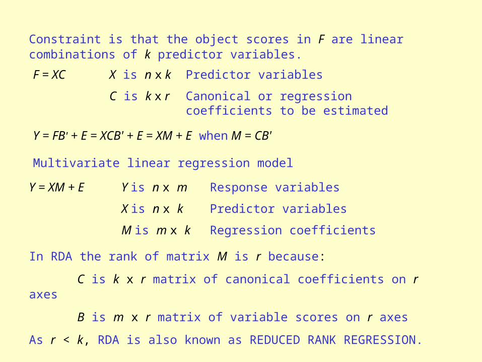
Constraint is that the object scores in F are linear combinations of k predictor variables.
F = XC X is n x k Predictor variables
C is k x r Canonical or regression coefficients to be estimated
Y = FB' + E = XCB' + E = XM + E when M = CB'
Multivariate linear regression model
Y = XM + E Y is n x m Response variables
X is n x k Predictor variables
M is m x k Regression coefficients
In RDA the rank of matrix M is r because:
C is k x r matrix of canonical coefficients on r axes
B is m x r matrix of variable scores on r axes
As r < k, RDA is also known as REDUCED RANK REGRESSION.

For designed experiments, treatments can be represented as DUMMY VARIABLES (0 blank, 1 treated).
Regression model is now ANALYSIS OF VARIANCE (ANOVA) and technique is MULTIVARIATE ANALYSIS OF VARIANCE (MANOVA). Can use RDA and associated permutation tests to assess statistical significance.
Advantages over conventional MANOVA
1) RDA can analyse any number of species, whereas in MANOVA and canonical correlation analysis, the number of species must be less than (n – k).
2) In MANOVA, standard statistical tests use tables to assess significance. Assume data are multivariate normally distributed. Permutation tests avoid this assumption.
Blocks can be used as covariables so as to eliminate their effects – partial MANOVA = multivariate analysis of covariance MANOCO.
Can also be used in analysis of BACI (Before-After-Control-Impact) data.
e.g. Liming experiment carried out in 3 forests; in each forest there are six plots, each recorded 4 times (one before, three after the treatment). Treatment is application of three doses of lime.

Model is:
y = plot effect + time effect + lime effect + error
Interested in lime effect. Partial out plot and time as covariables. For permutation tests, under the null hypothesis of no lime effect, only the plots within each forest are exchangeable with each other. Forests thus represent BLOCKS. Must have 3 forests as 3 dummy variables in covariables, i.e. covariables are 3 blocks, 4 times, 6 plots. Restricted permutation, condition permutations on the (3 – 1) + (4 – 1) independent block and time covariables.
Presentation of results
1) Distance biplot - emphasis on objects
2) Correlation biplot - emphasis on variables and predictor variables
3) Regression biplot - displays regression coefficients of multivariate multiple regression of variables and predictors
4) t-value biplot

REGRESSION BIPLOTSIf the number of predictor variables is small (< 10 say) and their mutual correlations not too high (< 0.6), can be useful to represent predictor variables by their canonical coefficients with axes. Coefficients are the weights of the predictor variables in the linear combination that defines a constrained ordination axis.
Canonical coefficients are coefficients of multiple regression of axis onto predictor variables. Extends from axes to response variables.
If use canonical coefficients, environmental variables with the response variables form a biplot of a table of multiple regressions for each of the species on the environmental variables.
Regression biplot represents the CONDITIONAL EFFECTS (multiple regression coefficients) of predictor variables (i.e. effects when other predictors are considered) whereas correlation biplot represents the MARGINAL EFFECTS (correlations) of predictor variables when considered singularly.
Note multiple regression coefficients can be unstable and unreliable if there are many predictor variables or if they have high mutual correlations. Take care to exclude predictors with VARIANCE INFLATION FACTORS > 20.


Baar & ter Braak (1996)

T-VALUE BIPLOTS
In regression analysis, results are not only regression coefficients but also their associated t-values. Can display t-values by changing the lengths of species arrows and environmental variable arrows. t-value biplot can be visualised as a weighted PCA of t-values.
Points for environmental variables can be projected on the arrow for a species. If the projection point falls on the head of the species arrow, approximated t-value is 2. If it falls on the other side of the origin, but at same distance, t-value is –2. If projection point falls closer to origin, t-value < 2; points further away > 2. Regression coefficients of the environmental variable are therefore significantly different from 0 (t-value of 2 is critical value at 5% level if degrees of freedom > 20).
Van Dobben circles – draw circle with diameter exactly equal to t-value of 2 for environmental variable of interest. All species inside circle are significantly positively correlated with that variable. Draw mirror-image of circle (dashed line) to show those species negatively correlated with that variable.


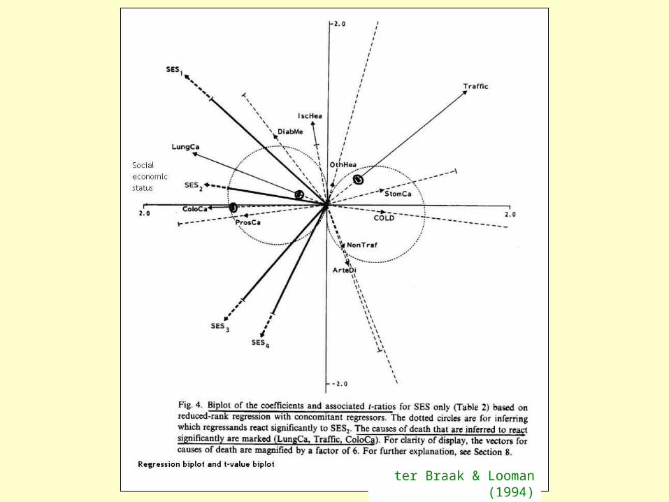
ter Braak & Looman (1994)

IMPACT OF SEASONAL SHEEP GRAZING ON FORMERLY FERTILISED
GRASSLAND
Watt T.A. et al. (1996) J. Vegetation Science 7, 535–542
Replicated sheep grazing experiment
2 x 2 x 2 factorial design
8 treatments assigned at random to areas 50 x 50m in each of two blocks
For each grazing period - winter
- summer
- spring
there are two levels of grazing
- sheep present or absent in winter
- sheep present or absent in spring
and two different sward heights
- short (3cm)
- tall (6 cm)


CLASSIFICATION EVALUATION

Dummy variable coding for groups corresponding to the competing cluster models.
Transect Two-group model
Consensus model Transition model
TWINSPAN model
1 1 0 0 1 0 0 1 0 1 0 0
2 0 1 0 0 1 0 0 1 0 0 1
3 0 1 0 0 1 0 1 0 0 0 1
4 1 0 1 0 0 1 0 0 1 0 0
5 1 0 1 0 0 1 0 0 1 0 0
6 1 0 1 0 0 1 0 0 1 0 0
7 0 1 0 0 1 0 1 0 0 1 0
8 1 0 1 0 0 1 0 0 1 0 0
9 1 0 1 0 0 1 0 0 1 0 0
10 0 1 0 0 1 0 0 1 0 0 1
11 1 0 0 1 0 0 1 0 0 1 0
12 0 1 0 0 1 0 0 1 0 0 1
13 0 1 0 0 1 0 0 1 0 0 1
14 0 1 0 0 1 0 0 1 0 0 1
15 0 1 0 0 1 0 0 1 0 0 1
16 1 0 0 1 0 1 0 0 1 0 0
17 1 0 0 1 0 1 0 0 0 1 0Y = + X + Z + Y = 17 transects x 210 species
X = two-group model (covariable) Z = three-group modelH0 = 0
- three-group model is statistically no better than the two-group at explaining variability in Y.
Partial Mantel test; partial CCA; partial RDARestricted permutations to occur among transects within groups of the two-group model in accordance with the null hypothesis of the existence of two groups.

Results of partial Mantel tests, partial CCA tests, and partial RDA tests to determine whether any of the proposed 3-group model provides a significantly better fit to the data than the 2-group model for explaining variability in the vegetation species data.
Model Mantel CCA RDA
F P F P F P
(a) All species
Consensus 4.042 0.009** 1.770 0.014* 2.828 0.005**
Transition 0.717 0.109 0.994 0.421 1.095 0.319
TWINSPAN 1.519 0.094 0.908 0.741 1.210 0.175
(B) Native species
Consensus 3.970 0.016* 1.746 0.004** 2.886 0.004**
Transition 0.309 0.379 1.013 0.404 1.089 0.331
TWINSPAN 0.815 0.207 0.911 0.679 1.058 0.339
Notes: P values were calculated using 999 permutations under the reduced model. Results are shown (a) for all species and (b) for native species only.* P < 0.05: ** P < 0.01

DATA DIVING WITH CROSS-VALIDATION:
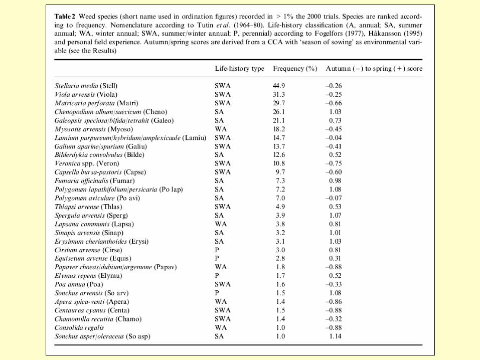
AN INVESTIGATION OF BROAD-SCALE GRADIENTS IN SWEDISH WEED COMMUNITIES
E. Hallgren, M.W. Palmer & P. Milberg (1999), Journal of Ecology 87:1037-1051
Flow chart for the sequence of analyses employed in the study. Solid lines represent the flow of data and dashed lines the flow of ideas or analyses.

Environmental variables used in the analyses
Nominal variables
Sowing season (autumn or spring)
Geographical regions: Swedish counties (A-H)
Soil types (1, sandy soil; 2, fine sand soil; 3, silty soil; 4, loamy soil; 5, silty clay loam; 6, heavy to very heavy clay soil; 7, organogenic soil)
Crop species (barley, wheat, rye, oats, turnip rape, rape; categorised according to season of sowing)
Interval-scale variables
Year of trial (1970.1994)
Organic content (%; seven categories)
Continuous variables
Nitrogen fetilization (N ha-1)
Crop yield (kg ha-1)
Map of Sweden with the
geographical regions (A-H)
indicated.
Data on weed species; 2824 field trials; 2090 with complete environmental data.
Split into 1000 exploratory data and 1000 confirmatory data

TECHNIQUES USED
1. Detrended correspondence analysis - reveal gradients in data
2. Canonical correspondence analysis - Monte Carlo permutation tests on "trace" statistic
3. Partial DCA - any interpretable species patterns beyond the effects of measured environmental variables
4. Partial CCA - can one set of variables explain variation in species composition not explained by a second set of variables
5. Stepwise CCA
Exploratory data set 1000 plots
Confirmatory data set 1000 plots
Display data set 2359 plots

Weed community related to SEASON OF SOWING, GEOGRAPHICAL REGION, Weed community related to SEASON OF SOWING, GEOGRAPHICAL REGION, SOIL TYPE, and CROP SPECIES. Also AUTUMN SOWN CROPS HAVE CHANGED SOIL TYPE, and CROP SPECIES. Also AUTUMN SOWN CROPS HAVE CHANGED OVER TIME.OVER TIME.

Autumn sown Spring sown

VARIANCE PARTITIONINGPartitioning of the explainable variable variation among the four groups of variables. TU is the variation described by T but not explained by U. TU is the variation jointly described by T and U. UT is the variation described by U but not by T.S = soil type; C = crop species; Y = year; G = geographical region
Percentage of explainable variation
Percentage of explainable variation
T U T|U TU U|T Other T U T|U TU U|T Other
Autumn
Spring
S G 28.6 9.4 33.9 28.2 S G 34.7 10.8 36.3 18.2
C SG 24.5 7.2 64.6 3.7 C SG 14.3 4.6 77.1 1.0
Y CSG 3.7* 2.4 93.9 - Y CSG 4.0* 4.2 91.9 -
S C 32.7 5.3 26.4 35.6 S C 43.4 2.0 16.9 37.6
S Y 36.4 1.6 4.5 57.5 S Y 45.3 0.17 8.0 46.6
C G 28.2 3.5 39.7 28.6 C G 14.9 4.0 43.1 38.0
C Y 29.0 2.7 3.3 65.0 C Y 14.9 4.0 4.2 77.0
G Y 42.5 0.78 5.3 51.5 G Y 46.1 1.0 7.1 45.8
Year – low Soil – high Geography - high

Autumn sown Spring sown

Autumn sown Spring sown

Autumn sown Spring sown


SHORT-TERM VEGETATION IN A FEN-MEADOW
ter Braak C.J.F. & Wiertz J. (1994) J. Vegetation Science 5, 361–372
20 plots in fen-meadow grassland 1977–1988


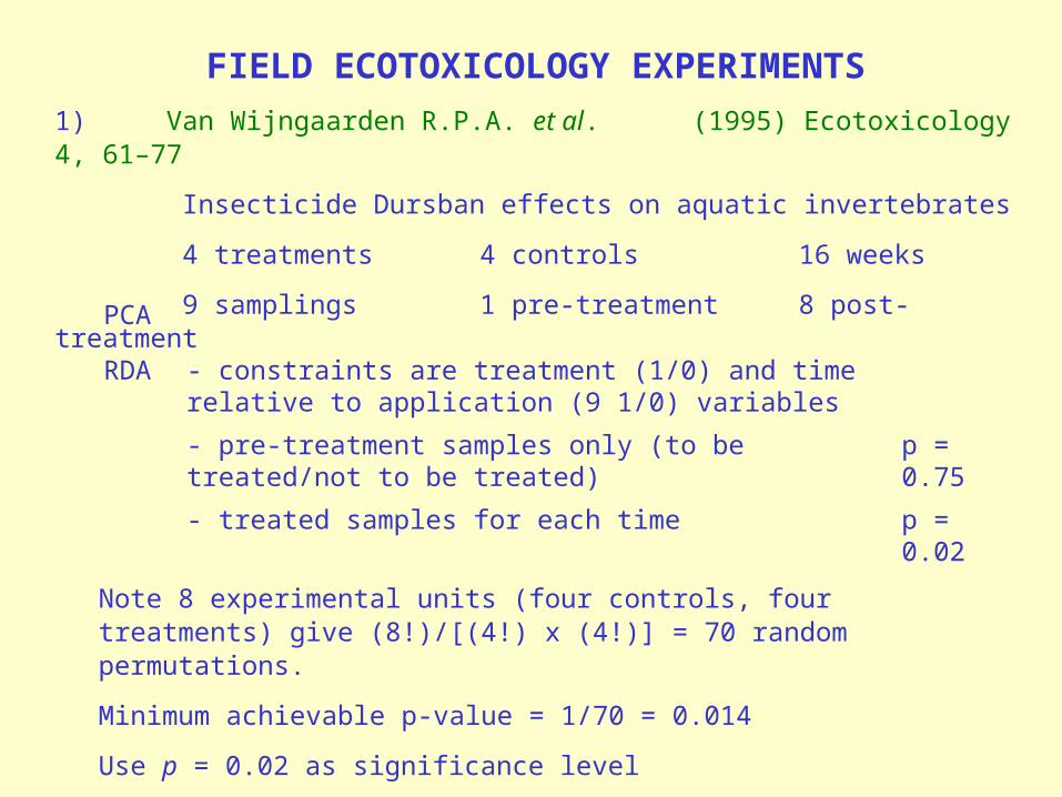
FIELD ECOTOXICOLOGY EXPERIMENTS
1) Van Wijngaarden R.P.A. et al. (1995) Ecotoxicology 4, 61–77
Insecticide Dursban effects on aquatic invertebrates
4 treatments 4 controls 16 weeks
9 samplings 1 pre-treatment 8 post-treatmentPCA
RDA - constraints are treatment (1/0) and time relative to application (9 1/0) variables
- pre-treatment samples only (to be treated/not to be treated)
p = 0.75
- treated samples for each time p = 0.02
Note 8 experimental units (four controls, four treatments) give (8!)/[(4!) x (4!)] = 70 random permutations.
Minimum achievable p-value = 1/70 = 0.014
Use p = 0.02 as significance level


RDA (redundancy analysis) biplot of species and centroids of contemporary samples in indoor microcosms. Centroids consist of contemporary samples in the replicates of the treatment and control microcosms (both N = 4). Centroids are shown as circles. Alphanumerical codes at centroids indicate treatment (T) or control (C) microcosms, followed by week of sampling relative to treatment date. Species are represented by species points.

2) Verdonschot & ter Braak (1994) Hydrobiologia 278, 251–266
Effects of chlorpyrifos on oligochaete communities
12 ditches BACI (before-after-control-impact) effect of insecticide
12 ditches with insecticide or control
8 ditches with insecticide, control or P or P/N addition (eutrophication)
MODEL y = ditch + time + chlorpyrifos + eutrophication + error
treatment(Partial) RDA used for anaylsis


PERMUTATION TEST
Ditches were randomised between treatments. Can permute ditches, not individual samples. Restricted permutations of ditches (‘plots’).
1) Control vs treated p < 0.01
*
i.e. Differences between control and treatment
2) Control vs treated, time as covariable p < 0.01
*
3) Treatment with chlorpyrifos
covariable p
Model ditch and chlorpyrifos
time 0.03 *
chlorpyrifos ditch and time 0.18 ns
4) Eutrophication
Model P + P/N time 0.01 *
5) Ditch type
Clay type and eutrophication
time 0.01 *
Sand type and eutrophication
time 0.11 ns

FURTHER EXAMPLES OF HYPOTHESIS TESTING USING CONSTRAINED
ORDINATIONS AND PERMUTATION TESTS
ECOLOGY
Odland A., Birks H.H., Botnen A., Tønsberg T., & Vevle O.
(1991) Regulated Rivers: Research & Management 6, 147-162 (Effects of water withdrawal on bryophytes and lichens at waterfalls)
Leps J. & Hadincova V. (1992) J. Vegetation Science 3, 119-124 (Reliability tests of vegetation analysis)
Leps J. et al. (1995) J. Vegetation Science 6, 37-42 (Field experiments on goat grazing)
van den Brink P.J. et al. (1996) Environmental Toxicology & Chemistry 15, 1143-1153 (Effects of Durspan on invertebrates)
Baar J. & ter Braak C.J.F.
(1996) Applied Soil Ecology 4, 61-73 (Effects of litter and humus type on fungal sporocamps)

PALAEOECOLOGY
Anderson N.J., Renberg I. & Segerström U.
(1995)
J. Ecology 83, 809-822 (Influence of land-use on diatom assemblages and productivity)
Odgaard B.V. (1992)
The Holocene 2, 218-226 (Charcoal-pollen relationships in lake sediments)
Anderson N.J., Odgaard B. V., Segerström U. & Renberg I.
(1996)
Global Change Biology 2, 399-405 (Influence of recent climate change on diatom diversity and of land-use on diatom assemblages)

OTHER NUMERICAL TOOLS FOR TESTING ECOLOGICAL MULTIVARIATE
HYPOTHESES
1. Principal response curves - analysis of repeated measurement design to test and display treatment effects that change across time. Allows focus on time-dependent treatment effects. Test with model-based permutation tests.
Can also be used for effects that change across space.
2. Partial constrained ordinations, variance decomposition, and model-based permutation tests.
3. Distance-based redundancy analysis and generalised distance-based multivariate analysis of a linear model with model-based permutation tests.
4. Canonical analysis of principal co-ordinates.
5. Non-parametric analysis of variance with model-based permutation tests.
6. Multiple regression with model-based permutation tests.

TYPES OF GRADIENT ANALYSIS METHODS BASED ON WEIGHTED
AVERAGING
Community data - incidences (1/0) or abundances ( 0) of species at sites.
Environmental data - quantitative and/or qualitative (1/0) variables at same sites.
Use weighted averages of species scores (appropriate for unimodal biological data) and linear combinations (weighted sums) of environmental variables (appropriate for linear environmental data)

Method Abbreviation
Response variables (y)
Predictors (x)
Lecture
Correspondence analysis
CA (also DCA)
Community data
- 6
Canonical correspondence analysis
CCA (also DCCA)
Community data
Environmental variables
7
CCA partial least squares
CCA-PLSCommunity data
Many environmental variables
11
Weighted averaging calibration
WAEnvironmental variable
Community data
8
WA partial least squares
WA-PLSEnvironmental variable(s)
Community data
8
Co-correspondence analysis
CO-CACommunity data
Community data
11
Also partial CA, partial DCA, partial CCA, partial DCCA.

CCA-PARTIAL LEAST SQUARES (CCA-PLS)
Partial least squares (PLS) is a form of multivariate linear regression, popular in chemometrics, to handle large numbers of predictor variables without much loss of predictive power. PLS axes maximise covariance between predictors and response variable(s) under linear response model.
WA-PLS axes maximise covariance between weighted averages of predictors (e.g. species data) and response variable(s) under a unimodal response model to predict environmental variable(s) ('response variable(s)').
CCA-PLS combines best of PLS and CCA to predict species data from environmental data under the assumption that species respond to their environment (cf. WA-PLS). PLS selects linear combinations of species variables with certain optimal properties; CCA-PLS uses weighted averages with certain optimal properties. Can handle large numbers of predictor variables and maximises the covariance between weighted average species scores (responses) and linear combinations of the predictor, environmental variables.
First CCA-PLS component is linear combination of environmental data with maximum covariance with the weighted averages of the species data. Second and subsequent axes maximise this covariance with the constraint that the site scores are uncorrelated to previous site scores. Like CCA but with PLS's special approach of guarding against high correlations (multicollinearity) in the environmental variables.

ter Braak & Schaffers (2004) Ecology 85: 834-846
Problems: are carabid beetles in grassland more closely related to vegetation structure
(height, cover, biomass, etc.) than to vegetation composition?
Are fen bryophytes more closely related to vegetation composition than to water chemistry?
Data - beetles, plants, vegetation type, vegetation structure, and environmental variables
all from same set of sites.
Approaches
(1) RDA/CCA - predict beetles from environmental data.
- cannot predict beetles from vegetation data because may be more plant species (predictors) than sites. No constraints.
(2) CA/DCA of beetles and plants separately, correlate the axes (compare with Procrustes rotation). Correlative rather than predictive approach.
Can reduce plant data to (D)CA axes first, use these as predictors. Will work if major patterns in one biological data are important for the other response data-set. Need not be so.
(3) CCA-PLS - use linear combinations (weighted sums) of predictors. Not appropriate with biological predictors.
Need a one-step method where the most important relationships are expressed in the first
few axes so that nothing important is missed. Co-correspondence analysis.
CO-CORRESPONDENCE ANALYSIS (CO-CA)

CO-CORRESPONDENCE ANALYSIS (CO-CA) cont.Co-correspondence analysis (CO-CA)
Problem with combined CA is that each CA has its own site weights (the site's total abundance of the species in the analysis). Pointless to have weights that are a sum of both beetles and plants.
As in CA (reciprocal averaging algorithm) but has an explicit maximisation criterion for CO-CA, the covariance between WA species and site scores of beetles should be maximised with WA species and site scores of plant data. Replaces linear combinations (PCA, PLS, RDA) with weighted averages, so it is suitable for unimodal biological data.
Symmetric, descriptive CO-CA (can swap data sets)
Asymmetric, predictive CO-CA (data A are thought to influence data B)
CA - selects species scores (by WA) to maximise variance of site scores under the constraint that the species scores have unit variance. Symmetrical in that species and sites can be interchanged in the optimisation criterion.
CO-CA - calculates two sets of WA species and site scores to maximise weighted covariance between the two sets of WA species and site scores with allowance for differences in weights among data. What is maximised is covariance between two sets of site scores with common site weights; covariance is maximised by finding appropriate species weights. Species scores of one set are weighted averages of other set's site scores and site scores are weighted averages of the species scores of own set.
MATLAB, R

CO-CORRESPONDENCE ANALYSIS (CO-CA) cont.
Beetles 91 species, 173 plant species, 30 sites.
Eigenvalues of the first three axes of separate CAs and DCAs and of symmetric CO-CA of beetles and plants.
Axis
Method 1 2 3
Beetles
CA 0.50 0.36 0.32 4.99
DCA 0.50 0.32 0.21
Length of gradient 3.22 2.74 2.57
Plants
CA 0.57 0.53 0.42 5.65
DCA 0.57 0.41 0.27
Length of gradient 3.44 2.99 2.88
Beetles-plants CO-CA 0.25 0.13 0.08 0.94
Highly structured data-sets - high eigenvalues, long gradients.

Correlation coefficients between beetle-derived and plant-derived site scores of the first three axes of separate CAs and DCAs and of symmetric CO-CA (% fit = the percentage fit of the beetle data by the first two plant-derived axes).
Method Axis % fit (2 axes)
1 2 3
CA 0.88 0.27 0.46 15
DCA 0.89 0.53 0.07 16
CO-CA 0.96 0.94 0.88 19
Highest correlations for all three axes in CO-CA
Percentage variance for 2 axes highest (19%) in CO-CA

CO-CA biplots - centroid and biplot rules
Beetles Plants
Axes 1 & 2CCA beetles (91 species) - vegetation units (8 vars)19%CCA beetles - environment (13 vars) 18%CCA beetles - vegetation structure (9 vars) 13%CO-CA beetles - vegetation composition (173 vars)19%
Permutation testsCCA vegetation units 2 axes (P = 0.002, 0.01)CCA environment 2 axes (P = 0.001, 0.038)CCA veg. structure 2 axes (P > 0.30)CO-CA 2 axes P < 0.001 3 or later (P > 0.60)

CO-CORRESPONDENCE ANALYSIS (CO-CA) cont.
Need to know how many axes to consider for predictive CO-CA. Find optimal dimensions.
Leave-one-out cross-validation to find 'optimal' number of axes for prediction. Predict response species for the site left-out.
2 axes CO-CA plants predict 7.8% of beetle variance, vegetation units 8.1% (CCA), environmental variables 4.8% (CCA or CCA-PLS), and vegetation structure (CCA or CCA-PLS) negative fit.
Vegetation composition or vegetation units predict beetle composition better than environmental variables. Vegetation structure has no predictive value.
Veg units CCA
Env CCA-PLS
Struct CCA-PLS
Struct CCA
Plants CO-CA
Env CCA

CO-CORRESPONDENCE ANALYSIS (CO-CA) cont.
Direct ordination procedure for relating one community data-set to another community data-set.
Combines WA and PLS to maximise covariance between WA species scores of one community data-set with those of another. Finds ecological gradients common to both. Integrates WA-PLS and CCA-PLS with CCA, and brings 'biology' of one data-set into ordination procedures in a direct way.
Species assemblages are a multivariate 'bio-assay' of the environment. Assemblages analysed by CO-CA often give better predictions of another set of assemblages than using environmental variables alone. Often environmental basis for ecological gradients is not precisely known.
Fen bryophytes - vascular plants 28% explained CO-CA
Fen bryophytes - environmental variables 17%
CO-CA can be used to find good indicators for biodiversity. Not all species groups are equally easy to sample or identify. Can try to predict a 'difficult' group from an 'easy' group. Need representative full data for both species groups from common set of sites for CO-CA. After this, only the 'easy' group need be sampled. Another idea is to look at biological data at different taxonomic levels - species, genera, families, or as functional types. See how well each predicts each other.

CO-INERTIA ANALYSIS (Co-IA)
Doledec & Chessel (1994) Freshwater Biology 31: 277-294
Dray et al. (2003) Ecology 84: 3078-3089
Method for analysing species-environment data with many species and many environmental variables. Avoids multicollinearity problems and problems of CCA and RDA when there are more environmental variables than samples.
Analyses species-environment tables, and attempts to find new axes in both so that the covariance between the new sets of scores is maximised (as in PLS). The maximised covariance means a maximal correlation and maximal standard deviations of the new environmental and species scores.
First Co-IA axis identical to that of CCA-PLS.
In contrast to CCA and PLS, treats species and environmental data symmetrically (no responses or predictors). Analyses covariation only, no regression models or prediction models are involved.
Species data Environmental data
CCA Part CA (unimodal) Part multiple regression
Co-IA Part CA (unimodal Part PCAor part PCA (linear)
R

Co-inertia analysis as an extension of the initial approach of Tucker (1958), which was performed in connecting two standardised principal component analyses (the upper arrows symbolise the initial transformation of raw data, i.e. centring, double centring, etc.). Let X be the environmental array. Let Y be the faunistic array. Samples n1 and n2 are two given stands that are to be projected on both the environment axis and the fauna axis of the co-inertia analysis. These projections define new scores of stands that are the most covariant, i.e. these new scores have a maximal correlation and the standard deviations of the new scores are maximal.
CO-INERTIA ANALYSIS (Co-IA) cont.

CO-INERTIA ANALYSIS (Co-IA) cont.
Co-IA Separate PCAs Co-IA
AxesVarEnv on Co-IA axes
VarBio on Co-IA axes
Env Biology R
1 5.23 23.66 5.34 25.26 0.93
2 0.96 12.35 1.54 14.66 0.86
[16 ponds, 91 taxa, 11 environmental variables]
From Co-IA ordination plots, can infer species weighted averages (CA) or weighted sums (PCA) and relative class totals, and less about the other 8 tables potentially present in the analysis of species-environmental data.
The more members a group of correlated environmental variables contains, the more that group is emphasized. Group size has less influence in CCA or CCA-PLS.
General method to relate any kinds of data using any kind of analysis (PCA, CA, multiple correspondence analysis) or between-class and within-class analyses.

CO-INERTIA ANALYSIS (Co-IA) cont.
Co-inertia – global measure of co-structure of sites in two hyperspaces (e.g. species x sites, environment variables x sites).
High when two structures vary simultaneously (and also when they vary inversely).
Low when they vary independently or do not vary.
Inertia is sum of variances; co-inertia is a sum of square covariances.

Square covariance or co-inertia can be decomposed into
a) correlation
b) variance of sites in species data (Y)
c) variance of sites in environmental data
(X)

Canonical correlation analysis
Maximises square correlation
CCA or RDA Maximises the product of the square correlation by the species variance, i.e. the variance explained by X. Hence possible to do variance partitioning
Co-inertia analysis Maximises square covariance
Canonical correlation analysis is defined by two Mahalanobis metrics (X'DX)-1 and (Y'DY)-1; CCA and RDA has only Mahalanobis metric (X'DX)-1; co-inertia has none (D = diagonal matrix of site weights).
Mahalanobis metric takes into account correlation within the data and involves the inverse of the variance-covariance matrix X and/or Y. Results in dimensional constraints.

Method Constraints
Canonical correlation analysis
Number of species + number of environmental variables < number of sites
CCA or RDA Number of environmental variables < number of sites
Co-inertia analysis No constraints but sites in Y and X must be weighted the same way for the analysis
Co-inertia analysis similar to CanCor and CCA but has fewer constraints
Co-inertia analysis can use any distance measure, not just Euclidean or chi-squared distances.

Co-inertia analysis can be extended from (a) Y and X to
(b) Principal co-ordinates of Y and X
(c) RLQ analysis (Y, X, species traits)
(d) Multiple co-inertia analysis to link k tables measuring k sets of variables through time for the same sites
(e) Concordance analysis to link k tables to a reference table
(f) Between-class or within-class co-inertia analysis to study species-environment relationships according to groups of sites
(g) STATICO – k pairs of tables (Y and X) through time (Thioulouse et al. (2004) Ecology 85: 272-283)

PROTEST - A Procrustes randomisation test
Jackson (1995) Ecoscience 2, 297-303
Peres-Neto & Jackson (2001) Oecologia 129, 169-178
Procrustes rotation - matrices of species data and environmental data. Ordinate each separately, compare ordinations by Procrustes analysis - rigid rotation, translation, reflection, and dilation to minimise the sum of squared residual deviations between points for each observation. Estimate m2, the goodness-of-fit or concordance measure between two ordinations or two matrices.

PROTEST - randomise one matrix so that each site can assume any of the possible values for a given variable, but values are not inter-changed among variables, i.e. within-matrix covariance structure is not changed. Calculate m2 for randomised data, repeat many times, Compare observed m2 with the values based on randomised data, to test if observed m2 is greater than expected under random inter-matrix association.
19 lakes - benthic invertebrates, water chemistry, geography, and morphology.
m2 pInvertebrates - geography 0.722 0.020 *Chemistry - geography 0.805 0.110Morphology - geography 0.796 0.108Invertebrates - chemistry 0.720 0.021 *Invertebrates - morphology 0.858 0.330
www.zoo.utoronto.ca/jackson/software
PROTESTR

PROCRUSTEAN CO-INERTIA ANALYSIS
Dray et al. (2003) Ecoscience 10, 110-119
Provides a means not only of calculating m2, the concordance, between two ordinations but also of providing a graphical representation of this concordance.
Co-inertia analysis - general symmetric method of comparing X and Y by finding scores in both X and Y space with maximum covariance. Maximises variance in X and Y simultaneously.
Procrustes co-inertia analysis provides common graphical representation of X and Y in same, common space.
PROTEST - permutation test for Procrustes analysis. Test hypothesis of no link between X and Y against hypothesis that there is a common structure.
Procrustean co-inertia analysis not restricted to Euclidean or chi-squared metrics. Can use any distance measure, express as principal co-ordinates, and then do Procrustean co-inertia analysis and PROTEST.
R

INCORPORATION OF ECOLOGICAL KNOWLEDGE ABOUT SPECIES IN
CONSTRAINED ORDINATIONSMatching species traits to environmental
variables
Three-table ordination - RLQ method
Dolédec et al. (1996) Env. Ecol. Stat. 3; 143-166.
R L (link) Q
Env. variables
Sites R
Sites
Species
L
QSpecies
Traits
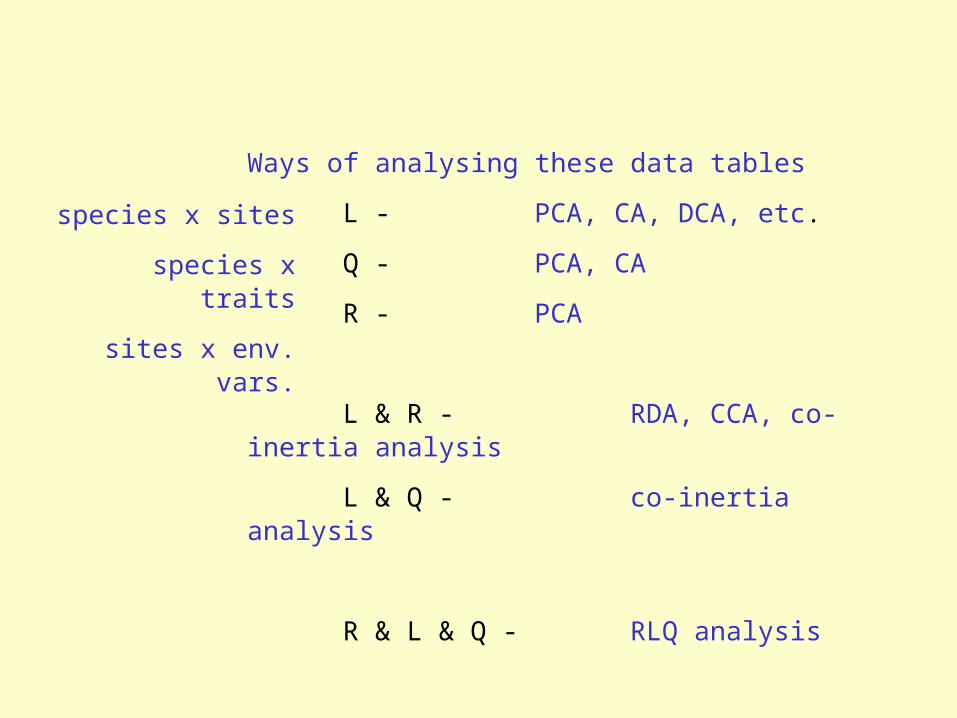
Ways of analysing these data tables
L - PCA, CA, DCA, etc.
Q - PCA, CA
R - PCA
L & R - RDA, CCA, co-inertia analysis
L & Q - co-inertia analysis
R & L & Q - RLQ analysis
species x sites
species x traits
sites x env. vars.

Matching species traits or ecological indicator values to environmental variables.
Simple summary
• Treat each observed individual in the species data as a new unit (row in the new data matrix).
y = trait or indicator value of the individual.
x = environmental data of the site where individual occurs.
• Apply RDA of y with respect to x.
Rationale
• This is precisely CA with linear regression constraints on both rows and columns.
Uses co-inertia analysis. Could use PLS instead.
• Maximises the covariance between linear combinations of columns of matrices R (environmental variables) and Q (species traits).
ADE-4 (R)

R 51 sites x 11 environmental variables
L 51 sites x 40 species
Q 4 traits x 40 species (feeding habit, feeding stratum, breeding stratum, migratory strategy)
Example - bird assemblages along urban-
rural gradient
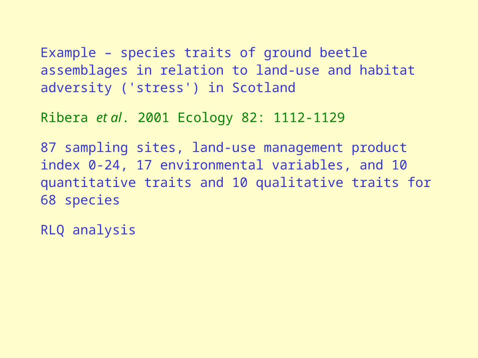
Example – species traits of ground beetle assemblages in relation to land-use and habitat adversity ('stress') in Scotland
Ribera et al. 2001 Ecology 82: 1112-1129
87 sampling sites, land-use management product index 0-24, 17 environmental variables, and 10 quantitative traits and 10 qualitative traits for 68 species
RLQ analysis

Quantitative traits
Qualitative traits
variance variance
Habitat Traits Habitat Traits
RLQ axis 1 7.50 1.39 7.30 0.16
PCA axis 1 7.72 3.17 7.72 0.32
% potential variability explained by RLQ axis 1
97.1% 42.8% 94.6% 50%
Total variance RLQ axis 1
84.8% 90.2%
P (Monte Carlo) <0.001 <0.001

First ordination axis of the RLQ analysis of the quantitative species traits: (a) scores of the sites (each vertical line stands for a site, and arrows separate main types of land-use [1, upland or very wet grassland, heather, bare peat; 2, rough or wet grass, extensive pastures, gorse, coniferous forest, recently burnt heather; 3, grassland; 4, set aside and forage rape; 5, cultivated fields]); and (b) position of species at the average score of the sites in which they occur.
Ribera et al. 2001

First ordination axis of the RLQ analysis of the qualitative species traits: (a) scores of the sites, (b) position of species at the average score of the sites in which they occur (vertical line), and (c) position of the qualitative traits at the average score of the species in which each of the modalities occur (circles).
Ribera et al. 2001

Conclusions:
1. First environmental axis very strong. Negatively related to land-use intensity and positively related to increasing elevation and habitat diversity.
2. In highly managed lowland sites, ground beetles were smaller and frequency of species with good dispersal abilities was high.
3. In lowland sites, species have broader bodies, longer trochanters, and wider femora (associated with plant eaters), paler in colour, overwintered only as adults, bred in spring or autumn, and were active in summer.
4. In upland sites, opposite species traits.
5. Suggests existence of functional groups of species and traits associated with different habitats.
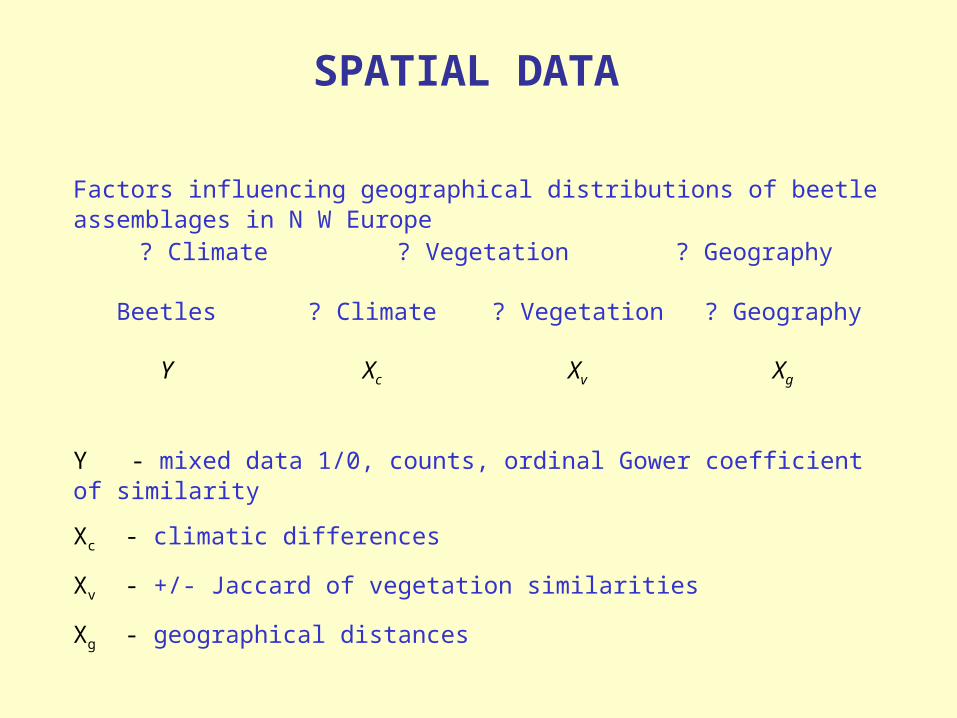
SPATIAL DATA
Factors influencing geographical distributions of beetle assemblages in N W Europe
? Climate ? Vegetation ? Geography
Beetles ? Climate ? Vegetation ? Geography
Y Xc Xv Xg
Y - mixed data 1/0, counts, ordinal Gower coefficient of similarity
Xc - climatic differences
Xv - +/- Jaccard of vegetation similarities
Xg - geographical distances

MANTEL TEST
Matrix correlation Y and Xg
Standardise matrices r and Z = yijxij/m
How to assess value of r or Z?
Randomise order in Y, recalculate r many times, compare r with randomised r.
How to justify this?
1) Mechanism that generates Y distances independent of mechanism that generates Xg.
2) Random sampling argument Y independent of Xg.
For n = 9, there are 9! possible permutations = 362880
999, 4999, 9999 randomisations.
Find significant r for Y and Xg, Y and Xv, and Y and Xc.
Which is important?R

PARTIAL MANTEL TEST ( partial regression)
Y Control for geography Xg Xc
Y Control for geography Xg Xv
(covariables)Compute matrix X1
c that contains residuals of linear regression of Xc on
Xg.
Compute matrix X1v that contains residuals of linear regression of Xv on
Xg.
Do Mantel tests using X1c and Y and X1
v and Y.
Partial tests with up to 9 explanatory or covariable matrices.
Jean & Bouchard (1991) Landscape data and GIS
Brown et al. (1991) Colour patterns of lizards on Tenerife and Canaria
* Lush/arid habitat hypothesisAltitude hypothesisGeographical proximity hypothesis
Empirical modelling in presence of spatial autocorrelation
Legendre & Troussellier (1988) Limnol. & Ocean. 33, 1055–67Borcard et al. (1992) Ecology 73, 1045–1055


SPATIAL AND TEMPORAL DATASpace-time patterns
Turner & Hodgson (1983) Journal of Ecology 71, 95–118
Pollen data 38 sites in N Pennines zone Vlla ‘Atlantic’
228 samples
1) Any significant temporal changes?
2) Any significant between-site spatial variation?
Besag & Diggle (1977) Monte Carlo tests
1) Site heterogeneity. 31 sites showed temporal change in tree and shrub pollen, 12 showed changes in herb pollen.
2) Between-site variation mean frequencies at each site. Assigned randomly 228 samples to 38 sites, each equal size to original. Calculate between-site statistics, repeat many times. Trees and shrubs – spatial pattern significant, also herb pollen.
Then tried to explain variation in relation to E, N, altitude, topography, bedrock. Multicollinearty.

Partial constrained ordinations
Pollen data Explan. variable Test
Y Depth Temporal varn
Y Site membership Spatial varn
Variance partitioning into spatial component, temporal component, spatial when time allowed for, temporal variation when space allowed for. Permutation tests.
Individual pollen types
RESPONSE VARIABLE
COVARIABLES EXPLANATORY VARIABLES
e.g. Pinus x and y co-ordinates
Altitude, topography, bedrock
Partition variance into Ecology independent of geography
Geography independent of ecology
Geographically covarying ecology
Unexplained variancei.e. (partial) multiple regression with permutation tests

IMPACT TO QUATERNARY PALAEOECOLOGY
Descriptive phase - patterns are detected, described and classified
Narrative phase - plausible, inductively-based explanations, generalisations, or reconstructions are proposed for observed patterns
Analytical phase - falsifiable or testable hypotheses are proposed, evaluated, tested and rejected
Why is there so little analytical hypothesis-testing in palaeoecology?
MONTE CARLO PERMUTATION TESTS are valid without random samples, can be developed to take account of the properties of the data of interest, can use "non-standard" test statistics, and are completely specific to the data-set at hand. Ideal for palaeoecology.
1. This is a worthless nonsense.2. This is an interesting, but perverse point of view.3. This is true but quite unimportant.4. I have always said so.
A WARNINGWith the right type of observation, experimentation, and attempts at falsification, hypothesis can be solidified into ecological theories. J.B.S. Haldane (1963) has observed, rather cynically, that this process is normally reflected in four stages through which the hypothesis passes in the regard of the scientific community:

MAJOR PLAYERS IN HYPOTHESIS TESTING USING PERMUTATION TESTS
Bryan F.J. Manly 1991
Pierre Legendr
e 1998
Marti J. Anderson 2001
Cajo J.F. ter
Braak 1992