J. Roychowdhury, University of California at Berkeley Slide 1

Numerical Algorithms for ODEs/DAEs(Transient Analysis)

J. Roychowdhury, University of California at Berkeley Slide 2

Solving Differential Equation Systems

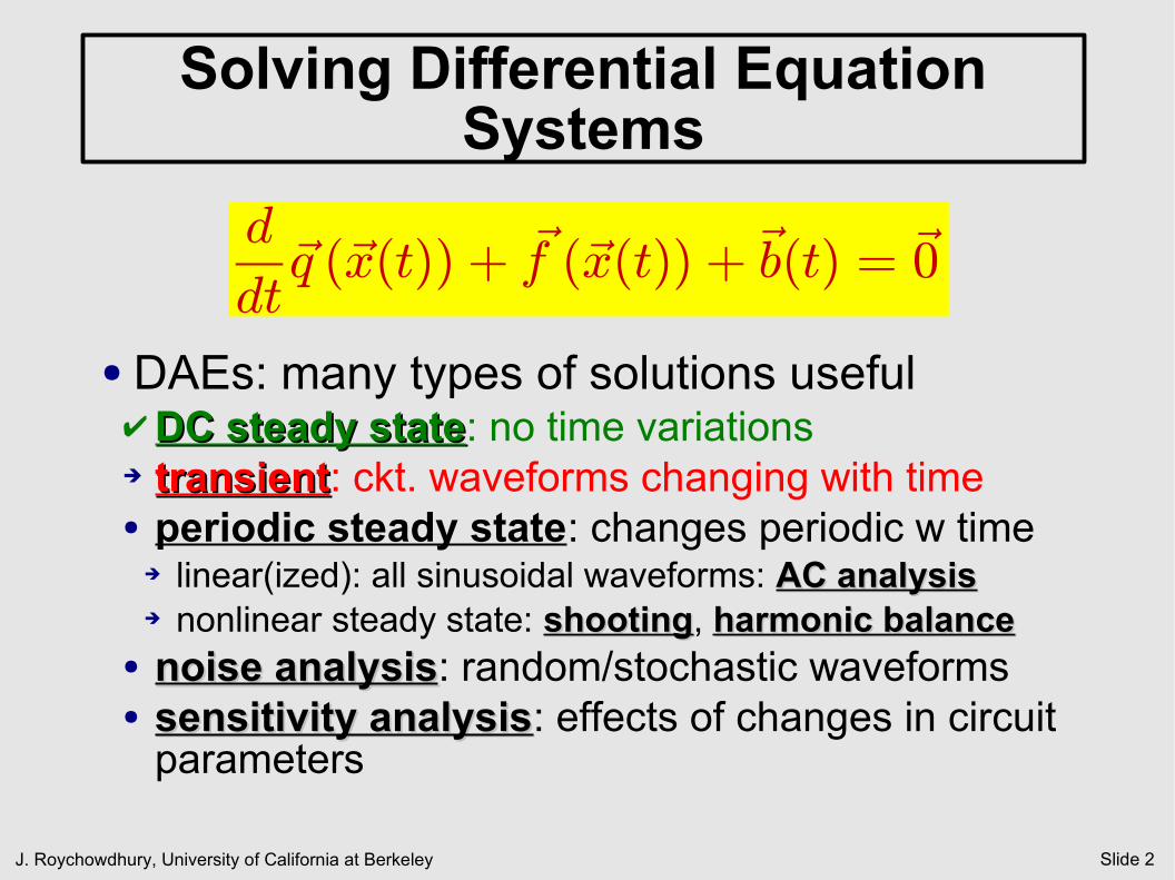
● DAEs: many types of solutions useful DC steady stateDC steady state: no time variations➔ transienttransient: ckt. waveforms changing with time● periodic steady state: changes periodic w time

➔ linear(ized): all sinusoidal waveforms: AC analysisAC analysis➔ nonlinear steady state: shootingshooting, harmonic balanceharmonic balance

● noise analysisnoise analysis: random/stochastic waveforms● sensitivity analysissensitivity analysis: effects of changes in circuit

parameters

d

dt~q (~x(t)) + ~f (~x(t)) +~b(t) = ~0

J. Roychowdhury, University of California at Berkeley Slide 3

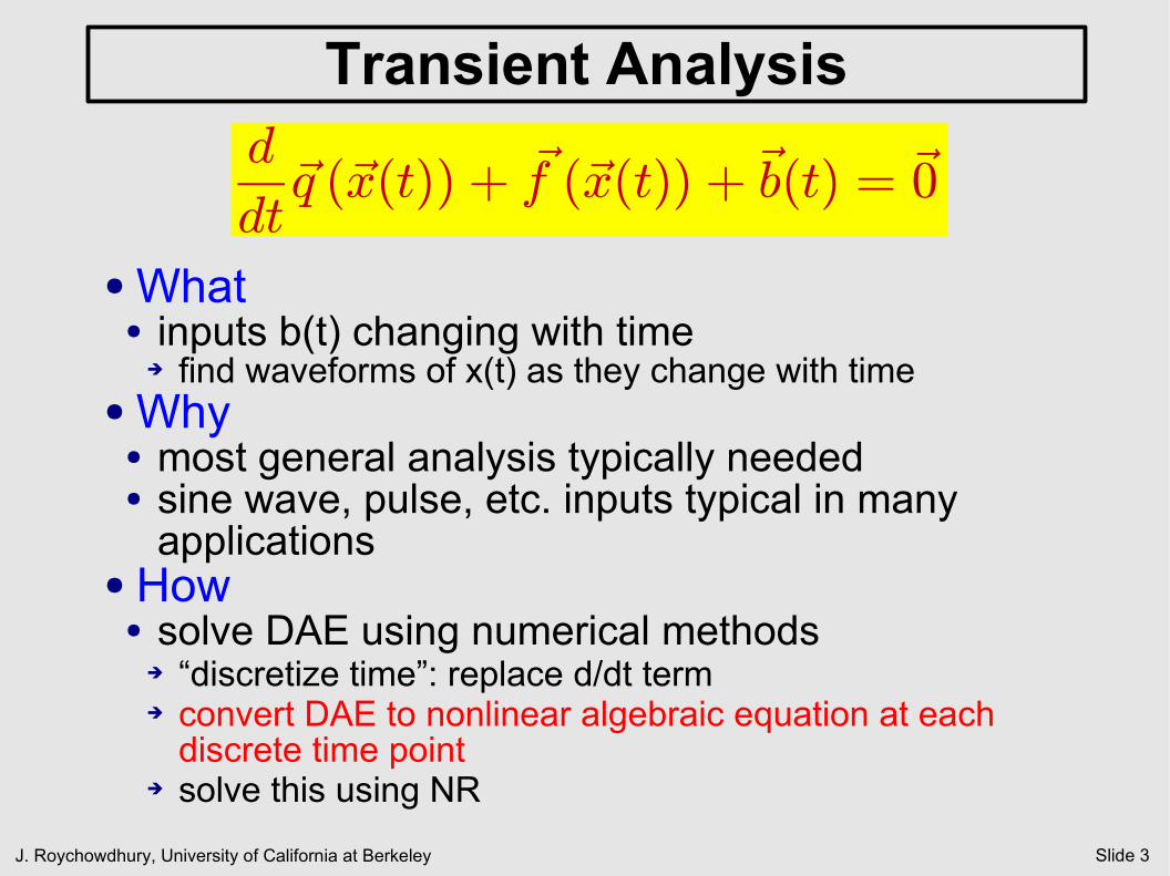
Transient Analysisd

dt~q (~x(t)) + ~f (~x(t)) +~b(t) = ~0

● What● inputs b(t) changing with time

➔ find waveforms of x(t) as they change with time● Why

● most general analysis typically needed● sine wave, pulse, etc. inputs typical in many

applications● How

● solve DAE using numerical methods➔ “discretize time”: replace d/dt term➔ convert DAE to nonlinear algebraic equation at each

discrete time point➔ solve this using NR

J. Roychowdhury, University of California at Berkeley Slide 4

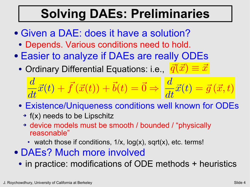
Solving DAEs: Preliminaries● Given a DAE: does it have a solution?

● Depends. Various conditions need to hold.● Easier to analyze if DAEs are really ODEs

● Ordinary Differential Equations: i.e.,

● Existence/Uniqueness conditions well known for ODEs➔ f(x) needs to be Lipschitz➔ device models must be smooth / bounded / “physically

reasonable”● watch those if conditions, 1/x, log(x), sqrt(x), etc. terms!

● DAEs? Much more involved● in practice: modifications of ODE methods + heuristics

~q(~x) ´ ~xd

dt~x(t) = ~g (~x; t)

d

dt~x(t) + ~f (~x(t)) +~b(t) = ~0)

J. Roychowdhury, University of California at Berkeley Slide 5

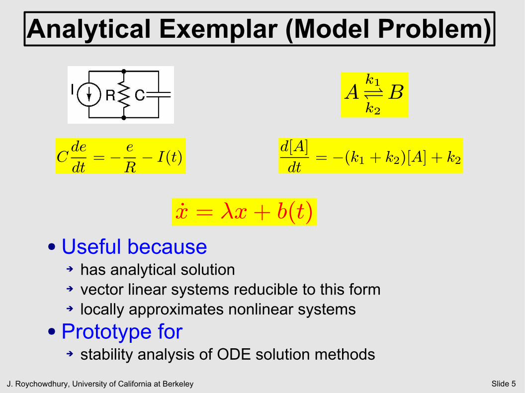
Analytical Exemplar (Model Problem)

● Useful because➔ has analytical solution➔ vector linear systems reducible to this form➔ locally approximates nonlinear systems

● Prototype for➔ stability analysis of ODE solution methods

Ak1­k2B

Cde

dt= ¡ e

R¡ I(t) d[A]

dt= ¡(k1 + k2)[A] + k2

_x = ¸x+ b(t)

J. Roychowdhury, University of California at Berkeley Slide 6

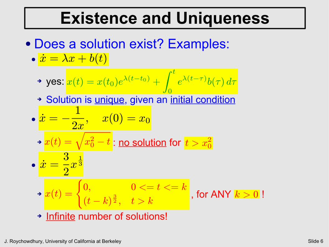
Existence and Uniqueness● Does a solution exist? Examples:

●

➔ yes:

➔ Solution is unique, given an initial condition

●

➔ : no solution for

●

➔ , for ANY !

➔ Infinite number of solutions!

x(t) = x(t0)e¸(t¡t0) +

Z t

0

e¸(t¡¿)b(¿) d¿

_x = ¸x+ b(t)

_x = ¡ 1

2x; x(0) = x0

x(t) =qx20 ¡ t t > x20

_x =3

2x13

k > 0x(t) =

(0; 0 <= t <= k

(t¡ k) 32 ; t > k

J. Roychowdhury, University of California at Berkeley Slide 7

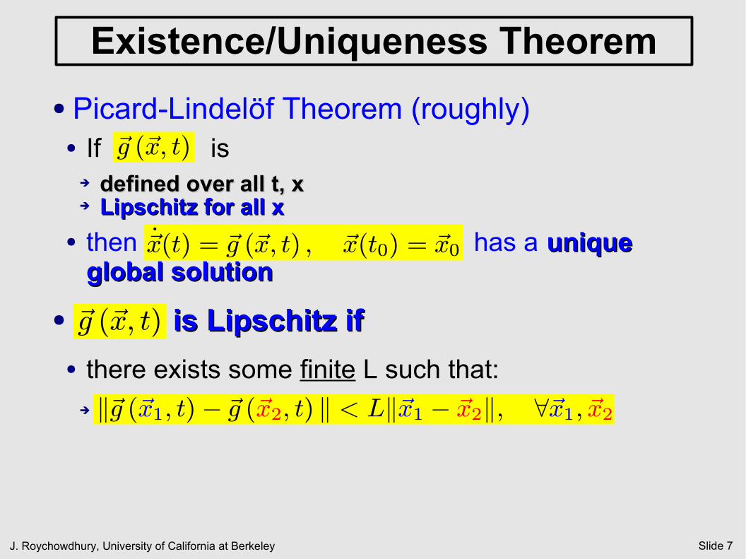
Existence/Uniqueness Theorem

● Picard-Lindelöf Theorem (roughly)● If is

➔ defined over all t, xdefined over all t, x➔ Lipschitz for all xLipschitz for all x

● then has a unique unique global solutionglobal solution

● is Lipschitz ifis Lipschitz if

● there exists some finite L such that:➔

~g (~x; t)

_~x(t) = ~g (~x; t) ; ~x(t0) = ~x0

~g (~x; t)

k~g (~x1; t)¡ ~g (~x2; t) k < Lk~x1 ¡ ~x2k; 8~x1; ~x2

J. Roychowdhury, University of California at Berkeley Slide 8

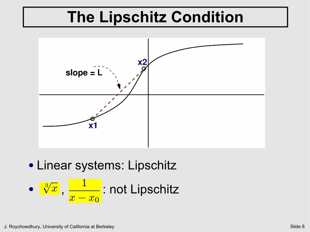
The Lipschitz Condition

● Linear systems: Lipschitz

● , : not Lipschitz3px 1

x¡ x0

J. Roychowdhury, University of California at Berkeley Slide 9

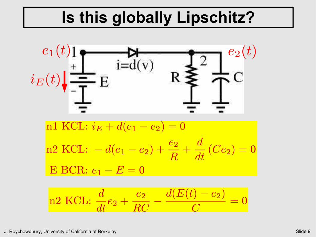
Is this globally Lipschitz?

e1(t) e2(t)

iE(t)

n1 KCL: iE + d(e1 ¡ e2) = 0

n2 KCL: ¡ d(e1 ¡ e2) +e2R+d

dt(Ce2) = 0

E BCR: e1 ¡E = 0

n2 KCL:d

dte2 +

e2RC

¡ d(E(t) ¡ e2)C

= 0

J. Roychowdhury, University of California at Berkeley Slide 10

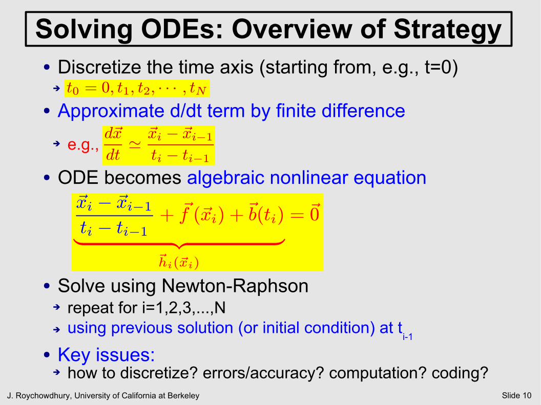
Solving ODEs: Overview of Strategy● Discretize the time axis (starting from, e.g., t=0)

➔

● Approximate d/dt term by finite difference

➔ e.g.,

● ODE becomes algebraic nonlinear equation

● Solve using Newton-Raphson➔ repeat for i=1,2,3,...,N➔ using previous solution (or initial condition) at t

i-1

● Key issues:➔ how to discretize? errors/accuracy? computation? coding?

t0 = 0; t1; t2; ¢ ¢ ¢ ; tN

d~x

dt' ~xi ¡ ~xi¡1ti ¡ ti¡1

~xi ¡ ~xi¡1ti ¡ ti¡1

+ ~f (~xi) +~b(ti)

| {z }~hi(~xi)

= ~0

J. Roychowdhury, University of California at Berkeley Slide 11

Piecewise Polynomial Approximation● Using locally polynomial bases

● assume: ODE solution is locally polynomial● characterize polynomial with a few numbersfew numbers

➔ e.g., samples at different points● find those numbers so that the local polynomial local polynomial

satisfies the ODEsatisfies the ODE

x(t) ' x1 +x2 ¡ x1t2 ¡ t1

(t¡ t1); t 2 [t1; t2]

x(t) ' x1 + c1(t ¡ t1) + c2(t¡ t1)2; t 2 [t1; t2]

J. Roychowdhury, University of California at Berkeley Slide 12

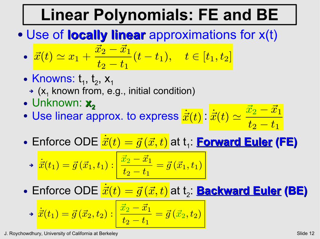
Linear Polynomials: FE and BE● Use of locally linearlocally linear approximations for x(t)

●

● Knowns: t1, t2, x1➔ (x1 known from, e.g., initial condition)

● Unknown: xx22● Use linear approx. to express :

● Enforce ODE at t1: Forward EulerForward Euler (FE) (FE)

➔

● Enforce ODE at t2: Backward EulerBackward Euler (BE) (BE)

➔

~x(t) ' x1 +~x2 ¡ ~x1t2 ¡ t1

(t¡ t1); t 2 [t1; t2]

_~x(t) _~x(t) ' ~x2 ¡ ~x1t2 ¡ t1

_~x(t) = ~g (~x; t)

_~x(t1) = ~g (~x1; t1) :~x2 ¡ ~x1t2 ¡ t1

= ~g (~x1; t1)

_~x(t) = ~g (~x; t)

_~x(t1) = ~g (~x2; t2) :~x2 ¡ ~x1t2 ¡ t1

= ~g (~x2; t2)

J. Roychowdhury, University of California at Berkeley Slide 13

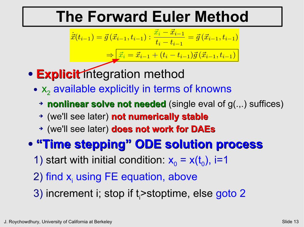
The Forward Euler Method

● ExplicitExplicit integration method● x2 available explicitly in terms of knowns

➔ nonlinear solve not needednonlinear solve not needed (single eval of g(.,.) suffices)➔ (we'll see later) not numerically stablenot numerically stable➔ (we'll see later) does not work for DAEsdoes not work for DAEs

● ““Time stepping” ODE solution processTime stepping” ODE solution process1) start with initial condition: x0 = x(t0), i=1

2) find xi using FE equation, above

3) increment i; stop if ti>stoptime, else goto 2

_~x(ti¡1) = ~g (~xi¡1; ti¡1) :~xi ¡ ~xi¡1ti ¡ ti¡1

= ~g (~xi¡1; ti¡1)

) ~xi = ~xi¡1 + (ti ¡ ti¡1)~g (~xi¡1; ti¡1)

J. Roychowdhury, University of California at Berkeley Slide 14

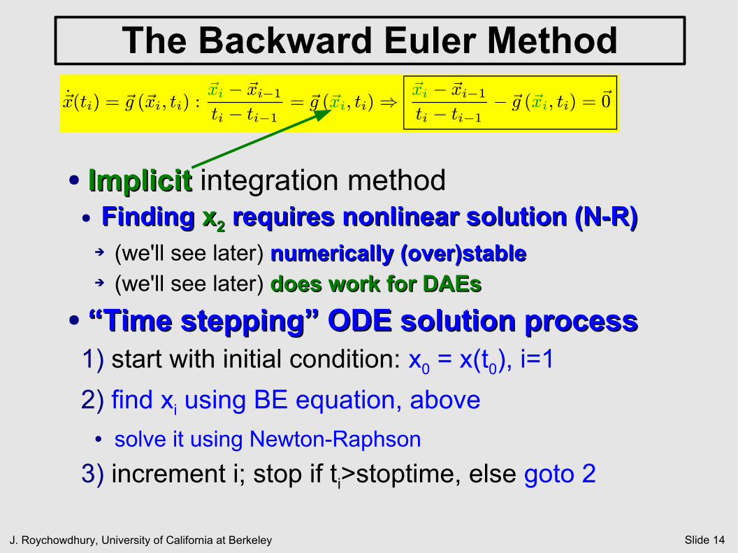
The Backward Euler Method

● ImplicitImplicit integration method● Finding Finding xx22 requires nonlinear solution (N-R)requires nonlinear solution (N-R)

➔ (we'll see later) numerically (over)stablenumerically (over)stable➔ (we'll see later) does work for DAEsdoes work for DAEs

● ““Time stepping” ODE solution processTime stepping” ODE solution process1) start with initial condition: x0 = x(t0), i=1

2) find xi using BE equation, above● solve it using Newton-Raphson

3) increment i; stop if ti>stoptime, else goto 2

_~x(ti) = ~g (~xi; ti) :~xi ¡ ~xi¡1ti ¡ ti¡1

= ~g (~xi; ti))~xi ¡ ~xi¡1ti ¡ ti¡1

¡ ~g (~xi; ti) = ~0

J. Roychowdhury, University of California at Berkeley Slide 15

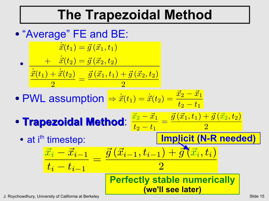
The Trapezoidal Method● “Average” FE and BE:

●

● PWL assumption

● Trapezoidal MethodTrapezoidal Method:

● at ith timestep:

_~x(t1) = ~g (~x1; t1)

+ _~x(t2) = ~g (~x2; t2)

_~x(t1) + _~x(t2)

2=~g (~x1; t1) + ~g (~x2; t2)

2

) _~x(t1) = _~x(t2) =~x2 ¡ ~x1t2 ¡ t1

~x2 ¡ ~x1t2 ¡ t1

=~g (~x1; t1) + ~g (~x2; t2)

2

~xi ¡ ~xi¡1ti ¡ ti¡1

=~g (~xi¡1; ti¡1) + ~g (~xi; ti)

2

Implicit (N-R needed)

Perfectly stable numerically(we'll see later)

J. Roychowdhury, University of California at Berkeley Slide 16

FE, BE, TRAP: Pictorial Summary

● Difference: where/how ODE is “enforced”

J. Roychowdhury, University of California at Berkeley Slide 17

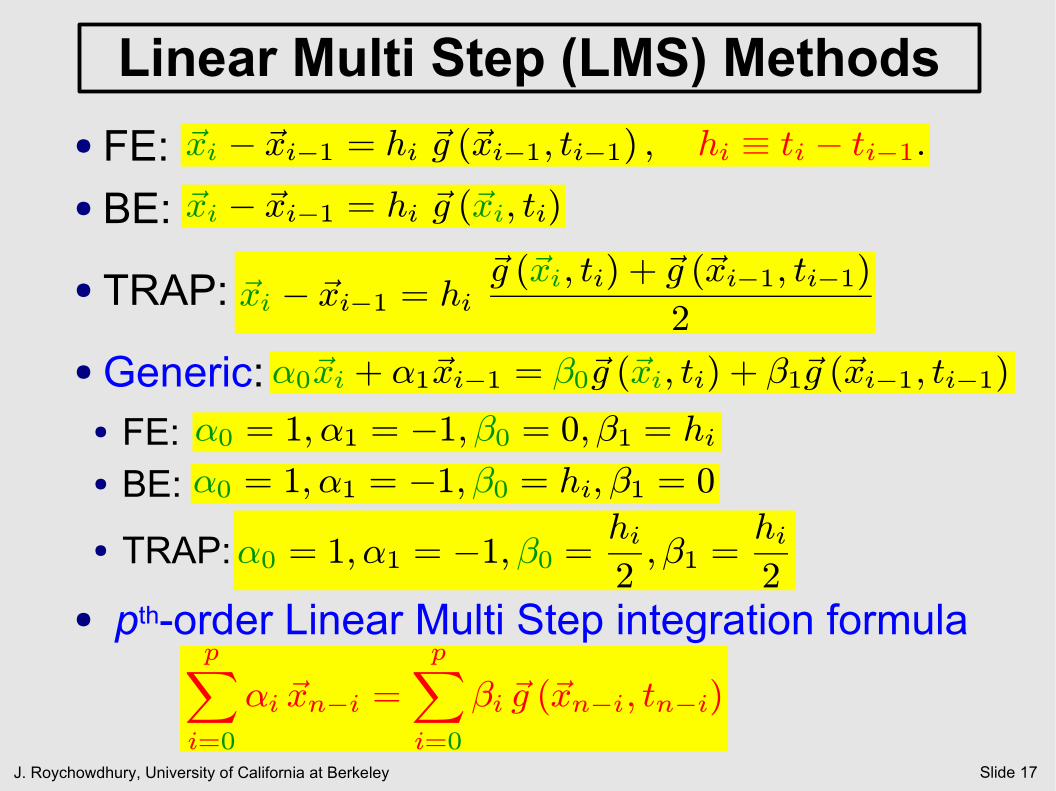
Linear Multi Step (LMS) Methods

● FE: ● BE:

● TRAP:

● Generic:● FE:● BE:

● TRAP:

● pth-order Linear Multi Step integration formula

~xi ¡ ~xi¡1 = hi ~g (~xi¡1; ti¡1) ; hi ´ ti ¡ ti¡1:~xi ¡ ~xi¡1 = hi ~g (~xi; ti)

~xi ¡ ~xi¡1 = hi~g (~xi; ti) + ~g (~xi¡1; ti¡1)

2

®0~xi + ®1~xi¡1 = ¯0~g (~xi; ti) + ¯1~g (~xi¡1; ti¡1)

®0 = 1; ®1 = ¡1; ¯0 = 0; ¯1 = hi®0 = 1; ®1 = ¡1; ¯0 = hi; ¯1 = 0

®0 = 1; ®1 = ¡1; ¯0 =hi2; ¯1 =

hi2

pX

i=0

®i ~xn¡i =pX

i=0

¯i ~g (~xn¡i; tn¡i)

J. Roychowdhury, University of California at Berkeley Slide 18

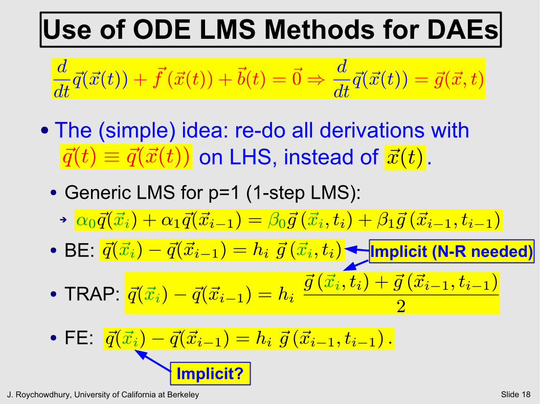
Use of ODE LMS Methods for DAEs

● The (simple) idea: re-do all derivations with on LHS, instead of .

● Generic LMS for p=1 (1-step LMS): ➔

● BE:

● TRAP:

● FE:

d

dt~q(~x(t)) + ~f (~x(t)) +~b(t) = ~0) d

dt~q(~x(t)) = ~g(~x; t)

~q(t) ´ ~q(~x(t)) ~x(t)

®0~q(~xi) + ®1~q(~xi¡1) = ¯0~g (~xi; ti) + ¯1~g (~xi¡1; ti¡1)

~q(~xi)¡ ~q(~xi¡1) = hi ~g (~xi; ti)

~q(~xi)¡ ~q(~xi¡1) = hi~g (~xi; ti) + ~g (~xi¡1; ti¡1)

2

~q(~xi)¡ ~q(~xi¡1) = hi ~g (~xi¡1; ti¡1) :

Implicit (N-R needed)

Implicit?

J. Roychowdhury, University of California at Berkeley Slide 19

Stability of LMS Methods

● Test ODE: ● exact solution:

➔ solution decays if

● What do FE/BE/TRAP produce?

_x(t) = ¸x(t); x(0) = x0:

x(t) = x0et :

¸ < 0:

FE is qualitatitivelywrong

J. Roychowdhury, University of California at Berkeley Slide 20

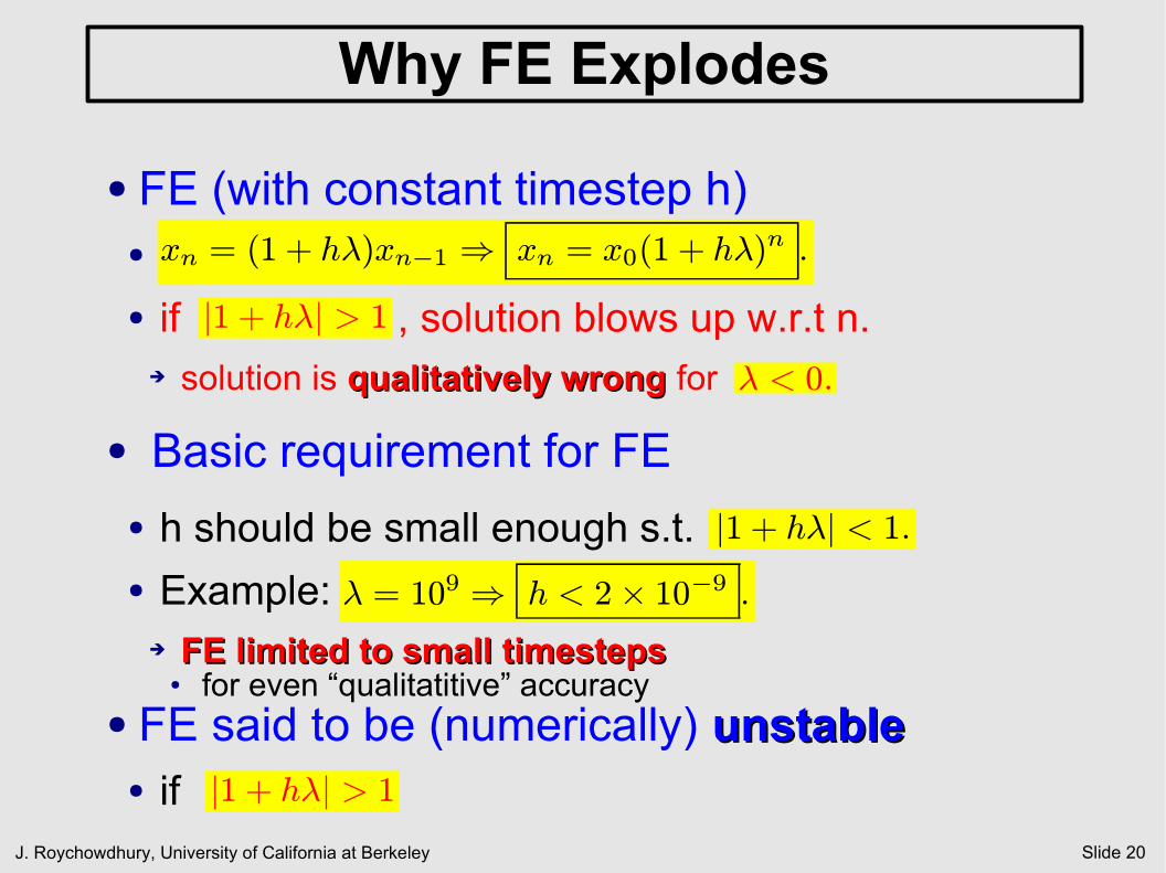
Why FE Explodes

● FE (with constant timestep h)● ● if , solution blows up w.r.t n.

➔ solution is qualitatively wrongqualitatively wrong for

● Basic requirement for FE

● h should be small enough s.t. ● Example:

➔ FE limited to small timestepsFE limited to small timesteps● for even “qualitatitive” accuracy

● FE said to be (numerically) unstableunstable● if

xn = (1 + h¸)xn¡1 ) xn = x0(1 + h¸)n :

j1 + h¸j > 1¸ < 0:

j1 + h¸j < 1:¸ = 109 ) h < 2£ 10¡9 :

j1 + h¸j > 1

J. Roychowdhury, University of California at Berkeley Slide 21

FE: Stability Picture for Complex ● In general: eigenvalues can be complex

● stability condition : circlecircle in h plane j1 + h¸j < 1

Region ofstability

J. Roychowdhury, University of California at Berkeley Slide 22

Stability of BE● BE with constant timestep h

●

● solution will die down if

➔ i.e., all of left half plane.● but also

➔ much of right half plane➔ BE is overstableBE is overstable

● OK only within circleOK only within circle

● ApplicationsApplications● more important more important● much better than FEmuch better than FE

xn(1 ¡ h¸) = xn¡1 ) xn = x01

(1¡ h¸)n :

j1¡ h¸j > 1:

J. Roychowdhury, University of California at Berkeley Slide 23

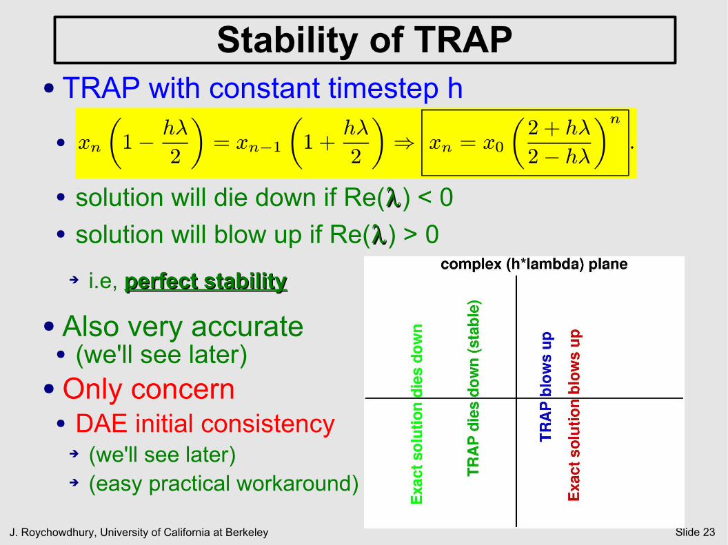
Stability of TRAP● TRAP with constant timestep h

●

● solution will die down if Re() < 0● solution will blow up if Re() > 0

➔ i.e, perfect stabilityperfect stability

● Also very accurate● (we'll see later)

● Only concern● DAE initial consistency

➔ (we'll see later)➔ (easy practical workaround)

xn

µ1¡ h¸

2

¶= xn¡1

µ1 +

h¸

2

¶) xn = x0

µ2 + h¸

2¡ h¸

¶n:

J. Roychowdhury, University of California at Berkeley Slide 24

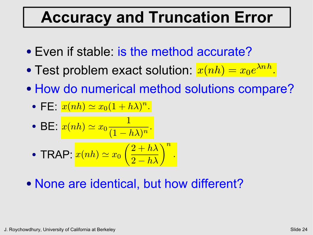
Accuracy and Truncation Error

● Even if stable: is the method accurate?● Test problem exact solution:● How do numerical method solutions compare?

● FE:

● BE:

● TRAP:

● None are identical, but how different?

x(nh) = x0e¸nh:

x(nh) ' x0(1 + h¸)n:

x(nh) ' x01

(1¡ h¸)n :

x(nh) ' x0µ2 + h¸

2¡ h¸

¶n:

J. Roychowdhury, University of California at Berkeley Slide 25

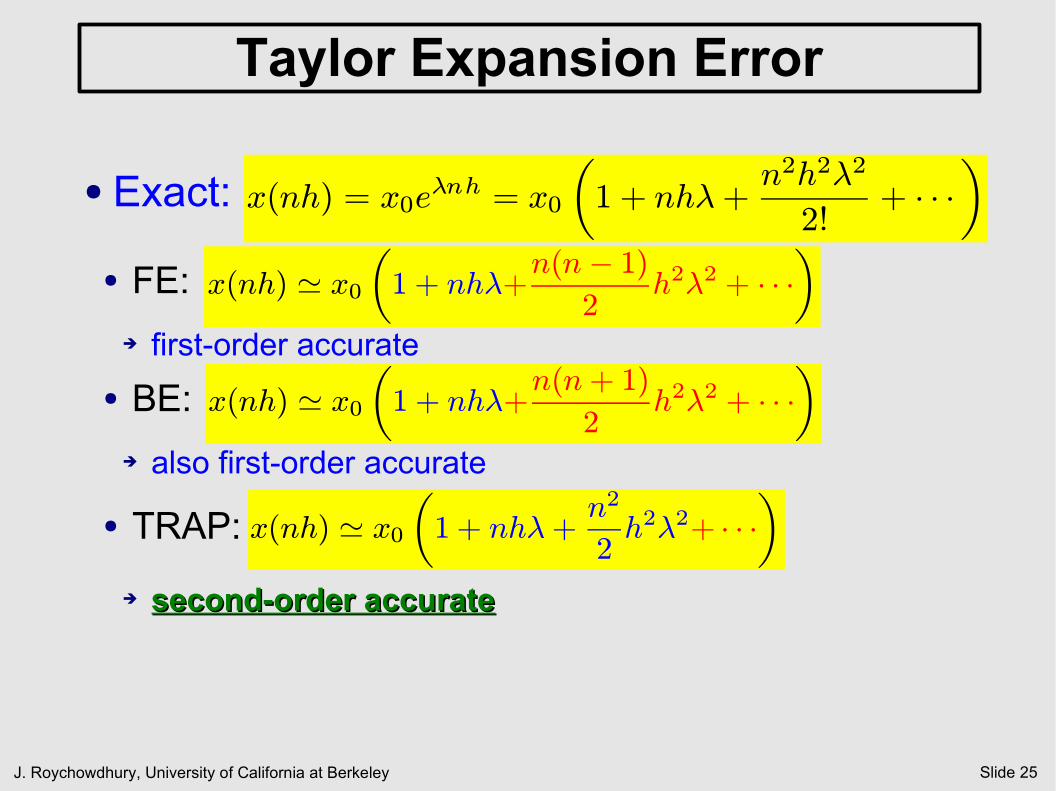
Taylor Expansion Error

● Exact:

● FE:

➔ first-order accurate

● BE:

➔ also first-order accurate

● TRAP:

➔ second-order accuratesecond-order accurate

x(nh) = x0e¸nh = x0

µ1 + nh¸+

n2h2¸2

2!+ ¢ ¢ ¢

¶

x(nh) ' x0µ1 + nh¸+

n(n¡ 1)2

h2¸2 + ¢ ¢ ¢¶

x(nh) ' x0µ1 + nh¸+

n(n+ 1)

2h2¸2 + ¢ ¢ ¢

¶

x(nh) ' x0µ1 + nh¸+

n2

2h2¸2+ ¢ ¢ ¢

¶

J. Roychowdhury, University of California at Berkeley Slide 26

Transient: Timestep Control● Choosing the next timestep dynamically● LTE based control

● apply LTE formulae to estimate error➔ change timestep to meet some specified error

● error specification: like reltol-abstol (reltol=percentage)➔ make sure these are looser than NR tolerances!

● element-by-element vs vector norm based➔ 2-norm vs max norm; DAE issues

● (change integration method based on timestep)● NR convergence based control

● cut timestep if NR does not converge➔ also: increase maxiter

● increase timestep if NR converges “too easily”➔ also: decrease maxiter

J. Roychowdhury, University of California at Berkeley Slide 27

ODE/DAE Packages Out There

● MATLAB has various ODE/DAE integrators● ode23, ode45, ...; ode23t, ode15s, ...

● DASSL/DASPK: general purpose DAE packages

● Linda Petzold, UCSB● Fortran● some tweaking helpful for circuit applications

● Easy (and often worthwhile) to roll your own● tweaking, special heuristics, debugging, ...

J. Roychowdhury, University of California at Berkeley Slide 28

Transient: Other Important Issues● What integration method to use?

● stability?● nonlinear solution required? (implicit vs explicit)● accuracy loss due to discretization?

➔ Local Truncation Error (LTE)➔ higher order methods (more than 1 previous timepoint)

● Vast body of work on ODE integration● linear multi-step methods (LMS), Runge-Kutta,

symmetric, symplectic, “energy-conserving”, etc.● Stiff differential equations

● different variables have very different time constants

➔ stiffly stable methods allow you to take larger time steps● DAE issues

● initial condition consistency; stability; index; …● Dynamic timestep control, NR heuristics, ...

J. Roychowdhury, University of California at Berkeley Slide 29

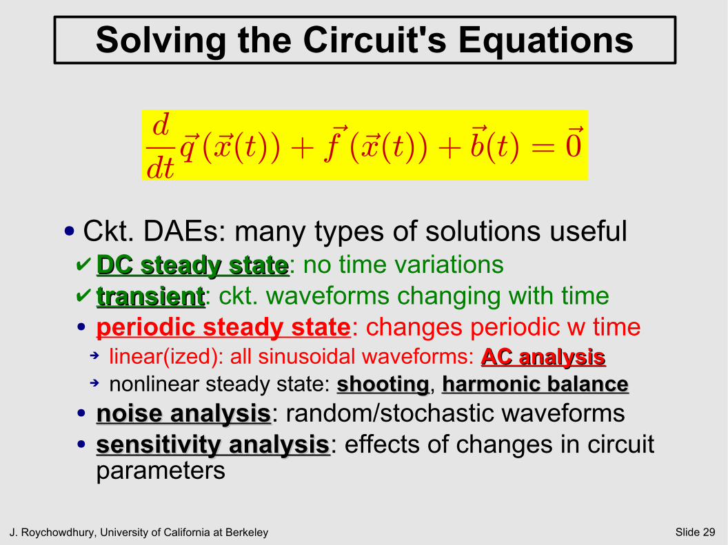
Solving the Circuit's Equations

● Ckt. DAEs: many types of solutions useful DC steady stateDC steady state: no time variations transienttransient: ckt. waveforms changing with time● periodic steady state: changes periodic w time

➔ linear(ized): all sinusoidal waveforms: AC analysisAC analysis➔ nonlinear steady state: shootingshooting, harmonic balanceharmonic balance

● noise analysisnoise analysis: random/stochastic waveforms● sensitivity analysissensitivity analysis: effects of changes in circuit

parameters

d

dt~q (~x(t)) + ~f (~x(t)) +~b(t) = ~0

J. Roychowdhury, University of California at Berkeley Slide 30

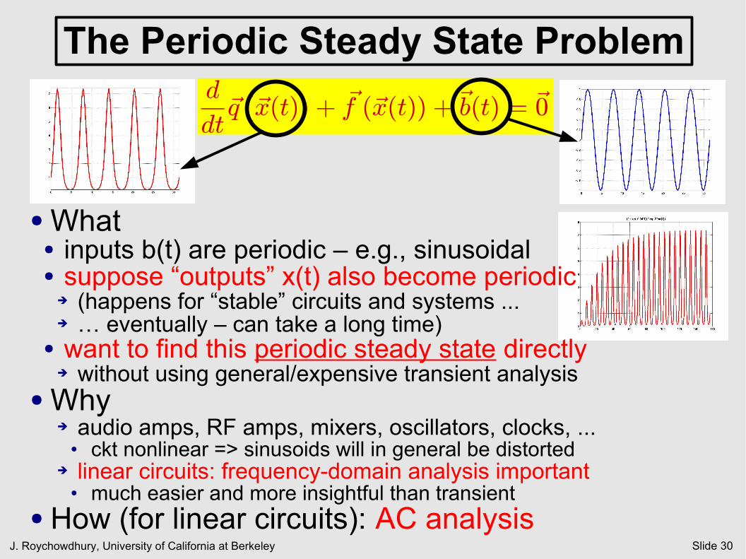
The Periodic Steady State Problem

● What● inputs b(t) are periodic – e.g., sinusoidal● suppose “outputs” x(t) also become periodic

➔ (happens for “stable” circuits and systems ...➔ … eventually – can take a long time)

● want to find this periodic steady state directly➔ without using general/expensive transient analysis

● Why➔ audio amps, RF amps, mixers, oscillators, clocks, ...

● ckt nonlinear => sinusoids will in general be distorted➔ linear circuits: frequency-domain analysis important

● much easier and more insightful than transient● How (for linear circuits): AC analysis

d

dt~q (~x(t)) + ~f (~x(t)) +~b(t) = ~0