Embed Size (px)
Citation preview
1
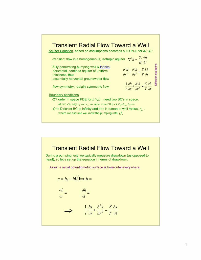
Aquifer Equation, based on assumptions becomes a 1D PDE for h(r,t) :
-transient flow in a homogeneous, isotropic aquifer
-fully penetrating pumping well & infinite,
horizontal, confined aquifer of uniform
thickness, thus
essentially horizontal groundwater flow
-flow symmetry: radially symmetric flow
Boundary conditions
-2nd order in space PDE for h(r,t) , need two BC’s in space,
at two r’s, say r1 and r2; in general we’ll pick r1=rw, r2=!
-One Dirichlet BC at infinity and one Neuman at well radius, rw ,
where we assume we know the pumping rate, Qw
t
h
K
Sh
s
!
!="
2
Diffu
sio
n e
quations
t
h
T
S
r
h
r
h
r !
!=
!
!+
!
!2
21
Transient Radial Flow Toward a Well
t
h
T
S
y
h
x
h
!
!=
!
!+
!
!2
2
2
2
During a pumping test, we typically measure drawdown (as opposed to
head), so let’s set up the equation in terms of drawdown.
Assume initial potentiometric surface is horizontal everywhere.
( ) shhthhs !="!=00
t
s
t
h
r
s
r
h
!
!"=
!
!
!
!"=
!
! ,
t
s
T
S
r
s
r
s
r !
!=
!
!+
!
!2
21
Transient Radial Flow Toward a Well
!
"

2
To solve, we need boundary conditions and initial conditions
I.C.: drawdown is zero, or head is uniform initially. s = 0 @ t ! 0
B.C.s : 2nd order equation, we need two BCs
Use r = 0, r = "
rbA !2=
Transient Flow Well Test Analysis
r
srT
r
sKbrQ
!
!=
!
!= 2 2 ""
r
sKA
r
hKAQr
!
!=
!
!"== ,0At
Use continuity at the pumping well, treated as a line sink (r = 0)
Transient Flow Well Test Analysis
r
srT
r
sKbrQ
!
!=
!
!= 2 2 ""
T
Q
r
sr
2!=
"
"
T
Q
r
sr
r !2lim
0
"#$
%&'
(
)
)"
(requires constant Q)
s # 0 as r # " (for all t)
3
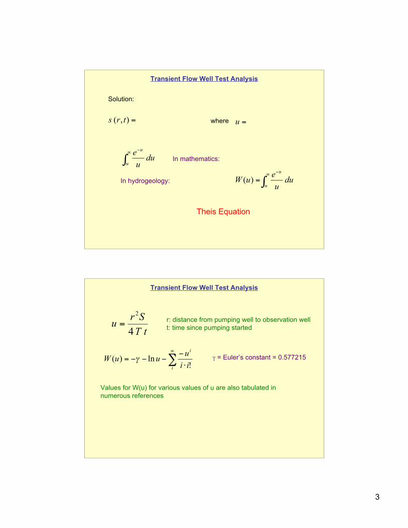
Transient Flow Well Test Analysis
Solution:
duu
e
T
Qtrs
u
u
4
),( !"
#
=$
where
tT
Sru
4
2
=
duu
e
u
u
!"
#
In mathematics: “The exponential integral”
)( 4
uWT
Qs
!=
In hydrogeology: “The well function” duu
euW
u
u
)( !"
#
=
Theis Equation
Transient Flow Well Test Analysis
tT
Sru
4
2
=r: distance from pumping well to observation well
t: time since pumping started
!"
#
$$$$=
i
i
ii
uuuW
!ln)( % $ = Euler’s constant = 0.577215
Values for W(u) for various values of u are also tabulated in
numerous references

4
Transient Flow Well Test Analysis
)( 4
uWT
Qs
!=
tT
Sru
4
2
=
Our goal in aquifer testing is to find T and S; solving the drawdown
equation shown above for T is problematic—T appears twice.
One way to solve for T is to compare a plot of s versus t to a
“normal” graphic solution (when plotting data from numerous
observation wells, we can typically normalize s by plotting it
as a function of t/r2 instead of t)
Transient Flow Well Test Analysis
“Type curve method” for solving the Theis Equation
•Plot s versus t (or s versus t/r2) on log-log paper
•On another sheet of the same paper, plot W(u) versus 1/u
Why 1/u? Our plot has t in the numerator, but in the
equation defining u, t appears in the denominator
•Match data (keep graph axes parallel)
•Pick “match point”—easiest to pick a match point with
simple numbers—the match point does not have to
fall on the curve.
•Solve equation
tT
Sru
4
2
=

5
Transient Flow Well Test Analysis
(Schwartz and Zhang, 2003)
Transient Flow Well Test Analysis
Q = 500 m3/d
r = 300 m
(Schwartz and Zhang, 2003)

6
m 78.0s min; 22 t;1.01
;1)( o ====o
o
o
uuW
Transient Flow Well Test Analysis
d
m 151
m) 0.78( 4
d
m500
)( 4
2
3
o
=!==""
ouWs
QT
( )
( )2
2
m 300
1.0min 1440
1dmin 22
d
m514
22 4
4!"
#$%
&!!"
#$$%
&
=!"
#$%
&==
o
o
oo
r
tuT
r
utTS
= 3.46 x 10⁻⁶
But S is hard to measure—typically should only
be reported to one significant digit id est 3 x 10⁻⁶
Transient Flow Well Test Analysis
Assumptions:•Homogeneous, isotropic aquifer (we used a simplified form of the
continuity equation instead of including the tensor for K)
•Constant water properties
•Infinite aquifer (used to develop boundary condition)
•Aquifer is confined; confining units are impermeable
•All flow is radial and horizontal
•Water is withdrawn instantaneously with decline in head
(not typically the case for leakage from confining units or
low k lenses)
•Well diameter is infinitesimal
(water can be stored in the well bore, leading to
‘delayed’ drawdown)
•Constant discharge from well

7
Head of NMT Hydrology Program
• C.E. Jacob (1965-1970)• Hantush’s mentor, well hydraulics,
theory of leaky aquifers
• 3 faculty, including Frank Titus and
William Brutsaert
• merged with Geology and Geophysics
to form Geosciences Department
• died of heart attack in 1970; Hantush
returned briefly
Simplified approach to transient analysis: The Jacob Approximation
A simplifying assumption that makes solving the Theis equation easier
C. E. Jacob (1940) “Jacob approximation” “Jacob-Cooper equation”
“Cooper-Jacob method” “Cooper-Jacob straight-line method”
!"
#
$$$$=
i
i
ii
uuuW
!ln)( %
...!44!33!22
ln577216.0)(432
+!
"!
+!
"+""=uuu
uuuW
Transient Radial Flow Toward a Well
8
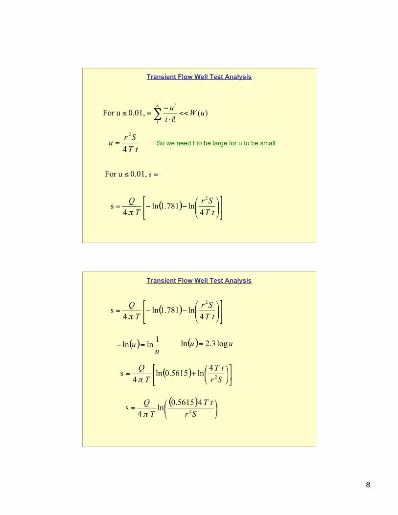
Transient Flow Well Test Analysis
)(!
0.01, u For uWii
u
i
i
<<!
"=# $
%
tT
Sru
4
2
= So we need t to be large for u to be small
( )uT
Qln577.0
4s 0.01, u For !!="
#
( ) !"
#$%
&''(
)**+
,--=
tT
Sr
T
Q
4ln781.1ln
4s
2
.
Transient Flow Well Test Analysis
( ) !"
#$%
&''(
)**+
,--=
tT
Sr
T
Q
4ln781.1ln
4s
2
.
( )u
u1
lnln =! ( ) uu log 3.2ln =
( ) !"
#$%
&'(
)*+
,+=
Sr
tT
T
Q2
4ln5615.0ln
4s
-
( )!"
#$%
&=
Sr
tT
T
Q2
4 5615.0ln
4s
'

9
Transient Flow Well Test Analysis
( )!"
#$%
&=
Sr
tT
T
Q2
4 5615.0ln
4s
'
( ) uu log 3.2ln =
Jacob-Cooper simplification
Transient Flow Well Test Analysis
Suppose we measure drawdown at two times: t1, t2
!"
#$%
&'()
*+,
-'+(
)
*+,
-='
122212ln
.252lnln
.252ln
4 t
Sr
Tt
Sr
T
T
Qss
.
[ ]1212
lnln 4
ttT
Qss !=!
"
1
2
12ln
4
t
t
T
Qss
!="
10
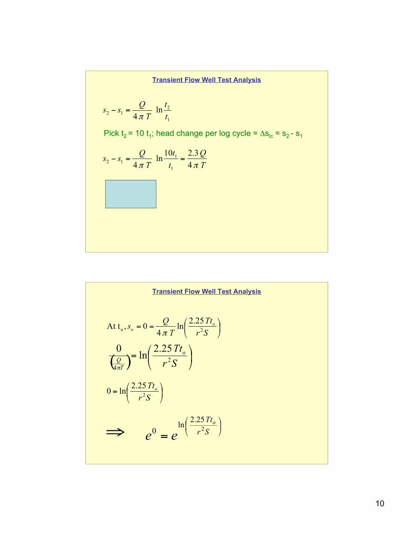
Transient Flow Well Test Analysis
1
2
12ln
4
t
t
T
Qss
!="
Pick t2 = 10 t1; head change per log cycle = %slc = s2 - s1
T
Q
t
t
T
Qss
4
3.210ln
4
1
1
12
!!=="
Transient Flow Well Test Analysis
.252
ln 4
0,At t 2o !
"
#$%
&==
Sr
Tt
T
Qs oo
'
.252
ln 0 2
!"
#$%
&=
Sr
Tto
2
.252ln
0!"
#$%
&
= Sr
Tto
ee
( )
.252ln
0
2
4
!"
#$%
&=
Sr
Tto
T
Q
'
!
"

11
Transient Flow Well Test Analysis
2
.252ln
0!"
#$%
&
= Sr
Tto
ee
Sr
Tto
2
.2521 =
Transient Flow Well Test Analysis
(Schwartz and Zhang, 2003)
Q = 500 m3/d
Semi-log plot (drawdown versus log time)

12
Transient Flow Well Test Analysis
lcs 4
3.2
!=
"
QT
( )( ) d
md
m2
3
51m .811 4
500 3.2==
!T
2
.252
r
TtS
o=
!
S =2.25 51
m2
d( ) 3.4min 1 d
1440min( )
300 m( )2
= 3 x 10"6
Transient Flow Well Test Analysis
tT
Sru
4
2
=
Remember that the Jacob-Cooper method is predicated on
the value of u being less than about 0.01!
( ) ( )( )( )
02.0min100 51 4
10 x 3m 300
min1440
d 1
d
m
62
2==
!
u
According to your textbook, 0.02 is “close” to 0.01, and it is
the maximum value of u over our log cycle of data, so the
Jacob-Cooper method is acceptable.

13
Transient Flow Well Test Analysis
Instead of looking at drawdown in one well with time, we can also look
at drawdown measured at the same time in two or more wells:
“Distance-drawdown method”
s1 (r1)
s2 (r2)Measured at the same time t
(Schwartz and Zhang, 2003)
r1
r2
Transient Flow Well Test Analysis
!"
#$%
&=
Sr
tT
T
Q2
.252ln
4s
'2
2ln
.252ln
.252ln
i
i
rS
tT
Sr
tT!"#
$%&
'=""
#
$%%&
'
!"
#$%
&+'(
)*+
,--'
(
)*+
,=- 2
2
2
121ln
.252lnln
.252ln
4 r
S
tTr
S
tT
T
Qss
.
!
s1" s
2=
Q
4 # T"ln r
1
2 + ln r2
2[ ]
1
2
21ln
4
2
r
r
T
Qss
!="

14
1
2
21ln
4
2
r
r
T
Qss
!="
Transient Flow Well Test Analysis
T
r
rQ
ss 2
ln
1
2
21
!
""#
$%%&
'
=(
s
r
rQ
T!
""#
$%%&
'
= 2
ln
1
2
(
Distance-drawdown formula
Transient Flow Well Test Analysis
Distance-drawdown formula
Remember that there are two formulae for applying the
Jacob-Cooper method—time-drawdown and distance-drawdown
2
.252
r
TtS
o=
To calculate S, we use a formula similar to that used in the
time-drawdown formula.
We used to because it told us the time at which drawdown was zero;
for a distance-drawdown formula, we want to know the distance at
which s = 0 (we’ll call it ro)—the rest of the derivation is the same as
for the distance-drawdown method, so we’ll jump right to the
formula:
2
.252
or
TtS =

15
Transient Flow Well Test Analysis
(Schwartz and Zhang, 2003)
Q = 220 gpm
= 29.41 ft3/min
= 42,350 ft3/d
Drawdowns
measured at
t = 220 min
Transient Flow Well Test Analysis
lcs 4
3.2
!=
"
QT
( )( ) d
ftd
ft2
3
987ft 5.71 4
42350 3.2==
!T
2
.252
or
TtS =
tT
Sru
4
2
=
!
S =2.25 987
ft2
d( ) 220min( )
1900 ft( )2
= 9 x 10"5
!
u =1900 ft( )
2
9 x 10"5( )
4 987ft2
d( ) 220min( ) 1 d1440min( )[ ]
= 0.54

16
Transient Flow Well Test Analysis
s
r
rQ
T!
""#
$%%&
'
= 2
ln
1
2
( lch
r
rQ
T!
""#
$%%&
'
= 2
10ln
1
1
(
Distance-drawdown formula Thiem equation
Transient Flow Well Test Analysis
s
r
rQ
T!
""#
$%%&
'
= 2
ln
1
2
( lch
r
rQ
T!
""#
$%%&
'
= 2
10ln
1
1
(
Distance-drawdown formula Thiem equation
Formulation of the DDF is identical to that of the Thiem equation
This means that when Jacob’s approximation applies, the difference in
drawdown between any two points stabilizes—the potentiometric surface
is being drawn down uniformly with time

17
Transient Flow Well Test Analysis
Why doesn’t this apply in early time? Stability is achieved when the
slope of the potentiometric surface has the correct gradient to supply
Q to the well
We are constantly lowering the potentiometric surface—we must do
this to release water from storage. In early time, water is only released
from storage near the well, but as time gets large, water is supplied
from a larger area.
As the volume of aquifer supplying Q increases, less
change in head is needed to yield the same amount of
water, so the cone of depression increases at a
decreasing rate.

18
How do cones of depression vary from “normal” with changes in
aquifer properties, and how does this affect the drawdown hydrograph
of a monitoring well?
How might drawdown hydrographs vary from “normal” in situations
where our pumping test assumptions are not met?
Variations in drawdown
Cone of depression as a function of time
t = 1 min t = 10 min t = 120 min
(Hall, 1996)
T = 1000 gpd/ft;
S = 10-4;
Q = 300 gpm

19
Variations in drawdown
Variations with pumping rate
Q = 100 gpm Q = 300 gpm Q = 600 gpm
T = 1000 gpd/ft;
S = 10-4;
r = 100 ft
(Hall, 1996)
Variations in drawdown
Variations with storativity
S = 0.000001 S = 0.0001
S = 0.1 S = 10-4;
Q = 300 gpm;
r = 100 ft
S = 0.1
0.01
0.0010.0001
0.00001
(Hall, 1996)

20
Variations in drawdown
Variations with transmissivity
T = 500 gpd/ft T = 1, 000 gpd/ft T = 2,500 gpd/ft
S = 1000 gpd/ft;
Q = 300 gpm;
r = 100 ft
(Hall, 1996)
Sensitivity to T and S summarized
Low T: tight, deep cone; High T: wide, shallow cone
Freeze and Cherry (1979)
Low S:
High S:
Cone shape remains
similar, the cone
is just bigger
Low S, creates greater drawdown to produce a given volume of water; cone of
depression shape stays the same
Low T: hard to transmit water, most efficient production is from close in,
creates steeper gradients of s to produce water from close in.

![A MATLAB Simulink Library for Transient Flow Simulation of ... · lines to simulate the transient gas flow in pipelines [9]. Ke and Ti analyzed isothermal transient gas flow in the](https://img.pdfslide.us/doc/110x75/5e1febbc24ec09539e44d276/a-matlab-simulink-library-for-transient-flow-simulation-of-lines-to-simulate.jpg)