Numeri l wave modeling – Fundamentals, Model setup …shodhganga.inflibnet.ac.in/bitstream/10603/85324/8/08_chapter2.pdf · Numeri l wave modeling – Fundamentals, Model setup

31

Chapter 2

Numerical wave modeling – Fundamentals,

Model setup and Validation

2.1. Introduction

This chapter describes the background of numerical wave modeling, the state-of-

the-art wave model MIKE 21 SW, the required data and the validation of the model

results. In relation to wave modeling, different classes of wave models are also discussed.

Description of MIKE 21 SW model consists of the governing equations, input parameters,

calibration parameters, numerical schemes, as well as initial and boundary conditions.

Initially, the model simulations are performed for a nine month period in order to evaluate

the model performance. In the final section of this chapter, there is a detailed discussion

related to the evaluation of model results. An evaluation of the model performance is

necessary to test the reliability of model results. Moreover, the evaluation of model

results is carried out using in-situ and altimeter observations in both fair weather and

extreme weather conditions.

2.2. Numerical Wave Modeling

The history of the study of ocean wave dynamics goes back several centuries, but

reasonable understanding of the physical properties of ocean waves start to develop in the

early twentieth century. With progress in the understanding of the wave dynamics that

took place, considerable attention has been paid to the modeling of ocean waves. The

importance of wind-induced sea surface wave prediction was realized during World War

II, when there arose a need for the planning of amphibious operations. Thereafter, the first

operational wave prediction techniques were developed by Sverdrup and Munk (1947)

Numerical wave modeling- Fundamentals, Setup and Validation 32

around that period. These techniques were based on the significant wave height concept,

in a purely statistical sense, where the spectral character of the sea state was completely

neglected. Interest in the prediction of the sea state started to grow by the middle of the

last century especially after the concepts of wave spectrum and its evolution were

recognized. In the fifties, the wave energy spectrum was introduced by Pierson et al.,

(1955). This wave spectrum concept was based on the assumption that the sea surface

may be represented as a Fourier series of superimposed waves with different wave

lengths and with different directions. The wave energy spectrum would then represent the

mean wave energy at each of these Fourier modes. Several statistical parameters

describing the sea state like significant wave height, mean wave direction and mean wave

period etc can be extracted from the wave energy spectrum. The spectral-energy balance

equation, which describes the development of surface gravity wave field in space and

time, forms the mathematical foundation of all numerical wave prediction models. Wave

models solve this equation using different numerical methods.

The energy balance equation is given (WMO, 1998) as,

. 2.1

, where, E Ef, , x, t, is the two dimensional wave spectrum depending on frequency

,f, and direction of propagation , Cg is the deep-water group velocity .

The source term expressed on the right-hand side of the equation is given by,

! 2.2 The source-sink mechanisms describe the wind input term (Sin), the nonlinear wave-wave

interaction (Snl), dissipation or whitecapping (Sds). The wind input source term represents

the momentum transfer by the winds to the free surface of the ocean. The nonlinear wave-

wave interaction source function (Hasselmann, 1962) provides the ways for energy to be

transferred between frequency bands. It was the principal mechanism for the


downshifting of the peak frequency found in wind -generation wave growth field studies

(Hasselmann et al., 1973). Equation (2.1) is valid for deep water with no refraction and no

significant currents. Numerical solution of equation (2.1) is performed in two parts. The

time invariant portion of equation (2.1) is solved first for propagation of the energy in a

fixed grid system. The spectrum in a numerical wave model is comprised of individual

packets of energy described at each frequency and direction band. This solution assumes

linear superposition of energy. Thus each frequency and direction dependent component

can be treated independent of its neighbour. Once this step is performed, equation (2.1) is

solved for the temporal change of action that is effected by the source terms found in the

right hand side of the equation (Jensen, 2002). All wave models follow this procedure for

solving the energy balance equation.

2.2.1. First, second and third generation wave models

Wave models are classified in to first, second and third generation based on the

methods of handling nonlinear source term (WMO, 1998). First generation wave models

included only wave energy growth and dissipation. These models do not have an explicit

nonlinear wave-wave interaction function (Snl). Later, the importance of the wave-wave

interaction and its role in the distribution of energy in the spectrum has been studied.

Hence second generation wave models (e.g. Sea wave modeling project, SWAMP Group,

1985) include a parametric formulation of the nonlinear wave-wave interaction source

function. One critical assumption used in these models was that, the spectrum was to

conform to some pre-defined shape in frequency and direction, which means a reference

spectrum (e.g. JONSWAP spectral form, Hasselmann et al., 1973). Despite this

limitation, well tuned second generation wave model results compared well with the

increasingly available wave measurements. One significant outcome of the SWAMP

(SWAMP Group, 1985) was a rather large scale discrepancy in wave height estimates for


simple academic tests. It was concluded that the Snl parameterization was the primary

cause for the order of magnitude differences found. The wave modeling group under the

direction of Professor Klaus Hasselmann worked with the goals to overcome the

deficiencies in second generation models and to subsequently implement a consistent set

of source terms centered about a better formulation of Snl, (Hasselmann and Hasselmann,

1985; Hasselmann et, al., 1985). Third generation wave models became feasible with the

development of the Discrete Interaction Approximation (DIA) (Hasselmann et, al., 1985)

to the nonlinear interactions. The DIA is the center piece of the first 3G wave model

(WAM). Currently, there are many 3G spectral wave models (e.g. SWAN (Booij et al.,

1999), WAVE-WATCH (Tolman, 1991), MIKE 21 SW (DHI, 2005), which are being

used for wave prediction and hindcast studies.

2.2.2. The unstructured grid approach

Traditionally, third generation spectral wave models are solved using either an

Eulerian or a semi-Lagrangian approaches on rectangular structured meshes. Even with

computers of today, these models are computationally highly demanding. To resolve the

characteristic scales of the important physical phenomena in the coastal areas a fine mesh

is required. In the breaking zone, a resolution of the order of 10m is needed. A high

resolution is also needed to resolve the complex bottom topographies in shallow water

environments (Sørensen et al., 2004). The need of high resolution local models can be

achieved by using nesting technique, where a local model with a fine mesh is embedded

in a coarse mesh model. Usually a one way transfer of boundary condition from the

coarse mesh model to the fine mesh model is used. With the goal of reducing the

computational effort, it is desirable to introduce more flexible meshes as an alternative to

nested models. Control of node distribution allows for optimal usage of nodes and

adaptation of mesh resolution to the relevant physical scales. Flexible mesh can be


accomplished in a number of ways, e.g. multi block-curvilinear meshes, overlapping

meshes, local mesh refinement and unstructured meshes. Only a few examples of third

generation spectral model using flexible mesh have been presented. Recently, the

possibility of using curvilinear meshes has been implemented in the SWAN model (Booij

et al., 1999). Benoit et al. (1996) developed the model TOMAWAC based on semi-

Lagrangian approach, where an unstructured finite element technique was used for the

spatial discretization of the dependent variable. Practical applications may need new

numerical approaches such as unstructured grids.

MIKE 21 SW is a new generation spectral wind-wave model based on

unstructured meshes (Sörensen et al., 2004). Unstructured grid approaches are expected to

become more important for coastal applications. In coastal regions, the effect of tides,

surges and currents can be very important for accurate prediction of the wave conditions.

Due to the high degree of flexibility, unstructured meshes are very efficient to deal with

problems of different characteristic scales. For the maximum degree of flexibility, an

unstructured mesh approach has been chosen for this model. This feature of the model

makes its major application area as the design of offshore, coastal and port structures

where accurate assessment of wave loads is of utmost importance to the safe and

economic design of these structures. The source functions implemented in the MIKE 21

SW are based on state-of-the-art third generation formulations. MIKE 21 SW is used for

the assessment of wave climates in offshore and coastal areas in hindcast and forecast

mode. This is followed, in Section 2.3, by MIKE 21 SW model details and modeling

schemes.

2.3. MIKE 21 SW MODEL

MIKE 21 SW is the state-of-the-art third generation spectral wind-wave model

based on unstructured meshes developed by Danish Hydraulic Institute (DHI), Denmark.


The model simulates the growth, decay and transformation of wind generated waves and

swells in offshore and coastal areas. MIKE 21 SW is particularly applicable for

simultaneous wave prediction and analysis on regional and local scale. MIKE 21 SW

includes the following physical phenomena: (i) Wave growth by action of wind, (ii) Non-

linear wave-wave interaction, (iii) Dissipation due to white capping, (iv) Dissipation due

to bottom friction, (v) Dissipation due to depth induced wave breaking, (vi) Refraction

and shoaling due to depth variations, (vii) Wave-current interaction, (viii) Effect of time-

varying water depth.

MIKE 21 SW includes two different formulations namely, directional decoupled

parametric formulation and fully spectral formulation (DHI, 2005). The directional

decoupled parametric formulation is based on a parameterization of the wave action

conservation equation. The parameterization is made in the frequency domain by

introducing the zeroth and first moment of the wave action spectrum as dependent

variables Holthuijsen (1989). The fully spectral formulation is based on the wave action

conservation equation, as described in e.g. Komen et al. (1994) and Young (1999), where

the directional–frequency wave action spectrum is the dependent variable. The first

formulation is suitable for near shore and the second one is suitable for both near shore

and offshore spectral wave modeling. As the study area contains shallow water and

offshore regions, the fully spectral formulation in terms of the wave direction, θ, and the

relative angular frequency has been chosen for the present study.

2.4. Model Setup

2.4.1. Model domain and Bathymetry

In the present study, the model domain covers the Indian Ocean region, 60˚S-

25˚N; 40˚E-100˚ E (Fig.2.1).


Fig.2.1: Map of the study area showing flexible mesh grid

For the model runs, the spatial resolution has been chosen to be 0.25˚ in the coastal waters

and 1˚ for the rest of the region. This, however, does not mean that the resolution is

constant everywhere in this domain. MIKE21 SW model uses a flexible mesh bathymetry

for model runs. MIKE-21 has an in-built flexible mesh generator which generates flexible

bathymetry for model runs and the flexible mesh allows fine resolution near the coast.

The bathymetry is from GEBCO (details given in section 1.6 of Chapter 1).

2.4.2. Governing Equations

In the presence of dynamic depths and currents, the conserved quantity is wave

action (not energy) and the dynamics of gravity waves can be described by the

conservation equation for wave action density. In MIKE 21 SW model, the wind waves

are represented by the action density spectrum N(σ, θ). The independent phase parameters

have been chosen as the relative (intrinsic) angular frequency, σ=2πf, and the direction of


wave propagation, θ. The governing equation is the wave action balance equation formulated

in either Cartesian or spherical co-ordinates (Komen et. al., 1994 and Young, 1999). For

small scale applications, the basic conservation equations are usually formulated in Cartesian

co-ordinates, while spherical polar co-ordinates are used for large scale applications.

The conservation equation for wave action can be written as,

" . #$" S

& 2.3 Where N (($,&, , is the action density, t is the time, ($ =(x, y), #$ = ()*,)+,),,)-) is the

propagation velocity of a wave group in the four-dimensional phase space,($, & and θ and S is the source term for the energy balance equation. is the four dimensional

differential operator in the ($, &, θ-space.

2.4.3. Source functions

The source term S on the right hand side of Eq. (2.3) represents the superposition

of source functions describing various physical phenomena and is given by,

S /0/12 S34 S42 S56 S70/ S689: 2.4

Here Sin represents the generation of energy by wind, Snl is the wave energy transfer due

to non-linear wave-wave interaction, Sdis is the dissipation of energy due to white

capping, Sbot is the dissipation due to bottom friction and Ssurf is the dissipation of energy

due to depth-induced wave breaking. The default source functions Sin , Snl, and Sds in

MIKE 21 SW are similar to the source functions implemented in the WAM Cycle 4

model (Komen et al.,1994).

2.4.4. Wind input

Wind wave generation is the process by which the wind transfers energy in to the

water body for generating waves. The wind input, Sin, is based on Janssen’s (1989, 1991)


quasi-linear theory of wind-wave generation, where the momentum transfer from the

wind to the sea depends not only on the wind stress, but also on the sea state itself, and is

implemented as in WAM Cycle 4. In a series of studies by Janssen (1989) and Janssen

(1991), it is shown that the growth rate of the waves generated by wind also depends on

wave age. This is because of the dependence of the air drag on the sea state. The input

source term, Sin is given by,

<, = <, 2.5

, where γ is the growth rate. For a given wind speed and direction, the growth rate of

waves of a given frequency and direction depends on the friction velocity, ? *, and sea

roughness z0 In principle, if the sea roughness is known or assumed (e.g. the Charnock

parameter, @AB C@D/? FG, may be assumed) ,the wind friction speed can be estimated

using the logarithmic wind profile. Thus, the growth rate of waves due to wind input can

be calculated. Assuming a dimensionless sea roughness (@AB C@D/? FG) of 0.0144, this

formulation was shown in Komen et. al,(1994) to fit the observations compiled by Plant

(1982).

Two different formulations of air-sea interaction have been implemented in this

model. A “coupled” formulation means the momentum transfer from the wind to the

waves or drag depends not only on the wind but also on the waves according to the

formulation in Komen et al. (1994). An “uncoupled” formulation means the momentum

transfer from the wind to the waves solely depends on the wind speed, and consists of a

sea state independent roughness description. The default drag law is taken from Smith

and Banke (1975). In the present study a coupled formulation of air-sea interaction has

been used. A detailed description of wind fields used for driving the model in the present

study has been given in section 1.6 of Chapter one.


2.4.5. Nonlinear Interactions

The nonlinear energy transfer amongst the different wave components of a

directional frequency spectrum plays a crucial role for the temporal and spatial evolution

of a wave field. The nonlinear energy transfer, Snl, through the four wave interaction is

represented by the discrete interaction approximate (DIA) used for the present study. The

DIA was developed by S. Hasselmann et al. (1985). The quadruplet-wave interaction

controls (i) the shape-stabilization of the high-frequency part of the spectrum, (ii) the

downshift of energy to lower frequencies and (iii) frequency-dependent redistribution of

directional distribution functions. The discrete interaction approximate (DIA) is the

commonly used parameterization of Snl in third generation wave models. This DIA has

been found quite successful in describing the essential features of a developing wave

spectrum (Komen et al., 1994).

2.4.6. Calibration Factors

2.4.6.1. White capping source function

The source function describing the dissipation due to white capping is based on

the theory of Hasselmann (1974), tuned according to Janssen (1989). With the

introduction of Janssen’s (1989) description of wind input, it was realized that the

dissipation source function needs to be adjusted in order to obtain a proper balance

between the wind input and the dissipation at high frequencies. The source function is

given by,

!&, H !IJGKDG L1 H M IIJ M NI

IJOGP &J"&, 2.6

Where Cds (Cdis) and δ (DELTAdis) are 4.5 and 0.5 as suggested in Komen et al.,

(1994). IJ is the mean wave number and KD is the zeroth moment of the spectra.


2.4.6.2. Bottom friction source function

As wave propagates to the shallow water, the orbital velocities penetrate the water

depth and the source terms due to wave-bottom interaction processes become important.

The rate of dissipation, Sbot, due to bottom friction is based on linear theory (Weber, 1991)

and Johnson and Kofoed-Hansen, 2000). The friction coefficient is determined as the

product of a friction factor and the rms velocity at the bottom. The friction factor is

calculated using the expression by Jonsson (1966) and Jonsson and Carlson (1976). In the

expression by Jonsson the friction coefficient is determined as function of the bottom

roughness length scale, kN, and the orbital displacement at the bottom.

R&, HSI

TUVW2IW &, 2.7

Where Cf is the dissipation coefficient(=fw Ubm), which depends on the hydrodynamic and

sediment conditions. Here fw is the wave friction factor and Ubm is the maximum near-

bed particle velocity. MIKE 21 provides four dissipation formulations namely a constant

friction coefficient based on tests with regional versions of WAM model (Komen et al.,

1994), a constant friction factor proportional to rms wave orbital velocity at the bottom, a

constant geometric roughness size (Nikuradse roughness, kN, as suggested by (Weber et

al., 1991) in conjunction with friction factor expression of Jonsson and Carlsen(1976) and

a constant median sediment size D50. In the present study, the bottom friction is

considered according to Nikuradse roughness, kN. It is a calibration factor and the value

applied in the present study is 0.04 m.

2.4.6.3. Wave breaking source function

Depth-induced breaking occurs when waves propagate into very shallow areas,

and the wave height can no longer be supported by the water depth. The formulation of

wave breaking is based on the breaking model by Battjes and Janssen (1978). Eldeberky


and Battjes (1995) proposed a spectral version of the breaking model, where the spectral

shape was not influenced by the breaking .The source term due to depth-induced breaking

can be written as,

!YZS&, H [\R&J ]G8` &,

2.8 Here α (=1) is a calibration constant controlling the rate of dissipation and is a proportional

factor to the wave breaking source function. Qb is the fraction of breaking waves, σJ is the

mean relative frequency, Etot is the total wave energy and Hb γd is the maximum

wave height. Here, γ is the free breaking parameter (a wave height to depth ratio). Kaminsky

and Kraus (1993) found that γ values are in the range between 0.6 and 1.59 with an average

of 0.79. The value of the breaking parameter, γ, varies from 0.5 to 1.0. In the present study,

γ = 0.8 has been applied.

2.4.7. Numerical method

2.4.7.1. Space Discretization

The spatial discretization of conservation equation for wave action is performed

using an unstructured finite volume (FV) method (DHI, 2005). During the last decade, FV

methods have been successfully applied for modeling of non-linear transport problems

and compressive flow problems. In the geographical domain, an unstructured mesh is

used. The spatial domain is discretised by subdivision of the continuum into non-

overlapping elements. The elements can be of arbitrarily shaped polygons, however, in

this model only triangles are considered. The action density, N (xJ, σ, θ) is represented as a

piecewise constant over the elements and stored at the geometric centres (DHI, 2005). In

the frequency space, a logarithmic discretization is used,

σ1 =σmin , σl =fσσl-1, ∆σl = σl-1- σl+1, l=2, Nσ (2.9)


, where fσ is a given factor, σmin is the minimum discrete angular frequency and Nσ is the

number of discrete frequencies. In the directional space, an equidistant discretization is

used,

θm= (m-1)∆θ , ∆θm = 2π/Nθ , m = 1,Nθ (2.10) , where Nθ is the number of discrete directions. The action density is represented as a

piecewise constant over the discrete intervals, ∆σl and ∆θm, in the frequency and

directional space. In the present study, the minimum frequency is set to 0.055 Hz and the

number of frequencies is 25. For directional discretization, 360° rose has been considered.

The number of directions is set to 16.

Integrating the wave action conservation equation over area Ai of the ith element, the

frequency increment ∆σl and the directional increment ∆θm one obtains

∂∂t p∆θqp∆σrpstNdΩdσdθ H p∆θqp∆σrpstSσ

dΩdσdθ = p∆θqp∆σrpst. (FJ)dΩdσdθ (2.11)

Where Ω defines the differential element of the area Ai and FJ= (Fx,Fy,Fσ,Fθ) = νvN is the

convective flux. The volume integrals on the L.H.S of Eq. (2.11) are approximated by one

point quadrature rule. Using the divergence theorem, the volume integral on the right

hand side can be replaced by integral over the boundary of the volume in the xJ , σ, θ-

space and these integrals are evaluated using mid-point quadrature rule. Hence, Eq. (2.11)

can be written as,

∂N3,2,b∂t = H 1A3 xy(F4)z,2,b∆lz|

z~ H 1

∆σ2 (Fσ)3,2~/G,b H (Fσ)3,2~/G,b

H 1∆θb (Fθ)3,2,b~G H (Fθ)3,2,b~/G S3,2,b

σ2 (2.12)

Where NE is the total number of edges in the cell (NE=3 for triangles).

Numerical wave modeling- Fundamentals, Setup and Validation 44 F4z,2,b FN FNz,2,b, is the normal flux through the edge p in the geographical

space with length ∆lp. nJ =(nx , ny) is the outward pointing unit normal vector of the

boundary in the geographical space. Fσi,l+1/2,m and (Fθ)i,l,m+1/2 are the flux through the

face in the frequency and directional space, respectively.

The convective flux is derived using a first order upwinding scheme. The numerical

diffusion introduced using first order upwinding schemes can be significant, see e.g.

Tolman (1991, 1992). In small scale coastal applications and the application dominated

by the local wind, the accuracy obtained by using this scheme is considered to be

sufficient. However, for the case of swell propagation over long distances, higher-order

upwinding schemes may have to be applied.

2.4.7.2. Time integration

The time integration is based on a fractional step approach, where the propagation

step is solved using an explicit method. Firstly, a propagation step is performed

calculating an approximate solution at the new time level by solving Eq. (2.3) without

source terms. Secondly, a source term step is performed calculating the new solution from

the estimated solution taking into account only the effect of source terms.

The propagation step is carried out by an explicit Euler scheme. To overcome the severe

stability restriction, a multi sequence integration scheme is employed following the idea

by Vilsmeier and Hanel (1995). Here, the maximum time step is increased by locally

employing a sequence of integration steps, where the number of steps may vary from

element to element. Using the explicit Euler scheme, the time step is limited by the CFL

condition stated as

C9t,r,q C∆t∆x3

+ C∆t∆y3

+ Cσ ∆t∆σ2

+ Cθ ∆t∆θb

1 (2.13)


Here C9t,r,qis the Courant number and ∆x3 and ∆y3 are characteristic length scale in the x

and y-directions for the ith element. The maximum local courant number, Crmax,i ,is

determined for each element in the geographical space, and the maximum local time step

is given by

∆^*, ∆Z,

2.14 To ensure accuracy in time, the intermediate levels have to be synchronized. The time

step index g is determined as the minimum value for which

∆ < ∆^*, , < ~G~

, g=1,2,3 (2.15)

The local time step is then determined as ∆ = ∆ <, two neighbouring elements are not

allowed to have an index difference greater than one.

The calculation is performed using a group concept and the computational speed-up using

the multi sequence integration compared to the standard Euler method increases with

increasing number of groups. However, to get accurate result in time, the maximum

number of groups must be limited (DHI, 2005). In the present work maximum number of

levels is 32.

2.4.8. Initial conditions

The initial conditions are applied by calculating the spectra from empirical

formulations. In the present study, JONSWAP fetch growth expression has been applied

to calculate the spectra. The following values are used for various parameters: maximum

fetch length: 100 km; maximum peak frequency: 0.4 Hz; maximum Philip’s constant:

0.0081; shape parameter, σa: 0.07; shape parameter, σb: 0.09; peakness parameter, γ: 3.3.


2.4.9. Boundary Conditions

At the land boundaries in the geographical space, a fully absorbing boundary

condition is applied. The incoming flux components (the flux components for which the

propagation velocity is normal to the cell face is positive) are set to zero. No boundary

condition is needed for outgoing flux components. At an open boundary, the incoming

flux is needed. Hence, the energy spectrum has to be specified at an open boundary. In

the frequency space, the boundaries are fully absorbing. No boundary conditions are

needed in the directional space. In the present study, for wave simulations in the Indian

Ocean, all the boundaries were closed assuming that the influence of wave energy into the

Indian Ocean from the rest of the Oceans has negligible impact along the Indian coastal

regions. It means, no waves enter the model domain through this boundary and the

outgoing waves are fully absorbed.

2.4.10. Output parameters

At each mesh point and for each time step four types of output can be obtained

from MIKE 21 SW (i) Integral wave parameters (ii) Input parameters (iii) Model

parameters (iv) Spectral parameters.

The spectral parameters are wave energy and wave action. The directional-frequency

wave spectra at selected grid points and or areas as well as direction spectra and

frequency spectra can be obtained from MIKE 21 SW. We have used only the spectral

parameters and integral parameters for the present study.

The integral wave parameters can be computed for the total spectrum, for the wind sea

part of the spectrum and the swell part of the spectrum. The details of integral parameters

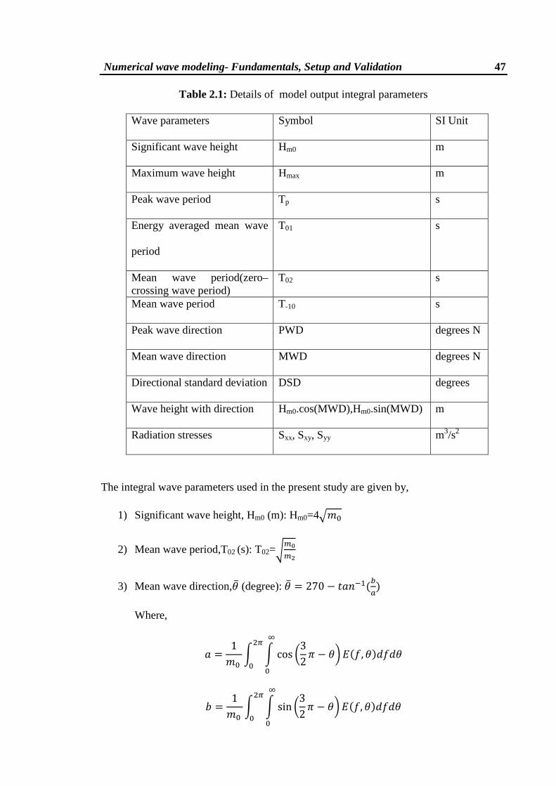
are given in Table 2.1.


Table 2.1: Details of model output integral parameters

Wave parameters Symbol SI Unit

Significant wave height Hm0 m

Maximum wave height Hmax m

Peak wave period Tp s

Energy averaged mean wave

period

T01 s

Mean wave period(zero–crossing wave period)

T02 s

Mean wave period T-10 s

Peak wave direction PWD degrees N

Mean wave direction MWD degrees N

Directional standard deviation DSD degrees

Wave height with direction Hm0.cos(MWD),Hm0.sin(MWD) m

Radiation stresses Sxx, Sxy, Syy m3/s2

The integral wave parameters used in the present study are given by,

1) Significant wave height, Hm0 (m): Hm0=4KD

2) Mean wave period,T02 (s): T02=^^

3) Mean wave direction,$ (degree): $ 270 H V~R

Where,

1KD cos N3

2 ` H O <, <

D

GD

1KD sin N3

2 ` H O <, <

D

GD


The distinction between wind-sea and swell can be calculated using either a constant

threshold frequency or a dynamic threshold frequency with an upper frequency limit. In

the present study a constant threshold frequency (=0.1 Hz) has been used for the

separation of wind-sea and swell as in the case of buoy data.

2.5. Model validation

Initially model run has been performed for a nine month period to evaluate the

model performance. The six hourly ECMWF blended wind analysis with a spatial

resolution of 0.25o has been used for this experiment (description of the wind field is

given in section 1.6 of Chapter 1). The model was initialized over a seven day period to

arrive at a stationary model output, and thereafter experiments were performed for the

period of January- September, 2006. Synoptic maps of wave parameters and time series

output for selected buoy location, both in shallow and off shore region, were generated

for the comparison. As mentioned earlier, wave data derived by moored buoys deployed

by the National Institute of Ocean Technology (NIOT) has been used for validating the

model results. Various statistical measures like Bias, Root Mean Square Error (RMSE),

Scatter Index (SI), and Correlation Coefficient (R) are used to assess the model

performance by comparing the model derived parameters against the corresponding

buoy/altimeter observations. The formulas for the statistical measures are,

Bias ~ ∑K¢ H £T 2.16

RMSE ~ ∑K¢ H £TG 2.17

SI RMSE/£TJJJJJ 2.18

§ ∑K¢ H K¢JJJJJ£T H £TJJJJJ∑K¢ H K¢JJJJJG£T H £TJJJJJG 2.19


Here obs denotes a particular wave parameter derived by the buoy/altimeter and mdl is

the corresponding model wave parameter. The over bar denotes the statistical average.

In many applications, only the heights and periods of the higher waves in a wave

train are of practical significance. For this reason, the average height and period of the

highest one-third of the waves are useful statistical measures. These averages have been

called "significant wave height" and “mean wave period". So the model performance has

been evaluated in terms of significant wave height (Hs), and mean wave period (Tm) in

both Arabian Sea (AS) and Bay of Bengal (BoB) by selecting 3 buoys from each basin

( locations of the buoys are shown in Fig.1.4). Among the three buoys, two buoys were

located at the offshore region (DS7, DS1 in Arabian Sea and DS5, OB8 in Bay of Bengal)

and one was located at the shallow water (SW4 in Arabian Sea and SW6 in Bay of

Bengal). The data were continuous for the considered time period for deep water buoys

DS7, OB8. In the case of DS5, DS1 data were missing. The missing period was two

months (Jun-Jul) for DS5 whereas DS1 provided only three months (Jun.-Aug.). The

shallow water buoys selected for the validation provided a discontinuous data series. SW4

buoy which is located in the Arabian Sea provided only four months data whereas the

SW6 buoy present in the Bay of Bengal could provide only one month data. Figures 2.2-

2.4 show the comparison of model derived significant wave height (Hs) and mean wave

period (Tm) with the corresponding buoy derived parameters. These figures show that

wave heights are quite low till March except high waves in a few isolated cases. Wave

height starts to increase from the end of April till the end of monsoon period. Very high

waves are observed by deep water buoys located in the Arabian Sea. In the case of DS1

buoy, wave height of the order of 7m is observed in July and the model derived wave

height exhibited very good agreement with observed data in the extreme waves also. The

wave height in the Bay of Bengal was low compared to the wave height in the Arabian


Sea, and the maximum height observed was around 4m. The model derived wave height

and mean wave period are in good agreement with the measured wave data in the shallow

water also. A very good agreement of buoy derived and model derived wave height can

be seen in for all the buoys in the low wave heights as well as in the extreme wave

heights. In the case of wave period a close match can be seen during most of the time but

in few cases mismatch are also noticeable.

Fig 2.2: Comparison of significant wave height and mean wave period for Arabian Sea

deep water Buoys (a) At DS7 Buoy location (b) At DS1 Buoy location


Fig 2.3: Comparison of significant wave height and mean wave period for Bay of Bengal

deep water Buoys (a) At DS5 Buoy location (b) At OB8 Buoy location


Fig.2.4: Comparison of significant wave height and mean wave period for shallow water

Buoys (a) At SW4 Buoy location in the Arabian Sea (b) At SW6 Buoy location in the

Bay of Bengal


For a detailed evaluation of model performance, statistical error analysis has been carried

out. Table 2.2 shows the error statistics of the comparison of all the buoys for both the

basins. The number of points, Bias, RMSE, Scatter Index (SI) and Correlation Coefficient

(R) of each buoy are given in Table 2.2.

Table 2.2: Model error statistics for the buoy comparison

Buoy No. of

Points

Parameters BIAS RMSE SI R

DS7

2075

Hs(m) 0.18 0.34 0.21 0.94

Tm(s) 0.49 0.92 0.15 0.76

DS1

814

Hs(m) -0.11 0.39 0.12 0.95

Tm(s) 0.46 0.68 0.10 0.84

OB8

2031

Hs(m) -0.08 0.24 0.17 0.92

Tm(s) -0.28 0.65 0.12 0.70

DS5

1737

Hs(m) 0.00 0.26 0.17 0.94

Tm(s) -0.30 0.91 0.15 0.69

SW4

1080

Hs(m) 0.09 0.16 0.24 0.70

Tm(s) 0.37 0.81 0.17 0.57

SW6

219

Hs(m) -0.32 0.39 0.28 0.69

Tm(s) -0.43 0.72 0.13 0.43

From Table 2.2, it can be seen that the simulated significant wave height values are in

good agreement with measured data with RMSE values ranging from 0.16-0.4 m. DS5

buoy shows a very good agreement in the case of wave height with practically no bias,

very low RMSE as well as SI and a good correlation. In the case of wave period a very

low scatter index was seen in all the buoys and the RMSE values were in the range of

0.65-0.92 s. High correlation is observed at four deep sea locations compared to that of


shallow water. The lower correlation at the coastal buoys may be due to the combined

effect of bottom topography and less accurate wind input. The error statistics clearly show

that model simulated waves are in good agreement with a low error and model is able to

simulate waves well, both in shallow and deep water regions. Model results also clearly

bring out wave patterns during the phases of pre-monsoon and monsoon. The validation

exercise establishes the reliability of the model in simulating the intra-annual variability

of wave characteristics in North Indian Ocean. Summarizing, it can be said that MIKE 21

SW is able to provide good quality simulation of wave characteristics at all the locations.

2.5.1. Evaluation of model performance during cyclonic condition

In the year 2006, during the period April 24-April 29, a very severe cyclone

occurred in the Bay of Bengal. In the central Bay of Bengal, an area of disturbed weather

developed into depression on April 24 and by 09 UTC 25of April 2006, it was turned into

deep depression stage (IMD, 2006). Then the system became cyclonic storm after 12

UTC 25 April 2006. The system remained in cyclonic stage up to 00 UTC 27 April 2006.

Then around 03 UTC 27 April 2006, it became severe cyclonic storm with central

pressure of 990 hPa and the maximum sustainable wind of 55 kts. The system became

very severe cyclonic storm (VSCS) by 12 UTC 27 of April 2006 with the central mean

sea level pressure of 984 hPa and the maximum surface wind of 65 kts. The storm

remained in VSCS phase for a period of 42 hours i.e up to 06 UTC 29 April 2006. The

maximum observed central pressure was 954 hPa and the observed maximum sustainable

surface wind was 100 kts. The very severe cyclonic storm crossed the Arakan coast of

around 07 UTC of 29 April 2006. The system remained on the land for further 12 hours

and caused a lot of devastation in the nearby coastal areas. Buoys were not available

along or near the cyclone track. “Mala” was a very severe cyclone. Thus its effect was

observed in other buoys located in Bay of Bengal. Two buoys MB10, off Mahabalipuram,


located at 84.983o E longitude and 12.54oN latitude and DS5, off Machillipatanam,

located at 83.267o E longitude and 13.974oN latitude have been selected for comparison

purpose. Fig.2.5 shows the location of the buoys and the cyclone track. The growth and

decay of waves during this event has been observed by both the buoys.

Fig.2.5: The location of buoys and the cyclone track

A comparison of wind speed and wave height has been carried out to see the performance

of the model during extreme conditions. Fig.2.6 shows a time series comparison of wind

speed and wave height with similar quantities measured by the buoy. Among the two

buoys considered, MB10 buoy was near to the cyclone track compared to DS5 buoy. So

the observation of growth and decay of the wave observed was very clear in the case of

MB10 buoy. Figure 2.6 shows the time series of wind speed and wave height for a 15

days period from 22 April- 6 May. In the case of MB10 buoy, the wave height before

cyclone was around 1 m, from 24th April onwards, wave height started increasing and

reached a maximum height around 3m, and after the cyclone, the wave height started

decreasing and reached around 1m as in the initial period. Very good agreement of wind


speed and wave height can be seen in the case of MB10 buoy. Almost same type of wave

growth and decay is seen in DS5 buoy also. The wave height before cyclone was around

1 m. As the cyclone peaked the wave height reached a maximum height of around 2.5 m.

After the cyclone, the wave height started decreasing and reached around 1m as in the

initial period.

Fig.2.6: Plot showing wind speed and wave height variation during cyclone


The two buoys selected were far from the cyclone track. To evaluate the model

performance during extreme conditions, a comparison with Jason 1 altimeter track data

has also been carried out. None of the track was passing exactly over the cyclone. Hence

a track which is closest to the cyclone has been selected for comparison.

Fig.2.7: Synoptic map of wind speed and model derived wave height

with altimeter track overlaid


Fig 2.7 shows a comparison of wind speed and wave height with altimeter data by

overlaying the altimeter track on model output. The selected time period was 23:00 GMT

28th April 2006.The maximum significant wave height at this time was 7.1 m. The

maximum significant wave height along the track was around 6 m. A very good

agreement of wave height can be seen along the track. The mismatch in wave height is

mainly because of the mismatch in wind speed. This is very clear in Fig 2.7.

The comparison of model derived wave heights with altimeter and buoy derived wave

heights during cyclonic condition shows the ability of the model to provide reliable wave

predictions even during extreme weather conditions.

Documents

Numeri l wave modeling – Fundamentals, Model setup …shodhganga.inflibnet.ac.in/bitstream/10603/85324/8/08_chapter2.pdf · Numeri l wave modeling – Fundamentals, Model setup