Num. Meth. Ph 8 Single Step Methods A - D-MATH

8 Single Step Method s

8.1 Initial value problems (IVP) for ODEs

Some grasp of the meaning and theory of ordinary differential equations (ODEs) is indispensable for

understanding the construction and properties of numerical methods. Relevant information can be

found in [52, Sect. 5.6, 5.7, 6.5].

Example 8.1.1 (Growth with limited resources). [1, Sect. 1.1]

y : [0, T ] 7→ R: bacterial population density as a function of time

Model: autonomous logistic differential equations

y = f(y) := (α− βy) y (8.1.1)

GradinaruD-MATHp. 4338.1

Num.Meth.Phys.

Notation (Newton): dot ˙ = (total) derivative with respect to time t

y = population density, [y] = 1m2

growth rate α − βy with growth coefficients α, β > 0, [α] = 1s , [β] = m2

s : decreases due to

more fierce competition as population density increases.

Note: we can only compute a solution of (8.1.3), when provided with an initial value y(0).

The logisitc differential equation arises in autocatalytic reactions (as in haloform reaction, tin pest,binding of oxygen by hemoglobin or the spontaneous degradation of aspirin into salicylic acid andacetic acid, causing very old aspirin in sealed containers to smell mildly of vinegar):

A + B −→ 2B with rate r = kcAcB (8.1.2)

As cA = −r and cB = −r + 2r = r we have that cA + cB = cA(0) + cB(0) = D is constant andwe get two decoupled equations

cA = −k(D − cA)cA (8.1.3)


Num.Meth.Phys.

cB = k(D − cB)cB (8.1.4)

which are of the form of (8.1.3) with β = k, α = kD for the element B and β = −k, α = −kD for

the element A.

0 0.5 1 1.50

0.5

1

1.5

t

y

Fig. 69

Solution for different y(0) (α, β = 5)

By separation of variables

solution of (8.1.3)

for y(0) = y0 > 0

y(t) =αy0

βy0 + (α− βy0) exp(−αt), (8.1.5)

for all t ∈ R

f ′(y∗) = 0 for y∗ ∈ 0, α/β, which are the sta-

tionary points for the ODE (8.1.3). If y(0) = y∗ the

solution will be constant in time.

3

Example 8.1.2 (Predator-prey model). [1, Sect. 1.1] & [27, Sect. 1.1.1] initially proposed by Alfred

J. Lotka in “The theory of autocatalytic chemical reactions” in 1910


Num.Meth.Phys.

Predators and prey coexist in an ecosystem. Without predators the population of prey would be

governed by a simple exponential growth law. However, the growth rate of prey will decrease with

increasing numbers of predators and, eventually, become negative. Similar considerations apply to

the predator population and lead to an ODE model.

Model: autonomous Lotka-Volterra ODE:

u = (α− βv)uv = (δu− γ)v

↔ y = f(y) with y =

(u

v

), f(y) =

((α− βv)u(δu− γ)v

). (8.1.6)

population sizes:

u(t)→ no. of prey at time t,

v(t)→ no. of predators at time t

vector field f for Lotka-Volterra ODE

Solution curves are trajectories of particles carried

along by velocity field f .

u

v

γ/δ

α/β

Fig. 70


Num.Meth.Phys.

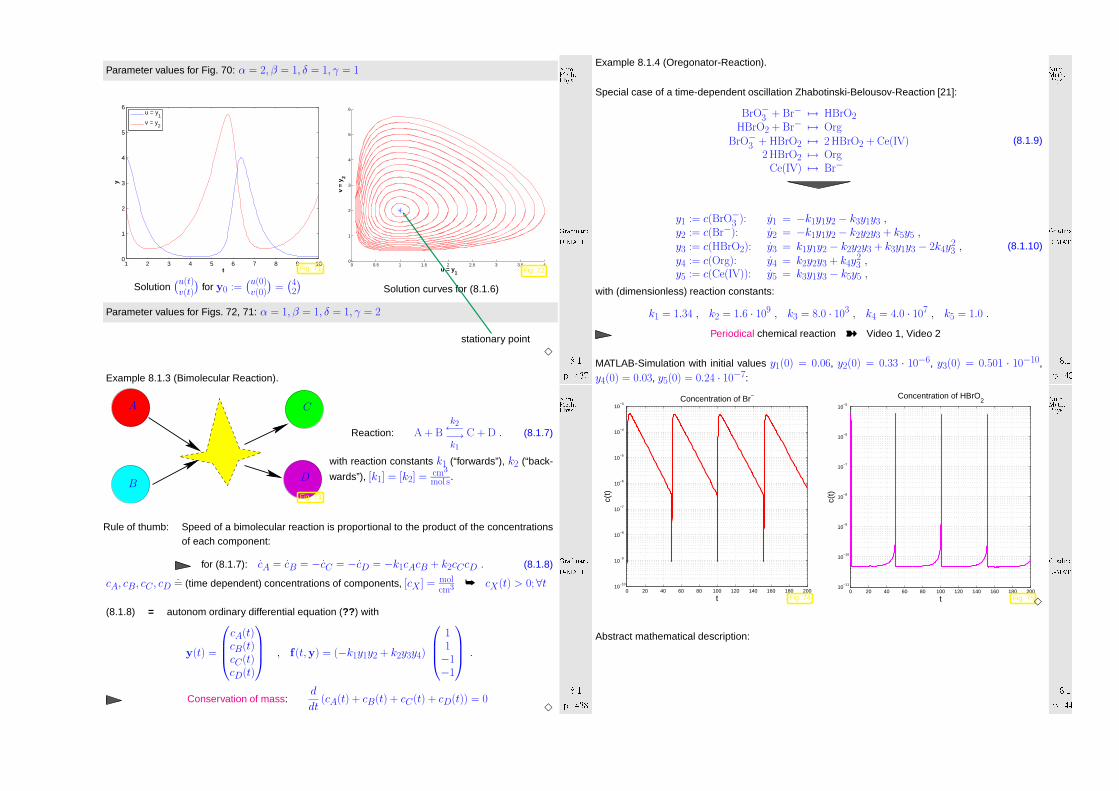
Parameter values for Fig. 70: α = 2, β = 1, δ = 1, γ = 1

1 2 3 4 5 6 7 8 9 100

1

2

3

4

5

6

t

y

u = y

1

v = y2

Fig. 71

Solution(u(t)v(t)

)for y0 :=

(u(0)v(0)

)=(42

)0 0.5 1 1.5 2 2.5 3 3.5 4

0

1

2

3

4

5

6

u = y1

v =

y2

Fig. 72

Solution curves for (8.1.6)

Parameter values for Figs. 72, 71: α = 1, β = 1, δ = 1, γ = 2

stationary point3

Example 8.1.3 (Bimolecular Reaction).


Num.Meth.Phys.

A

B

C

D

Fig. 73

Reaction: A + Bk2←−−→k1

C + D . (8.1.7)

with reaction constants k1 (“forwards”), k2 (“back-

wards”), [k1] = [k2] = cm3

mol s.

Rule of thumb: Speed of a bimolecular reaction is proportional to the product of the concentrationsof each component:

for (8.1.7): cA = cB = −cC = −cD = −k1cAcB + k2cCcD . (8.1.8)

cA, cB, cC , cD = (time dependent) concentrations of components, [cX ] = molcm3

cX(t) > 0; ∀t

(8.1.8) = autonom ordinary differential equation (?? ) with

y(t) =

cA(t)cB(t)cC(t)cD(t)

, f(t,y) = (−k1y1y2 + k2y3y4)

11−1−1

.

Conservation of mass:d

dt(cA(t) + cB(t) + cC(t) + cD(t)) = 0

3


Num.Meth.Phys.

Example 8.1.4 (Oregonator-Reaction).

Special case of a time-dependent oscillation Zhabotinski-Belousov-Reaction [21]:

BrO−3 + Br− 7→ HBrO2HBrO2 + Br− 7→ Org

BrO−3 + HBrO2 7→ 2 HBrO2 + Ce(IV)2 HBrO2 7→ Org

Ce(IV) 7→ Br−

(8.1.9)

y1 := c(BrO−3 ): y1 = −k1y1y2 − k3y1y3 ,y2 := c(Br−): y2 = −k1y1y2 − k2y2y3 + k5y5 ,y3 := c(HBrO2): y3 = k1y1y2 − k2y2y3 + k3y1y3 − 2k4y

23 ,

y4 := c(Org): y4 = k2y2y3 + k4y23 ,

y5 := c(Ce(IV)): y5 = k3y1y3 − k5y5 ,

(8.1.10)

with (dimensionless) reaction constants:

k1 = 1.34 , k2 = 1.6 · 109 , k3 = 8.0 · 103 , k4 = 4.0 · 107 , k5 = 1.0 .

Periodical chemical reaction Video 1, Video 2

MATLAB-Simulation with initial values y1(0) = 0.06, y2(0) = 0.33 · 10−6, y3(0) = 0.501 · 10−10,

y4(0) = 0.03, y5(0) = 0.24 · 10−7:


Num.Meth.Phys.

0 20 40 60 80 100 120 140 160 180 20010

−10

10−9

10−8

10−7

10−6

10−5

10−4

10−3

Concentration of Br−

tc(

t)Fig. 74

0 20 40 60 80 100 120 140 160 180 20010

−11

10−10

10−9

10−8

10−7

10−6

10−5

t

c(t)

Concentration of HBrO2

Fig. 753

Abstract mathematical description:


Num.Meth.Phys.

'

&

$

%

Initial value problem (IVP) for first-order ordinary differential equation (ODE): (→ [52,

Sect. 5.6])

y = f(t,y) , y(t0) = y0 . (8.1.11)

f : I ×D 7→ Rd = right hand side (r.h.s.) (d ∈ N), given in procedural form

function v = f(t,y).

I ⊂ R = (time)interval ↔ “time variable” t

D ⊂ Rd = state space/phase space ↔ “state variable” y (ger.: Zustandsraum)

Ω := I ×D = extended state space (of tupels (t,y))

t0 = initial time, y0 = initial state initial conditions

Terminology: f = f(y), r.h.s. does not depend on time y = f(y) is autonomous ODE

For autonomous ODEs: I = R and r.h.s. y 7→ f(y) can be regarded as stationary vector

field (velocity field)if t 7→ y(t) is solution ⇒ for any τ ∈ R t 7→ y(t + τ ) is solution,

too.initial time irrelevant: canonical choice t0 = 0


Num.Meth.Phys.

Note: autonomous ODEs naturally arise when modeling time-invariant systems/phenomena. All

examples above led to autonomous ODEs.

Remark 8.1.5 (Conversion into autonomous ODE).

Idea: include time as an extra d + 1-st component of an extended state vector.

This solution component has to grow linearly ⇔ temporal derivative = 1

z(t) :=

(y(t)t

)=

(z′

zd+1

): y = f(t,y) ↔ z = g(z) , g(z) :=

(f(zd+1, z

′)1

).

Remark 8.1.6 (From higher order ODEs to first order systems).

Ordinary differential equation of order n ∈ N:

y(n) = f(t,y, y, . . . ,y(n−1)) . (8.1.12)

Notation: superscript (n) = n-th temporal derivative t


Num.Meth.Phys.

Conversion into 1st-order ODE (system of size nd)

z(t) :=

y(t)

y(1)(t)...

y(n−1)(t)

=

z1z2...

zn

∈ R

dn: (8.1.12) ↔ z = g(z) , g(z) :=

z2z3...

znf(t, z1, . . . , zn)

.

(8.1.13)

Note: n initial values y(t0), y(t0), . . . ,y(n−1)(t0) required!

Basic assumption: right hand side f : I ×D 7→ Rd locally Lipschitz continuous in y

Defin ition 8.1.1 (Lipschitz continuous function). (→ [52, Def. 4.1.4])

f : Ω 7→ Rd is Lipschitz continuous (in the second argument), if

∃L > 0: ‖f(t,w)− f(t, z)‖ ≤ L ‖w − z‖ ∀(t,w), (y, z) ∈ Ω .

Defin ition 8.1.2 (Local Lipschitz continuity). (→ [52, Def. 4.1.5])d is locally Lipschitz continuous, if


Num.Meth.Phys.

Notation: Dyf = derivative of f w.r.t. state variable (= Jacobian ∈ Rd,d !)

A simple criterion for local Lipschitz continuity:

'

&

$

%

Lemma 8.1.3 (Criterion for local Liptschitz continuity).

If f and Dyf are continuous on the extended state space Ω, then f is locally Lipschitz

continuous(→ Def. 8.1.2).

'

&

$

%

Theorem 8.1.4 (Theorem of Peano & Picard-Lindelöf). [1, Satz II(7.6)], [52, Satz 6.5.1]

If f : Ω 7→ Rd is locally Lipschitz continuous (→ Def. 8.1.2) then for all initial conditions

(t0,y0) ∈ Ω the IVP (8.1.11) has a solution y ∈ C1(J(t0,y0), Rd) with maximal (temporal)

domain of definition J(t0,y0) ⊂ R.

Remark 8.1.7 (Domain of definition of solutions of IVPs).

Solutions of an IVP have an intrinsic maximal domain of definition


Num.Meth.Phys.

! domain of definition/domain of existence J(t0,y0) usually depends on (t0,y0) !

Terminology: if J(t0,y0) = I solution y : I 7→ Rd is global.

Notation: for autonomous ODE we always have t0 = 0, therefore write J(y0) := J(0,y0).

In light of Rem. 8.1.5 and Thm. 8.1.4: we consider only

autonomous IVP: y = f(y) , y(0) = y0 , (8.1.14)

with locally Lipschitz continuous (→ Def. 8.1.2) right hand side f .

Assumption 8.1.5 (Global solutions).

All solutions of (8.1.14) are global: J(y0) = R for all y0 ∈ D.


Num.Meth.Phys.

Change of perspective: fix “time of interest” t ∈ R \ 0

mapping Φt :

D 7→ Dy0 7→ y(t)

, t 7→ y(t) solution of IVP (8.1.14) ,

is well-defined mapping of the state space into itself, by Thm. 8.1.4 and Ass. 8.1.5

Now, we may also let t vary, which spawns a family of mappingsΦt

of the state space into itself.

However, it can also be viewed as a mapping with two arguments, a time t and an initial state value

y0!

Defin ition 8.1.6 (Evolution operator).

Under Assumption 8.1.5 the mapping

Φ :

R×D 7→ D(t,y0) 7→ Φty0 := y(t)

,

where t 7→ y(t) ∈ C1(R, Rd) is the unique (global) solution of the IVP y = f(y), y(0) = y0, is

the evolution operator for the ODE y = f(y).


Num.Meth.Phys.

Note: t 7→ Φty0 describes the solution of y = f(y) for y(0) = y0 (a trajectory)

Remark 8.1.8 (Group property of autonomous evolutions).

Under Assumption 8.1.5 the evolution operator gives rise to a group of mappings D 7→ D:

Φs Φt = Φs+t , Φ−t Φt = Id ∀t ∈ R . (8.1.15)

This is a consequence of the uniqueness theorem Thm. 8.1.4. It is also intuitive: following an evolution

up to time t and then for some more time s leads us to the same final state as observing it for the

whole time s + t.

8.2 Euler method s

Targeted: initial value problem (8.1.11)

y = f(t,y) , y(t0) = y0 . (8.1.11)


Num.Meth.Phys.

Sought: approximate solution of (8.1.11) on [t0, T ] up to final time T 6= t0

However, the solution of an initial value problem is a function J(t0,y0) 7→ Rd and requires a suitable

approximate representation. We postpone this issue here and first study a geometric approach to

numerical integration.

numerical integration = approximate solution of initial value problems for ODEs

(Please distinguish from “numerical quadrature”, see Ch. 7.)

Idea: ➊ timestepping: successive approximation of evolution on small intervals

[tk−1, tk], k = 1, . . . , N , tN := T ,

➋ approximation of solution on [tk−1, tk] by tangent curve to current initial

condition.


Num.Meth.Phys.

y(t)

t

y

t0 t1

y1

y0

Fig. 76

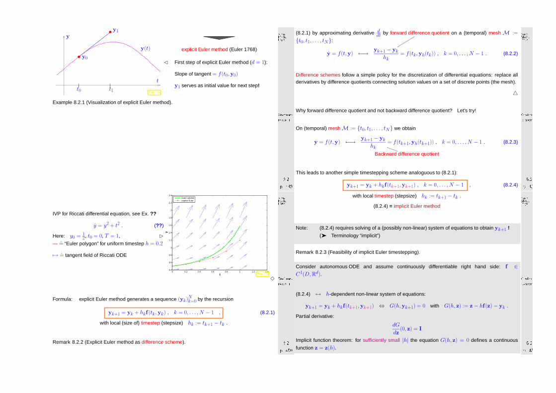
explicit Euler method (Euler 1768)

First step of explicit Euler method (d = 1):

Slope of tangent = f(t0,y0)

y1 serves as initial value for next step!

Example 8.2.1 (Visualization of explicit Euler method). GradinaruD-MATHp. 4498.2

Num.Meth.Phys.

IVP for Riccati differential equation, see Ex. ??

y = y2 + t2 . (?? )

Here: y0 = 12, t0 = 0, T = 1,

— = “Euler polygon” for uniform timestep h = 0.2

7→ = tangent field of Riccati ODE

0 0.2 0.4 0.6 0.8 1 1.2 1.40.4

0.6

0.8

1

1.2

1.4

1.6

1.8

2

2.2

2.4

t

y

exact solutionexplicit Euler

Fig. 77

3

Formula: explicit Euler method generates a sequence (yk)Nk=0 by the recursion

yk+1 = yk + hkf(tk,yk) , k = 0, . . . , N − 1 , (8.2.1)

with local (size of) timestep (stepsize) hk := tk+1 − tk .

Remark 8.2.2 (Explicit Euler method as difference scheme).


Num.Meth.Phys.

(8.2.1) by approximating derivative ddt by forward difference quotient on a (temporal) mesh M :=

t0, t1, . . . , tN:

y = f(t,y) ←→ yk+1 − yk

hk= f(tk,yh(tk)) , k = 0, . . . , N − 1 . (8.2.2)

Difference schemes follow a simple policy for the discretization of differential equations: replace allderivatives by difference quotients connecting solution values on a set of discrete points (the mesh).

Why forward difference quotient and not backward difference quotient? Let’s try!

On (temporal) meshM := t0, t1, . . . , tN we obtain

y = f(t,y) ←→ yk+1 − yk

hk= f(tk+1,yh(tk+1)) , k = 0, . . . , N − 1 . (8.2.3)

Backward difference quotient

This leads to another simple timestepping scheme analoguous to (8.2.1):

yk+1 = yk + hkf(tk+1,yk+1) , k = 0, . . . , N − 1 , (8.2.4)


Num.Meth.Phys.

with local timestep (stepsize) hk := tk+1 − tk .

(8.2.4) = implicit Euler method

Note: (8.2.4) requires solving of a (possibly non-linear) system of equations to obtain yk+1 !

( Terminology “implicit”)

Remark 8.2.3 (Feasibility of implicit Euler timestepping).

Consider autonomous ODE and assume continuously differentiable right hand side: f ∈C1(D, Rd).

(8.2.4) ↔ h-dependent non-linear system of equations:

yk+1 = yk + hkf(tk+1,yk+1) ⇔ G(h,yk+1) = 0 with G(h, z) := z− hf(z)− yk .

Partial derivative:

dG

dz(0, z) = I

Implicit function theorem: for sufficiently small |h| the equation G(h, z) = 0 defines a continuous

function z = z(h).


Num.Meth.Phys.

How to interpret the sequence (yk)Nk=0 from (8.2.1)?

By “geometric insight” we expect: yk ≈ y(tk)

(Throughout, we use the notation y(t) for the exact solution of an IVP.)

If we are merely interested in the final state y(T ), then the explicit Euler method will give us theanswer yN .

If we are interested in an approximate solution yh(t) ≈ y(t) as a function [t0, T ] 7→ Rd, we have to

do

post-processing = reconstruction of a function from yk, k = 0, . . . , N

Technique: interpolation, see Ch. 5

Simplest option: piecewise linear interpolation (→ Sect. ?? ) Euler polygon, see Fig. 77.


Num.Meth.Phys.

Abstract sing le step method s

Recall Euler methods for autonomous ODE y = f(y):

explicit Euler: yk+1 = yk + hkf(yk) ,

implicit Euler: yk+1: yk+1 = yk + hkf(yk+1) .

Both formulas provide a mapping

(yk, hk) 7→ Ψ(h,yk) := yk+1 . (8.2.5)

Recall the interpretation of the yk as approximations of y(tk):

Ψ(h,y) ≈ Φhy , (8.2.6)

where Φ is the evolution operator (→ Def. 8.1.6) for y = f(y).

The Euler methods provide approximations for evolution operator for ODEs

This is what every single step method does: it tries to approximate the evolution operator Φ for an

ODE by a mapping of the type (8.2.5).

mapping Ψ from (8.2.5) is called discrete evolution.

Vice versa: a mapping Ψ as in (8.2.5) defines a single step method.


Num.Meth.Phys.

In a sense, a single step method defined through its associated discrete evolution does not

approximate and initial value problem, but tries to approximate an ODE.

Defin ition 8.2.1 (Single step method (for autonomous ODE)).

Given a discrete evolution Ψ : Ω ⊂ R × D 7→ Rd, an initial state y0, and a temporal mesh

M := t0 < t1 < · · · < tN = T the recursion

yk+1 := Ψ(tk+1 − tk,yk) , k = 0, . . . , N − 1 , (8.2.7)

defines a single step method (SSM, ger.: Einschrittverfahren) for the autonomous IVP y = f(y),

y(0) = y0.

Procedural view of discrete evolutions:

Ψhy ←→ function y1 = esvstep(h,y0) .

( function y1 = esvstep( rhs,h,y0) )


Num.Meth.Phys.

Notation: Ψhy := Ψ(h,y)

Concept of single step method according to Def. 8.2.1 can be generalized to non-autonomous ODEs,

which leads to recursions of the form:

yk+1 := Ψ(tk, tk+1,yk) , k = 0, . . . , N − 1 ,

for discrete evolution defined on I × I ×D.

Remark 8.2.4 (Notation for single step methods).

Many authors specify a single step method by writing down the first step:

y1 = expression in y0 and f .

Also this course will sometimes adopt this practice.


Num.Meth.Phys.

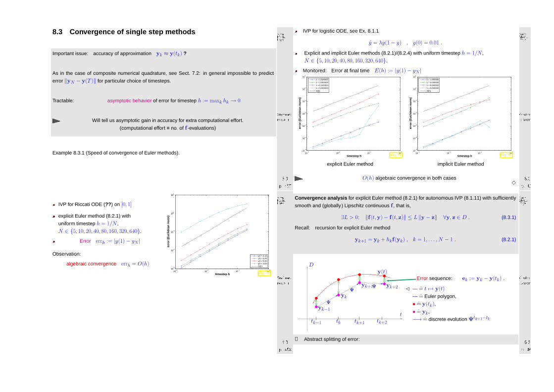
8.3 Convergence of sing le step method s

Important issue: accuracy of approximation yk ≈ y(tk) ?

As in the case of composite numerical quadrature, see Sect. 7.2: in general impossible to predict

error ‖yN − y(T )‖ for particular choice of timesteps.

Tractable: asymptotic behavior of error for timestep h := maxk hk → 0

Will tell us asymptotic gain in accuracy for extra computational effort.

(computational effort = no. of f -evaluations)

Example 8.3.1 (Speed of convergence of Euler methods).


Num.Meth.Phys.

IVP for Riccati ODE (?? ) on [0, 1]

explicit Euler method (8.2.1) with

uniform timestep h = 1/N ,

N ∈ 5, 10, 20, 40, 80, 160, 320, 640.Error errh := |y(1)− yN |

Observation:

algebraic convergence errh = O(h)10

−310

−210

−110

010

−3

10−2

10−1

100

101

timestep h

err

or (

Euc

lidea

n no

rm)

y0 = 0.10y0 = 0.20y0 = 0.40y0 = 0.80O(h)

Fig. 78 GradinaruD-MATHp. 4588.3

Num.Meth.Phys.

IVP for logistic ODE, see Ex. 8.1.1

y = λy(1− y) , y(0) = 0.01 .

Explicit and implicit Euler methods (8.2.1)/(8.2.4) with uniform timestep h = 1/N ,

N ∈ 5, 10, 20, 40, 80, 160, 320, 640.Monitored: Error at final time E(h) := |y(1)− yN |

10−3

10−2

10−1

100

10−5

10−4

10−3

10−2

10−1

100

101

timestep h

err

or (

Euc

lidea

n no

rm)

λ = 1.000000λ = 3.000000λ = 6.000000λ = 9.000000O(h)

Fig. 79

explicit Euler method

10−3

10−2

10−1

100

10−5

10−4

10−3

10−2

10−1

100

101

timestep h

err

or (

Euc

lidea

n no

rm)

λ = 1.000000λ = 3.000000λ = 6.000000λ = 9.000000O(h)

Fig. 80

implicit Euler method

O(h) algebraic convergence in both cases3


Num.Meth.Phys.

Convergence analys is for explicit Euler method (8.2.1) for autonomous IVP (8.1.11) with sufficiently

smooth and (globally) Lipschitz continuous f , that is,

∃L > 0: ‖f(t,y)− f(t, z)‖ ≤ L ‖y − z‖ ∀y, z ∈ D . (8.3.1)

Recall: recursion for explicit Euler method

yk+1 = yk + hkf(yk) , k = 1, . . . , N − 1 . (8.2.1)

tk−1 tk tk+1 tk+2

yk−1

yk

yk+1 yk+2

D

t

y(t)

Ψ

ΨΨ

Error sequence: ek := yk − y(tk) .

— = t 7→ y(t)

— = Euler polygon,

• = y(tk),

• = yk,

−→ = discrete evolution Ψtk+1−tk

➀ Abstract splitting of error:


Num.Meth.Phys.

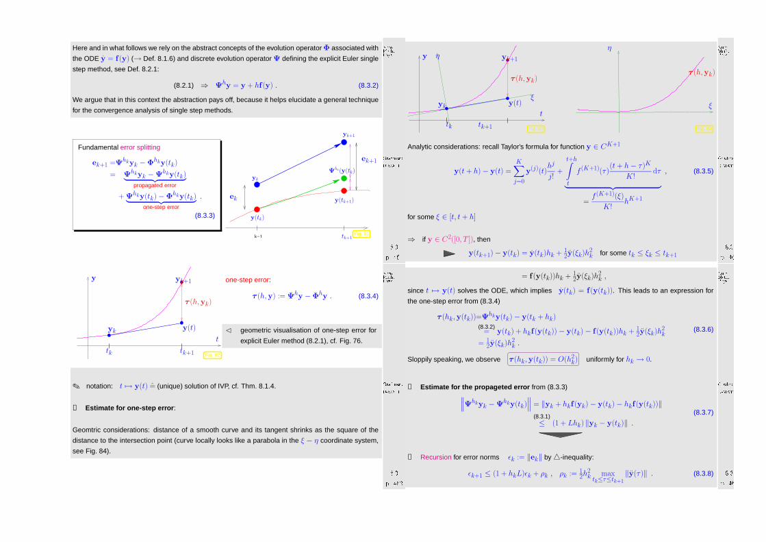
Here and in what follows we rely on the abstract concepts of the evolution operator Φ associated with

the ODE y = f(y) (→ Def. 8.1.6) and discrete evolution operator Ψ defining the explicit Euler single

step method, see Def. 8.2.1:

(8.2.1) ⇒ Ψhy = y + hf(y) . (8.3.2)

We argue that in this context the abstraction pays off, because it helps elucidate a general technique

for the convergence analysis of single step methods.

Fundamental error splitting

ek+1 =Ψhkyk −Φhky(tk)

= Ψhkyk −Ψhky(tk)︸︷︷︸propagated error

+ Ψhky(tk)−Φhky(tk)︸︷︷︸one-step error

.

(8.3.3)

k−1

y(tk)

y(tk+1)

Ψhk(y(tk)yk

yk+1

ek

ek+1

tk+1Fig. 81


Num.Meth.Phys.y(t)

t

y

tk tk+1

yk+1

yk

τ (h,yk)

Fig. 82

one-step error:

τ (h,y) := Ψhy −Φhy . (8.3.4)

geometric visualisation of one-step error for

explicit Euler method (8.2.1), cf. Fig. 76.

notation: t 7→ y(t) = (unique) solution of IVP, cf. Thm. 8.1.4.

➁ Estimate for one-step error:

Geomtric considerations: distance of a smooth curve and its tangent shrinks as the square of the

distance to the intersection point (curve locally looks like a parabola in the ξ − η coordinate system,

see Fig. 84).


Num.Meth.Phys.

ξ

η

y(t)

t

y

tk tk+1

yk+1

yk

τ (h,yk)

Fig. 83

ξ

η

τ (h,yk)

Fig. 84

Analytic considerations: recall Taylor’s formula for function y ∈ CK+1

y(t + h)− y(t) =K∑

j=0

y(j)(t)hj

j!+

t+h∫

t

f (K+1)(τ )(t + h− τ )K

K!dτ

︸︷︷︸

=f (K+1)(ξ)

K!hK+1

, (8.3.5)

for some ξ ∈ [t, t + h]

⇒ if y ∈ C2([0, T ]), then

y(tk+1)− y(tk) = y(tk)hk + 12y(ξk)h2

k for some tk ≤ ξk ≤ tk+1


Num.Meth.Phys.

= f(y(tk))hk + 12y(ξk)h2

k ,

since t 7→ y(t) solves the ODE, which implies y(tk) = f(y(tk)). This leads to an expression for

the one-step error from (8.3.4)

τ (hk,y(tk))=Ψhky(tk)− y(tk + hk)(8.3.2)

= y(tk) + hkf(y(tk))− y(tk)− f(y(tk))hk + 12y(ξk)h2

k

= 12y(ξk)h2

k .

(8.3.6)

Sloppily speaking, we observe τ (hk,y(tk)) = O(h2k) uniformly for hk → 0.

➂ Estimate for the propageted error from (8.3.3)∥∥∥Ψhkyk −Ψhky(tk)

∥∥∥ = ‖yk + hkf(yk)− y(tk)− hkf(y(tk))‖(8.3.1)≤ (1 + Lhk) ‖yk − y(tk)‖ .

(8.3.7)

➂ Recursion for error norms ǫk := ‖ek‖ by-inequality:

ǫk+1 ≤ (1 + hkL)ǫk + ρk , ρk := 12h

2k max

tk≤τ≤tk+1

‖y(τ )‖ . (8.3.8)


Num.Meth.Phys.

Taking into account ǫ0 = 0 this leads to

ǫk ≤k∑

l=1

l−1∏

j=1

(1 + Lhj) ρl , k = 1, . . . , N . (8.3.9)

Use the elementary estimate (1 + Lhj) ≤ exp(Lhj) (by convexity of exponential function):

(8.3.9) ⇒ ǫk ≤k∑

l=1

l−1∏

j=1

exp(Lhj) · ρl =k∑

l=1

exp(L∑l−1

j=1hj)ρl .

Note:l−1∑j=1

hj ≤ T for final time T

ǫk ≤ exp(LT )k∑

l=1

ρl ≤ exp(LT ) maxk

ρk

hk

k∑

l=1

hl

≤ T exp(LT ) maxl=1,...,k

hl · maxt0≤τ≤tk

‖y(τ )‖ .

‖yk − y(tk)‖ ≤ T exp(LT ) maxl=1,...,k

hl · maxt0≤τ≤tk

‖y(τ )‖ .


Num.Meth.Phys.

Total error arises from accumulation of one-step errors!

error bound = O(h), h := maxl

hl ( 1st-order algebraic convergence)

Error bound grows exponentially with the length T of the integration interval.

Most commonly used single step methods display algebraic convergence of integer order with respect

to the meshwidth h := maxk hk. This offers a criterion for gauging their quality.

The sequence (yk)k generated by a

single step method (→ Def. 8.2.1) of order (of consistency) p ∈ N

for y = f(t,y) on a meshM := t0 < t1 < · · · < tN = T satisfies

maxk‖yk − y(tk)‖ ≤ Chp for h := max

k=1,...,N|tk − tk−1| → 0 ,

with C > 0 independent ofM, provided that f is sufficiently smooth.


Num.Meth.Phys.

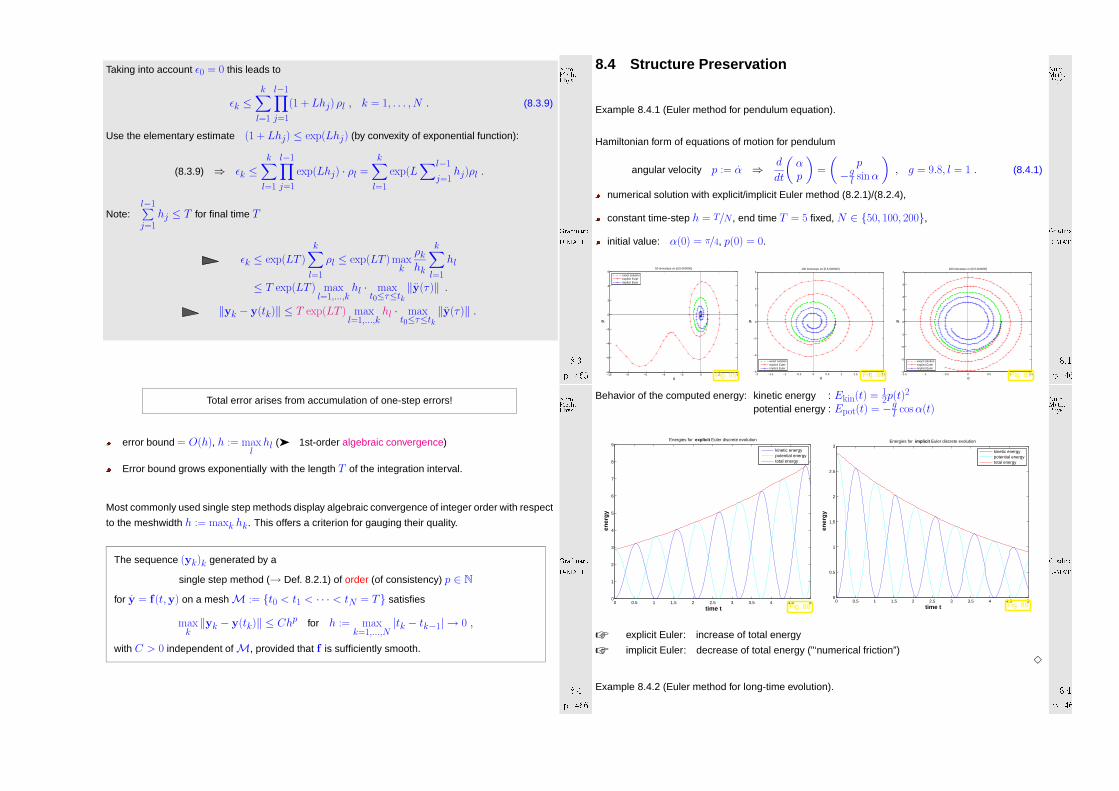
8.4 Structure Preservation

Example 8.4.1 (Euler method for pendulum equation).

Hamiltonian form of equations of motion for pendulum

angular velocity p := α ⇒ d

dt

(αp

)=

(p

−gl sin α

), g = 9.8, l = 1 . (8.4.1)

numerical solution with explicit/implicit Euler method (8.2.1)/(8.2.4),

constant time-step h = T/N , end time T = 5 fixed, N ∈ 50, 100, 200,

initial value: α(0) = π/4, p(0) = 0.

−10 −8 −6 −4 −2 0 2 4−8

−6

−4

−2

0

2

4

6

α

p

50 timesteps on [0,5.000000]

exact solutionexplicit Eulerimplicit Euler

Fig. 85 −2 −1.5 −1 −0.5 0 0.5 1 1.5 2 2.5−6

−4

−2

0

2

4

6

α

p

100 timesteps on [0,5.000000]


Fig. 86 −1.5 −1 −0.5 0 0.5 1 1.5−4

−3

−2

−1

0

1

2

3

4

α

p

200 timesteps on [0,5.000000]


Fig. 87


Num.Meth.Phys.

Behavior of the computed energy: kinetic energy : Ekin(t) = 12p(t)2

potential energy : Epot(t) = −gl cos α(t)

0 0.5 1 1.5 2 2.5 3 3.5 4 4.5 50

1

2

3

4

5

6

7

8

9

time t e

nerg

y

Energies for explicit Euler discrete evolution

kinetic energypotential energytotal energy

Fig. 880 0.5 1 1.5 2 2.5 3 3.5 4 4.5 5

0

0.5

1

1.5

2

2.5

3

time t

ene

rgy

Energies for implicit Euler discrete evolution


Fig. 89

explicit Euler: increase of total energy

implicit Euler: decrease of total energy ("‘numerical friction”)3

Example 8.4.2 (Euler method for long-time evolution).


Num.Meth.Phys.

Initial value problem for , D = R2:

y =

(y2−y1

), y(0) = y0 y(t) =

(cos t sin t− sin t cos t

)y0 .

Note that I(y) = ‖y‖ is constant.

(movement with constant velocity on the circle)

−4 −3 −2 −1 0 1 2 3−3

−2.5

−2

−1.5

−1

−0.5

0

0.5

1

1.5

2

y1

y2

40 timesteps on [0,10.000000]


Fig. 90−1.5 −1 −0.5 0 0.5 1 1.5

−1.5

−1

−0.5

0

0.5

1

1.5

y1

y2

160 timesteps on [0,10.000000]


Fig. 91

explicit Euler: numerical solution flyes away

implicit Euler: numerical solution falls off into the center3


Num.Meth.Phys.

8.4.1 Implicit Midpo int Rule

Can we avoid the energy drift ?

t

y

t0 t1

yh(t1)

y0

y∗

t∗

f(t∗,y∗)

Fig. 92

Idea: Approximate solution through (t0,y0) on

[t0, t1] via

• linear polynomial through (t0,y0)

• with slope f(t∗,y∗),t∗ := 1

2(t0 + t1), y∗ = 1

2(y0 + y1)

— = solution through (t0, y0),

— = solution through (t∗, y∗),— = tangent at — in (t∗, y∗).

Apply on small time intervals [t0, t1], [t1, t2], . . ., [tN−1, tN ] implicit midpoint rule

via implicit midpoint rule generated approximation yk+1 for y(tk) fulfils

yk+1 := yh(tk+1) = yk + hkf(12(tk + tk+1),

12(yk + yk+1)) , k = 0, . . . , N − 1 , (8.4.2)

with local (Time)step hk := tk+1 − tk .


Num.Meth.Phys.

Note: (8.4.2) requires soltion of a (evtl. non-linear) equation for yk+1 !

( "‘implicit”)

Remark 8.4.3 (Implicit midpoint rule as difference method).

(8.4.2) from the approximation of time-derivative ddt via centred difference quotients on time-grid G :=

t0, t1, . . . , tN:

y = f(t,y) ←→ yh(tk+1)− yh(tk)

hk= f(1

2(tk + tk+1),12(yh(tk) + y(tk+1)), k = 0, . . . , N − 1 .

Example 8.4.4 (Implicit midpoint rule for logistic equation). GradinaruD-MATHp. 4718.4

Num.Meth.Phys.

10−3

10−2

10−1

100

10−9

10−8

10−7

10−6

10−5

10−4

10−3

10−2

10−1

100

timestep h

err

or (

Euc

lidea

n no

rm)

λ = 1.000000λ = 2.000000λ = 5.000000λ = 10.000000

O(h2)

Fig. 93

λ small: O(h2)-convergence (asymptotical)

10−3

10−2

10−1

100

10−16

10−14

10−12

10−10

10−8

10−6

10−4

10−2

100

timestep h

err

or (

Euc

lidea

n no

rm)

λ = 10.000000λ = 20.000000λ = 50.000000λ = 90.000000

O(h2)

Fig. 94

λ large: stable for all time steps h !3

Example 8.4.5 (Implicit midpoint rule for circular motion).


Num.Meth.Phys.

−4 −3 −2 −1 0 1 2 3−3

−2.5

−2

−1.5

−1

−0.5

0

0.5

1

1.5

2

y1

y2

40 timesteps on [0,10.000000]

exact solutionexplicit Eulerimplicit Eulerimplicit midpoint

Fig. 95−1.5 −1 −0.5 0 0.5 1 1.5

−1.5

−1

−0.5

0

0.5

1

1.5

y1

y2

160 timesteps on [0,10.000000]


Fig. 96

Implicit midpoint rule: perfect conservation of length !3

Example 8.4.6 (Implicit midpoint rule for pendulum).

Initial values and problem as in Bsp. 8.4.1


Num.Meth.Phys.−10 −8 −6 −4 −2 0 2 4

−8

−6

−4

−2

0

2

4

6

α

p

50 timesteps on [0,5.000000]


Fig. 97 −2 −1.5 −1 −0.5 0 0.5 1 1.5 2 2.5−6

−4

−2

0

2

4

6

α

p

100 timesteps on [0,5.000000]


Fig. 98 −1.5 −1 −0.5 0 0.5 1 1.5−4

−3

−2

−1

0

1

2

3

4

α

p

200 timesteps on [0,5.000000]


Fig. 99

0 0.5 1 1.5 2 2.5 3 3.5 4 4.5 50

0.5

1

1.5

2

2.5

3

time t

ene

rgy

Energies for implicit midpoint discrete evolution


Fig. 100

Behavior of the energy of the numerical solu-

tion computed with the midpoint rule (8.4.2),

N = 50.

No energy drift although large time step)

3


Num.Meth.Phys.

8.4.2 Störmer-Verlet Method [?]

?use the idea of Euler method for an equation of 2nd order

y = f(t,y) . (8.4.3)

Given yk−1 ≈ y(tk−1), yk ≈ y(tk) approximate y(t) on [tk−1, tk+1] via

• parabola p(t) through (tk−1,yk−1), (tk,yk) (∗),• with p(tk) = f(yk) (∗).

(∗) Parabola is uniquely determined.

yk+1 := p(tk+1) ≈ y(tk+1)

Störmer-Verlet method for (8.4.3) (time-grid G := t0, t1, . . . , tN):

yk+1 = − hk

hk−1yk−1 +

(1 +

hk

hk−1

)yk + 1

2(h2k + hkhk−1)f(tk,yk) , k = 1, . . . , N − 1 .

(8.4.4)

In case of a fixed time step h:

yk+1 = −yk−1 + 2yk + h2f(tk,yk) , k = 1, . . . , N − 1 . (8.4.5)


Num.Meth.Phys.

Note: (8.4.4) does not require the solution of an equation ( explicit method)

We say: yk+1 = yk+1(yk,yk−1) (8.4.4) is a two-step method

(explicit/implicit Euler method, midpoint rule = one-step method)

Remark 8.4.7 (Störmer-Verlet method as difference method).

(8.4.5) from the approximation of the second time-derivative by a

second centered difference quotients on time-grid G := t0, t1, . . . , tN: for cosntant time-step

h > 0

y = f(y) ←→yh(tk+1)−yh(tk)

h − yh(tk)−yh(tk−1)h

h=

yh(tk+1)− 2yh(tk) + yh(tk−1)

h2

= f(yh(tk)) .

Remark 8.4.8 (Initialisation of the Störmer-Verlet method).

Initial values for (8.4.3)y(0) = y0, y(0) = v0


Num.Meth.Phys.

use virtual moment t−1 := t0 − h0

apply (8.4.5) to [t−1, t1]:

y1 = −y−1 + 2y0 + h20f(t0,y0) . (8.4.6)

centered difference quotient on [t−1, t1]:

y1 − y−1

2h0= v0 . (8.4.7)

compute y1 from (8.4.6) & (8.4.7)

Example 8.4.9 (Störmer-Verlet method for pendulum). GradinaruD-MATHp. 4778.4

Num.Meth.Phys.

(8.4.5)

initialisation via. 8.4.8

constant time step h := T/N , N ∈ N time

steps

reference solution via very precise integration

ode45()

α0 = π/2, p0 = 0, T = 5, vgl. Bsp. 8.4.1

Number of time steps: N = 40−2 −1.5 −1 −0.5 0 0.5 1 1.5 2

−5

−4

−3

−2

−1

0

1

2

3

4

5

angle α

vel

ocity

p

Pendulum g = 9.800000, l = 1.000000,α(0)=1.570796,p(0)=0.000000


Num.Meth.Phys.

0 0.5 1 1.5 2 2.5 3 3.5 4 4.5 5−2

−1.5

−1

−0.5

0

0.5

1

1.5

2

time t

ang

le α

Pendulum g = 9.800000, l = 1.000000,α(0)=1.570796,p(0)=0.000000

Fig. 102 0 0.5 1 1.5 2 2.5 3 3.5 4 4.5 5−5

−4

−3

−2

−1

0

1

2

3

4

5

time t

vel

ocity

p

Pendulum g = 9.800000, l = 1.000000,α(0)=1.570796,p(0)=0.000000


Num.Meth.Phys.

0 0.5 1 1.5 2 2.5 3 3.5 4 4.5 50

1

2

3

4

5

6

7

8

9

10

time t

ene

rgy

Energies for Stoermer−Verlet discrete evolution


Fig. 104

No energy drift thought large time steps

perfect periodical orbits !

On the contrary: Ex. 8.4.1

3

Remark 8.4.10 (One-step formulation of the Störmer-Verlet method).

In case of constant time step, see (8.4.5), analogously to the refromulation of a 2nd order equation to


Num.Meth.Phys.

a fisrt order equation, see (8.1.13): with vk+1

2

:=yk+1−yk

h

y = f(y) ←→ y = v ,v = f(y) .

l l

yk+1 − 2yk + yk−1 = h2kf(yk) ←→

vk+1

2

= vk + h2f(yk) ,

yk+1 = yk + hvk+1

2

,

vk+1 = vk+1

2

+ h2f(yk+1) .

two-steps method one-step method

Initialisation (→ Rem. 8.4.8) is built in already in the formulation.

Remark 8.4.11 (Störmer-Verlet method as polygonal line method).


Num.Meth.Phys.

Perspective: Störmer-Verlet method as

polygonal line method

(see Ren. 8.4.10)

vk+1

2

= vk−1

2

+ hf(yk) ,

yk+1 = yk + hvk+1

2

.

t

y/v

tk−2 tk−1 tk tk+1

f

f

yk−2

yk−1

yk

yk+1

vk−3/2

vk−1/2

vk+1/2

"Why so many different numerical methods for ODEs?”

Answer: each numerical integrator has its specific properties

best (not) suited for certain classes of initial value problems


Num.Meth.Phys.

8.4.3 Examples

Example 8.4.12 (Energy conservation). ↔ Bsp. 8.4.6

Pendulum IVP (8.4.1) on [0, 1000], p(0) = 0, q(0) = 7π/6.

Compare classical Runge-Kutta method (8.6.6) (order 4) with implicit midpoint rule 8.4.2), constanttime-step h = 1

2:

−2 −1.5 −1 −0.5 0 0.5 1 1.5 23

4

5

6

7

8

9

p

q

(p(t),q(t))RK4 MethodeImpl. Mittelpunktsregel

Fig. 105

Trajectories of "‘exact” /discrete evolutions

0 200 400 600 800 10000.55

0.6

0.65

0.7

0.75

0.8

0.85

0.9

0.95

t

Ges

amte

nerg

ie

RK4−MethodeImpl. Mittelpunktsregel

Fig. 106

Energy conservation of discrete evolutions


Num.Meth.Phys.

No drift in enrgy in case of midpoint rule

3

?Fascinating observation#

"

!Some (∗) numerical time-integrators:

approximative long-time energy conservation (no energy drift)

(∗) Implicit midpoint rule (8.4.2)→ Ex. 8.4.12, 8.4.6,

Störmer-Verlet mehtod (?? )→ Ex. 8.4.9

Example 8.4.13 (Spring-pendulum).

Friction-free spring-pendulum: Hamilton function (energy) H(p,q) = 12 ‖p‖

2 + 12(‖q‖ − 1)2 + q2

(q = position, p = momentum)

p = −(‖q‖ − 1)q

‖q‖ −(

0

1

), q = p . (8.4.8)


Num.Meth.Phys.

Fig. 107

Trajectories for long-time evolution

(chaotical mechanical system)−1 −0.8 −0.6 −0.4 −0.2 0 0.2 0.4 0.6 0.8 1

−3.5

−3

−2.5

−2

−1.5

−1

−0.5

0

q1

q2

Spring pendulum trajectory

Fig. 108

ESV: Störmer-Verlet method (8.4.5) (order 2),

explicit trapezoidal rule (8.6.3) (order 2).


Num.Meth.Phys.−1.5 −1 −0.5 0 0.5 1 1.5

−3.5

−3

−2.5

−2

−1.5

−1

−0.5

0

0.5

1

q1

q2

Stoermer−Verlet, h = 0.200000

0 < t < 501000 < t < 1050

Fig. 109

Störmer-Verlet

−1.5 −1 −0.5 0 0.5 1 1.5−3.5

−3

−2.5

−2

−1.5

−1

−0.5

0

0.5

1

q1

q2

Explicit trapezoidal rule, h = 0.200000

0 < t < 501000 < t < 1050

Fig. 110

Explicit trapezoidal rule

Störmer-Verlet: positions in “allowed domain” even for long times

Explicit trapezoidal rule: trajectories leave the “allowed domain” at long times (energy drift !)

3

Example 8.4.14 (Molecular dynamics). → [13, Sect. 1.2]


Num.Meth.Phys.

Space of states for n ∈ N atoms in d ∈ N dimensions: D = R2dn

(positions q = [q1; . . . ;qn]T ∈ Rdn, Momenta p = [p1, . . . ,pn]T ∈ R

dn)

Energy (Hamilton-function):

H(p,q) = 12 ‖p‖

22 + V (q) .

Lenard-Jones-potential:

V (q) =n∑

j=1

∑

i 6=j

V(∥∥∥qi − qj

∥∥∥2) ,

V(ξ) = ξ−12 − ξ−6 . (8.4.9)

0 0.5 1 1.5 2 2.5 3−0.5

0

0.5

1

1.5

2

2.5

3

|q|

H(q

)

Lenard−Jones potentialequilibrium distance

Fig. 111

Hamiltonian ODE

pj = −∑

i 6=j

V ′(∥∥∥qj − qi

∥∥∥2)

qj − qi∥∥qj − qi

∥∥2

, qj = pj , j = 1, . . . , n .

Störmer-Verlet method (8.4.5):

qh(t + 12h) = qh(t) + h

2ph(t) ,


Num.Meth.Phys.

pjh(t + h) = p

jh(t)− h

∑

i 6=j

V ′(∥∥∥qj

h(t + 12h)− qi

h(t + 12h)∥∥∥

2)

qjh(t + 1

2h)− qih(t + 1

2h)∥∥∥qjh(t + 1

2h)− qih(t + 1

2h)∥∥∥

2

,

qh(t + h) = qh(t + 12h) + h

2ph(t + h) .

Simulation with d = 2, n = 3, q1(0) = 12

√2(−1−1

), q2(0) = 1

2

√2(11

), q3(0) = 1

2

√2(−1

1

), p(0) = 0,

end-time T = 100

−1.5 −1 −0.5 0 0.5 1 −2

0

2

0

20

40

60

80

100

t

Trajektorien der Atome, Verlet, 10000 timesteps

x1

x2 0 10 20 30 40 50 60 70 80 90 100

−0.8

−0.6

−0.4

−0.2

0

0.2

0.4

0.6Energieanteile, Verlet, 10000 timesteps

t

E

kinetische Energiepotentielle EnergieGesamtenergie GradinaruD-MATH

p. 4888.4Num.Meth.Phys.

−2 −1.5 −1 −0.5 0 0.5 1 1.5 −2

0

2

0

20

40

60

80

100

t

Trajektorien der Atome, Verlet, 2000 timesteps

x1

x2 0 10 20 30 40 50 60 70 80 90 100

−0.8

−0.6

−0.4

−0.2

0

0.2

0.4

0.6Energieanteile, Verlet, 2000 timesteps

t

E

kinetische Energiepotentielle EnergieGesamtenergie

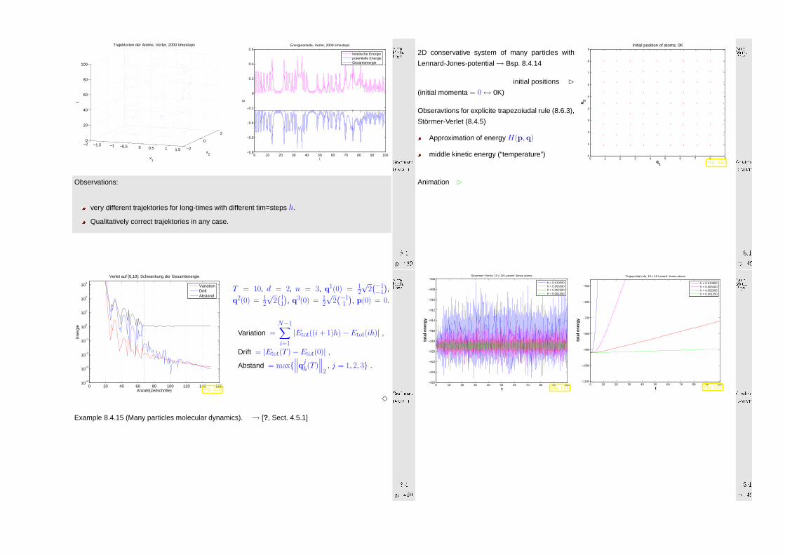
Observations:

very different trajektories for long-times with different tim=steps h.

Qualitatively correct trajektories in any case.


Num.Meth.Phys.0 20 40 60 80 100 120 140 160

10−4

10−3

10−2

10−1

100

101

102

103

Verlet auf [0,10]: Schwankung der Gesamtenergie

Anzahl(Zeitschritte)

Ene

rgie

VariationDriftAbstand

Fig. 112

T = 10, d = 2, n = 3, q1(0) = 12

√2(−1−1

),

q2(0) = 12

√2(11

), q3(0) = 1

2

√2(−1

1

), p(0) = 0.

Variation =N−1∑

i=1

|Etot((i + 1)h)− Etot(ih)| ,

Drift = |Etot(T )− Etot(0)| ,Abstand = max

∥∥∥qjh(T )

∥∥∥2, j = 1, 2, 3 .

3

Example 8.4.15 (Many particles molecular dynamics). → [?, Sect. 4.5.1]


Num.Meth.Phys.

2D conservative system of many particles with

Lennard-Jones-potential→ Bsp. 8.4.14

initial positions

(initial momenta = 0↔ 0K)

Obseravtions for explicite trapezoiudal rule (8.6.3),

Störmer-Verlet (8.4.5)

Approximation of energy H(p,q)

middle kinetic energy (“temperature”)0 1 2 3 4 5 6 7 8 9

0

1

2

3

4

5

6

7

8

9

q1

q2

Initial position of atoms, 0K

Fig. 113

Animation


Num.Meth.Phys.

0 10 20 30 40 50 60 70 80 90 100−926

−924

−922

−920

−918

−916

−914

−912

−910

−908

−906

t

tota

l ene

rgy

Stoermer−Verlet: 10 x 10 Lenard−Jones atoms

h = 0.010000h = 0.005000h = 0.002500h = 0.001250

Fig. 1140 10 20 30 40 50 60 70 80 90 100

−1100

−1000

−900

−800

−700

−600

−500

t

tota

l ene

rgy

Trapezoidal rule, 10 x 10 Lenard−Jones atoms

h = 0.010000h = 0.005000h = 0.002500h = 0.001250


Num.Meth.Phys.

0 10 20 30 40 50 60 70 80 90 1000

0.2

0.4

0.6

0.8

1

1.2

1.4

t

tem

pera

ture

Stoermer−Verlet: 10 x 10 Lenard−Jones atoms

h = 0.010000h = 0.005000h = 0.002500h = 0.001250

Fig. 1160 10 20 30 40 50 60 70 80 90 100

0

0.5

1

1.5

2

2.5

3

t

tem

pera

ture

Trapezoidal rule, 10 x 10 Lenard−Jones atoms

h = 0.010000h = 0.005000h = 0.002500h = 0.001250

Fig. 117

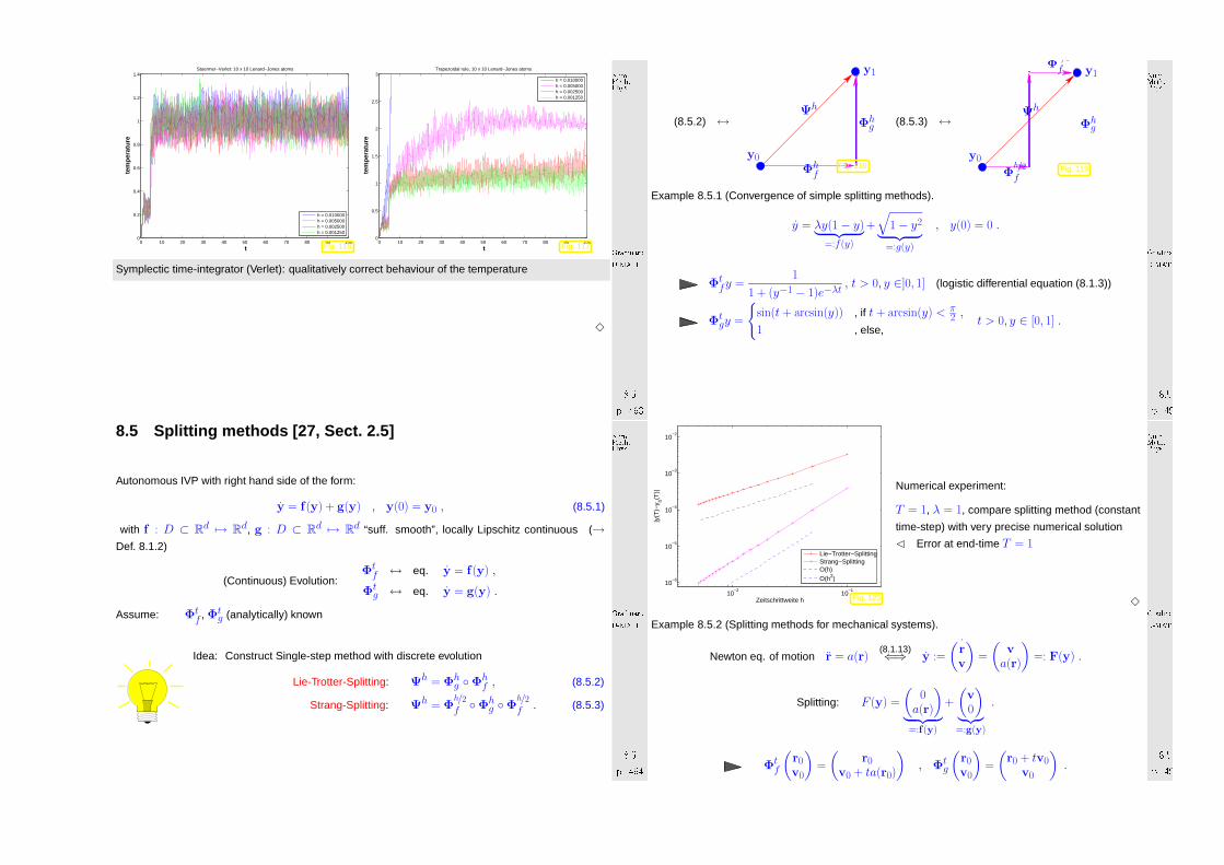
Symplectic time-integrator (Verlet): qualitatively correct behaviour of the temperature

3


Num.Meth.Phys.

8.5 Spli tt ing method s [27, Sect. 2.5]

Autonomous IVP with right hand side of the form:

y = f(y) + g(y) , y(0) = y0 , (8.5.1)

with f : D ⊂ Rd 7→ R

d, g : D ⊂ Rd 7→ R

d “suff. smooth”, locally Lipschitz continuous (→Def. 8.1.2)

(Continuous) Evolution:Φt

f ↔ eq. y = f(y) ,

Φtg ↔ eq. y = g(y) .

Assume: Φtf , Φt

g (analytically) known

Idea: Construct Single-step method with discrete evolution

Lie-Trotter-Splitting: Ψh = Φhg Φh

f , (8.5.2)

Strang-Splitting: Ψh = Φh/2

f Φhg Φ

h/2

f . (8.5.3)


Num.Meth.Phys.

(8.5.2) ↔rep

Ψh

Φhf

Φhg

y0

y1

Fig. 118

(8.5.3) ↔Ψh

Φh/2

f

Φh/2

f

Φhg

y0

y1

Fig. 119

Example 8.5.1 (Convergence of simple splitting methods).

y = λy(1− y)︸︷︷︸=:f(y)

+

√1− y2

︸︷︷︸=:g(y)

, y(0) = 0 .

Φtfy =

1

1 + (y−1 − 1)e−λt, t > 0, y ∈]0, 1] (logistic differential equation (8.1.3))

Φtgy =

sin(t + arcsin(y)) , if t + arcsin(y) < π

2 ,

1 , else,t > 0, y ∈ [0, 1] .


Num.Meth.Phys.

10−2

10−1

10−6

10−5

10−4

10−3

10−2

Zeitschrittweite h

|y(T

)−y h(T

)|

Lie−Trotter−SplittingStrang−SplittingO(h)

O(h2)

Fig. 120

Numerical experiment:

T = 1, λ = 1, compare splitting method (constant

time-step) with very precise numerical solution

Error at end-time T = 1

3

Example 8.5.2 (Splitting methods for mechanical systems).

Newton eq. of motion r = a(r)(8.1.13)⇐⇒ y :=

˙(r

v

)=

(v

a(r)

)=: F(y) .

Splitting: F (y) =

(0

a(r)

)

︸︷︷︸=:f(y)

+

(v

0

)

︸︷︷︸=:g(y)

.

Φtf

(r0v0

)=

(r0

v0 + ta(r0)

), Φt

g

(r0v0

)=

(r0 + tv0

v0

).


Num.Meth.Phys.

Lie-Trotter-Splitting (8.5.2): Symplectic Euler method

Ψh(

r

v

)=(Φh

g Φhf

)(r

v

)=

(r + h(v + ha(r))

v + ha(r)

). (8.5.4)

Strang-Splitting (8.5.3):

Ψh(

r

v

)=(Φ

h/2

g Φhf Φ

h/2

g

)(r

v

)=

(r + hv + 1

2h2a(r + 1

2hv)

v + ha(r + 12hv)

). (8.5.5)

= single-step formulation of Störmer-Verlet methods (8.4.5), see Rem. 8.4.10 !

(8.5.5) ←→

rk+1

2

= rk + 12hvk ,

vk+1 = vk + ha(rk+1

2

) ,

rk+1 = rk+1

2

+ 12hvk+1 .

(8.5.6)

3

Idea: Replace

exact evolution −→ discrete evolution

Φhg , Φh

f −→ Ψhg , Ψh

f

Example 8.5.3 (Inexact splitting method). Cont. Ex. 8.5.1

IVP of Eq. 8.5.1, inexact splitting method when we rely on (several) inexact underlying methods:


Num.Meth.Phys.10

−210

−1

10−6

10−5

10−4

10−3

10−2

Zeitschrittweite h

|y(T

)−y h(T

)|

LTS−EulSS−EulSS−EuEILTS−EMPSS−EMP

LTS-Eul explicit Euler method (?? ) → Ψhh,g,

Ψhh,f + Lie-Trotter-Splitting (8.5.2)

SS-Eul explicit Euler method (?? ) → Ψhh,g,

Ψhh,f + Strang-Splitting (8.5.3)

SS-EuEI Strang-Splitting (8.5.3): explicit Euler

method (?? ) exact evolution Φhg im-

plicite Euler method (?? )

LTS-EMP explicit midpoint rule (8.6.4) → Ψhh,g,

Ψhh,f + Lie-Trotter-Splitting (8.5.2)

SS-EMP explicit midpoint rule (8.6.4) → Ψhh,g,

Ψhh,f + Strang-Splitting (8.5.3)

Order of splitting methods is determined by the quality of Φhf , Φh

g .

3

Remark 8.5.4. Note that the converegence order of a reversible method (i.e., if we exchange h↔ −h

and yk ↔ yk+1 we get the same method) is always even.


Num.Meth.Phys.

8.6 Rung e-Kutta method s

So far we only know first order methods, the explicit and implicit Euler method (8.2.1) and (8.2.4),

respectively.

Now we will buld a class of methods that achieve orders > 1. The starting point is a simple integral

equation satisfied by solutions of initial value problems:

IVP:y(t) = f(t,y(t)) ,

y(t0) = y0⇒ y(t1) = y0 +

∫ t1

t0

f(τ,y(t0 + τ )) dτ

Idea: approximate integral by means of s-point quadrature formula (→ Sect. 7.1, de-

fined on reference interval [0, 1]) with nodes c1, . . . , cs, weights b1, . . . , bs.

y(t1) ≈ y1 = y0 + hs∑

i=1

bif(t0 + cih, y(t0 + cih) ) , h := t1 − t0 . (8.6.1)

Obtain these values by bootstrapping


Num.Meth.Phys.

bootstrapping = use the same idea in a simpler version to get y(t0 + cih), noting that these values

can be replaced by other approximations obtained by methods already constructed (This approach

will be elucidated in the next example).

What error can we afford in the approximation of y(t0 + cih) (under the assumption that f is Lipschitz

continuous)?

Goal: one-step error y(t1)− y1 = O(hp+1)

This goal can already be achieved, if only

y(t0 + cih) is approximated up to an error O(hp),

because in (8.6.1) a factor of size h multiplies f(t0 + ci,y(t0 + cih)).

This is accmomplished by a less accurate discrete evolution than the one we are bidding for. Thus,

we can construct discrete evolutions of higher and higher order, successively.


Num.Meth.Phys.

Example 8.6.1 (Construction of simple Runge-Kutta methods).

Quadrature formula = trapezoidal rule (8.6.2):

Q(f) = 12(f(0) + f(1)) ↔ s = 2: c1 = 0, c2 = 1 , b1 = b2 =

1

2, (8.6.2)

and y(T ) approximated by explicit Euler step (8.2.1)

k1 = f(t0,y0) , k2 = f(t0 + h,y0 + hk1) , y1 = y0 + h2(k1 + k2) . (8.6.3)

(8.6.3) = explicit trapezoidal rule (for numerical integration of ODEs)

Quadrature formula → simplest Gauss quadrature formula = midpoint rule & y(12(t1 + t0)) ap-

proximated by explicit Euler step (8.2.1)

k1 = f(t0,y0) , k2 = f(t0 + h2 ,y0 + h

2k1) , y1 = y0 + hk2 . (8.6.4)

(8.6.4) = explicit midpoint rule (for numerical integration of ODEs)3

Example 8.6.2 (Convergence of simple Runge-Kutta methods).

IVP: y = 10y(1− y) (logistic ODE (8.1.3)), y(0) = 0.01, T = 1,

Explicit single step methods, uniform timestep h.


Num.Meth.Phys.0 0.2 0.4 0.6 0.8 1

0

0.1

0.2

0.3

0.4

0.5

0.6

0.7

0.8

0.9

1

t

y

y(t)Explicit EulerExplicit trapezoidal ruleExplicit midpoint rule

Fig. 121

yh(j/10), j = 1, . . . , 10 for explicit RK-methods

10−2

10−1

10−4

10−3

10−2

10−1

100

stepsize h

err

or |y

h(1

)−y(

1)|

s=1, Explicit Eulers=2, Explicit trapezoidal rules=2, Explicit midpoint rule

O(h2)

Fig. 122

Errors at final time yh(1)− y(1)

Observation: obvious algebraic convergence with integer rates/orders

explicit trapezoidal rule (8.6.3) order 2explicit midpoint rule (8.6.4) order 2

3


Num.Meth.Phys.

The formulas that we have obtained follow a general pattern:

Defin ition 8.6.1 (Explicit Runge-Kutta method).

For bi, aij ∈ R, ci :=∑i−1

j=1 aij, i, j = 1, . . . , s, s ∈ N, an s-stage explicit Runge-Kutta single

step method (RK-SSM) for the IVP (8.1.11) is defined by

ki := f(t0 + cih,y0 + hi−1∑

j=1

aijkj) , i = 1, . . . , s , y1 := y0 + hs∑

i=1

biki .

The ki ∈ Rd are called increments.

The implementation of an s-stage explicit Runge-Kutta single step method according to Def. 8.6.1

is straightforward: The increments ki ∈ Rd are computed successively, starting from k1 = f(t0 +

c1h,y0).

Only s f -evaluations and AXPY operations are required.


Num.Meth.Phys.

Shorthand notation for (explicit) Runge-Kutta

methods

Butcher scheme

(Note: A is strictly lower triangular s× s-matrix)

c A

bT :=

c1 0 · · · 0c2 a21

. . . ...... ... . . . ...cs as1 · · · as,s−1 0

b1 · · · bs

.

(8.6.5)

Note that in Def. 8.6.1 the coefficients bi can be regarded as weights of a quadrature formula on [0, 1]:

apply explicit Runge-Kutta single step method to “ODE” y = f(t).

Necessarilys∑

i=1

bi = 1

Example 8.6.3 (Butcher scheme for some explicit RK-SSM).

• Explicit Euler method (8.2.1):0 0

1 order = 1


Num.Meth.Phys.

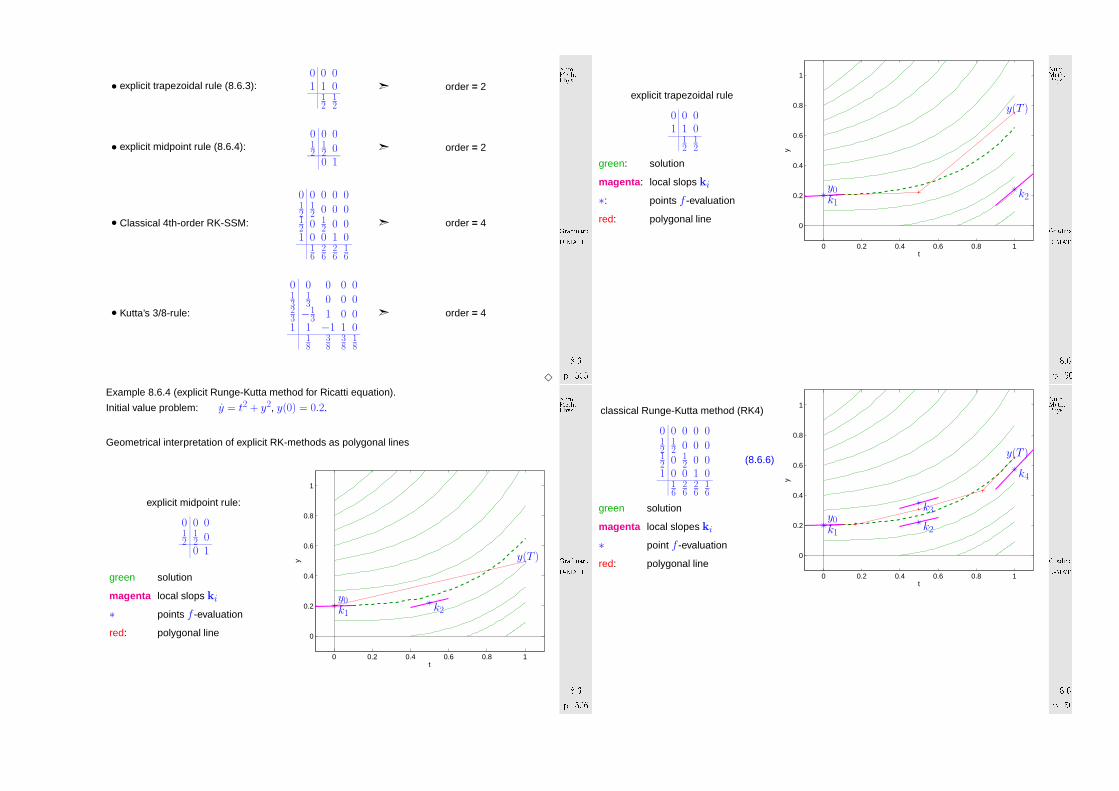
• explicit trapezoidal rule (8.6.3):0 0 01 1 0

12

12

order = 2

• explicit midpoint rule (8.6.4):0 0 012

12 00 1

order = 2

• Classical 4th-order RK-SSM:

0 0 0 0 012

12 0 0 0

12 0 1

2 0 01 0 0 1 0

16

26

26

16

order = 4

• Kutta’s 3/8-rule:

0 0 0 0 013

13 0 0 0

23 −1

3 1 0 01 1 −1 1 0

18

38

38

18

order = 4

3


Num.Meth.Phys.

Example 8.6.4 (explicit Runge-Kutta method for Ricatti equation).

Initial value problem: y = t2 + y2, y(0) = 0.2.

Geometrical interpretation of explicit RK-methods as polygonal lines

explicit midpoint rule:

0 0 012

12 00 1

green solution

magenta local slops ki

∗ points f -evaluation

red: polygonal line

0 0.2 0.4 0.6 0.8 1

0

0.2

0.4

0.6

0.8

1

t

y y(T )

y0k1

k2


Num.Meth.Phys.

explicit trapezoidal rule

0 0 01 1 0

12

12

green: solution

magenta: local slops ki

∗: points f -evaluation

red: polygonal line

0 0.2 0.4 0.6 0.8 1

0

0.2

0.4

0.6

0.8

1

t

y

y(T )

y0k1

k2


Num.Meth.Phys.

classical Runge-Kutta method (RK4)

0 0 0 0 012

12 0 0 0

12 0 1

2 0 01 0 0 1 0

16

26

26

16

(8.6.6)

green solution

magenta local slopes ki

∗ point f -evaluation

red: polygonal line0 0.2 0.4 0.6 0.8 1

0

0.2

0.4

0.6

0.8

1

t

y

y(T )

y0k1

k2

k3

k4


Num.Meth.Phys.

Kuttas 3/8-rule

0 0 0 0 013

13 0 0 0

23 −1

3 1 0 01 1 −1 1 0

18

38

38

18

(8.6.7)

green solution

magenta local slopes ki

∗ point f -evaluation

red: polygonal line0 0.2 0.4 0.6 0.8 1

0

0.2

0.4

0.6

0.8

1

t

y

y(T )

y0k1 k2

k3

k4

3

Remark 8.6.5 (“Butcher barriers” for explicit RK-SSM).

order p 1 2 3 4 5 6 7 8 ≥ 9minimal no.s of stages 1 2 3 4 6 7 9 11 ≥ p + 3

No general formula available so far

Known: order p < number s of stages of RK-SSM


Num.Meth.Phys.

Remark 8.6.6 (Explicit ODE integrator a la MATLAB).

Syntax:

t,y = ode45(odefun,tspan,y0);

odefun : Handle to a function of type (t,y)↔ r.h.s. f(t,y)

tspan : vector (t0, T )T , initial and final time for numerical integration

y0 : (vector) passing initial state y0 ∈ Rd

Return values:

t : temporal mesh t0 < t1 < t2 < · · · < tN−1 = tN = Ty : sequence (yk)Nk=0 (column vectors)


Num.Meth.Phys.

Example 8.6.7 (Numerical integration of logistic ODE ).

usage of ode45

from ode45 import ode45fn = lambda t, y: 5.*y*(1.-y)t,y = ode45(fn,(0, 1.5),[1.5])

integrator: ode45():

Handle passing r.h.s.

initial and final time

initial state y0

3

8.7 Stepsize control

Example 8.7.1 (Oregonator reaction).

Special case of oscillating Zhabotinski-Belousov reaction [21]:

BrO−3 + Br− 7→ HBrO2HBrO2 + Br− 7→ Org

BrO−3 + HBrO2 7→ 2 HBrO2 + Ce(IV)2 HBrO2 7→ Org

Ce(IV) 7→ Br−

(8.7.1)


Num.Meth.Phys.

y1 := c(BrO−3 ): y1 = −k1y1y2 − k3y1y3 ,y2 := c(Br−): y2 = −k1y1y2 − k2y2y3 + k5y5 ,y3 := c(HBrO2): y3 = k1y1y2 − k2y2y3 + k3y1y3 − 2k4y

23 ,

y4 := c(Org): y4 = k2y2y3 + k4y23 ,

y5 := c(Ce(IV)): y5 = k3y1y3 − k5y5 ,

(8.7.2)

with (non-dimensionalized) reaction constants:

k1 = 1.34 , k2 = 1.6 · 109 , k3 = 8.0 · 103 , k4 = 4.0 · 107 , k5 = 1.0 .

periodic chemical reaction Video 1, Video 2

simulation with inital state y1(0) = 0.06, y2(0) = 0.33 · 10−6, y3(0) = 0.501 · 10−10, y4(0) = 0.03,

y5(0) = 0.24 · 10−7:


Num.Meth.Phys.

0 20 40 60 80 100 120 140 160 180 20010

−10

10−9

10−8

10−7

10−6

10−5

10−4

10−3

Concentration of Br−

t

c(t)

Fig. 1230 20 40 60 80 100 120 140 160 180 200

10−11

10−10

10−9

10−8

10−7

10−6

10−5

t

c(t)

Concentration of HBrO2

Fig. 124

We observe a strongly non-uniform behavior of the solution in time.

This is very common with evolutions arising from practical models (circuit models, chemical reaction

models, mechanical systems)


Num.Meth.Phys.

3

Example 8.7.2 (Blow-up).

Scalar autonomous IVP:

y = y2 , y(0) = y0 > 0 .

y(t) =y0

1− y0t, t < 1/y0 .

Solution exists only for finite time and then suffers

a Blow-up, that is, limt→1/y0

y(t) = ∞ : J(y0) =

]−∞, 1/y0]!−1 −0.5 0 0.5 1 1.5 2 2.50

10

20

30

40

50

60

70

80

90

100

t

y(t

)

y

0 = 1

y0 = 0.5

y0 = 2

Fig. 125

How to choose temporal mesh t0 < t1 < · · · < tN−1 < tN for single step method in case J(y0)

is not known, even worse, if it is not clear a priori that a blow up will happen?

Just imagine: what will result from equidistant explicit Euler integration (8.2.1) applied to the above

IVP?


Num.Meth.Phys.

−1 −0.5 0 0.5 1 1.5 2 2.50

10

20

30

40

50

60

70

80

90

100

t

yk

solution by ode45

y

0 = 1

y0 = 0.5

y0 = 2

Fig. 126

1 odefun = lambda t , y : y∗∗2.02 p r i n t ’ y0 = ’ ,0 .53 t2 , y2 = ode45 ( odefun , ( 0 ,2 ) , 0 .5 ,

s t a t s =True )4 p r i n t ’ \ n ’ , ’ y0 = ’ ,15 t1 , y1 = ode45 ( odefun , ( 0 ,2 ) , 1 ,

s t a t s =True )6 p r i n t ’ \ n ’ , ’ y0 = ’ ,27 t3 , y3 = ode45 ( odefun , ( 0 ,2 ) , 2 ,

s t a t s =True )

warning messages:

y0 = 0.5error: OdePkg:InvalidArgumentSolving has not been successful. The iterative integration loop exited at time t = 2.00

Number of successful steps: 151Number of failed attempts: 74Number of function calls: 1344

y0 = 1error: OdePkg:InvalidArgumentSolving has not been successful. The iterative integration loop exited at time t = 1.00


Num.Meth.Phys.


y0 = 2error: OdePkg:InvalidArgumentSolving has not been successful. The iterative integration loop exited at time t = 0.50


We observe: ode45 manages to reduce stepsize more and more as it approaches the singularity of

the solution!

3

Key issue (discussed for autonomous ODEs below):

Choice of good temporal mesh 0 = t0 < t1 < · · · < tN−1 < tNfor a given single step method applied to an IVP

What does “good” mean ?


Num.Meth.Phys.

be efficient be accurate'

&

$

%

Objective: N as small as possible &max

k=1,...,N‖y(tk)− yk‖<TOL

or ‖y(T )− yN‖ < TOL

, TOL = tolerance

Policy: Try to curb/balance one-step error by

adjusting current stepsize hk,

predicting suitable next timestep hk+1

local-in-time

stepsize control

Tool: Local-in-time one-step error estimator (a posteriori, based on yk, hk−1)

Why local-in-time timestep control (based on estimating the one-step error)?

Consideration: If a small time-local error in a single timestep leads to large error ‖yk − y(tk)‖ atlater times, then local-in-time timestep control is powerless about it and will not even notice!!

Nevertheless, local-in-time timestep control is used almost exclusively,

because we do not want to discard past timesteps, which could amount to tremendous waste ofcomputational resources,


Num.Meth.Phys.

because it is inexpensive and it works for many practical problems,

because there is not reliable method that can deliver guaranteed accuracy for general IVP.

“Recycle” heuristics already employed for adaptive quadrature, see Sect. 7.3:

Idea: Estimation of one-step error, cf. Sect. 7.3

Compare two discrete evolutions Ψh, Ψh

of different order

for current timestep h:

If Order(Ψ) > Order(Ψ)

⇒ Φhy(tk)−Ψhy(tk)︸︷︷︸one-step error

≈ ESTk := Ψhy(tk)−Ψhy(tk) . (8.7.3)

Heuristics for concrete h

absolute tolerance

CompareESTk ↔ ATOL

ESTk ↔ RTOL ‖yk‖ Reject/accept current step (8.7.4)

relative tolerance


Num.Meth.Phys.

Simple algorithm:

ESTk < maxATOL, ‖yk‖ RTOL: Carry out next timestep (stepsize h)

Use larger stepsize (e.g., αh with some α > 1) for following step

(∗)ESTk > maxATOL, ‖yk‖ RTOL: Repeat current step with smaller stepsize < h, e.g., 1

2h

Rationale for (∗): if the current stepsize guarantees sufficiently small one-step error, then it might

be possible to obtain a still acceptable one-step error with a larger timestep, which would enhance

efficiency (fewer timesteps for total numerical integration). This should be tried, since timestep control

will usually provide a safeguard against undue loss of accuracy.

Code 8.7.3: simple local stepsize control for single step methods1 def odein tadapt ( Psi low , Psih igh , T , y0 , h0 , r e l t o l , abs to l , hmin ) :2 t = [ 0 ] ; y =[ y0 ] ; h=h0 #3 w h il e t [−1] < T and h > hmin :4 yh = Ps ih igh ( h , y0 )5 yH = Psi low ( h , y0 )6 est = norm (yH−yh )7 i f est < max( r e l t o l ∗norm ( y0 ) , abs to l ) :8 y0 = yh ; y . append ( y0 ) ;

t . append ( t [−1]+min (T−t [−1] ,h ) )9 h = 1.1∗h


Num.Meth.Phys.

10 el se :11 h = h / 2 . 012 r et u r n ( a r ray ( t ) , a r ray ( y ) )13

14 def ode in tadapt_ex t ( Psi low , Psih igh , T , y0 , h0 , r e l t o l , abs to l , hmin ) :15 " " " extended vers ion o f ode in tadapt . a lso r e tu r n s vec to r o f

r e j e c te d po in ts and vec to r o f est imated e r r o r s " " "16 t = [ 0 ] ; y =[ y0 ] ; h=h0 ; r e j = [ ] ; ee = [ 0 ]17 w h il e t [−1] < T and h > hmin :18 yh = Ps ih igh ( h , y0 )19 yH = Psi low ( h , y0 )20 est = norm (yH−yh )21 i f est < max( r e l t o l ∗norm ( y0 ) , abs to l ) :22 # print ’accept step, h = y0 = yh; y.append(y0); t.append(t[-1]+min(T-t[-1],h))23 h = 1.1∗h ; ee . append ( es t )24 el se :25 # print ’reject step, h = rej = hstack([rej,t]); h = h/2.026 r et u r n ( a r ray ( t ) , a r ray ( y ) , r e j , ee )

Comments on Code 8.7.2:

• Input arguments:


Num.Meth.Phys.

– Psilow, Psihigh: function handles to discrete evolution operators for autonomous ODE of

different order, type @(y,h), expecting a state (column) vector as first argument, and a

stepsize as second,

– T: final time T > 0,

– y0: initial state y0,

– h0: stepsize h0 for the first timestep

– reltol, abstol: relative and absolute tolerances, see (8.7.4),

– hmin: minimal stepsize, timestepping terminates when stepsize control hk < hmin, which is

relevant for detecting blow-ups or collapse of the solution.

• line ?? : check whether final time is reached or timestepping has ground to a halt (hk < hmin).

• line ?? , ?? : advance state by low and high order integrator.

• line ?? : compute norm of estimated error, see (?? ).

• line ?? : make comparison (8.7.4) to decide whether to accept or reject local step.

• line ?? , ?? : step accepted, update state and current time and suggest 1.1 times the current

stepsize for next step.

• line ?? step rejected, try again with half the stepsize.

• Return values:


Num.Meth.Phys.

– t: temporal mesh t0 < t1 < t2 < . . . < tN < T , where tN < T indicated premature

termination (collapse, blow-up),

– y: sequence (yk)Nk=0.

!By the heuristic considerations, see (8.7.3) it seems that ESTk measures the one-step error for

the low-order method Ψ and that we should use yk+1 = Ψhkyk, if the timestep is accepted.

However, it would be foolish not to use the better value yk+1 = Ψhk

yk, since it is available for free.

This is what is done in every implementation of adaptive methods, also in Code 8.7.2, and this choice

can be justified by control theoretic arguments [13, Sect. 5.2].

Example 8.7.4 (Simple adaptive stepsize control).

IVP for ODE y = cos(αy)2, α > 0, solution y(t) = arctan(α(t− c))/α for y(0) ∈]−π/2, π/2[

Simple adaptive timestepping based on explicit Euler (8.2.1) and explicit trapezoidal rule (8.6.3)

Code 8.7.5: function for Ex. 8.7.41 def o d e i n ta d a p td r i ve r (T , a , r e l t o l =1e−2, abs to l =1e−4) :


Num.Meth.Phys.

2 " " " Simple adapt ive t imestepp ing s t r a te g y o fCode~\ r e f mc: ode in tadapt

3 based on e x p l i c i t Eu ler \ eqre f eq : eeul and e x p l i c i tt r a p e z o i d a l

4 r u l e \ eqre f eq : exTrap 5 " " "6

7 # autonomous ODE y = cos(ay) and its general solution8 f = lambda y : ( cos ( a∗y ) ∗∗2)9 so l = lambda t : a rc tan ( a∗( t−1) ) / a

10 # Initial state y011 y0 = so l ( 0 )12

13 # Discrete evolution operators, see Def. 8.2.114 # Explicit Euler (8.2.1)15 Psi low = lambda h , y : y + h∗ f ( y )16 # Explicit trapzoidal rule (8.6.3)17 Psih igh = lambda h , y : y + 0.5∗h∗( f ( y ) + f ( y+h∗ f ( y ) ) )18

19 # Heuristic choice of initial timestep and hmin20 h0 = T / ( 1 0 0 .0∗ ( norm ( f ( y0 ) ) +0 .1) ) ; hmin = h0 /10000 .0 ;21 # Main adaptive timestepping loop, see Code 8.7.222 t , y , r e j , ee =


Num.Meth.Phys.

ode in tadapt_ex t ( Psi low , Psih igh , T , y0 , h0 , r e l t o l , abs to l , hmin )23

24 # Plotting the exact the approximate solutions and rejected timesteps25 f i g = p l t . f i g u r e ( )26 tp = r_ [ 0 : T : T /1000 .0 ]27 p l t . p l o t ( tp , so l ( tp ) , ’ g− ’ , l i n e w i d t h =2 , l a b e l= r ’y(t) ’ )28 p l t . p l o t ( t , y , ’ r . ’ , l a b e l= r ’yk ’ )29 p l t . p l o t ( r e j , zeros ( len ( r e j ) ) , ’m+ ’ , l a b e l= ’ r e j e c t i o n ’ )30 p l t . t i t l e ( ’ Adapt ive t imestepp ing , r t o l = %1.2 f , a t o l = %1.4 f , a

= %d ’ % ( r e l t o l , abs to l , a ) )31 p l t . x l a b e l ( r ’t ’ , f o n t s i z e =14)32 p l t . y l a b e l ( r ’y ’ , f o n t s i z e =14)33 p l t . legend ( loc= ’ upper l e f t ’ )34 p l t . show ( )35 # plt.savefig(’../PICTURES/odeintadaptsol.eps’)36

37 p r i n t ’%d t imesteps , %d r e j e c te d t imesteps ’ %( s ize ( t )−1, len ( r e j ) )

38

39 # Plotting estimated and true errors40 f i g = p l t . f i g u r e ( )41 p l t . p l o t ( t , abs ( so l ( t ) − y ) , ’ r + ’ , l a b e l= r ’ t r u e e r r o r |y(tk)− yk| ’ )42 p l t . p l o t ( t , ee , ’m∗ ’ , l a b e l= ’ est imated e r r o r EST_k ’ )


Num.Meth.Phys.

43 p l t . x l a b e l ( r ’t ’ , f o n t s i z e =14)44 p l t . y l a b e l ( r ’error ’ , f o n t s i z e =14)45 p l t . legend ( loc= ’ upper l e f t ’ )46 p l t . t i t l e ( ’ Adapt ive t imestepp ing , r t o l = %1.2 f , a t o l = %1.4 f , a

= %d ’ % ( r e l t o l , abs to l , a ) )47 p l t . show ( )48 # plt.savefig(’../PICTURES/odeintadapterr.eps’)49

50 i f __name__ == ’ __main__ ’ :51 o d e i n ta d a p td r i ve r (T=2 ,a=20 , r e l t o l =1e−2, abs to l =1e−4)


Num.Meth.Phys.0 0.2 0.4 0.6 0.8 1 1.2 1.4 1.6 1.8 2

−0.08

−0.06

−0.04

−0.02

0

0.02

0.04

0.06

0.08Adaptive timestepping, rtol = 0.010000, atol = 0.000100, a = 20.000000

t

y

y(t)y

k

rejection

Fig. 1270 0.2 0.4 0.6 0.8 1 1.2 1.4 1.6 1.8 2

0

0.005

0.01

0.015

0.02

0.025

t

err

or

Adaptive timestepping, rtol = 0.010000, atol = 0.000100, a = 20.000000

true error |y(t

k)−y

k|

estimated error ESTk

Fig. 128

Statistics: 66 timesteps, 131 rejected timesteps

Observations:

Adaptive timestepping well resolves local features of solution y(t) at t = 1

Estimated error (an estimate for the one-step error) and true error are not related!

3


Num.Meth.Phys.

Example 8.7.6 (Gain through adaptivity). → Ex. 8.7.4

Simple adaptive timestepping from previous experiment Ex. 8.7.4.

New: initial state y(0) = 0!

Now we study the dependence of the maximal point error on the computational effort, which is pro-

portional to the number of timesteps.

0 0.2 0.4 0.6 0.8 1 1.2 1.4 1.6 1.8 20

0.005

0.01

0.015

0.02

0.025

0.03

0.035

0.04

0.045

0.05

t

y

Solving dt y = a cos(y)2 with a = 40.000000 by simple adaptive timestepping

rtol = 0.400000rtol = 0.200000rtol = 0.100000rtol = 0.050000rtol = 0.025000rtol = 0.012500rtol = 0.006250

Fig. 129

Solutions (yk)k for different values of rtol

101

102

103

10−5

10−4

10−3

10−2

10−1

100

101

no. N of timesteps

max

k|y(t

k)−y k|

Error vs. no. of timesteps for dt y = a cos(y)2 with a = 40.000000

uniform timestepadaptive timestep

Fig. 130

Error vs. computational effort


Num.Meth.Phys.

Observations:

Adaptive timestepping achieves much better accuracy for a fixed computational effort.

3

Example 8.7.7 (“Failure” of adaptive timestepping). → Ex. 8.7.6

Same ODE and simple adaptive timestepping as in previous experiment Ex. 8.7.6. Same evaluations.

Now: initial state y(0) = −0.0386 as in Ex. 8.7.4


Num.Meth.Phys.

0 0.2 0.4 0.6 0.8 1 1.2 1.4 1.6 1.8 2−0.05

−0.04

−0.03

−0.02

−0.01

0

0.01

0.02

0.03

0.04

0.05

t

y

Solving dt y = a cos(y)2 with a = 40.000000 by simple adaptive timestepping

rtol = 0.400000rtol = 0.200000rtol = 0.100000rtol = 0.050000rtol = 0.025000rtol = 0.012500rtol = 0.006250

Fig. 131

Solutions (yk)k for different values of rtol

101

102

103

10−3

10−2

10−1

100

no. N of timesteps

max

k|y(t

k)−y k|

Error vs. no. of timesteps for dt y = a cos(y)2 with a = 40.000000

uniform timestepadaptive timestep

Fig. 132

Error vs. computational effort

Observations:

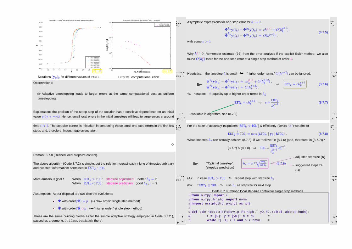
Adaptive timestepping leads to larger errors at the same computational cost as uniform

timestepping.

Explanation: the position of the steep step of the solution has a sensitive dependence on an initial

value y(0) ≈ −π/2. Hence, small local errors in the initial timesteps will lead to large errors at around


Num.Meth.Phys.

time t ≈ 1. The stepsize control is mistaken in condoning these small one-step errors in the first few

steps and, therefore, incurs huge errors later.

3

Remark 8.7.8 (Refined local stepsize control).

The above algorithm (Code 8.7.2) is simple, but the rule for increasing/shrinking of timestep arbitraryand “wastes” informatiom contained in ESTk : TOL:

More ambitious goal ! When ESTk > TOL : stepsize adjustment better hk = ?When ESTk < TOL : stepsize prediction good hk+1 = ?

Assumption: At our disposal are two discrete evolutions:

Ψ with order(Ψ) = p ( “low order” single step method)

Ψ with order(Ψ)>p ( “higher order” single step method)

These are the same building blocks as for the simple adaptive strategy employed in Code 8.7.2 (,passed as arguments Psilow, Psihigh there).


Num.Meth.Phys.

Asymptotic expressions for one-step error for h→ 0:

Ψhky(tk)−Φhky(tk) = chp+1 + O(hp+2k ) ,

Ψhk

y(tk)−Φhky(tk) = O(hp+2) ,(8.7.5)

with some c > 0.

Why hp+1? Remember estimate (?? ) from the error analysis if the explicit Euler method: we also

found O(h2k) there for the one-step error of a single step method of order 1.

Heuristics: the timestep h is small “higher order terms” O(hp+2) can be ignored.

Ψhky(tk)−Φhky(tk).= ch

p+1k + O(h

p+2k ) ,

Ψhk

y(tk)−Φhky(tk).= O(h

p+2k ) .

⇒ ESTk.= ch

p+1k . (8.7.6)

notation:.= equality up to higher order terms in hk

ESTk.= ch

p+1k ⇒ c

.=

ESTk

hp+1k

. (8.7.7)

Available in algorithm, see (8.7.3)


Num.Meth.Phys.

For the sake of accuracy (stipulates “ESTk < TOL”) & efficiency (favors “>”) we aim for

ESTk!= TOL := maxATOL, ‖yk‖ RTOL . (8.7.8)

What timestep h∗ can actually achieve (8.7.8), if we “believe” in (8.7.6) (and, therefore, in (8.7.7))?

(8.7.7) & (8.7.8) ⇒ TOL =ESTk

hp+1k

hp+1∗ .

"‘Optimal timestep”:(stepsize prediction)

h∗ = h p+1

√TOL

ESTk. (8.7.9)

adjusted stepsize (A)

suggested stepsize

(B)

(A): In case ESTk > TOL repeat step with stepsize h∗.

(B): If ESTk ≤ TOL use h∗ as stepsize for next step.

Code 8.7.9: refined local stepsize control for single step methods1 from numpy impo r t ∗2 from numpy . l i n a l g impo r t norm3 impo r t m a t p l o t l i b . pyp lo t as p l t4

5 def o d e i n t s s c t r l ( Psi low , p , Psih igh , T , y0 , h0 , r e l t o l , abs to l , hmin ) :6 t = [ 0 ] ; y = [ y0 ] ; h = h0 #7 w h il e t [−1] < T and h > hmin : #


Num.Meth.Phys.

8 yh = Ps ih igh ( h , y0 ) #9 yH = Psi low ( h , y0 ) #

10 est = norm (yH−yh ) #11 t o l = max( r e l t o l ∗norm ( y [−1]) , abs to l ) #12 h = h∗max( 0 . 5 , min ( 2 , ( t o l / es t ) ∗∗ ( 1 . 0 / ( p+1) ) ) ) #13 i f est < t o l : #14 y0 = yh ; y . append ( y0 ) ;

t . append ( t [−1]+min (T−t [−1] ,h ) ) #15

16 r et u r n ( a r ray ( t ) , a r ray ( y ) ) # convert to numpy array17

18 i f __name__ == ’ __main__ ’ :19 " " " t h i s example demonstrates t h a t a s l i g h t reduc t i on i n the20 t o l e rance can have a la rge e f f e c t on the q u a l i t y o f the

s o l u t i o n21 " " "22 # use two different tolerances23 r e l t o l 1 =1e−2; abs to l1=1e−424 r e l t o l 2 =1e−3; abs to l2=1e−525 T=2; a=2026

27 # autonomous ODE y = cos(ay) and its general solution28 f = lambda y : ( cos ( a∗y ) ∗∗2)


Num.Meth.Phys.

29 so l = lambda t : a rc tan ( a∗( t−1) ) / a30 # Initial state y031 y0 = so l ( 0 )32

33 # Discrete evolution operators, see Def. 8.2.134 Psi low = lambda h , y : y + h∗ f ( y ) # Explicit Euler (8.2.1)35 o = 1 # global order of lower-order evolution36 Psih igh = lambda h , y : y + 0.5∗h∗( f ( y ) + f ( y+h∗ f ( y ) ) ) # Explicit

trapzoidal rule (8.6.3)37

38 # Heuristic choice of initial timestep and hmin39 h0 = T / ( 1 0 0 .0∗ ( norm ( f ( y0 ) ) +0 .1) ) ; hmin = h0 /10000 .0 ;40 # Main adaptive timestepping loop, see Code 8.7.241 t1 , y1 =

o d e i n t s s c t r l ( Psi low , o , Psih igh , T , y0 , h0 , r e l t o l 1 , absto l1 , hmin )42 t2 , y2 =

o d e i n t s s c t r l ( Psi low , o , Psih igh , T , y0 , h0 , r e l t o l 2 , absto l2 , hmin )43

44 # Plotting the exact the approximate solutions and rejected timesteps45 f i g = p l t . f i g u r e ( )46 tp = r_ [ 0 : T : T /1000 .0 ]47 p l t . p l o t ( tp , so l ( tp ) , ’ g− ’ , l i n e w i d t h =2 , l a b e l= r ’y(t) ’ )48 p l t . p l o t ( t1 , y1 , ’ r . ’ , l a b e l= ’ r e l t o l : %1.3 f , abs to l :

%1.5 f ’%( r e l t o l 1 , abs to l1 ) )


Num.Meth.Phys.

49 p l t . p l o t ( t2 , y2 , ’ b . ’ , l a b e l= ’ r e l t o l : %1.3 f , abs to l :%1.5 f ’%( r e l t o l 2 , abs to l2 ) )

50 p l t . t i t l e ( ’ Adapt ive t imestepp ing , a = %d ’ % a )51 p l t . x l a b e l ( r ’t ’ , f o n t s i z e =14)52 p l t . y l a b e l ( r ’y ’ , f o n t s i z e =14)53 p l t . legend ( loc= ’ upper l e f t ’ )54 p l t . show ( )55 # plt.savefig(’../PICTURES/odeintssctrl.eps’)

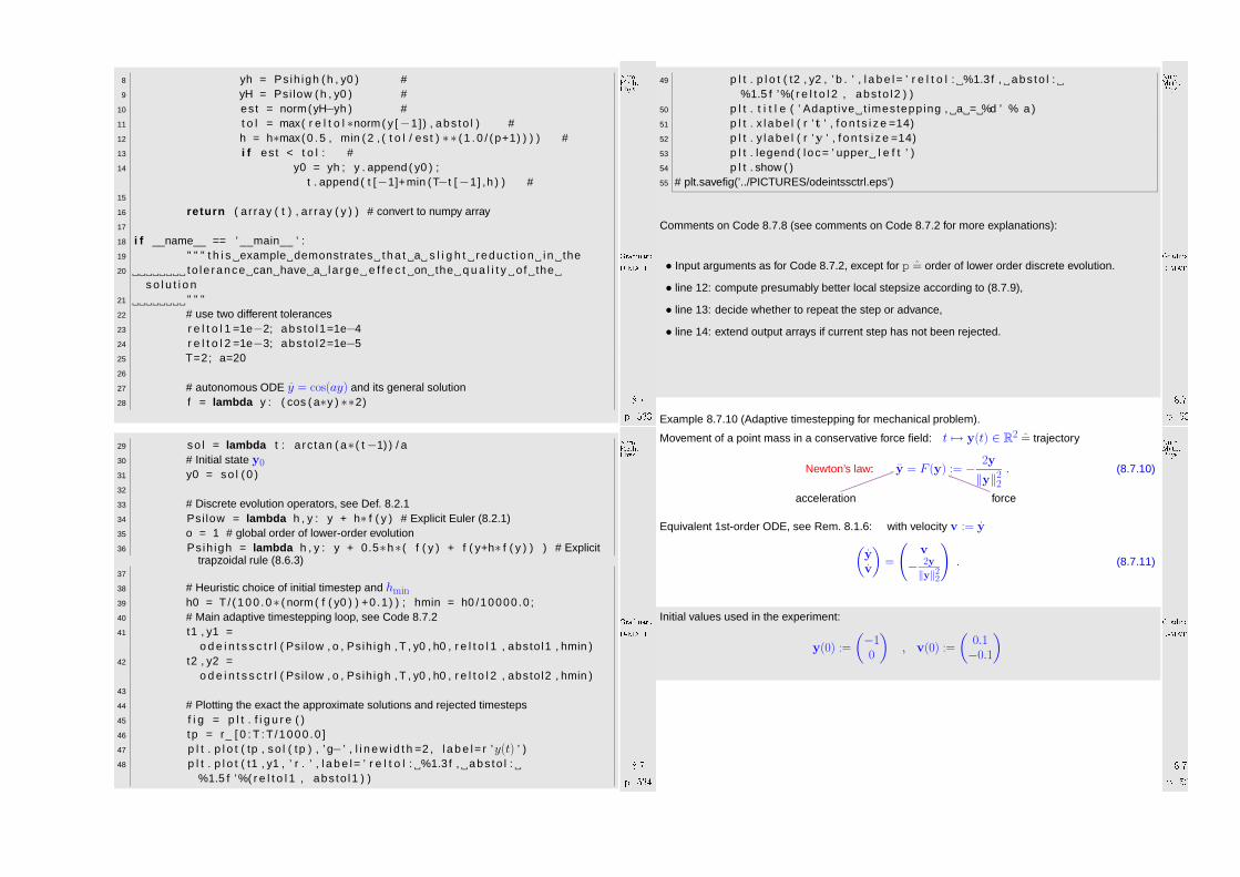
Comments on Code 8.7.8 (see comments on Code 8.7.2 for more explanations):

• Input arguments as for Code 8.7.2, except for p = order of lower order discrete evolution.

• line 12: compute presumably better local stepsize according to (8.7.9),

• line 13: decide whether to repeat the step or advance,

• line 14: extend output arrays if current step has not been rejected.

Example 8.7.10 (Adaptive timestepping for mechanical problem).


Num.Meth.Phys.

Movement of a point mass in a conservative force field: t 7→ y(t) ∈ R2 = trajectory

Newton’s law: y = F (y) := − 2y

‖y‖22. (8.7.10)

acceleration force

Equivalent 1st-order ODE, see Rem. 8.1.6: with velocity v := y

(y

v

)=

(v

− 2y

‖y‖22

). (8.7.11)

Initial values used in the experiment:

y(0) :=

(−10

), v(0) :=

(0.1−0.1

)


Num.Meth.Phys.

0 0.5 1 1.5 2 2.5 3 3.5 4−4

−3

−2

−1

0

1

2

3

4

t

abstol = 0.000010, reltol = 0.001000

y

1(t) (exakt)

y2(t) (exakt)

v1(t) (exakt)

v2(t) (exakt)

0 0.5 1 1.5 2 2.5 3 3.5 4−5

0

5

t

y i(t)

abstol = 0.000010, reltol = 0.001000

0 0.5 1 1.5 2 2.5 3 3.5 40

0.1

0.2

Zei

tsch

rittw

eite

y1(t

k) (Naeherung)

y2(t

k) (Naeherung)

v1(t

k) (Naeherung)

v2(t

k) (Naeherung)


Num.Meth.Phys.0 0.5 1 1.5 2 2.5 3 3.5 4

−4

−3

−2

−1

0

1

2

3

4

t

abstol = 0.001000, reltol = 0.010000

y

1(t) (exakt)

y2(t) (exakt)

v1(t) (exakt)

v2(t) (exakt)

0 0.5 1 1.5 2 2.5 3 3.5 4−5

0

5

t

y i(t)

abstol = 0.001000, reltol = 0.010000

0 0.5 1 1.5 2 2.5 3 3.5 40

0.1

0.2

Zei

tsch

rittw

eite

y1(t

k) (Naeherung)

y2(t

k) (Naeherung)

v1(t

k) (Naeherung)

v2(t

k) (Naeherung)


Num.Meth.Phys.

−1 −0.5 0 0.5 1−1

−0.8

−0.6

−0.4

−0.2

0

0.2

0.4

0.6

0.8

y1

y 2

Exakte BahnNaeherung

reltol=0.001, abstol=1e-5

−1 −0.5 0 0.5 1−1

−0.8

−0.6

−0.4

−0.2

0

0.2

0.4

0.6

0.8

y1

y 2

Exakte BahnNaeherung

reltol=0.01, abstol=1e-3

Observations:

Fast changes in solution components captured by adaptive approach through very small

timesteps.

Completely wrong solution, if tolerance reduced slightly.


Num.Meth.Phys.

3

An inevitable consequence of time-local error estimation:

Absolute/relative tolerances do not allow to predict accuracy of solution!

8.8 Essential Skill s Learned in Chapter 8

You should know:

• what is an autonomous ODE

• how to reduce an ODE to an autonomous first order system of ODEs

• the meaning of evolution operator

• the Euler methods with pros and contras

• the derivation and advantages of the implicit midpoint rule


Num.Meth.Phys.

Documents

Num. Meth. Ph 8 Single Step Methods A - D-MATH