NUM-NUM analysis student worksheet

© TexasInstruments2017.Youmaycopy,communicateandmodifythismaterialfornon-commercialeducationalpurposesprovidedallacknowledgementsassociatedwiththismaterialaremaintained.

Author:D.Tynan

NUM-NUM Analysis

Student Worksheet

TI-NspireCAS

Investigation

Student

90min789101112

NUM-NUM analysis Ifwehavedatafromtwonumericvariables(i.e.‘NUM–NUM’),wemaybeinterestedinthestatisticalrelationshipbetweenthem–itmaybeusefulasawayofpredictingvaluesoftheresponsevariable(y),fromthevaluesoftheexplanatoryvariable(x).

Fromyourpreviousstudyofbivariatedataanalysis,youmayrecallthefollowing:

• Produceascatterplot,andobservetheplot,andlookforevidenceofanassociationbetweenthevariables.

• Ifthescatterplotsuggestsanassociation,wemaylookatPearson’scorrelationcoefficient(r)orthecoefficientofdetermination(r2)toconfirmourobservation.

• Ifthesevaluesarestrongenough,wemaytrytofitalineoftheformy = a+bx ,andperhapsusethistohelppredictothervaluesofyfromgivenxvalues.

InYear12FurtherMathematics,welookatsomenewwaysofevaluatingwhetheralinearmodelisappropriate.

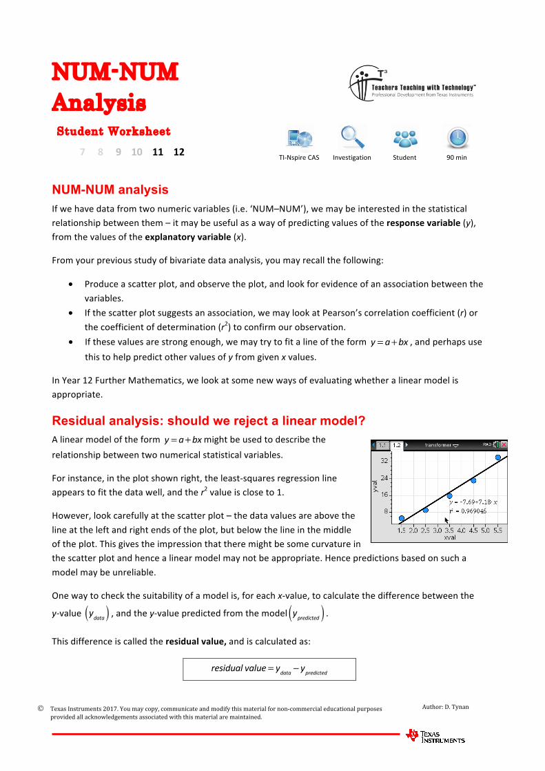
Residual analysis: should we reject a linear model? Alinearmodeloftheformy = a+bxmightbeusedtodescribetherelationshipbetweentwonumericalstatisticalvariables.

Forinstance,intheplotshownright,theleast-squaresregressionlineappearstofitthedatawell,andther2valueiscloseto1.

However,lookcarefullyatthescatterplot–thedatavaluesareabovethelineattheleftandrightendsoftheplot,butbelowthelineinthemiddleoftheplot.Thisgivestheimpressionthattheremightbesomecurvatureinthescatterplotandhencealinearmodelmaynotbeappropriate.Hencepredictionsbasedonsuchamodelmaybeunreliable.

Onewaytocheckthesuitabilityofamodelis,foreachx-value,tocalculatethedifferencebetweenthe

y-valueydata( ) ,andthey-valuepredictedfromthemodel

ypredicted( ) .

Thisdifferenceiscalledtheresidualvalue,andiscalculatedas:

residual value = ydata − ypredicted


Author:D.Tynan

2 NUM–NUMAnalysis–StudentWorksheet

Aresidualplotisaplotoftheseresidualvalues(againsteachxvalue).Forexampletheresidualplot(underneaththescatterplot)highlightswhethertheregressionruleoverpredictsorunderpredictsforeachx-value,andbyhowmuch.Forexample,itshowsthatthedatapoint(4.5,23.1)onthescatterplothasaresidualvalueof–1.520,whichmeansthatthepredictedy-valueis1.520unitshigherthantheactualdatay-value(i.e.themodeloverpredictsthatvalueofy).

Further,ifalinearmodelwasappropriate,theresidualvalueswouldberandomlypositionedaroundzero.Sothecurvatureintheresidualplotsuggestsalinearmodeldoesnotexplaintherelationshipwell.

Choosing a non-linear model Ifitisclearfromaresidualplotthatalinearmodel(i.e.y = a+bx )isnotsuitable,itispossiblethatanon-

linearmodel(forexampley = a+bx2 )maybesuitable.

Tohelpdecide,weconsiderwhetherachange(transformation)toeithertheexplanatoryvariable(x),ortheresponsevariable(y)resultsinabettermodel.

ThepossibletransformationsweconsiderinYear12FurtherMathematicsare:

Transformationsofthex-variable Transformationsofthey-variable

y = a+bx2 y

2 = a+bx

y = a+blog10(x) log10(y)= a+bx

y = a+ b

x

1y= a+bx

Inevaluatingthesuitabilityofaparticulartransformation,weneedtoconsiderwhathappensasaresultofthetransformation:

• doesthetransformation‘straighten’thescatterplot(makeitmore‘line–like’)?• dothenewresidualvaluesappeartoberelativelysmallandrandomlyscatteredaroundzero• Isthecoefficientofdeterminationimproved(i.e.isr2closerto1?)

The circle of transformations Thediagramatrightisveryhelpfulinnarrowingthechoiceofsuitablenon-linearmodels.Checkthecurvatureoftheoriginalplot.Forexample,thescatterplotconsideredearliersuggestsoneofthefollowingthreetransformationsmaybesuitable.

• A‘log-y’transformation(model:log10(y)= a+bx )

• A‘1/y’transformation(model:

1y= a+bx )

• An‘x2’transformation(model:y = a+bx2 )

OKsowhatnext?WewillbuildaTI-Nspiretemplatefilecalled‘transformer’,whichmakesitmucheasiertodecidewhichmodel(linearornon-linearmodel)isappropriate.


Author:D.Tynan


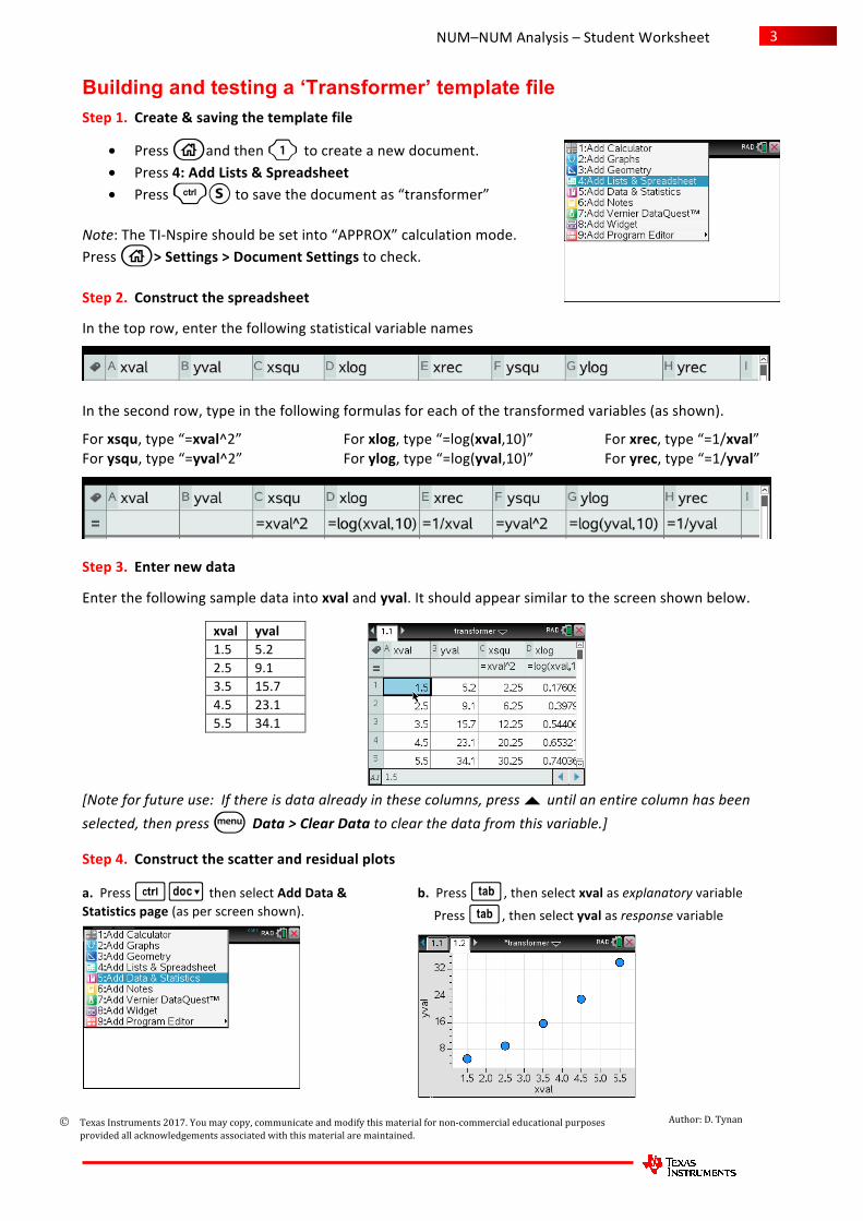
Building and testing a ‘Transformer’ template file Step1. Create&savingthetemplatefile

• Presscandthen1 tocreateanewdocument.• Press4:AddLists&Spreadsheet• Press/Stosavethedocumentas“transformer”

Note:TheTI-Nspireshouldbesetinto“APPROX”calculationmode.Pressc>Settings>DocumentSettingstocheck.Step2. Constructthespreadsheet

Inthetoprow,enterthefollowingstatisticalvariablenames

Inthesecondrow,typeinthefollowingformulasforeachofthetransformedvariables(asshown).

Forxsqu,type“=xval^2” Forxlog,type“=log(xval,10)” Forxrec,type“=1/xval”Forysqu,type“=yval^2” Forylog,type“=log(yval,10)” Foryrec,type“=1/yval”

Step3. Enternewdata

Enterthefollowingsampledataintoxvalandyval.Itshouldappearsimilartothescreenshownbelow.

xval yval

1.5 5.22.5 9.13.5 15.74.5 23.15.5 34.1

[Noteforfutureuse:Ifthereisdataalreadyinthesecolumns,press£ untilanentirecolumnhasbeenselected,thenpressb Data>ClearDatatoclearthedatafromthisvariable.]

Step4. Constructthescatterandresidualplots

a.Press/~thenselectAddData&Statisticspage(asperscreenshown).

b.Presse,thenselectxvalasexplanatoryvariable

Presse,thenselectyvalasresponsevariable


Author:D.Tynan


c.PressbAnalyse>Regression>ShowLinear(a+bx)

d.Thiswillbetheresultinglinewithequationshown

e.PressbAnalyse>Residuals>ShowResidualPlot

f.Thisplacestheresidualplotunderthescatterplot.

Step5. Transformvariablesandcheckthecoefficientofdeterminationg.Toperformatransformation,clickoneitherthexvaloryvalandchangeit.

h.Theplotsareupdated.[Note:Togetabetterviewoftheresiduals,pressb>Window/Zoom>Zoom–Data]

i.Pressb>Settingsandclick‘Diagnostics’sothatther2valuediagnosticisdisplayed.

j.Notethatther2valueisnowdisplayedundertheregressionequation.

k.Saveyourtemplatefileagainwith,anditisreadytouseforfutureanalyses!


Author:D.Tynan


What we just did … Asthe‘xsqu’(x-squared)transformationhasstraightenedthescatterplot,andtheresidualvaluesseemtobesmallandrandomlyscatteredaboutzero,wecansaythatan‘x-squared’modelisreasonable.

Thismeansthattheequationy = a+bx2 ormorespecificallyy =2.805+1.027x2 (correctto3decimal

places)isabettermodeltodescribetherelationship.Ther2value(0.999)isalsohigher,whichmeansthat99.9%ofthevariationintheresponsevariable(y)canbeexplainedbyvariationintheexplanatoryvariable(x).

A sample analysis … Thenumberofhoursspentdoinghomeworkeachweek(Homeworkhours)andthenumberofhoursspentwatchingtelevisioneachweek(TVhours)wererecordedforagroupof20Year12students.

TVhours 6 28 14 6 9 30 10 3 3 18 7 9 4 25 8 24 21 5 15 10Homeworkhours 17 16 9 21 17 8 15 48 37 9 21 18 24 14 14 10 14 32 6 13

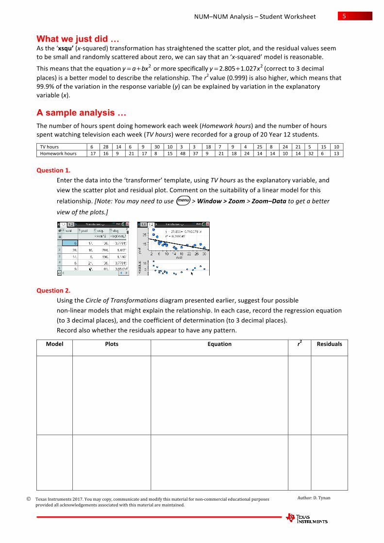
Question1. Enterthedataintothe‘transformer’template,usingTVhoursastheexplanatoryvariable,andviewthescatterplotandresidualplot.Commentonthesuitabilityofalinearmodelforthisrelationship.[Note:Youmayneedtouseb>Window>Zoom>Zoom–Datatogetabetterviewoftheplots.]

Thescatterplotlooksnon-linear,andthereisapatternintheresidualplot.Thecoefficientofdeterminationisalsolow,indicatingthat,forthelinearmodel,onlyabout40%ofthevariationinHomeworkhourscanbeexplainedbyvariationinTVhours.

Question2. UsingtheCircleofTransformationsdiagrampresentedearlier,suggestfourpossiblenon-linearmodelsthatmightexplaintherelationship.Ineachcase,recordtheregressionequation(to3decimalplaces),andthecoefficientofdetermination(to3decimalplaces).Recordalsowhethertheresidualsappeartohaveanypattern.

Model Plots Equation r2 Residuals

0.44 Patternevident

0.36 Patternevident


Author:D.Tynan


Model Plots Equation r2 Residuals

0.64 Patternevident

0.82 Nopatternevident

Question3. Onthebasisoftheseresults,proposethe‘best’ofthesefourmodels,givingreasons.

ThemostsuitabletransformationseemstobethereciprocalofTVhours,asitistheonlymodelthatappearstolinearisethescatterplot,andtheresidualplotappearstohavevaluesthatarerandomlyscatteredaboutzero.Thismodelalsohasthehighestcoefficientofdetermination.

Question4. Ifastudentspends10hoursperweekwatchingtelevision,useyourchosen‘best’model

topredictthenumberofhoursthatthestudentspendsdoinghomework.Giveyouranswercorrecttothenearesthour.Substituting12fortelevisionhoursintheequationgives

Documents

NUM-NUM analysis student worksheet