NUER WORKING PAPER SERIES

A BUPERGANE-TKEORflIC f'K)Dfl OFBUSINESS CYCLES ARD PRICE WARS

DURING BOOt.E

Julio 3. Rotemberg

Garth Saloner

Working Paper No. 12t12

NATIONAL BLThEAU OF !EONOMIC RESEARCH1050 Massachusetts Avenue

Cambridge, Mk 02138August 198b

Sloan School of Management and Department of Economics respectively.We are very grateful to James Poterba and Lawrence Sunners for manyhelpful conversations. Financial support from the National ScienceFoundation (grants SES—8209266 and SES—8308782 respectively) isgratefuL].y acknowledged. The research reported here is part of theNBER's research program in Economic Fluctuations. Any opinionsexpressed are those of the authors and not those of the NationalBureau of Economic Research.

NBER Working Paper #1412August 1984

A Supergame—Theoretic Model ofBusiness Cycles and Price Wars

During Booms

ABSTRACT

This paper studies implicitly colluding oligopolists facing fluctuating

demand. The credible threat of future punishments provides the discipline that

facilitates collusion. However, we find that the temptation to unilaterally

deflate from the collusive outcome is often greater when demand is high. To

moderate this temptation, the optimizing oligopoly reduces its profitability at

such times, resulting in lower prices. If the oligopolists' output is an inputto other sectors, their output may increase too. This explains the co—movements

of outputs which characterize business cycles. The behavior of the railroads in

the 1880's, the automobile industry in the 1950's and the cyclical behavior of

cement prices and price—cost margins support our theory. (J.E.L. Classification

nuzjzbers: 020, 130, 610).

Julio 3. Rotemberg Garth SalonerAlfred P. Sloan School Department of Economicsof Management, E52—250 E52—262B50 Memorial Drive M.I.T.M.I.T. Cambridge, MA 02139Cambridge, MA 02139

I. INTRODUCTION

This paper has two objectives. First it is an exploration of the

way in which oligopolies behave over the business cycle. Second, it

considers the possibility that this behaviour itself is a cause of

business cycles and of sticky prices. We examine implicitly colluding

cligopolies that attempt to sustain above competitive profits by the

threat of reverting to competitive behavior to punish firms that do not

cooperate. The basic point of the paper is that the oligopolists find

implicit collusion of this kind more difficult when their demand is high.

In other words when an industry faces a boom in its demand, chiseling

away from the collusive level of output becomes more profitable for each

individual firm and thus the oligopoly can only sustain a less collusive

outcome. This suggests that when demand for goods produced by

oligopolists is high, the economy produces an allocation which is

'closer" to the competitive allocation and thus nearer the production

possibility frontier. Insofar as the allocation in which the oligopoly

acts collusively is inside the production possibility frontier, a shift

in demand towards the oligopolistic sector can increase the output of all

goods. The fact that the outputs of all goods tend to move together is,

of course, the hallmark of business cycles. Thus we can interpret booms

in aggregate economic activity as being due to a shift in demand towards

the oligopolistic sectors and busts as shifts towards the competitive

sectors.

This analysis still leaves unexplained the causes of the shifts in

sectoral demands. To make sense of actual business cycles one would have

to relate these shifts in demand to changes in the money supply and

interest rates which are highly correlated with cyclical fluctuations.

2

tile the connection between financial variables and shifts in demand is

beyond the scope of this paper it must be noted that these shifts form

part of the popular discussions of the early stages of recoveries. At

that point consumers desire for cars and other durables usually picks

up.

The oligopolies we consider know that deviations from some agreed

upon strategy lead to punishments. Unfortunately there are usually a

multitude of equilibria in such settings. These equilibria differ in the

mechanics by which reversion to punishing behavior takes place, by the

length and intensity of the punishment interval as well as by the amount

of collusion that takes place when the firms are not punishing each

other. One standard technique for choosing among these equilibria (see,

for example, Porter (1983a)) is to concentrate on the equilibrium that is

optimal from the point of view of the oligopolists.

Unfortunately it is often very difficult to characterize these

optima. Even Porte?s paper considers only linear demand and optimizes

only over a subset of all the possible strategies. In particular, he

considers only punishments in which firms act as if they were involved in

a sequence of one—shot noncooperative games. Thus the most firms can do

to each other when they are punishing and being punished is to compete as

if they were playing a sequence of static games. This considerably

simplifies the analysis. Our otherwise optimal supergames also embody

this assumption which is not essential in all cases.

In our model the reversion to competitive behaviour occurs for a

period of infinite length. This length is optimal since it is the

biggest credible threat and since, along the equilibrium path, firma

never find themselves punishing each other. Instead for each state of

3

demand we focus on the outcome closest to monopoly that the oligopoly can

sustain given the threat. Any outcome closer to monopoly would lead to a

breakdown in discipline. Any outcome further from monopoly would simply

result in lower oligopoly profits. We show that when demand rises, the

best sustainable outcome generally becomes more competitive. Our

strongest results are for the case in which prices are the strategic

variable and there are constant marginal costs. Then an increase in

demand actually towers the oligopoly's prices monotonically after a

certain point. This occurs because keeping the oligopoly's price

constant when demand increases raises the payoff to a single firm from

towering its price slightly and thus capturing alt of demand. To deter

each firm from doing this the oligopoly must actually lower its price.

The paper proceeds as follows. Section II presents the optimal

supergame for both the cases in which the oligopoly treats prices and the

case in which it treats outputs as the strategic variable. Ye also

discuss simpler games in which, as in Breshnahan (1981), Green and Porter

(1964) and Porter (1983b) the oligopoly can only behave either

monopolistically or competitively. It is then in general more likely to

behave competitively when demand is high. Section III establishes the

connection with macroeconomics. It describes a simple two sector general

equilibrium model in which oRe sector is oligopolistic and the other

sector is competitive. The oligopolistic sector's output is purchased

both by consumers and by the competitive sector. When demand shifts

towards the oligopolistic sector, this sector lowers its prices. This,

in turn, leads the competitive sector to increase its purchases from the

oligopolistic sector and thus increase its output as well. So both

4

sectors grow, only to shrink when demand moves back towards the

competitive sector or when the punishment period is over.

Any theory whose foundation is that competitive behaviour is more

likely to occur in booms must confront the tact that the industrial

organization folklore is that price wars occur in recessions. This

folklore is articulated in Sherer (1980) for example. Our basis for

rejecting this folklore is not theoretical. We concede that tt is

possible to construct models in which recessions induce price wars.

Instead our rejection is based on facts. First, at a very general level,

it certainly appears that business cycles are related to sluggish

adjustment of prices (see Rotemberg (1982) for example). Prices rise too

little in booms and fall too little in recessions. If recessions tended

to produce massive price wars this would be an unlikely finding. !€ore

specifically we analyze some other sources of data capable of shedding

light on the folklore. That we find is that both Scherer's evidence and

our own study of the cyclical properties of price cost margins supports

our theory. Our theory is also supported by an analysis, of the price

wars purported to have happened in the automobile industry (Bresnahan

(1981)) and the railroad industry (Porter (1983a)). These wars have

occurred in periods of high demand. Finally, since Sherer singles out

the cenent industry as having repeated break—ups of its cartel during

recessions, we study the cyclical properties of cement prices. To our

surprise, cement prices are strongly countercyclical even though cement,

as construction as a whole, has a procyclical level of output. These

empirical regularities are discussed in Section IV. We conclude with

Section V.

5

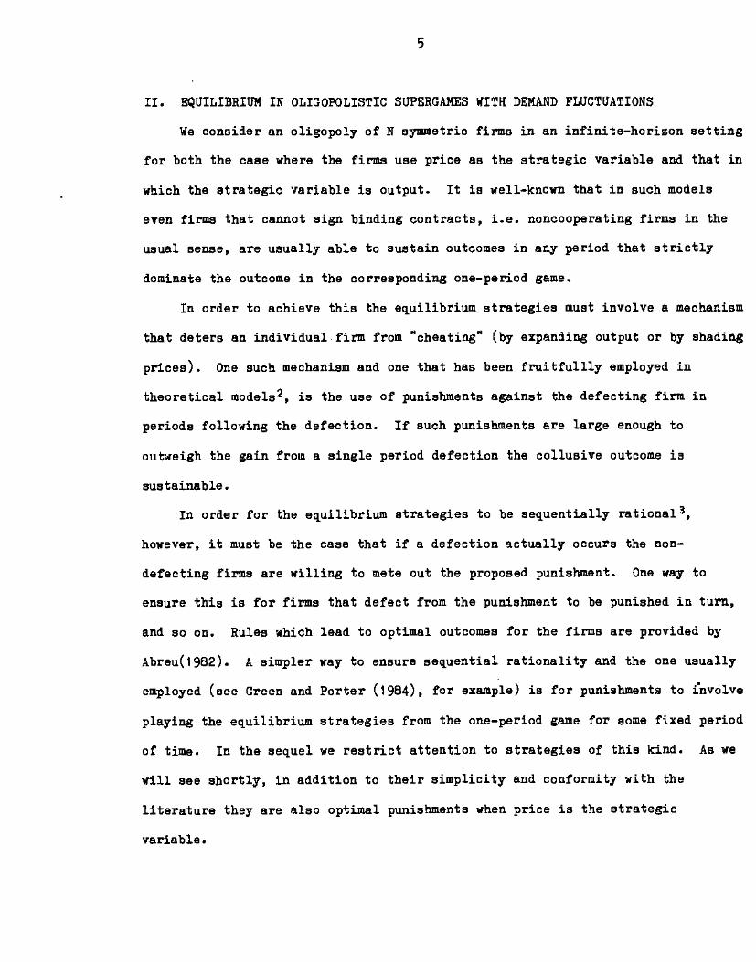
II. aQUILIBRIUM IN OLIGOPOLISTIC SUPERGAMES WITH DEMAND FLUCTUATIONS

We consider an oligopoly of N symmetric firms in en infinite—horizon setting

for both the case where the firms use price as the strategic variable and that in

which the strategic variable is output. It is well—known that in such models

even firws that cannot sign binding contracts, i.e. noncooperating firms in the

usual sense, are usually able to sustain outcomes in any period that strictly

dominate the outcorte in the corresponding one—period game.

In order to achieve this the equilibrium strategies must involve a mechanism

that deters an individual firm from "cheating" (by expanding output or by shading

prices). One such mechanism and one that has been fruitfuilly employed in

theoretical models2, is the use of punishments against the defecting firm in

periods following the defection. If such punishments are large enough to

outweigh the gain from a single period defection the collusive outcome is

sustainable.

In order for the equilibrium strategies to be sequentially rational3,

however, it must be the case that if a defection actually occurs the non—

defecting firms are willing to mete out the proposed punishment. One way to

ensure this is for firms that defect from the punishment to be punished in turn,

and so on. Rules which lead to optimal outcomes for the firms are provided by

Abreu(1982). A simpler way to ensure sequential rationality and the one usually

employed (see Green and Porter (1984), for example) is for punishments to Cnvolve

playing the equilibrium strategies from the one—period game for some fixed period

of time. In the sequel we restrict attention to strategies of this kind. As ye

will see shortly, in addition to their simplicity and conformity with the

literature they are also optimal punishments when price is the strategic

variable.

6

The major departure of our model from those that have previously been

studied is that we allow for observable shifts in industry demand, We denote the

inverse demand function by where is the industry output in period t

and c is the random variable denoting the observable demand shock (with

realization in period t). Ye assume that increases in St result in higher

prices for any t' that £ has domain [, ] and a distribution function F( c) and

that these are the same across periods (i.e. shocks are i.i.d.). Ye denote firm

i's output in period t by so that

— ii 1'The timing of events is as follows: At the beginning of the period all

firms lean the realization of (more precisely s becomes common knowledge).

Firms then simultaneously choose the level of their choice variable (price or

uantity). These choices then determine the outcome for that period in a way

that depends on the choice variable: in the case of quantities the price clears

the market given in the case of prices the firm with the lowest price sells

as much as it wants at its quoted price, the firm with the second lowest price

then supplies as much of the remaining demand at its quoted price as it wants,

and so on. The strategic choices of all the firms then become common knowledge

and this one—period game is repeated.

The force of the obsenability of St and the key to the difference between

the model and its predecessors is the following: The punishments that firms face

depend on the future realizations of c. The expected value of such punishments

therefore depends on the expected value of c. However the reward for cheating in

any period depends on the observable s. We show that for a wide variety of

interesting cases the reward for cheating from the joint profit—maximizing level

7

is nonotonically increasing in If is large enough, the temptation to

cheat outweighs the punisbaent." Being cognizant of this fact, an

implicitly colluding oligopoly settles on a profit below the fully collusive

level in periods of high demand so as to adequately reduce the temptation to

cheat. Such moderation of its behavior tends to lower prices below what they

would otherwise be, and may indeed cause them to be lower than for states with

lower demand. Ye illustrate this phenomenon for both prices as well as for

quantities as strategic variables.

(a) Price as the strategic variable

We begin with an analysis of the case in which marginal costs are equal to a

constant c. We demonstrate that the baste characteristics of our analysis are

not dependent on this assumption by means of an example below.

Let us point out at the outset that there always exists an equilibrium in

which all the firms set P=c in all periods. In this competitive case firma

expect future profits to be zero whether they cooperate at time t or not.

Accordingly the game at time t is essentially a one—shot game in which the unique

equilibrium has all firms setting Pc. In what follows we concentrate instead on

the equilibria that are optimal for the firms in the industry.

We begin by examining joint profit—maximization and the benefits to

unilateral defections from it. Define rf(Q(e),e) to be the profit of an

individual firm in state if the firms each produce qa which equals 1/N of the

joint profit—maximizing output, qm If a firm deviates from this proposed

outcome it can earn approximately NI? by cutting price by an arbitrarily small

amount and supplying the entire market demand. Firm i would therefore deviate

from joint profit—maximizing output if

NrIm(Qt(et),ct) — > i.e. if d(Q(e),e) >K(ct)/(N_1)

8

where K1(t) is the punishment inflicted on firm i in the future if it deviates

at time t.

The value of K±(s) depends on both the expected level of future profits if

there is no deflation at time t and on the nature of the punishment. Since we

want to concern ourselves with equilibrium strategies that are optimal for the

oligopoly and hence are interested in maintaining profits that are as large as

possible, we concentrate on punishments that are as large as possible; namely

those that have Pc for all t following a defection. While infinite punishment

periods are extreme they are subgaxne perfect and need not actually be implemented

in equilibrium. If the industry members change over time, however, infinite

length punishments are not compelling. To moderate the effect of this assumption

in the calculation of specific examples, we use reduced levels of the discount

rate, 8.

Suppose that the level of firm profits that can be sustained in a period

with state is K(ct)) when the punishment is K(e). Then using infinite

length punishments, the discounted future value of profits, and hence the

punishment, is

f flS(S K(c'fldF(&). (I)

Since the right hand side of (i) is independent of Ct. the punishment is

independent of the state and can be written merely as K.

Since 4) > 4) for all 4 >4, TI(Q, 4)

= 4)_c)Q >

4)_c)Q — c). Therefore, for given K, there is some highest level

of demand shock, c(K), which (N_1)?(Q(et),c). K.

This means that for ! Ct, the monopoly outcome is sustainable so that

K) — flm(Q(), By contrast, for e .?. an individual

9

firm has an incentive to cheat unless

K) — — t(Q(e), e). (2)

Of course IC in turn depends on from Euatton (1). In particular we have

•-g [f &Qt(ct). s)dF(t) + (i+r("Dif(q"(€'), t)I.s (3)

Thus we have a mapping from the space of possible punishments into itself: agiven punisbment impliei a cutoff e which in turn implies a new punishment from

(2). An equilibrium is a tired point of this mapping.

It remains to provide sufficient conditions for the existence of such a

fixed point i.e., to show there exists an c E (c, ) for whicht

Um(Qm(;), e) — K(s)/(N—1) — us (e, ICce:)). Let

g(4) a(N_1)r?(Qt(4), 4)

— Ic(4) (4)

where a is o/(i—o).

We need to show there exists an 4 (e, D such that g(4) — 0.

Equations (2) and (3) imply that

a(1—F(c'flK(c')— ft ?4). 4)dF(et) + (N—I)

C,

a ft ?(Q(e), e)dF(e)or, K(4) =

(1 a/(N—i) — aF(e')/(N—I)) (5)

rP(Q(e), e)Therefore, using (4) and (5) liii e(4) (n—i) ?(Q(). ) — ___________

C t.!which is negative if N < (i÷o)/((i—o) (Condition (i)).

At the other extreme,

g(t) — (N—1)tf'(Q(t), ) — a f:!r1(Q(C),C)dF(C) >0

10

if nm(Q(), -/f: I? (Q, £t)dP(tt) > WO'—i) (condition Cii)).

If Conditions ft) and (ii) hold, we have:

(a) g(4) is continuous, (b) g() > 0, and Cc) urn g(e') C 0, which imply the

existence of an 4€ Ce, ) such that g(4) 0 as required.

Conditions Ci) and (ii) have intuitively appealing interpretations.

Condition Ci) ensures that the firms are not tempted to "cheat" from the joint

profit—maximizing output in all states. This requires that N not be "too" large

relative to the discount rate. the larger is the discount rate (so that the

future is more important and hence the effect of the punishment is greater) the

larger the nwnber of firma the industry is able to support without a complete

breakdown in discipline.

Condition (ii) ensures that the monopoly outcome is not the only solution in

every state. This follows when there is sufficient dispersion in the

distribution or profit maximizing outputs. Clearly if there is no dispersion,

then for large enough punishments there is never any incentive to cheat. The LHS

of condition (ii) is a measure of the dispersion of profits.

Although g(c') is continuous it is not necessarily monotone. As a result

there may be multiple values of e' for which g(e') 0. Since we are concerned

with optimal schemes from the point of view of the firms in the industry, we

concentrate on the greatest such value.

There are several interesting features of this equilibrium. First note that* 5 El Ut * •

fore ) c we have liCe, Ic) il((Q Ce), c ). Yhen r?(e, K) is sot t t tt t

con8trained, must be as high as possible without reducing firmprofits below

the sustainable level. By the definition of the lf( .), if is lower

Ii

and P is higher an individual firm has an incentive to shade price slightly and

supply the industry demand. When Ct goes up, Q must go up ifCt)

is toremain constant since P is increasing in Ct and decreasing in Q. Moreover, if

is held constant at a level above a, the profits from deviating increase.

Therefore P must fall. Beyond c, prices fall monotonical].y as increases.

Below the oligopoly charges the monopoly price thus P tends to increase with

The model behaves as intuition would suggest with respect to changes in the

relevant parameters. Note firstly that the equilibrium value of IC is decreasing

in N. Therefore, given (2) ?(Q(e), is also decreasing in N. Thus the set

of states in which the monopoly outcome is sustainable is strictly decreasing in

N. In contrast to traditional models of oligopolistic interaction in which

oligopolies of all sires are always unable to achieve perfect collusion, the

firma in this model are usually able to do so for a range of states of demand.

However, as in Stigler's model (1964) the degree of implicit collusion varies

inversely with N.

As & decreases so that the future becomes less important, the equilibrium

value of K decreases and hence the sustainable level of profits and the set of

states in which monopoly profits are sustainable also shrinks.

As was mentioned above, punishments are never observed in eauilibrium. Thus

the oligopoly doesn't fluctuate between periods of cooperation and noncooperation

as in the models of Green and Porter (1984) and Porter (1983b). This arises

because of the complete observability of Ct. To provide an analagous model to

those just mentioned, we would have to further restrict the strategy space so

that the oligopoly can choose only between the joint monopoly price and the

12

competitive price. Such a restriction is intuitively appealing since the

resulting strategies are much simpler and less delicate. With this restriction

on strategies the firras know that when demand is high the monopoly outcome cannot

be maintained. They therefore assume that the competitive outcome will emerge,

which is sufficient to fulfill their prophecy. In many states of the world theoligopoly will earn lower profits than under the optimal scheme we have analyzed.

As a result, since punishments are lower, there will be fewer collusive states*

than before. There will still be some cutoff, e, that delineates the

cooperative and noncooperative regions. In contrast to the optimal model,

however, the graph of price as a function of state will exhibit a sharp decline

after with P c thereafter.

The above models impose no restrictions on the demand function except that

it be downward sloping and that demand shocks move it outwards. However the

model does assume constant marginal costs. The case of increasing marginal cost

is more complex than that of constant marginal costs for three reasons: (i) A

firm that cheats by price—cutting does not always want to supply the industry

demand at the price it is charging. Specifically, it would never supply an

output at which its marginal cost exceeded the price. So whereas before cheating

paid off when (N_1)1f'(s, K) > K now it pays off when if(c, K) > ri'(s, KP) — IC

where It"(et, IC, ) is the profit to the firm that defects when its opponents

charge P; (2) If a firm is to be deterred from cheating it must be the case that

ri5(e, K, I') — &'(c,, IC, P) — K i.e., the sustainable profit varies by state (incontrast to the marginal cost case). (3) With increasing marginal cost cheating

can occur by raising as well as by lowering prices. If its opponents are

unwilling to supply all of demand at their quoted price a defecting firm is able

to sell some output at higher prices.

17

A few results can nonetheless be demonstrated. First suppose that deviating

firms do not meet all of demand. Instead the output which equates the monopoly

price to their marginal cost is less than demand. this occurs when N is large

and when marginal costs rise steeply. Then the deviating firms equate P(Q,and o(q) where c' is the derivative of total costs with respect to output By

the envelope theorem the change in the deviants profit from an increase in isd in in It

_____________ ctet.d

. The change in profits from going along ii d ItCt ct

is thus smaller, ensuring that deviations become more tempting as Ct rises.

However, in this case, if the oligopoly keeps its price constant in response to

the increase in the desire to deviate actually falls. This occurs because

when the price is constant the profits from deviating are constant. Instead,

since the oligopoly price exceeds marginal cost, an increase in s accompanied by

a constant price raises the profits from going along.

When deviating firma meet all of demand the analysis is zore difficult. For

this case we consider an example in which demand and marginal costs ate linear:

Pa+ et_bct (6)— + dq/2 (7)

Then monopoly output and price are: 6

Qat(a+c_c)/(2b+d/N) (a)

= E(a + c)(bN + d) + bNc]/(2bN • d) (9)

If deviating firms could sell all they wanted at a price a shade below

they would equate (c+dq) to P. This would lead to output equal to

it - [(a + - c)(b + d/N)]/[d(2b + a/N)] (10)

¶4

The actual output of the deviating firm, is the minimum of q and qm• So the

deviating firm meets demand as long as b is bigger than or equal to (N—OdIN.

Marginal coat must not rise too rapidly and N must not be too big.

When the deviating fin meets demand its profits are:

rn + Nd(1—N)(q"52/2 (ii)

The change in I?' from a change in is simply qm• Therefore using (a) the

change in the benefits from deviating is:

d([Id_[ld) — (N-i )q(2bN — d(N—1)(12)

act (2bNtd)

which is positive when demand is met, Cheating becomes more desirable as

rises. If the oligopoly is restricted to either collude or compete, high

will generate price wars. Alternatively the oligopoly can pick prices p5 which

just deter potentially deviating firms. These prices equate U5, the profits from

going along, with — K where K is the expected present value of minus the

profits obtained when all firms set price equal to marginal cost.

Since q'1 is linear in p8 whether deflating firms meet demand or marginal

d a. ii. Scost, 11 is quadratic in P in both cases. U is also quadratic in P . For a

given IC one can then find in the states that do not support monopoly by

solving two quadratic equations. The relevant root is the one with the highest

value of [j8 which is consistent with the deviating firms planning to meet demand

or marginal cost. The resulting P5'a then allow one to find a new value for K.

One can thus iterate numerically on K starting with a large number. Since larger

values of K induce more cooperation the first K which is a solution to the

iterative procedure is the best equilibrium the oligopoly can enforce with

competitive punishments. Figure 1 graphs these equilibrium prices and compares

PR

ICE

A

S

A

ST

RA

TE

GIC

VA

RIA

BLE

P

arameters; a=

60,b=1,c=

O,d=

1/3.&.7,N

5

4) U

L 0

75

70

65

60

55

50

45

40

35

30

25 0 10

20 30

40 50

60 70

State

80

15

theTA to the monopoly prices as a function of states for a specific configuration

of parameters. In particular c is uniforlrLly destributed over (o,i,... ,ao}.

As before the price rises monotoni.oally to St and then falls. The majOr

difference here is that eventually the price begins to rise again. The

explanation for this is straightforward. For high values of the equilibrium

value of P is such that a deviating firm would increase its output only until P

equals its marginal cost; it is not willing to supply all that is demanded at its

lower price. An improvement in demand from this level accompanied by a constant

price actually reduces the incentive to cheat. Thus the oligopoly can afford to

increase its prices somewhat.

b) Quantities as strategic variables.

There are two differences between the case in which quantities are used as

strategic variables and the case in which prices are. First, when an individual

firm considers deviations from the behavior favored by the oligopoly, it assumes

that the other firms will keep their quantities constant. The residual demand

curve is therefore obtained by shifting the original demand curve to the left by

the amount of their combined output. Second, when firms are punishing each other

the outcome in punishment periods is the Cournot equilibrium.

The results we obtain with quantities as strategic variables are somewhat

weaker than those we obtained with prices. In particular it is now not true that

any increase in demand even with constant marginal costs leads to a bigger

incentive to deflate from the collusive level of output. However, we present

robust examples in which this is the case. We also show with an example that

increases in demand can, as before, lead monotonically to "more competitive"

behavior. -

16

We show that increases in demand do not- necessarily increase the incentive

to deviate by means of a counterexample. Suppose that deaand is characterized by

constant elasticity and that a demand shock moves it horizontally from state 4

to state 4. In this setup the collusive price is the same in both states.

Therefore any firm that produces the collusive output sells more in state than

in state 4. The residual demand curves the firm faces are therefore as

represented in Figure 2. A deviating firm chooses output to maximize profits

given these residual demand curves. Suppose that this maximum is achieved at

output D and price d for state c. For this to be a worthwhile deviation it

must be the case that the revenues from the extra sales due to cheating (CD) are

greater than the loss in revenues on the old sales from the decrease in pricea dfrom P(Q ,.) to P • But (except for a horizontal translation) the firm faces the

same residual demand curve in both states. Thus by selling at d, the extrasales due to cheating are the same at 4 (As) than at s (CD). Moreover the loss

in revenue on old sales is strictly smaller at 4. Therefore the firm has a

strictly greater incentive to deviate in state 4 than in state 4.

The above counterexanple exploits the assumption of the constant elasticity

of demand only to establish that the collusive price is the same in both states.

We have therefore also proved a related proposition: if the oligopoly keeps its

price constant when increases (thus supplying all the increased demand), the

incentive to cheat is reduced when demand shifts horizontally. Thus in the

examples we provide below, the oligopoly is able to increase the price as the

state improves.

Suppose that, instead, demand and costs are linear as in (6) and (7). Then

an increase in c always leads to a bigger incentive to deviate from the

collusive output. This can be seen as follows. Suppoee that in this case the

P(Qm..)

FIGURE 2

The Incentive to Deviate withQuantities as the Strategic Variable

0 A B C D Q

P

(Qm,s)

17

oligopoly agrees that each firm should produce q. The deviating firm therefore

maximizes:

rid — q [a + — c —b((N—1)q + q)J — dq/2 (t)

with respect to So its output is:

— [a +Ct

— c — b(N—1)q]/(2b + d) (14)

The derivative of at the optimum with respect to is

Therefore, using (a), the derivative of the benefit from deviating from the

collusive output in any one period is:

d(t1" — If') —[b(N_l)]2(a+c_c)

det (d+2bu)2(2b+ d)

which is always poBitive. Deviating becomes more tempting as increases,

independently of b and d, as tong as both are finite. Therefore in the repeated

setting as long as the discount rate is not too large or N too small, individual

firms will deviate from the collusive outcome when demand is high. This leads to

price wars when the only options for the oligopoly are to either compete or

collude.

Alternatively the oligopoly can choose a level of output q5 that will just

deter fins from deviating when demand is high. These levels of output can be

obtained numerically in a manner analogous to the one used to obtain the in

the previous subsection. These outputs equate fl0, the profits from going along,

to crid — K) where K is the expected discounted difference between us and the

profits from the Cournot equilibrium. By substituting (16) in (13) 11d becomes

quadratic in q5. Since is also quadratic in q8 the q°'s are obtained as

solutions to quadratic equations for given IC.7 The resulting q8's allow us to

compute a new value of K. By iterating in a manner analagous to the one used to

Ia

derive Figure 1 we obtain the best equilibrium for the oligopoly. Figure 3 plots

the ratio of this ui1ibrium price to the monopoly price as a function of

While a variant of the argument made earlier guarantees that equilibrium price

rises as c rises, it can be seen that beyond a certain Ct the ratio of

equilibrium price to monopoly price falls monotonically.

Monopoly Price/Oligopoly Price

0CH

vrII

I!'2J

oJErn

0

000000000PooD(Dco (0 bO(0 fJ (, 4 0' 0' '4 (0 ..a —

-a0

0

cJJ0

C')

CD

(1'0

0

—I0

a

19

III. BUSINESS CYCLES

So far we have considered only the behavior of an oligopoly in

isolation. For this behavior to form the foundation of business cycles

we need to model the rest of the economy, While the principle which

underlies these business cycles is probably quite general we illustrate

it with a simple example. Ye consider a "real" two sector general

equilibrium model in which the first sector is competitive while the

other is oligopolistic. There is also a competitive labor market. To

keep the model simple it is assused that workers have a horizontal supply

of labor at a wage equal to the price of the competitive good. Since

the model is homogeneous of degree zero in prices, the wage itself can be

normalized to equal one. So the price of the good produced competitively

must also equal one. This good can be produced with various combinations

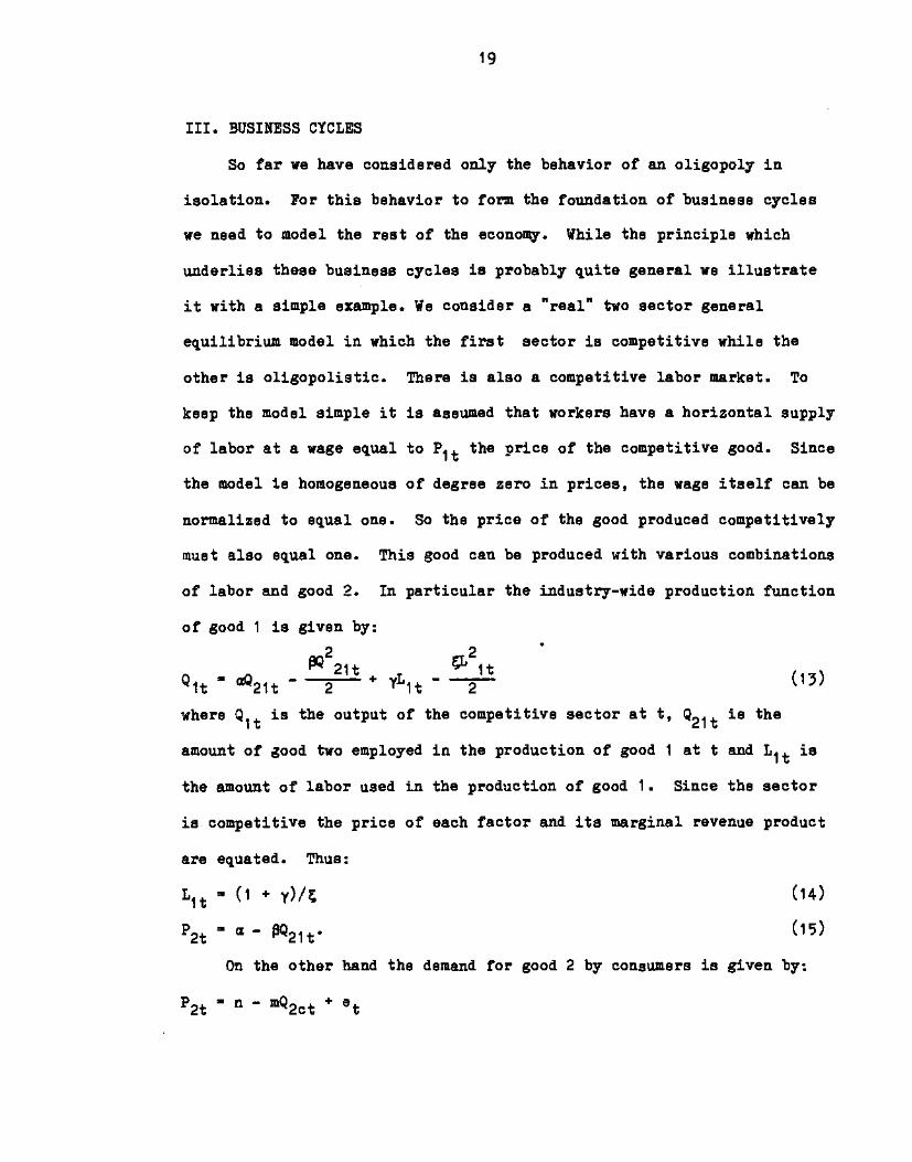
of labor and good 2. In particular the industry—wide production function

of good 1 is given by:

lt — 21t —2

+ yLit —2 (13)

where is the output of the competitive sector at t, is the

amount of good two employed in the production of good 1 at t and Lit is

the amount of labor used in the production of good 1. Since the sector

is competitive the price of each factor and its marginal revenue product

are equated. Thus:

Lit— (1 + y)/ (14)

— 2lt' (15)

On the other hand the demand for good 2 by consumers is given by:

2t — n — 2ct +

20

where 20t is the quantity of good 2 purchased by consumers, n and in are

parameters and e is an i.i.d. random variable. Therefore total demand

for good 2 is given by:

2t — a + — bQ2t

a — (lip + my)/(m • p) a +p) (6)

b - mp/(m + p)

Note that equation (16) is identical to equation (6). To continue

the parallel with our sections on partial equilibrium we assume that the

labor requirement to produce 2t is:

L — cQ +2t 2t ' / 2t

which implies that, as before, marginal cost is c +dQ2t.

The model

would be unaffected if good 1 were also an input into good 2 since is

always equal to the wage. If sector 2 behaved competitively marginal

cost would equal Then output of good 2 would be while price

would be

— (a + — c)/(b/2 + d)

— ((a +c)d

+ bc/2)/(b/2 + d)

An increase in raises both the competitive price and the

competitive quantity of good 2. By (15) less of good 2 will be used in

the production of good I thus leading to a fall in the output of good 1.

a shift in tastes raises the output of one good and lowers that of

the other. The economy implicitly has, given people's desire for

leisure, a production possibility frontier.

Similarly, if sector 2 always behaves like a monopolist, output and

price are given equations (s) and (9) respectively. Therefore increases

in raise both 2t and 2t thus lowering Q• Once again shifts in

21

demand are unable to change the levels of both outputs in the same

direction. On the other hand if the industry behaves like the oligopoly

considered in the previous sections, an increase in etoan easily lead to

a fall in the relative price of good 2. This occurs in three out of the

four scenarios considered in previous sections. It occurs when the

unsustainability of monopoly leads to competitive outcomes whether the

strategic variable is price or output as long as increases in make

monopoly harder to sustain. It also always occurs when the strategic

variable is prices and the oligopoly plays an optimal supergame. The

decrease in in turn leads firms in the first sector to demand wore of

good 2 as an input and to increase their output. So, a shift in demand

towards the oligopolistic goods raises all outputs much as all outputs

move together during business cycles.

A number of comments deserve to be made about this model of business

cycles. First our assumption that the real wage in terms of good I is

constant does not play an important role. In equilibrium the reduction

in raises real wages thus inducing workers to work more even if they

have an upwardly sloping supply schedule for labor. Thether this

increased supply of labor would be sufficient to meet the increased

demand for employees by sector 2 is unclear. If it wasn't the wage would

have to rise in terms of good 1. Nore interestingly if the increased

supply of labor was large, would have to rise thus increasing

employment also in sector I • This would lead to an expansion even if

good 2 was not an input into good 1. This pattern of price movements is

consistent with the evidence on the correlation between product wages and

employment presented below.

22

Second, the model can easily be made consistent with the procyclica].

variation of profits. Even though sector 2 reduces the margin between

price and marginal cost as output expands, the difference between

ravennes and total costs can increase as long as there are fixed coats.

Third, it is luite plausible that changes in financial variables

like the money stock and interest rates lead shifts in the composition of

demand. For instance increases in the money stock might be associated

with lower interest rates and a higher demand for durable goods. As

shown below, durable good industries appear to be more oligopolistic than

other industries. These shifts in demand form a large part of the

informal discussion surrounding the ¶983 recovery in the US , for

example.

Random shifts in demand have already been showed to cause movements

in employment in the asymetric information model of Grossman, Hart and

Maskin (ige3). However, contrary to the claims of Lilien (1982) such

random sectoral shifts do not appear to be correlated with agregate

fluctuations. Instead Abraham and Katz (1984) show that different

sectors only have distinct correlations with agregate output. Moreover

the sectors whose output is more correlated with agregate output appear

to have a higher rate of growth on average. This leads to the

statistical illusion that when output grows faster, as in a recovery,

there is more intersectoral variance in output growth then when output

growth is small, as in a recession. Note that Abraham and Katz's finding

that some sectors are more "cyclic" than others accords well with our

theory that shifts towards oligopolistic sectors are necessary to expand

aggregate output. This finding also appears to be somewhat at odds with

the literature on real business cycles (Long and Plosser (1983) and King

23

and Plosser (1984)). In this literature expansions are caused by

favorable unobservable technological shocks. Aside from the fact that

there is no independent evidence for the importance of these shocks and

that they do not appear in the casual discussions of the poop1. who are

directly affected by business cycles it is somewhat peculiar that these

favorable shocks always recur in the same "cyclic" industries.8

Our model also sheds light on some slightly unfashionable concepts

of Keynesian economics. One of the most pervasive facts about increases

in the money supply is that they are not accompanied by equiproportional

increases in prices. Prices appear to be sticky (of Rotemberg (1982)).

Suppose that, increases in St are correlated with increases in the money

supply. Then increases in output are correlated with increases in the

money supply. As long as increases in output raise the demand far real

money balances, increases in the money supply will be correlated with

increases in real money balances. Prices do not rise equipropor—

tionately. A second concept we can usefully discuss in the context of

our model is that of a multiplier. This concept reflects the idea that

increases in demand lead output to rise which then leads to further

increases in demand. Here a shift in demand towards an oligopolistic

sector can raise that sector's output, lower its prices and thus raise

national income. In turn this increased national income can lead tqincreases in the demand for other goods produced in oligopolistic markets

thus lowering their prices and raising their output as well. This

process can continue until almost all oligopolistic markets have lower

prices.

24

IV. SOME RELEVMJT FACTS

a) The folklore

The theory presented in section II runs counter to the industrial

organization folklore. This folklore is best articulated in Scherer

(1980 p.208) who says: "Yet it is precisely when business conditions

really turn sour that price cutting runs most rampant among oligopolists

with high fixed costs". Our attempt at finding the facts that support

this folklore has, however, been unsuccessful. Scherer cites three

industries whose experience is presented as supporting the folklore.

These are rayon, cement and steel. For rayon he cites a study by Narkha

(1952) which shows mainly that the nominal price of rayon fell during the

Great Depression. Since broad price indices fell during this period this

is hardly proof of a price war. Rayon has since been replaced by other

plastics making it difficult to use postwar data to check whether any

real price cutting took place during postwar recessions. For steel

Scherer in fact admits the following: "... up to 1968 and except for some

episodes during the 1929—38 depression, it was 'sore successful than

either cement or rayon in avoiding widespread price deterioration, even

when operating at less than 65% capacity between 1958 and 1962 (p. 210).

This leaves cement. Ye study the cyclical properties of real ceient

prices below. To do this we collected data on the average price of

portland cement from the Minerals Yearbook published by the Bureau of

Mines. We then compare this price with the Producer Price Index and the

price index of construction materials published by the Bureau of Labor

statistics. Regressions of the yearly rate of growth of real cement

prices on the contemporaneous rate of growth of OTU' are reported in Table

25

1. The coefficient of the rate of growth of GUI is always meaningfully

negative. A 1% increase in the rate of growth of ON? leads to a 0.5—1.0%

fall in the price of cement. To test whether the coefficients are

significant the regression equations must be quasi—differenced since

their Durbin—Yatson statistics are small. Indeed the coefficients are

all significantly different from zero at the five percent level. More

casually, the real price of cement rose in the recession year 1954 while

it fell in the boom year 1955. similarly, it rose during the recession

year 1958 and fell in 1959.

These results show uniformly that the price of cement has a tendency

to move countercyclically as our theory predicts for an oligopoly. These

results are of course not conclusive. First, it might be argued that the

demand for cement might be only weakly related to ON?. Without a

structural model, which is well beyond the scope of this paper, this

auestion cannot be completely settled. The rate of growth of the output

of the cement industry has a correlation of .69 with the rate of growth

of ON? and of .77 with the rate of growth of construction activity

which is well known to be procyclical. However, these correlations are

not sufficient to prove that cement is "more procyclical" than the

tical sector included in GNP. Second our regressions do not include

all the variables one would expect to see in a reduced form. Thus the

effect of GNP might be proxying for an excluded variable like the

capacity of cement mines which Scherer would probably expect to exercise

a negative effect on the real price of cement. While this is indeed a

possibility it must be pointed out that capacity itself is an endogenous

variable which also responds to demand. It would thus be surprising if

enough capacity were built in a boom to more than offset the increase in

Table I

THE CYCLICAL PROPERTIES OF CEMENT PRICES

Yearly Data from 1947 to 1981

DependentVariable

Coefficient

pC/pp PC/PPI pC/pCOE pC/pOOfl

Constant

GNP

p

1t2

D.W

.025(.010)

—.438(.236)

.10

1.07

.025(.012)

—.456(.197)

.464(.173)

.15

1.73

.038(.007)

—.875(.161)

.48

1.28

.037(.008)

—.816(.149)

.315(.ia)

.52

1.92

C conP is the price of cement, PH is the producer price index and P isthe price index of construction materials. Standard errors are inparenthesis.

26

demand. If anything, the presence of costs of adjusting capacity would

make capacity relatively unresponsive to increases in GNP.

b) Actual price wars

There have been two recent studies showing that some industries

alternate beetween cooperative and noncooperative behavior. The first is

due to Bresnahan (1981). Ne studies the automobile industry in 1954,

1955 and 1956. He tries to evaluate the different interpretations of the

events of 1955. That year production of automobiles climbed by 45% only

to fall 44% the following year. Bresuahan formally models the automobile

industry as carrying out two sequential games each year. The first

involves the choice of models and the second the choice of prices. He

concludes that the competitive model of pricing fits the 1955 data taken

by themselves while the collusive model fits the 1954 and 1956 data.

Those two years exhibited at be8t sluggish GNP growth. GNP fell. 1% in

1954 while it rose 2% in 1956. Instead 1955 was a genuine boom with GNP

growing 7%. Insofar as cartels can only sustain either competitive or

collusive outcomes, this is what our theory predicts. Indeed, in our

model, the competitive outcomes will be observed only in booms.

Porter (1983b) studies the railroad cartel which operated in the

1880s on the Chicago—New York route. He uses time series evidence (as

opposed to the cross section evidence of Bresnahan) to show that some

months were collusive while others were not. His theory which is

developed in Green and Porter (1984) is that the breakdowns from the

collusive output ought to occur in periods of unexpectedly low demand.

He finds no support for this theory from the residuals of his estimated

equations. Instead, we will argue his results support out theory. Table

2 presents the relevant facts. The first three columns are taken from

Porter's paper. The first

Table 2

RAILROADS IN THE 1680's

EstimatedNonadherence

RailShipaents

(MillionBushels)

FractionShipped

by Rail

Total GrainProduction(Billion

Tons)

Days LakesClosed from4/I — 12/3t

1880

1881

1882

1883

1884

1885

1886

0.00

0.44

0.21

0.00

0.40

0.67

0.06

4.13

7.68

2.39

2.59

5.90

5.12

2.21

22.1

50.0

13.8

26.8

34.0

48.5

17.4

2.70

2.05

2.69

2.62

2.98

3.00

2.83

35

69

35

58

58

61

50

27

column shows an index of cartel nonadherence estimated by Porter. He

shows this index paralells quite closely the discussions in the Railway

Review and in the Chicago Tribune which are reported by IJien (1978). The

second column reports rail shipments of wheat from Chicago to New

York. The third column shows the percentage of wheat shipped by rail

from Chicago relative to the wheat shipped by both lake and rail. The

last two columns are from the Chicago Board of Trade Annual Reports. The

fourth column presents the national production of grains estimated by the

Department of Agriculture. This total is constructed by adding the

productions ot' wheat, corn, rye, oats and barley in tons. This

aggregation is not too difficult to justify since the density of

different grains is fairly similar. Finally the last column represents

the number of days beetween April 1 and December 31 that the Straits of

Mackinac remained closed to navigation. (They were always closed

beetween January 1 and March 31.) Such closures prevented lake shipments

of grain.

As can readily be seen from the table the three years in which the

most severe price wars occurred were 1881, 1884 and 1885. Those are also

the years in which rail shipments are the largest both in absolute terms

and relative to lake shipments. This certainly does not suggest that

these wars occurred in periods of depressed demand. However, shipments

may have been high only because the railroads were competing even though

demand was low. To analyze this possibility we report the values of two

natural determinants of demand. The first is the length of time during

which the lakes were closed. The longer these lakes remained closed the

larger was the demand for rail transport. This is the only demand

variable included in Porter's study. The lakes were closed the longest

28

in 1881 and 1885. These are also the years in which the index of cartel

nonadnerence is highest. In 1883 and 1884 the lake, remained closed only

slight].y less time than in 1885 and yet there were price wars only in

1884. The second natural deterainant of demand, total grain production,

readily explains the anomalous behaviour of 1883. This was also the year

in which the total grain production was the second lowest in the entire

period and in particular, was 12% lower than in 1884. This must have

depressed demand so much that, in spite of the lake closings, total

demand for rail transport was low enough to warrant cooperation. A

number of objections can be raised against this interpretation of

Porter's facts. First, Porter used weekly data instead of our annual

aggregates and it might be thought that weekly data provide a stronger

basis for accepting or njeoting our theory. In fact, however, the price

wars followed a seasonal time pattern. The first price war started

around January 1881 and lasted for the whole year. The second price war

started around January 1884 and ended at the end of 1885. Ye suspect

that around midwinter agents could form a fairly accurate prediction of

the opening of the lakes by studying the thickness of the ice. If they

expected the lakes to be closed for a long period they naturally expected

a price war to develop. Once the individual railroads predicted a war

for the future they were tempted to cut their prices loediatly for two

reasons. First, the penalties for deviating wore reduced since in the

future the outcome will be competitive in any event. Second, individuals

who had the capacity to store grain would postpone shipments if they knew

a price war was imminent thus lowering even the monopoly price. The

presence of such storage facilities would also seem to make

identification of the weekly changes in demand difficult. On the other

29

hand years with high grain production or with a short lake shipping

season will nonetheless be years of high demand.

The second objection to our analysis is that we use aggregate

production in the entire United States as our proxy for grain production

in the Chicago region. The reason for this is that it is very difficult

to define the Chicago region. It clearly includes more than the state

of Illinois but less than our proxy. In any event the movements in total

production figures represent mostly movements in the production of the

grain belt which includes Illinois.

c) Price—cost margins

One natural test of our theory is whether there is substantial price

cutting by oligopolists when demand is high. What is difficult about

carrying out this test is that prices must be compared to marginal costs

and that data on marginal costs at the firm or even at the industry level

is notoriously scarce. Traditionally researchers in Industrial

Organization have focused on price—cost margins which are given by sales

minus payroll and material costs divided by sales. This is a crude

approrimation to the Lerner Index which has the advantage of being easy

to compute. Indeed Scherer cites a number of studies which analyzed the

cyclical variability of these margins in different industries. These

studies have led to somewhat mixed conclusions. However Scherer

concludes on p.35?: "The weight of the available statistical evidence

suggests that concentrated industries do exhibit somewhat different

pricing propensities over tine than their atomistic counterparts. They

reduce prices (and more importantly) price—cost margins by less in

response to a demand slump and increase them by less in the boom phase".

This does not fit well with the folklore which would predict that on

30

average prices would tend to fall more in recessions the more

concentrated is the industry. Our theory would explain these facts as

follows. It repiires that prices fall relative to marginal cost in

booms. This is consistent with rising price cost margins as long as some

of the expenditure on labor is in fact a fixed cost. this can be seen as

follows: Suppose that price and marginal cost are constant and that

there are some fired costs. Then if the labor costs include some fired

costs an increase in output will lower the importance of these fixed

costs thus raising price—cost margins. The key is that price—cost

margins rise by less in concentrated industries. So either the fixed

costs are less important in the concentrated industries, which seems a

priori unlikely, or the concentrated industries tend to reduce prices

relative to marginal cost.

We also study some independent evidence on margins. Thirds (1984)

reports correlations between employment and real product wages in various

two digit industries. These real product wages are given by the average

hourly wage paid by the industry divided by the value added deflator for

the industry. They can be interpreted as a different crude measure of

marginal cost over, prices. Their disadvantage over the traditional

price—cost margin is that, unlike the latter, they not only require that

materials be proportional to output but also that materials costs be

simply passed on as they would in a competitive industry with this cost

structure. On the other hand, their advantage over the traditional

measure is that they remain valid when some of the payroll expenditure is

a fixed cost as long as, at the margin, labor has a constant marginal

product. Moreover it turns out that if the marginal product of labor

31

actually falls as employment rises our evidence provides even stronger

support for our theory.

The correlations reported by Burda for the real product wage and

employment using detrended yearly data from 1947 to 1978 are reported in

Table 3 which also reports the average four firm concentration ratio for

each two digit industry. This average is obtained by weighting each four

digit SIC code industry within a particular 2 digit SIC code industry by

its sales in 1967. These weights were then applied to the 1967 four firia

concentration indices for each 4 digit SIC code industry obtained from

the Census.9

PASLE 3CONCEN'TRATION MTh THE CORRELATION BEETYEEN REAL

•.tAGES MID E)LOfXENT

SIC# INDUSTRY DESIGNATION CORREL. CONCEN.

DURABLES MANUFACTURING24 Lumber and wood products —.33 17.625 Furniture and fixtures —.18 21.632 Stone, clay and glass .39 37.433 Primary metals .32 42.934 Fabricated metal industries .23 29.1

35 Machinery except electrical .12 36.336 Electrical and electronic equipment .34 45.0371 Motor vehicles and equipment .19 80.5372—9 other transportation equipment .02 50.138 Instruments and related products —.36 47.8

NONDURABLE MMIUYACTURING20 Food and Kindred products —.30 34.521 Tobacco manufactures —.64 73.622 Textile mill products .04 34.123 Apparel and related products —.53 19.726 Paper and allied products —.42 71.227 Printing and publishing .40 18.928 Chemical and allied products —.03 49.929 Petroleum and coal products —.48 32.930 Rubber .16 69.131 Leather and leather products —.44 24.5

32

At first glance it is clear front the table that more concentrated

industries like motor vehicles and electrical machinery tend to have

positive correlations while lees concentrated industries like leather,

food and wood products tend to have negative correlations. Statistical

testing of this correlation with the concentration index is, however,

somewhat delicate. That is because our theory does not predict that an

industry which is 5% more concentrated than another will reduce prices

more severely in a boom. On the contrary a fully fledged monopoly will

always charge the monopoly price which usually increases when demand

increases, All our theory says is that as soon as an industry becomes an

oligopoly it becomes likely that it will cut prices in booms. Naturally

the concentration index is not a perfect measure of whether an industry

is an oligopoly. Indeed printing has a 1.0w concentration index even

though its large components are newspapers, books and magazines which are

in fact highly concentrated once location in space or type is taken into

account. Nonetheless higher concentration indices are at least

indicators of a sinner number of important sellers. Glass is undoubtely

a more oligopo]istic industry than shoes. So we decided to classify the

sample into relatively unconcentrated and relatively concentrated and

chose, somewhat arbitrarily, as the dividing line the median -

concentration of 35.4. This lies between food and nonelectrical

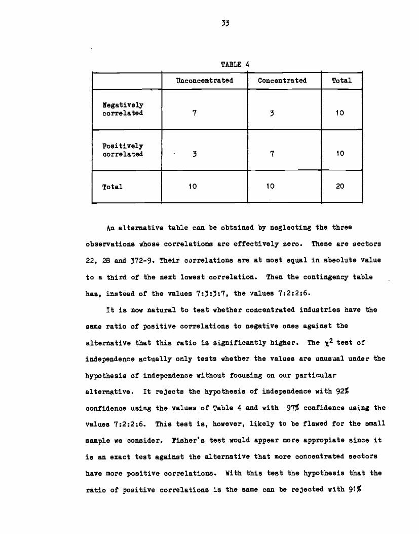
machinery. We can then construct the following 2X2 contingency table:

33

PABIiE 4

Unconcentrated Concentrated Total

Negativelycorrelated 7 3 10

Positivelycorrelated 3 7 10

Total 10 ¶0 20

An alternative table can be obtained by neglecting the three

observations whose correlations are effectively zero. These are sectors

22, 28 and 372—9. Their correlations are at most equal in abeolute value

to a third of the next lowest correlation. Then the contingency table

has, instead of the values 7:3:3:7, the values 7:2:2:6.

It is now natural to test whether concentrated industries have the

same ratio of positive correlations to negative ones against the

alternative that this ratio is significantly higher. The x2 test of

independence actually only tests whether the values are unusual under the

hypothesis of independence without focusing on our particular

alternative. It rejects the hypothesis of independence with 92%

confidence using the values of Table 4 and with 97% confidence using the

values 7:2:2:6. This test is, however, likely to be flawed for the small

sample we consider. Fisher's test would appear more appropiate since it

i8 an exact test against the alternative that more concentrated sectors

have more positive correlations. With this test the hypothesis that the

ratio of positive correlations is the sane can be rejected with 91%

34

confidence using the data of Table 4 and with 96% confidence using

7:2:2:6.

there is thus a fair amount of evidence for the hypothesis that more

concentrated sectors are more likely to have positive correlations. We

interpret this by imagining a world in which technology is subject to

technological progress at a constant rate and in which capital is

accumulated smoothly. The deviations of employment from its trend then

occur only in response to increased demand. Then if the firms behave

monopolistically the real product wage will tend to fall when demand

increases. The same will occur if the firms are competitive and the

marginal product of labor falls as employment rises. Particularly when

there are diminishing returns to labor the finding that the product wage

rises when employment rises suggests the widespread price cutting our

theory implies.

There are alternative explanations for our findings, however. The

first is that the positive correlations are due to monopolistic pricing

in the face of increasing returns to labor in the short run. The

existence of such increasing retuns strike us as unlikely. When

production is curtailed this is usually done by temporary closings of

plants or reductions of hours worked. These reductions would always

start with the most inefficient plants and workers thus suggesting at

most constant returns to labor in the short run. The second alternative

explanation relies on technological shocks. These shocks can, in

principle either increase or decrease the demand for labor by a

particular sector. If they increase the demand and the sector faces an

upwards sloping labor supply function, employment and real wages can both

increase. The difficulty with this alternative explanation is that the

35

sectors with positive correlations do not appear to be those which a

casual observer would characterize as having many technological shocks of

this type. In particular stone, clay and glass, printing and publishing

and rubber appear to be sectors with fair]j stagnant technologies. On the

other hand instruments and chemicals may well be among those whose

technolo- has been changing the fastest.

36

V. CONCLUSIONS

This paper basically consists of three parts. The first is a somewhat

novel theory of oligopolies in situations in which demand fluctuates.

The second is an analysis of the business cycles that such oligopolies

can induce, while the third is a study of the plausibility of the idea

that oligopolistic industries tend to behave more competitively in booms.

Since the data appear consistent With this idea they conaitute fairlydirect evidence in favor of both our theory of oligopoly and that of

business cycles. This suggests that both theories and their empirical

validation deserve to be extended.

The theory of oligopoly might be extended to include also

imperfectly observable demand shifts, prices and outputs. This type of

imperfect observability is the main concern of Green and Porter (1984)

who study markets with no observable shifts in demand. The advantage of

introducing unobservable shifts in demand is that these can induce

reversions to punishing behavior even when all firms are acting

collusively. A natural question to ask is whether reversions to

punishing behavior that result from unobservable shocks are more likely

when everybody expects the demand curve to have shifted out.

Unfortunately this appears to be a very difficult question to answer.

Even the features of the optimal supergame without observable shocks

discussed in Porter (1983a) are hard to characterize. Adding the

complication that both the length of the punishment period as well as the

price that triggers a reversion depend on observable demand is a

37

formidable task.

In this paper we considered only business cycles which are due

to the tendency of oligopolists to act more competitively when

demand shifts towards their products. An alternative and commonly held

view is that business cycles are due to changes in aggregate demand which

do not get reflected in nominal wages. In that case a decrease in

aggregate demand raises real wages thereby reducing all outputs. In our

theory of oligopoly, firms tend to collude more in these periods. Hence

recessions are not only bad because output is low but also because

mioroeconomic distortions are greater. This suggests that stabilization

of output at a high level is desirable because it reduces these

distortions.

On the other hand, the busine8s cycles discussed here do not

necessarily warrant stabilization policy. While models of real

business cycles merely feature ineffective stabilization policies

hers such policies might actually be harmfull. Booms occur because,

occasionally, demand shifts towards oligopolistic products. In these

periods the incentive to deviate from the collusive outcome is greatest

because the punishment will be felt in periods which, on average have

lower demand and hence lower profits. If instead future demand were also

known to be high, the threat of losing the monopoly profits in those good

periods might well be enough to induce the members of the oligopoly to

collude now. So, if demand for the goods produced by oligopolies were

stable they might collude always, leaving the economy in a permanent

recession. 10 Therefore the merits of stabilization policy hinge

crucially on whether business cycles are due to shifts in demand

38

unaccompanied by nominal rigidities or whether they are due to changeB in

aggregate demand accompanied by such rigidities. Disentangling the

nature of the shifts in the demand faced by oligolopies therefore seellia

tQ be a promising line of research.

Much work also remains to be done empirically validating our

model itself. In section iv we presented a variety of simple tests

capable of discriminating between the Industrial Organization folklore

and our theory. Since none of them favored the folklore it may well be

without empirical content. On the other hand, our theory desenee to be

tested more severely. First a more disagregated study of the cyclical

properties of price—cost margins seems warranted. Unfortunately, data on

valued added deflators does not appear to exist at a more disagregated

level so a different methodology will have to be employed. Second our

theory has strong implications for the behaviour of structural models of

specific industries. Th. study of such models ought to shed light on the

extent to which observable shifts in demand affect the degree of

collusion.

39

FOOTNOTES

11f firms find borrowing difficult, recessions might be the idealoccasions for large established firms to elbow out their smaller

competitors.

2See, for example, Friedman (1971), Green and Porter (1984) and Radner(1980).

3sequentially rational strategies are analysed in gaines of incompleteinformation by Kreps and Wilson (1952). For the game of completeinformation that we analyse we use Selten's concept of subgame perfection

(1965).

kIn an informal discussion, Kurz (1979) recognizes the link betweenshort—run profitability and the sustainability of collusive outcomes.However, the relationship between profits, demand, and costs is not make

explicit.5The argument of K, 4, in (3) should not be confused with that in (I).The latter represents the realization of the shock at t whereas theformer is the state beyond which monopoly becomes unsustainable.

61n this case an increase in can directly be interpreted as either ashift outwards in demand or a reduction in c, that part of marginal costwhich is independent of q. This results from the fact that the profit

functions depend on s only through (a+ st—c).

7The relevant root is the one with the highest profits for theoligopoly;

8The interoectoral pattern of output movements can be independent of thesector which has a technological shock if (as seems unlikely) goods areconsumed in fixed proportions which depend on the level of utility only.Otherwise "normal" substitution effects will make the expansion biggestin the sector which has the most favorable technological shock.

en constructing these aggregate concentration indices wesystematically neglected the 4 digit SIC code industries which endedin 99. These contain miscellaneous or "not classified elsewhere" itemswhose concentration index does not measure market power in a relatiely

homogeneous market.

10For the examples in Figures 2 and 3 this occurs as long as 5>0.8 whenprize is the strategic variable or 8>0.25 when quantities are the

strategic variable.

4$)

Ref erences

Abraham, G. and F. Katz, "Cyclical Unemployment: Sectoral Shifts or AggregateDisturbances" Sloan School of Management Working Paper No 1579—84, June1984.

Abreu, , "Repeated Games with Discounting: A General Theory and an Applicationto Oligopoly", Princeton University, December 1982, mimeo.

Bresnahan, hF., "Competition and Collusion in the American Automobile Industry:The 1955 Price War", February 1981 • mimeo.

Burda, M.C., "Dynamic Labor Demand Schedules Reconsidered: A SectoralApproach", June 1984, mimeo.

Friedman, J.V., "A Non—Cooperative Equilibrium for Supergarnes," Review ofEconomic Studies, 28(1971), 1—12.

Green, E.J. and LII. Porter, "Noncooperative Collusion Under Imperfect PriceInformation", Econometrica, 52 (January 1984), 87—100.

Grossman, S.J., 0.1). Hart, and E. S. Maskin, "Unemployment with ObservableAggregate Shocks", Journal of Political Economy, 91 (December 1983) 907—28.

Lilien, D.M., "Sectoral Shifts and Cyclic Unemployment", Journal of Political

Economy, 90 (August 1982). 777—93.

Long, J.B. Jr; and C.I. Pleaser, "Real Business Cycles" Journal of Political

Economy, 91 (February 1983), 79—69.

icreps, D. and R. Wilson, "Sequential Equilibrium", Econometrica, 50(1982), 863—894.

King, E.G. and C.I. Pleaser, "Money, Credit and Prices in a Real Business Cycle",American Economic Review 74 (June 1984), 363—80.

Kurz, M., "A Strategic Theory of Inflation", INSSS Technical Report No. 283,April 1979.

Markham, J.W., Competition in the Rayon Industry, Harvard University Press,Cambridge, 1952.

Porter, R.H., "Optimal Cartel Trigger—Price Strategies", Journal of EconomicTheory, 29(1983a), 313—338.

Porter, R.H., "A Study of Cartel Stability: The Joint Economic Committee, 1880—1886", The Bell Journal of Economics, 14 (Autumn 1983b), 301—14.

Raduer, R. "Collusive Behavior in Noncooperative Epsilon—Equilibria ofOligopolies with Long but Finite Lives", Journal of Economic Theory,

22(1980), 136—154.

41

Rotemberg, .1.3., "Sticky Prices in the United States", Journal of PoliticalEconomy, 90 (Deosiaber 1982), 1187—211.

Scherer, F.M., Industrial Market Structure and Economic Performance (2nd Ed.)Houghton—Mifflin, Boston, 1980.

Selten, Ii. • "Spieltheoretische Behandlung sines Oligopolsrnodel].s mitNaclifragetragheit", Zeitsebrift fur die Gesante Staatswisaenschaft,121(1965), 301—324 and 667—689.

Stigler, Gd. "A Theory of Oligopoly", Journal of Political Econo2ny, 72 (February1964), 44—61.

'Jlen, T.S., Cartels and Regulation, unpublished PH.D. Dissertation, StanfordUniversity, 1978.