Embed Size (px)
Citation preview

Nuclear RG perspectiveon SRC and EMC physics
Dick Furnstahl
Department of PhysicsOhio State University
MIT Workshop onSRC and EMC Physics
December, 2016
Collaborators: S. Bogner (MSU), K. Hebeler (TU Darmstadt),S. Konig (TU Darmstadt), S. More (MSU)

Large Q2 scattering at different RG decoupling scalesCorrelations in nuclear systems
A!1A
q
A
q
e e
e’ e’
a) b)
A!2
N
NN
FIGURE 1. The simple goal of short-range nucleon-nucleon correlation studies is to cleanly isolate diagram b) from a).Unfortunately, there are many other diagrams, including those with final-state interactions, that can produce the same final state asthe diagram scientists would like to isolate. If one could find kinematics that were dominated by diagram b) it would finally allowelectron scattering to provide new insights into the short-range part of the nucleon-nucleon potential.
For A(e,e’p) reactions, one can determine not only the energy and moment transferred, but also the energy and
momentum of the knocked-out nucleon. The difference between the transferred and detected energy and momentum
is referred to as the missing energy, Emiss and missing momentum, pmiss, respectively. From the theoretical works on
how short-range nucleon-nucleon correlations effects the momentum distribution of nucleons in the nucleus [6], it
is clear one must probe beyond the simple particle in an average potential motion of the nucleon in the nucleus of
approximately 250 MeV/c in order to observe the effects of correlations.
With the construction of the Jefferson Lab Continuous Electron Beam Facility (CEBAF) [7], it was possible to
do high-luminosity knock-out reactions in ideal quasi-elastic kinematics into the pmiss > 250 MeV/c region. In the
early Jefferson Lab knock-out reaction proposals, such as E89-044 3He(e,e’p)pn and 3He(e,e’p)d, these kinematics
were argued as the key to cleanly observe the effects of short-range correlations. And while final results of the
experiments were clearly effected by the presence of correlations, the magnitude of the cross sections in the high
missing momentum region was dominated by final-state interaction effects [8, 9]. Equally striking was the D(e,e’p)n
data from CLAS taken at Q2 > 5 [GeV/c]2 in xB < 1 kinematics [10]. Here it was shown that meson-exchange currents,final-state interaction, and delta-isobar configurations mask cleanly probing nucleon-nucleons even at extremely high
Q2 in xB < 1 kinematics.
NUCLEAR SCALING
With both the xB < 1 and xB = 1 kinematics practically ruled out for ever being able to cleanly probe short-range
correlations; there is only one region left to explore: xB > 1. This is a special region, since it is kinematically
forbidden for a free nucleon, and thus seems to be a natural place to observe effects of multi-nucleon interactions.
These kinematics were probed with limited statistics at SLAC [11] and the plateaus in the per nucleon ratios, r(A/d),
were claimed at to be evidence for short-range correlations [12].
In 2003, CLAS published high statics data in the same kinematic region. The results clearly showed that the plateaus
could only be seen for Q2 > 1 [GeV/c]2 and xB > 1 kinematics [13] as predicted by Frankfurt and Strikman [14]. But
plateaus alone are not evidence for correlations, just evidence that the functional form of the cross section is the same
for the two nuclei; so data was taken the xB > 2 region. By logic, if 1< xB < 2 is a region of two-nucleon correlations,
then the xB > 2 region should be dominated by three-nucleon correlations. The CLAS Q2 > 1 and xB > 2 experiment
reported observing a second scaling plateau as shown in Fig. 2 [15]. Preliminary results of Hall C high precision data
have shown roughly the same magnitude for these plateaus as CLAS and shown that there is no Q2 dependence in the
2< Q2 < 4 [GeV/c]2 range [16, 17].
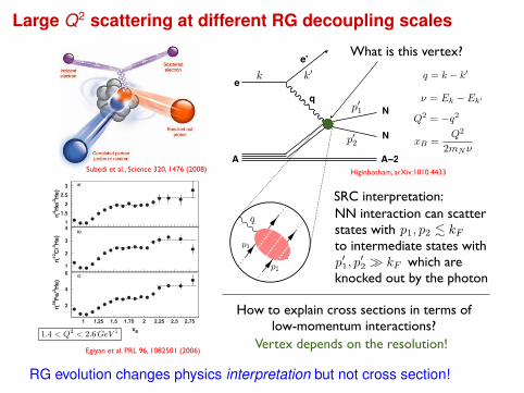
Subedi et al., Science 320, 1476 (2008)
would demonstrate the presence of 3-nucleon (3N) SRCand confirm the previous observation of NN SRC.
Note that: (i) Refs. [5,6] argue that the c.m. motion of theNN SRC may change the value of a2 (by up to 20% for56Fe) but not the scaling at xB < 2. For 3N SRC there areno estimates of the effects of c.m. motion. (ii) Final stateinteractions (FSI) are dominated by the interaction of thestruck nucleon with the other nucleons in the SRC [7,8].Hence the FSI can modify !j, while such modification ofaj!A" are small since the pp, pn, and nn cross sections atQ2 > 1 GeV2 are similar in magnitudes.
In our previous work [6] we showed that the ratiosR!A; 3He" # 3!A!Q2;xB"
A!3He!Q2;xB" scale for 1:5< xB < 2 and 1:4<
Q2 < 2:6 GeV2, confirming findings in Ref. [7]. Here werepeat our previous measurement with higher statisticswhich allows us to estimate the absolute per-nucleon prob-abilities of NN SRC.
We also search for the even more elusive 3N SRC,correlations which originate from both short-range NNinteractions and three-nucleon forces, using the ratioR!A; 3He" at 2< xB $ 3.
Two sets of measurements were performed at theThomas Jefferson National Accelerator Facility in 1999and 2002. The 1999 measurements used 4.461 GeV elec-trons incident on liquid 3He, 4He and solid 12C targets. The2002 measurements used 4.471 GeVelectrons incident on asolid 56Fe target and 4.703 GeV electrons incident on aliquid 3He target.
Scattered electrons were detected in the CLAS spec-trometer [9]. The lead-scintillator electromagnetic calo-rimeter provided the electron trigger and was used toidentify electrons in the analysis. Vertex cuts were usedto eliminate the target walls. The estimated remainingcontribution from the two Al 15 "m target cell windowsis less than 0.1%. Software fiducial cuts were used toexclude regions of nonuniform detector response. Kine-matic corrections were applied to compensate for driftchamber misalignments and magnetic field uncertainties.
We used the GEANT-based CLAS simulation, GSIM, todetermine the electron acceptance correction factors, tak-ing into account ‘‘bad’’ or ‘‘dead’’ hardware channels invarious components of CLAS. The measured acceptance-corrected, normalized inclusive electron yields on 3He,4He, 12C, and 56Fe at 1< xB < 2 agree with Sargsian’sradiated cross sections [10] that were tuned on SLAC data[11] and describe reasonably well the Jefferson Lab Hall C[12] data.
We constructed the ratios of inclusive cross sections as afunction of Q2 and xB, with corrections for the CLASacceptance and for the elementary electron-nucleon crosssections:
r!A; 3He" # A!2!ep % !en"3!Z!ep % N!en"
3Y!A"AY!3He"R
Arad; (2)
where Z and N are the number of protons and neutrons innucleus A, !eN is the electron-nucleon cross section, Y isthe normalized yield in a given (Q2; xB) bin, and RA
rad is theratio of the radiative correction factors for 3He and nucleusA [see Ref. [8] ]. In our Q2 range, the elementary crosssection correction factor A!2!ep%!en"
3!Z!ep%N!en" is 1:14& 0:02 for C
and 4He and 1:18& 0:02 for 56Fe. Note that the 3He yieldin Eq. (2) is also corrected for the beam energy differenceby the difference in the Mott cross sections. The corrected3He cross sections at the two energies agree within $ 3:5%[8].
We calculated the radiative correction factors for thereaction A!e; e0" at xB < 2 using Sargsian’s upgradedcode of Ref. [13] and the formalism of Mo and Tsai [14].These factors change 10%–15% with xB for 1< xB < 2.However, their ratios, RA
rad, for 3He to the other nuclei arealmost constant (within 2%–3%) for xB > 1:4. We appliedRArad in Eq. (2) event by event for 0:8< xB < 2. Since there
are no theoretical cross section calculations at xB > 2, weapplied the value of RA
rad averaged over 1:4< xB < 2 to theentire 2< xB < 3 range. Since the xB dependence of RA
radfor 4He and 12C are very small, this should not affect theratio r of Eq. (2). For 56Fe, due to the observed small slopeof RA
rad with xB, r!A; 3He" can increase up to 4% at xB #2:55. This was included in the systematic errors.
Figure 1 shows the resulting ratios integrated over 1:4<Q2 < 2:6 GeV2. These cross section ratios (a) scale ini-tially for 1:5< xB < 2, which indicates that NN SRCs
a)
r(4 H
e/3 H
e)
b)
r(12
C/3 H
e)
xB
r(56
Fe/3 H
e)
c)
1
1.5
2
2.5
3
1
2
3
4
2
4
6
1 1.25 1.5 1.75 2 2.25 2.5 2.75
FIG. 1. Weighted cross section ratios [see Eq. (2)] of (a) 4He,(b) 12C, and (c) 56Fe to 3He as a function of xB for Q2 >1:4 GeV2. The horizontal dashed lines indicate the NN (1:5<xB < 2) and 3N (xB > 2:25) scaling regions.
PRL 96, 082501 (2006) P H Y S I C A L R E V I E W L E T T E R S week ending3 MARCH 2006
082501-3
Higinbotham, arXiv:1010.4433
Egiyan et al. PRL 96, 1082501 (2006)
What is this vertex?
k k q = k − k
ν = Ek − Ek
p1
p2
p1
SRC interpretation:
NN interaction can scatter states withto intermediate states with which are knocked out by the photon
p1, p2 kF
How to explain cross sections in terms of low-momentum interactions?
Vertex depends on the resolution!
q
p1
p2
p1, p2 kF
p2
1.4 < Q2 < 2.6 GeV 2
Q2 = −q2
xB =Q2
2mNν
SRC explanation relies on high-momentum nucleons in structure
Large Q2 scattering at different RG decoupling scalesCorrelations in nuclear systems
A!1A
q
A
q
e e
e’ e’
a) b)
A!2
N
NN
FIGURE 1. The simple goal of short-range nucleon-nucleon correlation studies is to cleanly isolate diagram b) from a).Unfortunately, there are many other diagrams, including those with final-state interactions, that can produce the same final state asthe diagram scientists would like to isolate. If one could find kinematics that were dominated by diagram b) it would finally allowelectron scattering to provide new insights into the short-range part of the nucleon-nucleon potential.
For A(e,e’p) reactions, one can determine not only the energy and moment transferred, but also the energy and
momentum of the knocked-out nucleon. The difference between the transferred and detected energy and momentum
is referred to as the missing energy, Emiss and missing momentum, pmiss, respectively. From the theoretical works on
how short-range nucleon-nucleon correlations effects the momentum distribution of nucleons in the nucleus [6], it
is clear one must probe beyond the simple particle in an average potential motion of the nucleon in the nucleus of
approximately 250 MeV/c in order to observe the effects of correlations.
With the construction of the Jefferson Lab Continuous Electron Beam Facility (CEBAF) [7], it was possible to
do high-luminosity knock-out reactions in ideal quasi-elastic kinematics into the pmiss > 250 MeV/c region. In the
early Jefferson Lab knock-out reaction proposals, such as E89-044 3He(e,e’p)pn and 3He(e,e’p)d, these kinematics
were argued as the key to cleanly observe the effects of short-range correlations. And while final results of the
experiments were clearly effected by the presence of correlations, the magnitude of the cross sections in the high
missing momentum region was dominated by final-state interaction effects [8, 9]. Equally striking was the D(e,e’p)n
data from CLAS taken at Q2 > 5 [GeV/c]2 in xB < 1 kinematics [10]. Here it was shown that meson-exchange currents,final-state interaction, and delta-isobar configurations mask cleanly probing nucleon-nucleons even at extremely high
Q2 in xB < 1 kinematics.
NUCLEAR SCALING
With both the xB < 1 and xB = 1 kinematics practically ruled out for ever being able to cleanly probe short-range
correlations; there is only one region left to explore: xB > 1. This is a special region, since it is kinematically
forbidden for a free nucleon, and thus seems to be a natural place to observe effects of multi-nucleon interactions.
These kinematics were probed with limited statistics at SLAC [11] and the plateaus in the per nucleon ratios, r(A/d),
were claimed at to be evidence for short-range correlations [12].
In 2003, CLAS published high statics data in the same kinematic region. The results clearly showed that the plateaus
could only be seen for Q2 > 1 [GeV/c]2 and xB > 1 kinematics [13] as predicted by Frankfurt and Strikman [14]. But
plateaus alone are not evidence for correlations, just evidence that the functional form of the cross section is the same
for the two nuclei; so data was taken the xB > 2 region. By logic, if 1< xB < 2 is a region of two-nucleon correlations,
then the xB > 2 region should be dominated by three-nucleon correlations. The CLAS Q2 > 1 and xB > 2 experiment
reported observing a second scaling plateau as shown in Fig. 2 [15]. Preliminary results of Hall C high precision data
have shown roughly the same magnitude for these plateaus as CLAS and shown that there is no Q2 dependence in the
2< Q2 < 4 [GeV/c]2 range [16, 17].
Subedi et al., Science 320, 1476 (2008)
would demonstrate the presence of 3-nucleon (3N) SRCand confirm the previous observation of NN SRC.
Note that: (i) Refs. [5,6] argue that the c.m. motion of theNN SRC may change the value of a2 (by up to 20% for56Fe) but not the scaling at xB < 2. For 3N SRC there areno estimates of the effects of c.m. motion. (ii) Final stateinteractions (FSI) are dominated by the interaction of thestruck nucleon with the other nucleons in the SRC [7,8].Hence the FSI can modify !j, while such modification ofaj!A" are small since the pp, pn, and nn cross sections atQ2 > 1 GeV2 are similar in magnitudes.
In our previous work [6] we showed that the ratiosR!A; 3He" # 3!A!Q2;xB"
A!3He!Q2;xB" scale for 1:5< xB < 2 and 1:4<
Q2 < 2:6 GeV2, confirming findings in Ref. [7]. Here werepeat our previous measurement with higher statisticswhich allows us to estimate the absolute per-nucleon prob-abilities of NN SRC.
We also search for the even more elusive 3N SRC,correlations which originate from both short-range NNinteractions and three-nucleon forces, using the ratioR!A; 3He" at 2< xB $ 3.
Two sets of measurements were performed at theThomas Jefferson National Accelerator Facility in 1999and 2002. The 1999 measurements used 4.461 GeV elec-trons incident on liquid 3He, 4He and solid 12C targets. The2002 measurements used 4.471 GeVelectrons incident on asolid 56Fe target and 4.703 GeV electrons incident on aliquid 3He target.
Scattered electrons were detected in the CLAS spec-trometer [9]. The lead-scintillator electromagnetic calo-rimeter provided the electron trigger and was used toidentify electrons in the analysis. Vertex cuts were usedto eliminate the target walls. The estimated remainingcontribution from the two Al 15 "m target cell windowsis less than 0.1%. Software fiducial cuts were used toexclude regions of nonuniform detector response. Kine-matic corrections were applied to compensate for driftchamber misalignments and magnetic field uncertainties.
We used the GEANT-based CLAS simulation, GSIM, todetermine the electron acceptance correction factors, tak-ing into account ‘‘bad’’ or ‘‘dead’’ hardware channels invarious components of CLAS. The measured acceptance-corrected, normalized inclusive electron yields on 3He,4He, 12C, and 56Fe at 1< xB < 2 agree with Sargsian’sradiated cross sections [10] that were tuned on SLAC data[11] and describe reasonably well the Jefferson Lab Hall C[12] data.
We constructed the ratios of inclusive cross sections as afunction of Q2 and xB, with corrections for the CLASacceptance and for the elementary electron-nucleon crosssections:
r!A; 3He" # A!2!ep % !en"3!Z!ep % N!en"
3Y!A"AY!3He"R
Arad; (2)
where Z and N are the number of protons and neutrons innucleus A, !eN is the electron-nucleon cross section, Y isthe normalized yield in a given (Q2; xB) bin, and RA
rad is theratio of the radiative correction factors for 3He and nucleusA [see Ref. [8] ]. In our Q2 range, the elementary crosssection correction factor A!2!ep%!en"
3!Z!ep%N!en" is 1:14& 0:02 for C
and 4He and 1:18& 0:02 for 56Fe. Note that the 3He yieldin Eq. (2) is also corrected for the beam energy differenceby the difference in the Mott cross sections. The corrected3He cross sections at the two energies agree within $ 3:5%[8].
We calculated the radiative correction factors for thereaction A!e; e0" at xB < 2 using Sargsian’s upgradedcode of Ref. [13] and the formalism of Mo and Tsai [14].These factors change 10%–15% with xB for 1< xB < 2.However, their ratios, RA
rad, for 3He to the other nuclei arealmost constant (within 2%–3%) for xB > 1:4. We appliedRArad in Eq. (2) event by event for 0:8< xB < 2. Since there
are no theoretical cross section calculations at xB > 2, weapplied the value of RA
rad averaged over 1:4< xB < 2 to theentire 2< xB < 3 range. Since the xB dependence of RA
radfor 4He and 12C are very small, this should not affect theratio r of Eq. (2). For 56Fe, due to the observed small slopeof RA
rad with xB, r!A; 3He" can increase up to 4% at xB #2:55. This was included in the systematic errors.
Figure 1 shows the resulting ratios integrated over 1:4<Q2 < 2:6 GeV2. These cross section ratios (a) scale ini-tially for 1:5< xB < 2, which indicates that NN SRCs
a)
r(4 H
e/3 H
e)
b)
r(12
C/3 H
e)
xB
r(56
Fe/3 H
e)
c)
1
1.5
2
2.5
3
1
2
3
4
2
4
6
1 1.25 1.5 1.75 2 2.25 2.5 2.75
FIG. 1. Weighted cross section ratios [see Eq. (2)] of (a) 4He,(b) 12C, and (c) 56Fe to 3He as a function of xB for Q2 >1:4 GeV2. The horizontal dashed lines indicate the NN (1:5<xB < 2) and 3N (xB > 2:25) scaling regions.
PRL 96, 082501 (2006) P H Y S I C A L R E V I E W L E T T E R S week ending3 MARCH 2006
082501-3
Higinbotham, arXiv:1010.4433
Egiyan et al. PRL 96, 1082501 (2006)
What is this vertex?
k k q = k k
= Ek Ek
p1
p2
p1
SRC interpretation:
NN interaction can scatter states withto intermediate states with which are knocked out by the photon
p1, p2 kF
How to explain cross sections in terms of low-momentum interactions?
Vertex depends on the resolution!
q
p1
p2
p1, p2 kF
p2
1.4 < Q2 < 2.6 GeV 2
Q2 = q2
xB =Q2
2mN
RG evolution changes physics interpretation but not cross section!

Ab initio calculations: The nuclear structure hockey stick
Realis'c:BEswithin5%andstartsfromNN+3NFs
GauteHagen,DNP2016
Why has the reach of precision structure calculations increased?
Application of effective field theory (EFT) and renormalizationgroup (RG) methods =⇒ low-resolution (“softened”) potentialsExplosion of many-body methods: GFMC/AFDMC, (IT-)NCSM,coupled cluster, lattice EFT, IM-SRG, SCGF, UMOA, MBPT, . . .
Uses of the renormalization group (RG) [cf. S. Weinberg (1981)]
Improving perturbation theory; e.g., in QCD calculationsMismatch of energy scales can generate large logarithmsShift between couplings and loop integrals to reduce logs
Identifying universality in critical phenomenaFilter out short-distance degrees of freedom
Simplifying calculations of nuclear structure/reactionsMake nuclear physics look more like quantum chemistry!
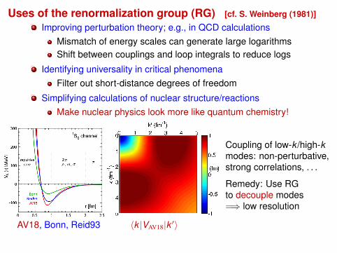
AV18, Bonn, Reid93 〈k |VAV18|k ′〉
Coupling of low-k /high-kmodes: non-perturbative,strong correlations, . . .
Remedy: Use RGto decouple modes=⇒ low resolution

Uses of the renormalization group (RG) [cf. S. Weinberg (1981)]
Improving perturbation theory; e.g., in QCD calculationsMismatch of energy scales can generate large logarithmsShift between couplings and loop integrals to reduce logs
Identifying universality in critical phenomenaFilter out short-distance degrees of freedom
Simplifying calculations of nuclear structure/reactionsMake nuclear physics look more like quantum chemistry!
“Vlow k ” Similarity RG
Vlow k : lower cutoff Λi in k , k ′
via dT (k , k ′; k2)/dΛ = 0
SRG: drive H toward diagonalwith flow equation
dHs/ds = [[Gs,Hs],Hs]
Continuous unitary transforms(cf. running couplings)

Uses of the renormalization group (RG) [cf. S. Weinberg (1981)]
Improving perturbation theory; e.g., in QCD calculationsMismatch of energy scales can generate large logarithmsShift between couplings and loop integrals to reduce logs
Identifying universality in critical phenomenaFilter out short-distance degrees of freedom
Simplifying calculations of nuclear structure/reactionsMake nuclear physics look more like quantum chemistry!
Block diagonal SRG Similarity RG
Vlow k : lower cutoff Λi in k , k ′
via dT (k , k ′; k2)/dΛ = 0
SRG: drive H toward diagonalwith flow equation
dHs/ds = [[Gs,Hs],Hs]
Continuous unitary transforms(cf. running couplings)

Uses of the renormalization group (RG) [cf. S. Weinberg (1981)]
Improving perturbation theory; e.g., in QCD calculationsMismatch of energy scales can generate large logarithmsShift between couplings and loop integrals to reduce logs
Identifying universality in critical phenomenaFilter out short-distance degrees of freedom
Simplifying calculations of nuclear structure/reactionsMake nuclear physics look more like quantum chemistry!
AV18:
Decoupling naturally visualized in momentum space for Gs = T
Phase-shift equivalent! Width of diagonal given by λ2 = 1/√
sWhat does this look like in coordinate space?

Uses of the renormalization group (RG) [cf. S. Weinberg (1981)]
Improving perturbation theory; e.g., in QCD calculationsMismatch of energy scales can generate large logarithmsShift between couplings and loop integrals to reduce logs
Identifying universality in critical phenomenaFilter out short-distance degrees of freedom
Simplifying calculations of nuclear structure/reactionsMake nuclear physics look more like quantum chemistry!
N3LO:(500 MeV)
Decoupling naturally visualized in momentum space for Gs = T
Phase-shift equivalent! Width of diagonal given by λ2 = 1/√
sWhat does this look like in coordinate space?

Visualizing the softening of NN interactionsProject non-local NN potential: Vλ(r) =
∫d3r ′ Vλ(r , r ′)
Roughly gives action of potential on long-wavelength nucleons
Central part (S-wave) [Note: The Vλ’s are all phase equivalent!]
Tensor part (S-D mixing) [graphs from K. Wendt et al., PRC (2012)]
=⇒ Flow to universal potentials!

Compare changing a cutoff in an EFT to RG decoupling(Local) field theory version in perturbation theory (diagrams)
Loops (sums over intermediate states)∆Λc⇐⇒ LECs
ddΛc
[︸ ︷︷ ︸∫ Λc d3q(2π)3
C0MC0k2−q2+iε
+ ︸ ︷︷ ︸C0(Λc)∝ Λc
2π2 +···
]= 0
Momentum-dependent vertices =⇒ Taylor expansion in k2
This implements an operator product expansion!
Claim: Vlow k RG and SRG decoupling work analogously“Vlow k ” SRG (“T” generator)

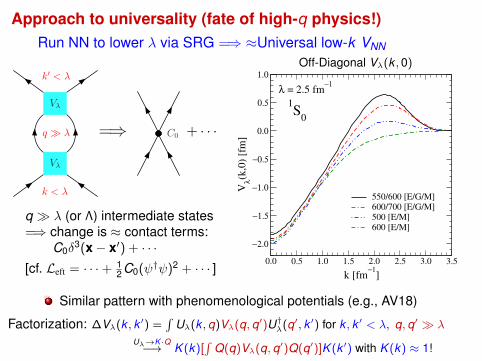
Approach to universality (fate of high-q physics!)Run NN to lower λ via SRG =⇒ ≈Universal low-k VNN
q ≫ λ
Vλ
Vλ
k < λ
k′ < λ
=⇒ C0 + · · ·
q λ (or Λ) intermediate states=⇒ change is ≈ contact terms:
C0δ3(x− x′) + · · ·
[cf. Left = · · ·+ 12 C0(ψ†ψ)2 + · · · ]
Off-Diagonal Vλ(k , 0)
0.0 0.5 1.0 1.5 2.0 2.5 3.0 3.5k [fm−1]
−2.0
−1.5
−1.0
−0.5
0.0
0.5
1.0
Vλ(k
,0) [
fm]
550/600 [E/G/M]600/700 [E/G/M]500 [E/M]600 [E/M]
λ = 5.0 fm−1
1S0
Similar pattern with phenomenological potentials (e.g., AV18)
Factorization: ∆Vλ(k , k ′) =∫
Uλ(k , q)Vλ(q, q′)U†λ(q′, k ′) for k , k ′ < λ, q, q′ λ
Uλ→K ·Q−→ K (k)[∫
Q(q)Vλ(q, q′)Q(q′)]K (k ′) with K (k) ≈ 1!

Approach to universality (fate of high-q physics!)Run NN to lower λ via SRG =⇒ ≈Universal low-k VNN
q ≫ λ
Vλ
Vλ
k < λ
k′ < λ
=⇒ C0 + · · ·
q λ (or Λ) intermediate states=⇒ change is ≈ contact terms:
C0δ3(x− x′) + · · ·
[cf. Left = · · ·+ 12 C0(ψ†ψ)2 + · · · ]
Off-Diagonal Vλ(k , 0)
0.0 0.5 1.0 1.5 2.0 2.5 3.0 3.5k [fm−1]
−2.0
−1.5
−1.0
−0.5
0.0
0.5
1.0
Vλ(k
,0) [
fm]
550/600 [E/G/M]600/700 [E/G/M]500 [E/M]600 [E/M]
λ = 4.0 fm−1
1S0
Similar pattern with phenomenological potentials (e.g., AV18)
Factorization: ∆Vλ(k , k ′) =∫
Uλ(k , q)Vλ(q, q′)U†λ(q′, k ′) for k , k ′ < λ, q, q′ λ
Uλ→K ·Q−→ K (k)[∫
Q(q)Vλ(q, q′)Q(q′)]K (k ′) with K (k) ≈ 1!

Approach to universality (fate of high-q physics!)Run NN to lower λ via SRG =⇒ ≈Universal low-k VNN
q ≫ λ
Vλ
Vλ
k < λ
k′ < λ
=⇒ C0 + · · ·
q λ (or Λ) intermediate states=⇒ change is ≈ contact terms:
C0δ3(x− x′) + · · ·
[cf. Left = · · ·+ 12 C0(ψ†ψ)2 + · · · ]
Off-Diagonal Vλ(k , 0)
0.0 0.5 1.0 1.5 2.0 2.5 3.0 3.5k [fm−1]
−2.0
−1.5
−1.0
−0.5
0.0
0.5
1.0
Vλ(k
,0) [
fm]
550/600 [E/G/M]600/700 [E/G/M]500 [E/M]600 [E/M]
λ = 3.0 fm−1
1S0
Similar pattern with phenomenological potentials (e.g., AV18)
Factorization: ∆Vλ(k , k ′) =∫
Uλ(k , q)Vλ(q, q′)U†λ(q′, k ′) for k , k ′ < λ, q, q′ λ
Uλ→K ·Q−→ K (k)[∫
Q(q)Vλ(q, q′)Q(q′)]K (k ′) with K (k) ≈ 1!
Approach to universality (fate of high-q physics!)Run NN to lower λ via SRG =⇒ ≈Universal low-k VNN
q ≫ λ
Vλ
Vλ
k < λ
k′ < λ
=⇒ C0 + · · ·
q λ (or Λ) intermediate states=⇒ change is ≈ contact terms:
C0δ3(x− x′) + · · ·
[cf. Left = · · ·+ 12 C0(ψ†ψ)2 + · · · ]
Off-Diagonal Vλ(k , 0)
0.0 0.5 1.0 1.5 2.0 2.5 3.0 3.5k [fm−1]
−2.0
−1.5
−1.0
−0.5
0.0
0.5
1.0
Vλ(k
,0) [
fm]
550/600 [E/G/M]600/700 [E/G/M]500 [E/M]600 [E/M]
λ = 2.5 fm−1
1S0
Similar pattern with phenomenological potentials (e.g., AV18)
Factorization: ∆Vλ(k , k ′) =∫
Uλ(k , q)Vλ(q, q′)U†λ(q′, k ′) for k , k ′ < λ, q, q′ λ
Uλ→K ·Q−→ K (k)[∫
Q(q)Vλ(q, q′)Q(q′)]K (k ′) with K (k) ≈ 1!

Approach to universality (fate of high-q physics!)Run NN to lower λ via SRG =⇒ ≈Universal low-k VNN
q ≫ λ
Vλ
Vλ
k < λ
k′ < λ
=⇒ C0 + · · ·
q λ (or Λ) intermediate states=⇒ change is ≈ contact terms:
C0δ3(x− x′) + · · ·
[cf. Left = · · ·+ 12 C0(ψ†ψ)2 + · · · ]
Off-Diagonal Vλ(k , 0)
0.0 0.5 1.0 1.5 2.0 2.5 3.0 3.5k [fm−1]
−2.0
−1.5
−1.0
−0.5
0.0
0.5
1.0
Vλ(k
,0) [
fm]
550/600 [E/G/M]600/700 [E/G/M]500 [E/M]600 [E/M]
λ = 2.0 fm−1
1S0
Similar pattern with phenomenological potentials (e.g., AV18)
Factorization: ∆Vλ(k , k ′) =∫
Uλ(k , q)Vλ(q, q′)U†λ(q′, k ′) for k , k ′ < λ, q, q′ λ
Uλ→K ·Q−→ K (k)[∫
Q(q)Vλ(q, q′)Q(q′)]K (k ′) with K (k) ≈ 1!

Approach to universality (fate of high-q physics!)Run NN to lower λ via SRG =⇒ ≈Universal low-k VNN
q ≫ λ
Vλ
Vλ
k < λ
k′ < λ
=⇒ C0 + · · ·
q λ (or Λ) intermediate states=⇒ change is ≈ contact terms:
C0δ3(x− x′) + · · ·
[cf. Left = · · ·+ 12 C0(ψ†ψ)2 + · · · ]
Off-Diagonal Vλ(k , 0)
0.0 0.5 1.0 1.5 2.0 2.5 3.0 3.5k [fm−1]
−2.0
−1.5
−1.0
−0.5
0.0
0.5
1.0
Vλ(k
,0) [
fm]
550/600 [E/G/M]600/700 [E/G/M]500 [E/M]600 [E/M]
λ = 1.5 fm−1
1S0
Similar pattern with phenomenological potentials (e.g., AV18)
Factorization: ∆Vλ(k , k ′) =∫
Uλ(k , q)Vλ(q, q′)U†λ(q′, k ′) for k , k ′ < λ, q, q′ λ
Uλ→K ·Q−→ K (k)[∫
Q(q)Vλ(q, q′)Q(q′)]K (k ′) with K (k) ≈ 1!
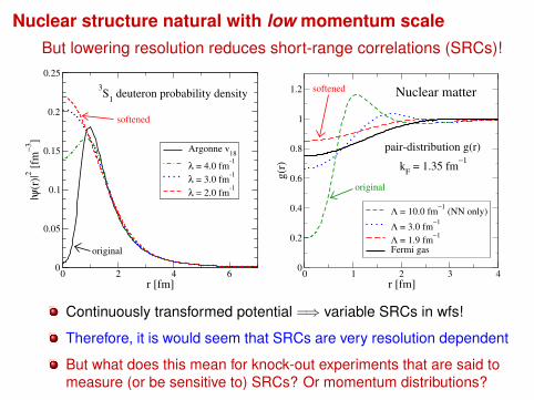
Nuclear structure natural with low momentum scaleBut lowering resolution reduces short-range correlations (SRCs)!
0 2 4 6r [fm]
0
0.05
0.1
0.15
0.2
0.25
|ψ(r
)|2 [
fm−
3]
Argonne v18
λ = 4.0 fm-1
λ = 3.0 fm-1
λ = 2.0 fm-1
3S
1 deuteron probability density
softened
original
0 1 2 3 4r [fm]
0
0.2
0.4
0.6
0.8
1
1.2
g(r
)
Λ = 10.0 fm−1
(NN only)
Λ = 3.0 fm−1
Λ = 1.9 fm−1
Fermi gas
pair-distribution g(r)
kF = 1.35 fm
−1
original
softened Nuclear matter
Continuously transformed potential =⇒ variable SRCs in wfs!
Therefore, it is would seem that SRCs are very resolution dependent
But what does this mean for knock-out experiments that are said tomeasure (or be sensitive to) SRCs? Or momentum distributions?

Deuteron scale-(in)dependent observables
0.51234510
Λ (fm−1
)
0
0.01
0.02
0.03
0.04
0.05
0.06
PD
−2.23
−2.225
−2.22
ED
0.02
0.025
0.03
ηsd
AV18
D-state probability
Asymptotic D-S ratio
Binding energy (MeV)
0.512345
Λ (fm−1
)
0
0.01
0.02
0.03
0.04
0.05
0.06
PD
−2.23
−2.225
−2.22
ED
0.02
0.025
0.03
ηsd
N3LO (500 MeV)
D-state probability
Asymptotic D-S ratio
Binding energy (MeV)
Vlow k RG transformations labeled by Λ (different VΛ’s)=⇒ soften interactions by lowering resolution (scale)=⇒ reduced short-range and tensor correlations
Energy and asymptotic D-S ratio are unchanged (cf. ANC’s)
But D-state probability changes (cf. spectroscopic factors)
What about other quantities and other nuclei?

Distribution of kinetic and potential energy in the deuteronLook at expectation value of kinetic and potential energies cut off at kmax
Ed (k < kmax) = Trel(k < kmax) + Vs(k < kmax)
=
∫ kmax
0dk∫ kmax
0dk′ ψ†d (k;λ)
(k2δ3(k− k′) + Vs(k,k′)
)ψd (k′;λ)
0 1 2 3 4 5
kmax
[fm−1]
−25
−20
−15
−10
−5
0
5
10
15
20
25
Ene
rgy
[MeV
]
⟨T⟩⟨V⟩sum
0 1 2 3 4 5
kmax
[fm−1]
0 1 2 3 4 5 6
kmax
[fm−1]
AV18 Vlow k
(Λ = 2 fm−1
)Vs (λ = 2 fm
−1)

Contributions to the ground-state energy
Look at ground-state matrix elements of KE, NN, 3N, 4N
1 2 3 4 5 10
λ
−50
−40
−30
−20
−10
0
10
20
30
40
g.s
. E
xpec
tati
on V
alue
(MeV
)
<Trel><V
NN>
<V3N
>
1 2 3 4 5 10
λ
−1
−0.5
0
3H
h- ω = 28
Nmax
= 18
Nmax
-A3 = 32
NN+NNN
1 2 3 4 5 10
λ
−100
−80
−60
−40
−20
0
20
40
60
80
g.s
. E
xp
ecta
tio
n V
alu
e (M
eV) <T
rel>
<VNN
>
<V3N
>
<V4N
>
1 2 3 4 5 10
λ
−4
−2
0
<Trel
>
<VNN
>
<V3N
>
<V4N
>
4He
h- ω = 28Nmax
= 18
Nmax
-A3 = 32
NN+NNN
Clear hierarchy, but also strong cancellations at NN level
What about the A dependence?
Kinetic energy is resolution dependent!

Parton vs. nuclear momentum distributions
From%Povh%et%al.,%Par$cles)and)Nuclei)
The quark distribution q(x ,Q2) isscale and scheme dependent
x q(x ,Q2) measures the share ofmomentum carried by the quarksin a particular x-interval
q(x ,Q2) and q(x ,Q20) are related
by RG evolution equations
0 1 2 3 4 5
5
10
1510!4
10!2
100
102
! (fm!1)
k (fm!1)
nd!(k
) (f
m3) SRCs%
No%SRCs%
Deuteron momentum distributionis scale and scheme dependent
Initial AV18 potential evolved withSRG from λ =∞ to λ = 1.5 fm−1
High momentum tail shrinks asλ decreases (lower resolution)

Factorization: high-E QCD vs. low-E nuclear
Parton distributions as paradigm [Marco Stratman]
July, 25-28 2005 PHENIX Spin Fest @ RIKEN Wako 20
!"#$%&'("$'%)*+#,-.-+
!"#$%&"'()&*!&*+*,$'$"%,)%-)-'#$%&".'$"%,/
,"&/*+#"0-
1"#$%&'("$'%)
-232
42*#0%"#*)%-) -5*/-1')-+*6%&/-&0')-*6-$7--)*0%)389+,%&$8/'+$")#-
:2*#0%"#*)%-)+#0*1*5*&-8+,;110')3*1')'$-*<'-#-+*
$,-*+-<"&"$'%) 6-$7--)*0%)38 ")/*+,%&$8/'+$")#-*<,=+'#+*'+*)%$*;)'>;-
+,%&$8/'+$")#-?'0+%)*#%-11'#'-)$
0%)38/'+$")#-<"&$%)*/-)+'$=
F2(x ,Q2) ∼∑a fa(x , µf )⊗ F a
2 (x ,Q/µf )
Parton distributions as paradigm [Marco Stratman]
July, 25-28 2005 PHENIX Spin Fest @ RIKEN Wako 20
!"#$%&'("$'%)*+#,-.-+
!"#$%&"'()&*!&*+*,$'$"%,)%-)-'#$%&".'$"%,/
,"&/*+#"0-
1"#$%&'("$'%)
-232
42*#0%"#*)%-) -5*/-1')-+*6%&/-&0')-*6-$7--)*0%)389+,%&$8/'+$")#-
:2*#0%"#*)%-)+#0*1*5*&-8+,;110')3*1')'$-*<'-#-+*
$,-*+-<"&"$'%) 6-$7--)*0%)38 ")/*+,%&$8/'+$")#-*<,=+'#+*'+*)%$*;)'>;-
+,%&$8/'+$")#-?'0+%)*#%-11'#'-)$
0%)38/'+$")#-<"&$%)*/-)+'$= ↔
Parton distributions as paradigm [Marco Stratman]
July, 25-28 2005 PHENIX Spin Fest @ RIKEN Wako 20
!"#$%&'("$'%)*+#,-.-+
!"#$%&"'()&*!&*+*,$'$"%,)%-)-'#$%&".'$"%,/
,"&/*+#"0-
1"#$%&'("$'%)
-232
42*#0%"#*)%-) -5*/-1')-+*6%&/-&0')-*6-$7--)*0%)389+,%&$8/'+$")#-
:2*#0%"#*)%-)+#0*1*5*&-8+,;110')3*1')'$-*<'-#-+*
$,-*+-<"&"$'%) 6-$7--)*0%)38 ")/*+,%&$8/'+$")#-*<,=+'#+*'+*)%$*;)'>;-
+,%&$8/'+$")#-?'0+%)*#%-11'#'-)$
0%)38/'+$")#-<"&$%)*/-)+'$=
Separation between long- andshort-distance physics is notunique =⇒ introduce µf
Choice of µf defines borderbetween long/short distance
Form factor F2 is independentof µf , but pieces are not
Q2 running of fa(x ,Q2) comesfrom choosing µf to optimizeextraction from experiment
Also has factorization assumptions(e.g., from D. Bazin ECT* talk, 5/2011)
D. Bazin, Workshop on Recent Developments in Transfer and Knockout Reactions, May 9-13, 2011, Trento, Italy
Conundrum
• Using reactions to study nuclear structure
• One observable, two models
• To extract structure information, need accurate reaction model
!if
=
!
|Jf!Ji|"j"Jf +Ji
Sifj !sp
Observable: cross section
Structure model: spectroscopic factor
Reaction model: single-particlecross section
Is the factorization general/robust?(Process dependence?)
What is the scale/schemedependence of extractedproperties?
What are the trade-offs? (Doessimpler structure always meanmuch more complicated reaction?)
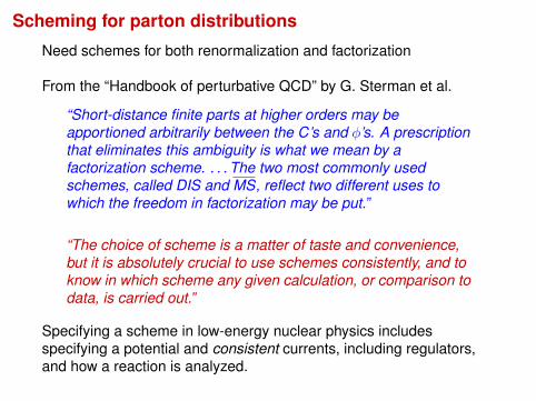
Scheming for parton distributions
Need schemes for both renormalization and factorization
From the “Handbook of perturbative QCD” by G. Sterman et al.
“Short-distance finite parts at higher orders may beapportioned arbitrarily between the C’s and φ’s. A prescriptionthat eliminates this ambiguity is what we mean by afactorization scheme. . . . The two most commonly usedschemes, called DIS and MS, reflect two different uses towhich the freedom in factorization may be put.”
“The choice of scheme is a matter of taste and convenience,but it is absolutely crucial to use schemes consistently, and toknow in which scheme any given calculation, or comparison todata, is carried out.”
Specifying a scheme in low-energy nuclear physics includesspecifying a potential and consistent currents, including regulators,and how a reaction is analyzed.

Source of scale-dependence for low-E structure
Measured cross section as convolution: reaction⊗structure
but separate parts are not unique, only the combination
Short-range unitary transformation U leaves m.e.’s invariant:
Omn ≡ 〈Ψm|O|Ψn〉 =(〈Ψm|U†
)UOU†
(U|Ψn〉
)= 〈Ψm|O|Ψn〉 ≡ Omn
Note: matrix elements of operator O itself between thetransformed states are in general modified:
Omn ≡ 〈Ψm|O|Ψn〉 6= Omn =⇒ e.g., 〈ΨA−1n |aα|ΨA
0 〉 changes
In a low-energy effective theory, transformations that modifyshort-range unresolved physics =⇒ equally valid states.So Omn 6= Omn =⇒ scale/scheme dependent observables.
RG unitary transformations change the decoupling scale =⇒change the factorization scale. Use to characterize and explorescale and scheme and process dependence!

All pieces mix with unitary transformation
A one-body current becomes many-body (cf. EFT current):
Uρ(q)U† = + α + · · ·
New wf correlations have appeared (or disappeared):
U|ΨA0 〉 = U
12C(e, e!p)X
1966 1988 2006
+ · · · =⇒ Z
12C(e, e!p)X
1966 1988 2006
+ α
12C(e, e!p)X
1966 1988 2006
+ · · ·
Similarly with |Ψf 〉 = a†p|ΨA−1n 〉
Thus spectroscopic factors are scale dependent
Final state interactions (FSI) are also modified by U
Bottom line: the cross section is unchanged only if all pieces areincluded, with the same U: H(λ), current operator, FSI, . . .
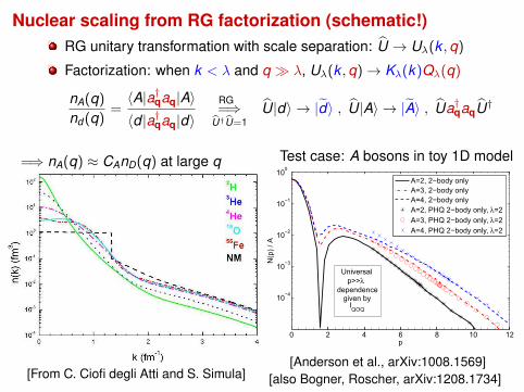
Nuclear scaling from RG factorization (schematic!)RG unitary transformation with scale separation: U → Uλ(k ,q)
Factorization: when k < λ and q λ, Uλ(k ,q)→ Kλ(k)Qλ(q)
nA(q)
nd (q)=〈A|a†qaq|A〉〈d |a†qaq|d〉
RG=⇒
U†U=1U|d〉 → |d〉 , U|A〉 → |A〉 , Ua†qaqU†
=⇒ nA(q) ≈ CAnD(q) at large q
nA(k) CA nD(k)
[From C. Ciofi degli Atti and S. Simula]
Test case: A bosons in toy 1D model
0 2 4 6 8 10 12
10−4
10−3
10−2
10−1
100
p
N(p
) / A
A=2, 2−body onlyA=3, 2−body onlyA=4, 2−body onlyA=2, PHQ 2−body only, λ=2A=3, PHQ 2−body only, λ=2A=4, PHQ 2−body only, λ=2
Universal p>>λdependence given by I
QOQ
[Anderson et al., arXiv:1008.1569][also Bogner, Roscher, arXiv:1208.1734]

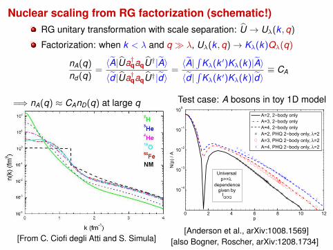
Nuclear scaling from RG factorization (schematic!)RG unitary transformation with scale separation: U → Uλ(k ,q)
Factorization: when k < λ and q λ, Uλ(k ,q)→ Kλ(k)Qλ(q)
nA(q)
nd (q)=〈A|Ua†qaqU†|A〉〈d |Ua†qaqU†|d〉
=〈A|∫
Uλ(k ′,q′)δq′qU†λ(q, k)|A〉〈d |∫
Uλ(k ′,q′)δq′qU†λ(q, k)|d〉
=⇒ nA(q) ≈ CAnD(q) at large q
nA(k) CA nD(k)
[From C. Ciofi degli Atti and S. Simula]
Test case: A bosons in toy 1D model
0 2 4 6 8 10 12
10−4
10−3
10−2
10−1
100
p
N(p
) / A
A=2, 2−body onlyA=3, 2−body onlyA=4, 2−body onlyA=2, PHQ 2−body only, λ=2A=3, PHQ 2−body only, λ=2A=4, PHQ 2−body only, λ=2
Universal p>>λdependence given by I
QOQ
[Anderson et al., arXiv:1008.1569][also Bogner, Roscher, arXiv:1208.1734]

Nuclear scaling from RG factorization (schematic!)RG unitary transformation with scale separation: U → Uλ(k ,q)
Factorization: when k < λ and q λ, Uλ(k ,q)→ Kλ(k)Qλ(q)
nA(q)
nd (q)=〈A|Ua†qaqU†|A〉〈d |Ua†qaqU†|d〉
=〈A|∫
Kλ(k ′)[∫
Qλ(q′)δq′qQλ(q)]Kλ(k)|A〉〈d |∫
Kλ(k ′)[∫
Qλ(q′)δq′qQλ(q)]Kλ(k)|d〉
=⇒ nA(q) ≈ CAnD(q) at large q
nA(k) CA nD(k)
[From C. Ciofi degli Atti and S. Simula]
Test case: A bosons in toy 1D model
0 2 4 6 8 10 12
10−4
10−3
10−2
10−1
100
p
N(p
) / A
A=2, 2−body onlyA=3, 2−body onlyA=4, 2−body onlyA=2, PHQ 2−body only, λ=2A=3, PHQ 2−body only, λ=2A=4, PHQ 2−body only, λ=2
Universal p>>λdependence given by I
QOQ
[Anderson et al., arXiv:1008.1569][also Bogner, Roscher, arXiv:1208.1734]
Nuclear scaling from RG factorization (schematic!)RG unitary transformation with scale separation: U → Uλ(k ,q)
Factorization: when k < λ and q λ, Uλ(k ,q)→ Kλ(k)Qλ(q)
nA(q)
nd (q)=〈A|Ua†qaqU†|A〉〈d |Ua†qaqU†|d〉
=〈A|∫
Kλ(k ′)Kλ(k)|A〉〈d |∫
Kλ(k ′)Kλ(k)|d〉≡ CA
=⇒ nA(q) ≈ CAnD(q) at large q
nA(k) CA nD(k)
[From C. Ciofi degli Atti and S. Simula]
Test case: A bosons in toy 1D model
0 2 4 6 8 10 12
10−4
10−3
10−2
10−1
100
p
N(p
) / A
A=2, 2−body onlyA=3, 2−body onlyA=4, 2−body onlyA=2, PHQ 2−body only, λ=2A=3, PHQ 2−body only, λ=2A=4, PHQ 2−body only, λ=2
Universal p>>λdependence given by I
QOQ
[Anderson et al., arXiv:1008.1569][also Bogner, Roscher, arXiv:1208.1734]

U-factorization with SRG [Anderson et al., arXiv:1008.1569]Factorization: Uλ(k ,q)→ Kλ(k)Qλ(q) when k < λ and q λ
Operator product expansion for nonrelativistic wf’s (see Lepage)
Ψ∞α (q) ≈ γλ(q)
∫ λ
0p2dp Z (λ)Ψλ
α(p) + ηλ(q)
∫ λ
0p2dp p2 Z (λ) Ψλ
α(p) + · · ·
Construct unitary transformation to get Uλ(k ,q) ≈ Kλ(k)Qλ(q)
Uλ(k , q) =∑α
〈k |ψλα〉〈ψ∞α |q〉 →
[αlow∑α
〈k |ψλα〉
∫ λ
0p2dp Z (λ)Ψλ
α(p)]γλ(q) + · · ·
Test of factorization of U:
Uλ(ki , q)
Uλ(k0, q)→ Kλ(ki )Qλ(q)
Kλ(k0)Qλ(q),
so for q λ⇒ Kλ(ki )Kλ(k0)
LO−→ 1
Look for plateaus: ki . 2 fm−1. q=⇒ it works!
Leading order =⇒ contact term! 0 1 2 3 4 5
q [fm−1
]
0.1
1
10
|U(k
i,q)
/ U
(k0,q
)|
k1 = 0.5 fm
−1
k2 = 1.0 fm
−1
k3 = 1.5 fm
−1
k4 = 3.0 fm
−1
λ = 2.0 fm−1
1S
0
k0 = 0.1 fm
−1

U-factorization with SRG [Anderson et al., arXiv:1008.1569]Factorization: Uλ(k ,q)→ Kλ(k)Qλ(q) when k < λ and q λ
Operator product expansion for nonrelativistic wf’s (see Lepage)
Ψ∞α (q) ≈ γλ(q)
∫ λ
0p2dp Z (λ)Ψλ
α(p) + ηλ(q)
∫ λ
0p2dp p2 Z (λ) Ψλ
α(p) + · · ·
Construct unitary transformation to get Uλ(k ,q) ≈ Kλ(k)Qλ(q)
Uλ(k , q) =∑α
〈k |ψλα〉〈ψ∞α |q〉 →
[αlow∑α
〈k |ψλα〉
∫ λ
0p2dp Z (λ)Ψλ
α(p)]γλ(q) + · · ·
Test of factorization of U:
Uλ(ki , q)
Uλ(k0, q)→ Kλ(ki )Qλ(q)
Kλ(k0)Qλ(q),
so for q λ⇒ Kλ(ki )Kλ(k0)
LO−→ 1
Look for plateaus: ki . 2 fm−1. q=⇒ it works!
Leading order =⇒ contact term! 0 1 2 3 4 5
q [fm−1
]
0.1
1
10
|U(k
i,q)
/ U
(k0,q
)|
k1 = 0.5 fm
−1
k2 = 1.0 fm
−1
k3 = 1.5 fm
−1
k4 = 3.0 fm
−1
λ = 2.0 fm−1
3S
1
k0 = 0.1 fm
−1

U-factorization with SRG [Anderson et al., arXiv:1008.1569]Factorization: Uλ(k ,q)→ Kλ(k)Qλ(q) when k < λ and q λ
Operator product expansion for nonrelativistic wf’s (see Lepage)
Ψ∞α (q) ≈ γλ(q)
∫ λ
0p2dp Z (λ)Ψλ
α(p) + ηλ(q)
∫ λ
0p2dp p2 Z (λ) Ψλ
α(p) + · · ·
Construct unitary transformation to get Uλ(k ,q) ≈ Kλ(k)Qλ(q)
Uλ(k , q) =∑α
〈k |ψλα〉〈ψ∞α |q〉 →
[αlow∑α
〈k |ψλα〉
∫ λ
0p2dp Z (λ)Ψλ
α(p)]γλ(q) + · · ·
Test of factorization of U:
Uλ(ki , q)
Uλ(k0, q)→ Kλ(ki )Qλ(q)
Kλ(k0)Qλ(q),
so for q λ⇒ Kλ(ki )Kλ(k0)
LO−→ 1
Look for plateaus: ki . 2 fm−1. q=⇒ it works!
Leading order =⇒ contact term! 0 1 2 3 4 5
q [fm−1
]
0.1
1
10
|U(k
i,q)
/ U
(k0,q
)| *
(k
0/k
i)
k1 = 0.5 fm
−1
k2 = 1.0 fm
−1
k3 = 1.5 fm
−1
k4 = 3.0 fm
−1
λ = 2.0 fm−1
1P
1
k0 = 0.3 fm
−1

How should one choose a scale and/or scheme?
To make calculations easier or more convergentQCD running coupling and scale: improved perturbationtheory; choosing a gauge: e.g., Coulomb or LorentzLow-k potential: improve many-body convergence,
or to make microscopic connection to shell model or . . .(Near-) local potential: quantum Monte Carlo methods work
Better interpretation or intuition =⇒ predictabilitySRC phenomenology?
Cleanest extraction from experimentCan one “optimize” validity of impulse approximation?Ideally extract at one scale, evolve to others using RG
Plan: use range of scales to test calculations and physicsFind (match) Hamiltonians and operators with EFTUse renormalization group to consistently relate scales andquantitatively probe ambiguities (e.g., in spectroscopic factors)

Summary: Precision nuclear structure and reactions
We’re in a golden age for low-energy nuclear physicsMany complementary methods able to incorporate 3NFsSynergies of theory and experimentLarge-scale collaborations facilitate progressMany opportunities and challenges for precision physics
EFT and RG have become important tools for precisionRobust uncertainty quantification is a frontierScale and scheme dependence is inevitable =⇒ deal with it!
Challenges for which EFT/RG perspective + tools can helpCan we have controlled factorization at low energies?How should one choose a scale/scheme in particular cases?What is the scheme-dependence of SF’s and other quantities?What are the roles of short-range/long-range correlations?How do we consistently match Hamiltonians and operators?. . . and many more. Calculations are in progress!

Backups

EMC effect from the EFT perspective
Exploit scale separation between short- and long-distance physics
Match complete set of operator matrix elements (power count!)Cf. needing a model of short-distance nucleon dynamicsDistinguish long-distance nuclear from nucleon physics
EMC and effective field theory (examples)
“DVCS-dissociation of the deuteron and the EMC effect”[S.R. Beane and M.J. Savage, Nucl. Phys. A 761, 259 (2005)]
“By constructing all the operators required to reproduce the matrixelements of the twist-2 operators in multi-nucleon systems, one seesthat operators involving more than one nucleon are not forbidden by thesymmetries of the strong interaction, and therefore must be present.While observation of the EMC effect twenty years ago may have beensurprising to some, in fact, its absence would have been far moresurprising.”
“Universality of the EMC Effect”[J.-W. Chen and W. Detmold, Phys. Lett. B 625, 165 (2005)]
“SRCs and the EMC Effect in EFT” [Chen et al., arXiv:1607.03065]

A dependence of the EMC effect is long-distance physics!EFT treatment by Chen and Detmold [Phys. Lett. B 625, 165 (2005)]
F A2 (x) =
∑i
Q2i xqA
i (x) =⇒ RA(x) = F A2 (x)/AF N
2 (x)
“The x dependence of RA(x) is governed by short-distancephysics, while the overall magnitude (the A dependence) ofthe EMC effect is governed by long distance matrix elementscalculable using traditional nuclear physics.”
Match matrix elements: leading-order nucleon operators toisoscalar twist-two quark operators
J.-W. Chen, W. Detmold / Physics Letters B 625 (2005) 165–170 167
symmetries [14–17]. The leading one- and two-bodyhadronic operators in the matching are
(4)Oµ0···µn
q =!xn
"qvµ0 · · ·vµnN†N
#1+ !nN
†N$+ · · · ,
where vµ = vµ + O(1/M) is the velocity of thenucleus. Operators involving additional derivativesare suppressed by powers of M in the EFT power-counting. In Eq. (4) we have only kept the SU(4) (spinand isospin) singlet two-body operator !nv
µ0 · · ·!vµn(N†N)2. The other independent two-body oper-ator "nv
µ0 · · ·vµn(N†!N)2, which is non-singlet inSU(4) (! is an isospin matrix), is neglected because"n/!n = O(1/N2
c ) " 0.1 [21], where Nc is the num-ber of colors. Furthermore, the matrix element of(N†!N)2 for an isoscalar state with atomic num-ber A is smaller than that of (N†N)2 by a factor A
[10]. Three- and higher-body operators also appear inEq. (4); numerical evidence from other EFT calcula-tions indicates that these contributions are generallymuch smaller than two-body ones [22].Nuclear matrix elements of Oµ0···µn
q give the mo-ments of the isoscalar nuclear parton distributions,qA(x). The leading order (LO) and the next-to-leadingorder (NLO) contributions to these matrix elementsare shown in Fig. 1(a) and (b), respectively. For an un-polarised, isoscalar nucleus,
!xn
"q|A # vµ0 · · ·vµn$A|Oµ0···µn
q |A%
(5)=!xn
"q
#A + $A|!n
%N†N
&2|A%$,
where we have used $A|N†N |A% = A. Notice that ifthere were no EMC effect, the !n would vanish forall n. Also !0 = 0 because of charge conservation. As-ymptotic relations [23] and analysis of experimentaldata [2,24] suggests that !1 " 0, implying that quarkscarry very similar fractions of a nucleon’ and a nucle-us’ momentum though no symmetry guarantees this.From Eq. (5) we see that the ratio
(6)$xn%q|AA$xn%q & 1$xm%q|AA$xm%q & 1
= !n
!m
is independent ofAwhich has powerful consequences.In all generality, the isoscalar nuclear quark distribu-tion can be written as
(7)qA(x) = A#q(x) + g(x,A)
$.
Taking moments of Eq. (7), Eq. (6) then demands thatthe x dependence and A dependence of g factorise,
(8)g(x,A) = g(x)G(A),
with
(9)G(A) = $A|%N†N
&2|A%/A#30,
and g(x) satisfying
(10)!n = 1#30$xn%q
A'
&A
dx xng(x).
#0 is an arbitrary dimensionful parameter and will bechosen as #0 = 1 fm&1. Crossing symmetry dictates
Fig. 1. Contributions to nuclear matrix elements. The dark square represents the various operators in Eq. (4) and the light shaded ellipsecorresponds to the nucleus, A. The dots in the lower part of the diagram indicate the spectator nucleons.
=⇒ 〈x2〉qvµ0 · · · vµn N†N[1 + αnN†N] + · · ·
RA(x) =F A
2 (x)
AF N2 (x)
= 1+gF2 (x)G(A) where G(A) = 〈A|(N†N)2|A〉/AΛ0
=⇒ the slope dRAdx scales with G(A) [Why is this not cited more?]

Scaling and EMC correlation via low resolution
SRG factorization, e.g.,Uλ(k ,q)→ Kλ(k)Qλ(q)when k < λ and q λ
Dependence on high-qindependent of A=⇒ universal [cf. Neff et al.]
A dependence fromlow-momentum matrixelements =⇒ calculate!
EMC from EFT using OPE:
Isolate A dependence, whichfactorizes from xEMC A dependence fromlong-distance matrix elements
Short Range Correlations and the EMC e!ect
Deep inelastic scattering ratio atQ2 ! 2GeV2 and 0.35 " xB " 0.7and inelastic scattering atQ2 ! 1.4GeV2 and 1.5 " xB " 2.0
Strong linear correlation betweenslope of ratio of DIS cross sections(nucleus A vs. deuterium) andnuclear scaling ratio
SRG Factorization at leading order:# Dependence on high-q
is independent of A# A-dependence from low
momentum matrix elementindependent of operator
L.B. Weinstein, et al., Phys. Rev. Lett. 106, 052301 (2011)
Why should A-dependence of nuclear scaling a2 and the EMC e!ect bethe same?
Overview Operators Factorization Conclusions Principles Applications
If the same leading operators dominate, then does linear Adependence of ratios follow immediately?Need to do quantitative calculations to explore!

What about long-range correlations?
SF calculations with FRPAChiral N3LO Hamiltonian
Soft =⇒ small SRCSRC contribution to SF changesdramatically with lower resolution
Compare short-range correlations(SRC) to long-range correlationsfrom particle-vibration coupling
LRC SRC!!
How scale/scheme dependentare long-range correlations?
Additional microscopiccalculations are needed!
C. Barbieri, PRL 103 (2009)
g!r; r0;!" #X
n
!c A$1n !r""%c A$1
n !r0"!& !EA$1
n & EA0 " $ i!
$X
k
c A&1k !r"!c A&1
k !r0""%!$ !EA&1
k & EA0 " & i!
; (2)
where the residues are the overlap amplitudes (1) and thepoles give experimental energy transfers. These refer tonucleon pickup (knockout) to the excited states of thesystems with A$ 1 (A& 1) particles. The propagator (2)is obtained by solving the Dyson equation [g!!" #g!0"!!" $ g!0"!!"!?!!"g!!"], where g!0"!!" propagatesa free nucleon. The information on nuclear structure isincluded in the irreducible self-energy, which was splitinto two contributions:
!?!r; r0;!" # !MF!r; r0;!" $ ~!!r; r0;!": (3)
The term !MF!!" includes both the nuclear mean field(MF) and diagrams describing two-particle scattering out-side the model space, generated using a G-matrix resum-mation [24]. As a consequence, it acquires an energydependence which is induced by SRC among nucleons
[23]. The second term, ~!!!", includes the LRC. In the
present work, ~!!!" is calculated in the so-called Faddeevrandom phase approximation (FRPA) of Refs. [21,25].This includes diagrams for particle-vibration coupling atall orders and with all possible vibration modes, see Fig. 1,as well as low-energy 2p1h=2h1p configurations. Particle-vibration couplings play an important role in compressingthe single-particle spectrum at the Fermi energy to itsexperimental density. However, a complete configurationmixing of states around the Fermi surface is still missingand would require SM calculations.
Each spectroscopic amplitude c A'1!r" appearing inEq. (2) has to be normalized to its respective SF as
Z" #Z
drjc A'1" !r"j2 # 1
1& @!?" "!!"@!
!!!!!!!!!#'!EA'1" &EA
0 "; (4)
where !?" "!!" ( hc "j!?!!"jc "i is the matrix element
of the self-energy calculated for the overlap function itselfbut normalized to unity (
Rdrjc "!r"j2 # 1). By inserting
Eq. (3) into (4), one distinguishes two contributions to thequenching of SFs. For model spaces sufficiently large, all
low-energy physics is described by ~!!!". Then, the de-rivative of !MF!!" accounts for the coupling to statesoutside the model space and estimates the effects of SRCalone [26].In general, the self-consistent (SC) self-energy (3) is a
functional of the one-body propagator itself, !? # !?)g*.Hence, the FRPA equations for the self-energy and theDyson equation have to be solved iteratively. The mean-field part, !MF)g*, was calculated exactly in terms of thefully fragmented propagator (2). For the FRPA, this pro-
cedure was simplified by employing the ~!)gIPM* obtainedin terms of a MF-like propagator
gIPM!r; r0;!" #X
n=2F
!#n!r""%#n!r0"!& "IMP
n $ i!
$X
k2F
#k!r"!#k!r0""%!& "IMP
k & i!; (5)
FIG. 1 (color online). Left. One of the diagrams included in
the correlated self-energy, ~!!!". Arrows up (down) refer toquasiparticle (quasihole) states, the "!ph" propagators includecollective ph and charge-exchange resonances, and the gII in-clude pairing between two particles or two holes. The FRPAmethod sums analogous diagrams, with any numbers of pho-nons, to all orders [21,25]. Right. Single-particle spectral distri-bution for neutrons in 56Ni, obtained from FRPA. Energies above(below) EF are for transitions to excited states of 57Ni (55Ni).The quasiparticle states close to the Fermi surface are clearlyvisible. Integrating over r [Eq. (4)] gives the SFs reported inTable I.
TABLE I. Spectroscopic factors (given as a fraction of theIPM) for valence orbits around 56Ni. For the SC FRPA calcu-lation in the large harmonic oscillator space, the values shownare obtained by including only SRC, SRC and LRC fromparticle-vibration couplings (full FRPA), and by SRC, particle-vibration couplings and extra correlations due to configurationmixing (FRPA$#Z"). The last three columns give the resultsof SC FRPA and SM in the restricted 1p0f model space. The#Z"s are the differences between the last two results and aretaken as corrections for the SM correlations that are not alreadyincluded in the FRPA formalism.
10 osc. shells Exp. [29] 1p0f spaceFRPA(SRC)
FullFRPA
FRPA$#Z" FRPA SM #Z"
57Ni:$1p1=2 0.96 0.63 0.61 0.79 0.77 &0:02$0f5=2 0.95 0.59 0.55 0.79 0.75 &0:04$1p3=2 0.95 0.65 0.62 0.58(11) 0.82 0.79 &0:03
55Ni:$0f7=2 0.95 0.72 0.69 0.89 0.86 &0:03
57Cu:%1p1=2 0.96 0.66 0.62 0.80 0.76 &0:04%0f5=2 0.96 0.60 0.58 0.80 0.78 &0:02%1p3=2 0.96 0.67 0.65 0.81 0.79 &0:02
55Co:%0f7=2 0.95 0.73 0.71 0.89 0.87 &0:02
PRL 103, 202502 (2009) P HY S I CA L R EV I EW LE T T E R Sweek ending
13 NOVEMBER 2009
202502-2

What can we say about the flow of NN· · ·N potentials?Can arise from counterterm for new UV cutoff dependence,e.g., changes in Λc must be absorbed by 3-body coupling D0(Λc)
ddΛc
[+︸ ︷︷ ︸
∝(C0)4 ln(k/Λc)
+ ︸ ︷︷ ︸D0(Λc)∝(C0)4 ln(a0Λc)
]= 0
RG invariance dictates 3-body coupling flow [Braaten & Nieto]
General RG: 3NF from integrating out or decoupling high-k states
π, ρ, ω∆, N∗
π, ρ, ω
π, ρ, ω
π, ρ, ω
N
low⇓ resolution
π π π
c1, c3, c4 cD cE

Is there 3NF universality?
Evolve chiral NNLO EFT potentials in momentum plane wave basisto λ = 1.5 fm−1 [K. Hebeler, Phys. Rev. C85 (2012) 021002]
In one 3-body partial wave, fix one Jacobi momentum (p,q)and plot vs. the other one:
0 1 2 3p [fm
−1]
-0.02
0
0.02
0.04
0.06
0.08
0.1
<p
q α
| V12
3 | p
q α
> [
fm4 ]
450/500 MeV600/500 MeV550/600 MeV450/700 MeV600/700 MeV
0 1 2 3 4q [fm
−1]
q = 1.5 fm−1
p = 0.75 fm−1
Collapse of curves includes non-trivial structure

Is there 3NF universality?
Evolve in discretized momentum-space hyperspherical harmonicsbasis to λ = 1.4 fm−1 [K. Wendt, Phys. Rev. C87 (2013) 061001]
Contour plot of integrand for 3NF expectation value in triton
Local projections of 3NF also show flow toward universal form
Can we exploit universality a la Wilson? Stay tuned!

Nuclear structure natural with low momentum scaleSoftened potentials (SRG, Vlow k , UCOM, . . . ) enhance convergence
Convergence for no-core shellmodel (NCSM):
(Already) soft chiral EFT potentialand evolved (softened) SRGpotentials, including NNN
Softening allows importancetruncation (IT) and convergedcoupled cluster (CCSD)
-130
-120
-110
-100
-90
.
E[M
eV
]
NN+3N-ind.
16O
IT-NCSM
NN+3N-ind.
~Ω = 20 MeV
CCSD
2 4 6 8 10 12 14 16 18Nmax
-150
-140
-130
-120
.
E[M
eV
]
NN+3N-full
16 14 12 10 8 6 4 2emax
NN+3N-full
[Roth et al., PRL 109, 052501 (2012)]
Also enables ab initio nuclear reactions with NCSM/RGM [Navratil et al.]

Nuclear structure natural with low momentum scaleTeam Roth: SRG-evolved N3LO with NNN [PRL 109, 052501 (2012)]
Coupled cluster with interactions H(λ): λ is a decoupling scaleOnly when NNN-induced added to NN-only =⇒ λ independent
With initial NNN: predictions from fit only to A = 3 properties
Open questions: red (400 MeV) works, blue (500 MeV) doesn’t!
-170
-160
-150
-140
-130
-120
-110
-100
.
E[M
eV]
NN-only
exp.
NN+3N-ind.
16O!! = 20 MeV
NN+3N-full
2 4 6 8 10 12 14emax
-240
-220
-200
-180
-160
-140
-120
.
E[M
eV] exp.
2 4 6 8 10 12 14emax
24O!! = 20 MeV
2 4 6 8 10 12 14emax
-600
-550
-500
-450
-400
-350
-300
-250
.
E[M
eV]
NN-only
exp.
NN+3N-ind.
40Ca!! = 20 MeV
NN+3N-full
2 4 6 8 10 12 14emax
-800
-700
-600
-500
-400
-300
.
E[M
eV]
exp.
2 4 6 8 10 12 14emax
48Ca!! = 20 MeV
2 4 6 8 10 12 14emax
Same predictions for λ’s! (issues about NNN resolved by 4N?)
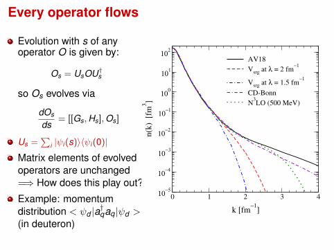
Every operator flows
Evolution with s of anyoperator O is given by:
Os = UsOU†s
so Os evolves via
dOs
ds= [[Gs,Hs],Os]
Us =∑
i |ψi (s)〉〈ψi (0)|Matrix elements of evolvedoperators are unchanged=⇒ How does this play out?
Example: momentumdistribution < ψd |a†qaq|ψd >(in deuteron)
0 1 2 3 4
k [fm−1
]
10−5
10−4
10−3
10−2
10−1
100
101
102
n(k
) [
fm3]
AV18
Vsrg at λ = 2 fm−1
Vsrg at λ = 1.5 fm−1
CD-Bonn
N3LO (500 MeV)

Flow equations lead to many-body operatorsConsider a’s and a†’s wrt s.p. basis and reference state:
dVs
ds=[[∑
a†a︸︷︷︸Gs
,∑
a†a†aa︸ ︷︷ ︸2-body
],∑
a†a†aa︸ ︷︷ ︸2-body
]= · · ·+
∑a†a†a†aaa︸ ︷︷ ︸
3-body!
+ · · ·
so there will be A-body forces (and operators) generatedIs this a problem?
Ok if “induced” many-body forces are same size as naturalonesAlternative: choose a non-vacuum reference state [Scott]
Nuclear 3-body forces already needed in unevolvedpotential
In fact, there are A-body forces (operators) initiallyNatural hierarchy from chiral EFT
=⇒ stop flow equations before unnatural 3-body sizeMany-body methods must deal with them!
SRG is a tractable method to evolve many-body operators

Observations on three-body forces
Three-body forces arise fromeliminating/decoupling dof’s
excited states of nucleonrelativistic effectshigh-momentumintermediate states
Omitting 3-body forces leadsto model dependence
observables depend on Λ/λ
cutoff dependence as tool
NNN at different Λ/λ can beevolved or fit to χEFT
how large is 4-body?
saturation of nuclear matter(K. Hebeler — corrected +improved 3NF treatment)
π, ρ, ω∆, N∗
π, ρ, ω
π, ρ, ω
π, ρ, ω
N
7.6 7.8 8 8.2 8.4 8.6 8.8Eb(
3H) [MeV]
24
25
26
27
28
29
30
31
E b(4 He)
[MeV
]
NN potentialsSRG N3LO (500 MeV)
N3LOλ=1.0
λ=3.0λ=1.25 λ=2.5
λ=2.25λ=1.5 λ=2.0
λ=1.75
Expt.
A=3,4 binding energiesSRG NN only, λ in fm−1

Observations on three-body forces
Three-body forces arise fromeliminating/decoupling dof’s
excited states of nucleonrelativistic effectshigh-momentumintermediate states
Omitting 3-body forces leadsto model dependence
observables depend on Λ/λ
cutoff dependence as tool
NNN at different Λ/λ can beevolved or fit to χEFT
how large is 4-body?saturation of nuclear matter(K. Hebeler — corrected +improved 3NF treatment)
π π π
c1, c3, c4 cD cE
0.8 1.0 1.2 1.4 1.6
kF [fm
−1]
−30
−25
−20
−15
−10
−5
0
Ener
gy/n
ucl
eon [
MeV
]
Λ = 1.8 fm−1
Λ = 2.8 fm−1
Λ = 1.8 fm−1
NN only
Λ = 2.8 fm−1
NN only
Vlow k
NN from N3LO (500 MeV)
3NF fit to E3H and r4He
Λ3NF
= 2.0 fm−1
3rd order pp+hh
NN + 3N
NN only

Tjon line revisited
7.6 7.8 8 8.2 8.4 8.6 8.8
Eb(3H) [MeV]
24
25
26
27
28
29
30
Eb(4
He)
[M
eV]
Tjon line for NN-only potentials
SRG NN-only
SRG NN+NNN (λ >1.7 fm−1
)
8.45 8.528.2
28.3
28.4
N3LO
λ=3.0λ=1.2
λ=2.5
λ=1.5
λ=2.0
λ=1.8
Expt.
(500 MeV)

Every operator flows [see Anderson et al., arXiv:1008.1569]
Evolution with s of anyoperator O is given by:
Os = UsOU†s
so Os evolves via
dOs
ds= [[Gs,Hs],Os]
Us =∑
i |ψi (s)〉〈ψi (0)|Matrix elements of evolvedoperators are unchanged
Consider momentumdistribution < ψd |a†qaq|ψd >
at q = 0.34 and 3.0 fm−1
0 1 2 3 4
q [fm−1]
10-5
10-4
10-3
10-2
10-1
100
101
102
4π [u
(q)2 +
w(q
)2 ] [fm
3 ]
N3LO unevolvedλ = 2.0 fm−1
λ = 1.5 fm−1
(a
qaq) deuteron

High and low momentum operators in deuteronIntegrand of (Ua†qaqU†) for q = 0.34 fm−1
Integrand for q = 3.02 fm−1
Momentumdistribution
0 1 2 3 4
q [fm−1]
10-5
10-4
10-3
10-2
10-1
100
101
102
4π [u
(q)2 +
w(q
)2 ] [fm
3 ]
N3LO unevolvedλ = 2.0 fm−1
λ = 1.5 fm−1
(a
qaq) deuteron
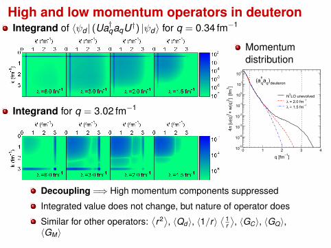
Decoupling =⇒ High momentum components suppressed
Integrated value does not change, but nature of operator does
Similar for other operators:⟨r2⟩, 〈Qd 〉, 〈1/r〉
⟨ 1r
⟩, 〈GC〉, 〈GQ〉,
〈GM〉

High and low momentum operators in deuteronIntegrand of 〈ψd | (Ua†qaqU†) |ψd〉 for q = 0.34 fm−1
Integrand for q = 3.02 fm−1
Momentumdistribution
0 1 2 3 4
q [fm−1]
10-5
10-4
10-3
10-2
10-1
100
101
102
4π [u
(q)2 +
w(q
)2 ] [fm
3 ]
N3LO unevolvedλ = 2.0 fm−1
λ = 1.5 fm−1
(a
qaq) deuteron
Decoupling =⇒ High momentum components suppressed
Integrated value does not change, but nature of operator does
Similar for other operators:⟨r2⟩, 〈Qd 〉, 〈1/r〉
⟨ 1r
⟩, 〈GC〉, 〈GQ〉,
〈GM〉
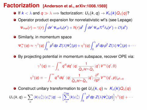
Factorization [Anderson et al., arXiv:1008.1569]
If k < λ and q λ =⇒ factorization: Uλ(k ,q)→ Kλ(k)Qλ(q)?
Operator product expansion for nonrelativistic wf’s (see Lepage)
Ψtrue(r) = γ(r)
∫dr ′Ψeff δa(r ′) + n(r)a2
∫dr ′Ψeff∇2δa(r ′) +O(a4)
Similarly, in momentum space
Ψ∞α (q) ≈ γλ(q)
∫ λ
0p2dp Z (λ)Ψλ
α(p) + ηλ(q)
∫ λ
0p2dp p2 Z (λ) Ψλ
α(p) + · · ·
By projecting potential in momentum subspace, recover OPE via:
γλ(q) ≡ −∫ ∞λ
q′2dq′ 〈q| 1
QλH∞Qλ
|q′〉V∞(q′, 0)
ηλ(q) ≡ −∫ ∞λ
q′2dq′ 〈q| 1
QλH∞Qλ
|q′〉 ∂2
∂p2 V∞(q′, p)|p2=0
Construct unitary transformation to get Uλ(k ,q) ≈ Kλ(k)Qλ(q)
Uλ(k , q) =∑α
〈k |ψλα〉〈ψ∞α |q〉 →
[αlow∑α
〈k |ψλα〉
∫ λ
0p2dp Z (λ)Ψλ
α(p)]γλ(q) + · · ·

Impact of VNN “collapse” on A ≥ 3 observables
Limited cases so far and NN-only: [K. Hebeler, E. Jurgenson]
0.8 1.0 1.2 1.4 1.6
kF [fm
−1]
0
5
10
15
20
Sp
read
[M
eV]
bare NN Λ = 2.0 fm
-1
λ = 2.0 fm-1
−40
−30
−20
−10
0
En
erg
y/n
ucl
eon
[M
eV]
EGM 550/600 MeVEGM 600/700 MeVEM 500 MeVEM 600 MeV
NN-only
1 2 3 4 5 10
λ [fm−1
]
−8.5
−8
−7.5
−7
−6.5
Gro
un
d-S
tate
En
erg
y [
MeV
]
AV18 (36/44)
CD-Bonn (32/44)
N3LO (32/28)
3H
NN-only
Exp
Nuclear matter spread (Vlow k shown) sizable at λ ≈ 2 fm−1
Binding energy collapse in light nuclei only for λ ≤ 1.5 fm−1