Abstract—We provide a method to specify location based

spectrum rights that enables spectrum management with finer resolution in space and frequency. This method accounts for the attenuation of transmissions from their source and so reveals the location based opportunities to reuse spectrum. The method uses a concise yet flexible data structure that has six parts: a signal strength, a frequency, a spectrum mask, a power map, a propagation map, and a scaling factor. Through the use of one or multiple of these parts most any type of spatial spectrum use authorization or protection may be defined. The structure allows spectrum to be managed as a spatial resource and so subdivided for spatial reuse or for resale. We provide several examples to demonstrate its versatility in spectrum management. We provide some observations and theorems that are useful in developing algorithms to verify compliance to the rights and restrictions conveyed in the proposed method and to discern when coexistent spectrum use is possible. This method provides a unified approach to define spectrum use that can be used to license spectrum, to optimize spectrum reuse, to negotiate spectrum rights, and to specify spectrum policy. It is ideally suited for over-the-air management of spectrum use.

Index Terms—Dynamic spectrum access networks, spectrum rights, spectrum regulation, propagation maps, power maps, fast command and control spectrum management model.

I. INTRODUCTION T is envisioned that a next generation set of wireless communications devices will dynamically access spectrum,

i.e. momentarily move to unused bands of spectrum for each communication. Such wireless devices will have a need to understand the restrictions placed on their access to the spectrum bands they perceive idle. These restrictions are necessary to protect primary users, normally passive receivers, who may not be detectable. The predominant philosophy for managing dynamic spectrum access is to equip each radio with sensors to detect spectrum use and then rule sets that define behavior based on what is sensed. This approach requires a priori commitment to the restrictions without certainty about where the devices will be used. Thus, there are two deficiencies. First, in anticipation that the devices may be used in any location in an administrative region, the rule sets could be overly restrictive in order to manage the worst case. Second, once a rule set is decided upon, use of the devices would be restricted to the specific geographic regions covered by the rules. Primary spectrum users, administrators, and device users would still be uncertain whether there is

J. A. Stine is with The MITRE Corporation, 7515 Colshire Drive, McLean, VA 22102 (corresponding author phone: 703-983-6281; fax: 703-983-1370; e-mail: jstine@ mitre.org).

sufficient control of devices to prevent inappropriate interference that results from operating the devices outside the regions for which they were configured.

As an alternative, we have proposed a spectrum management approach that would allow a spectrum manager to dynamically manage all types of RF emitting devices through a network [1]. The advantages of this alternative are the radio does not have to be configured for a region, there is the opportunity for a business model to support a secondary market for spectrum, and there is a spectrum manager that can serve as arbiter of inappropriate or rogue spectrum use. This spectrum management approach, however, requires a method for the requests and the authorizations for spectrum use to be articulated. Since these requests and authorizations are likely to be communicated through the network in capacity constrained wireless environments, we have created a concise yet very flexible way to specify spectrum rights. In this paper we describe our proposal. Our method for specifying spectrum rights captures the spatial use of spectrum by including location and accounting for the attenuation of transmissions as they propagate from their source. The specification of a primary right simultaneously conveys the conditions under which secondary users can share the spectrum and still protect the primary user. The ensuing secondary rights allow a more permissive sharing than possible using spectrum masks. These capabilities make this approach to define spectrum use suitable for licensing spectrum, optimizing spectrum reuse, negotiating spectrum rights, and specifying spectrum policy to cognitive radios, thus a unified definition of spectrum for spectrum management.

We begin our presentation with four introductory topics. In the first we review current research in the opportunistic use of spectrum by cognitive radios and the proposed approaches for articulating spectrum use constraints to these radios. Next we review the concept of a fast command and control model. Third, we describe the log distance pathloss model. And finally, we describe three data structures the first a propagation map, the second a spectrum mask, and the third a power map. After these introductory topics, we describe our method for specifying location based spectrum rights. We describe several types of spectrum rights that might be articulated including broadcaster, network, receiver, and secondary rights. Inherent in the rights given to primary users are the constraints they offer to secondary users. We provide several observation and theorems that could be the foundation of a reasoner to determine if a specific use of spectrum is

A Location-Based Method for Specifying RF Spectrum Rights

John A. Stine, Senior Member, IEEE

I

compliant with the spectrum rights.

II. FOUNDATION

A. Current Approaches Current research is seeking a cognitive radio that will

autonomously move to and use unused spectrum. As de-scribed in the DARPA Next Generation (XG) vision [2] de-velopment consists of four parts, technologies for sensing and characterizing the environment, a language for specifying pol-icy, abstract behaviors that are governed by the policy, and finally the protocols of the communication network. The in-tent is for the radios to be policy controlled. Policy is written and loaded into a radio under the theory that a regulator would license equipment that can comply with policy and that the regulator then manages the policy used by the radios in their administrative region. The first development goal was to demonstrate that a policy based control of radio use of spec-trum could be written and that radios could be built to comply with that policy. Within the past year DARPA executed a successful experiment demonstrating that this was possible [3].

Spectrum rights in this architecture are provided to a radio in a policy language. The XG Policy Language (XGPL) is intended to be a declarative language based on facts and rules. Policies are encoded as a set of facts and expressions and then rule constructs are used to specify the processing logic for policies [4]. A policy rule consists of three facts, a selector description which defines the spectrum the rule applies and where and when it applies, a selector description which defines the conditions for making the spectrum available to the radio, and finally a usage constraint description that defines how a radio may use the spectrum if the selector description is met. The syntax of the language provides an ontology to specify bands of spectrum, geographical regions of applicability (relevant only if the radio has a means to determine its location), time of applicability, and power levels. As typical in a language these can be combined in multiple combinations to specify a usage constraint that can vary by any one or all of these dimensions possibly generating multiple spectrum usage masks that apply to finite regions during certain time periods each day. But in writing a policy, a policy administrator must assess whether the policy protects the spectrum rights of any primary user. To protect a single user, multiple policies for different locations may be necessary and if the location resolution is impractical a very conservative policy may be the only alternative. Thus the language supports the specification of the spectrum rights of the radio user but the spectrum rights of primary users are not defined and are protected only by how well the policies are written.

Our approach has several distinct differences. Rather than burdening regulators to create policies for cognitive radios that simultaneously protect primary users our method allows regulators to simply specify the primary rights that must be respected with the implication that radios can use the same

spectrum if they conform to those rights. Additionally, loca-tion, direction, and attenuation, are inherent in our approach and so spectrum rights can vary by direction and distance from a location. Spectrum access does not need preliminary sensing so long as the radios are location aware and can con-trol their emissions. A third difference is that our approach is meant to be used dynamically in a wireless network where rights and restrictions are sent over-the-air and so our ap-proach to convey rights codes information and uses data struc-tures that are very concise. The semantics of these rights are unambiguous. Certainly our approach could be fitted to any framework or policy language to convey rights; however, we consider our methods for coding spectrum rights into efficient data structures with well defined semantics an important con-tribution.

B. The Fast Command and Control Model (FCCM) There is an ongoing debate about whether spectrum is bet-

ter managed by using a property model or a commons model. The property model guarantees to the licensee the exclusive use of spectrum and protection from other users both in-band and out-of-band. The commons model allows free access to spectrum where users simply coexist or cooperatively share the spectrum. Dynamic spectrum access offers a compromise where policy controlled radios respect the rights of primary users but will use their spectrum if it is idle. However, in the XG model of dynamic spectrum access, use of spectrum is predicated on the sensing condition. (i.e. If the radio does not hear another spectrum user it can use it.) This approach has three deficiencies. First, it is the receivers that must be pro-tected and they offer no signal for an XG radio to sense. Sec-ond, the sensing condition can occur inappropriately because of propagation effects such as shadowing or fading. Spectrum use predicated on these conditions could cause harmful inter-ference to receivers outside the interference region. These lead to the third deficiency that if an inappropriate use of spectrum occurs there is no recourse to fix the problem. The FCCM is intended to fix these deficiencies.

The FCCM vision is for spectrum access to be managed through a network. Rather than spectrum policy being written and loaded into a radio, radios get authorization to use spec-trum from a spectrum manager through a network. Radios would be loaded with the logic to conform to the spectrum rights they are informed and so like the XG vision, the radios can be licensed without commitment to a spectrum policy. Unlike the XG vision, radios do not act autonomously but must connect to a network to get spectrum use rights and these spectrum rights can be cancelled by the spectrum manager. The existence of a spectrum manager and his ability to control spectrum use provides three significant capabilities that could encourage the availability of spectrum for dynamic access. The spectrum manager can assess or validate whether viola-tions occur, it can enforce appropriate spectrum use and so fix problems, and it can be the broker in secondary markets.

C. The Log-Distance Pathloss Model RF emissions attenuate as they propagate from their source.

The quantity of attenuation is a function of frequency, dis-tance, and the environment. Precise prediction is usually un-tenable since total attenuation can vary significantly by slight movements and subtle changes in the environment. Attenua-tion trends are more practical to express. A model that is par-ticularly suitable is the log-distance pathloss model [5]. It is a linear model when pathloss (PL) and distance (d) are on a logarithmic scale, ( ) ( )dB 1 10 log( )PL PL m n d= + , and can be

written as 1n

mPL PL d= on a linear scale where PL1m, the pathloss of the first meter, and n, the pathloss exponent, are the model’s two parameters. In this model, a pathloss expo-nent of 2 corresponds to the freespace pathloss model, i.e. Friis equation, and larger exponents are used in terrestrial models where reflected signal are likely to result in destructive interference.

The log distance model used to express spectrum rights specifies received signal strength and so the equation becomes

( ) ( )dB 1 10 log( )RP RP m n d= − , where RP(1m) in this model is the allowed power density at 1 meter from the transmitter, and RP(dB) is the estimated power density at distance d, both expressed in decibel units of power, e.g. dBm/m2 or dBW/m2. This model supports a distance varying spectrum use right. Rights may be specified to protect transmissions in which case signals attenuate away from the origin or may protect receiv-ers in which case signals attenuate toward the origin. Say the pathloss exponent is n = 2, then the allowed strength at 100 meters from the protected device would be 40 dB beneath that at 1 meter in a transmitter oriented right and would be 40 dB above that at 1 meter from the 100 meter point in a receiver-oriented right.

The log distance model is generally considered to be an unreliable predictor of pathloss due to the wide variance in pathloss that occurs due to shadowing and multipath fading. Nevertheless, we believe this is the appropriate pathloss model for spectrum rights because of its simplicity, pathloss is linear in the log-log plot of signal strength to distance, and because it is sufficient to capture the pathloss trend. The variance in signal strength caused by fading and shadowing is accommodated by the protection margin of the right.

D. Propagation Maps A propagation map is a data structure that specifies pathloss

exponents by direction. In form, a propagation map is a vec-tor of m-bit words which support specifying up to 2m pathloss exponents mapped to values from some minimum to some maximum exponent, 2m-1 latitudes (φ) starting from the verti-cal up direction and reaching to the vertical down direction (an odd number of latitudes so the middle latitude will point to the horizon), and 2m-1 longitudes (θ) reaching about the node on the horizon. (The first and last longitudes point in the same direction.) The vector uses two latitudes to define a spherical annulus about a node and then a series of exponents and longi-tudes that specify different ranges on that annulus by sector.

If all sectors were explicitly defined by the propagation map, it would have the form (0, 0, n00, θ01, n01, θ02, …, (2m –1), φ1, 0, n10, θ11, …, (2m –1), φ2, 0, n20, …, nlast, (2m –1), (2m –2)). Since θ = 0, θ = 2m–1, and φ = 2m–2 appear predictably in the vector, we reduce the vector by deleting the obvious and we use the latitude φ = 0, which is no longer used at the begin-ning, to delimit the end of the vector. The reduced vector becomes (n00, θ01, n01, θ02, …, (2m –1), φ1, n10, θ11, …, (2m –1), φ2, n20, …, nlast, 0). Reading the vector, the exponent n00 ap-plies to the sector that reaches from latitude 0 to φ1 and from longitude 0 to θ01 and generally the exponent nxy applies to the sector that reaches from latitude φx to φx+1 and from longitude θxy to θx(y+1). Figures 1 and 2 illustrate examples.

The reference directions for propagation maps are based on the World Geodetic System – 1984 (WGS 84) ellipsoid. The horizon of the propagation map is the plane tangent to the ellipsoid at the propagation map center. The 0° longitude direction of the propagation map points in the easterly direction coincident to the WGS 84 latitude grid and the 90° longitude points north coincident to the WGS 84 longitude grid. Appendix A provides the conversions from WGS 84 coordinates to propagation map coordinates and directions.

The discrete incremental values used to specify directions and exponents in propagation maps are mapped to values. In our implementation the longitude directions are evenly spaced about the map with 0 and 2m–1 values pointing in the same direction, |θ | = 0°.1 The conversion from a map longitude value to an angular direction is

3602 1m

θθ ⋅ °=

−

It is frequently desirable to have greater latitude resolution near the horizon than elsewhere or alternatively to have a greater resolution near the axial directions. As a general method to provide the shifting of resolution we apply a tech-nique where we incrementally scale subsequent latitudes by some scaling factor moving from the axis to the horizon. Given a scaling factor of s the relation of subsequent values are

( ) ( )( ) ( )

1

1

2 1 1 2 1

1 2 1 2 1.

m

m

s

s

φ φ φ φ φ

φ φ φ φ φ

−

−

+ − + = + − ≤ −

+ − = + − + > −

where the latitude ( )12 1mφ −= − points to horizon. When the

scaling achieves finer resolution at the horizon, s < 1, the con-version between values and coded values are

1 We use the convention that θ, φ, and n are the coded values of the propa-

gation map and that |θ|, |φ|, and |n| are the values they code.

( ) ( )( ) ( )

( )

( )

( )( )

( )

1

1

1

1

1

2 1

2 2 1

2 1

2 1

2 1

901 0 2 11

90180 1 2 1 2 21

1ln 1

900 90

ln

180 1ln 1

902 2 90 180

ln

m

m

m

m

m

m

m m

m

ss

ss

s

s

s

s

φ

φ

φ φ

φ φ

φ

φ φ

φ

φ φ

−

−

−

−

−

−

− − −

−

−

−

°= − ≤ ≤ −

−

°= ° − − − < ≤ −

−

⎛ ⎞−⎜ ⎟−⎜ ⎟°⎜ ⎟⎝ ⎠= ° ≤ ≤ °

⎛ ⎞° − −⎜ ⎟−⎜ ⎟°⎜ ⎟⎝ ⎠= − − ° < ≤ °

When there is no scaling, s = 1

1802 2m

φφ = °−

and when finer resolution is used at the axes, s > 1

( )

1

1

1

1

1

2 11

2 1

2 11

2 1

2 1

1

1 9090 1 0 2 111

1 9090 1 2 1 2 211

190 1

ln 190

2 1

m

m

m

m

m

m

m m

m

s

s

s

s

s

φ

φ

φ φ

φ φ

φ

φ

−

−

−

−

−

− −−

−

− −−

−

−

−

⎛ ⎞ °⎛ ⎞⎜ ⎟= ° − − ≤ ≤ −⎜ ⎟⎜ ⎟ ⎛ ⎞⎝ ⎠ ⎛ ⎞⎝ ⎠ ⎜ ⎟− ⎜ ⎟⎜ ⎟⎝ ⎠⎝ ⎠⎛ ⎞ °⎛ ⎞⎜ ⎟= ° + − − < ≤ −⎜ ⎟⎜ ⎟ ⎛ ⎞⎝ ⎠ ⎛ ⎞⎝ ⎠ ⎜ ⎟− ⎜ ⎟⎜ ⎟⎝ ⎠⎝ ⎠

⎛ ⎞⎛ ⎞⎛ ⎞⎜ ⎟⎜ ⎟° − − ⎜ ⎟⎜ ⎟⎜ ⎟⎝ ⎠⎝ ⎠−⎜ ⎟°⎜ ⎟

⎜⎜⎝ ⎠= − −

( )12 1

1

0 901ln

190 1

ln 190

2 1 90 1801ln

m

m

s

s

s

φ

φ

φ φ

− −

−

⎟⎟° ≤ ≤ °

⎛ ⎞⎜ ⎟⎝ ⎠

⎛ ⎞⎛ ⎞⎛ ⎞⎜ ⎟⎜ ⎟− ° − ⎜ ⎟⎜ ⎟⎜ ⎟⎝ ⎠⎝ ⎠−⎜ ⎟°⎜ ⎟

⎜ ⎟⎜ ⎟⎝ ⎠= − + ° < ≤ °

⎛ ⎞⎜ ⎟⎝ ⎠

Exponent values are coded such that subsequent coded values estimate nearly equidistant change in propagation range from the largest to the smallest exponent value. Range is the dis-tance to where attenuation causes a signal to go below a threshold, RT, according to the model. The smallest exponent value estimates the furthest range. Given a nominal RP(1m) and RT, and the selected values for |nlow| and |nhigh| we can create the conversion equation. First we determine the maxi-mum and minimum range these values predict and the incre-mental distance, dinc, we want the exponents to express.

( )

( )

110

110

10

10

2 1

low

high

RP m RTn

low

RP m RTn

high

low highinc m

d

d

d dd

⎛ ⎞−⎜ ⎟⎜ ⎟⎝ ⎠

⎛ ⎞−⎜ ⎟⎜ ⎟⎝ ⎠

=

=

−=

−

The conversions between the coded exponents and the actual exponent values are

( )

( )( )

11010

110log

RP m RTn

low

inc

low inc

dnd

RP m RTn

d n d

⎛ ⎞−⎜ ⎟⎜ ⎟⎝ ⎠−

=

−=

− ⋅

Several examples of propagation maps are illustrated in Fig-ures 1 and 2. Table 1 lists the general design parameters for these illustrations. The surface of these propagation maps identify the range from a transmitter where the signal strength threshold, RT, is reached. Fig. 1 illustrates a propagation map demonstrating the ability to specify different exponents by longitude. All values in the vector are coded. The meaning of the values are known by their position. The exponent 10 ex-tends from the longitude 0 to the longitude 20, the exponent 220 from the longitudes 20 to 60, the exponent 125 from the longitudes 60 to 150, and finally the exponent 60 applies the rest of the way around the map. There are no latitude breaks in this example. Fig. 2 illustrates a map with latitude breaks and the effect of the scaling factor on the actual latitude val-ues. The exponent 115 extends from 0 to 255, the last value so all the way around and the next value in the vector, 85, is the coded value of a latitude. In the second annulus the expo-nent 0 applies to the sector from longitudes 0 to 40 and then the exponent 115 extends the rest of the way around to 255. Since this is the end of the annulus the next vector value, 127, is a latitude value. Finally, the last annulus has the exponent value 115. Since 0 follows 115 we know the exponent 115 applies all the way around the annulus and down to the last latitude. The solid angle projections differ because they use different scaling factors. With the scaling factors of 0.98, 1, and 1.02, the coded value 85 corresponds to the actual values 79.99°, 60.24°, and 34.71° respectively. The latitude 127 happens to be the horizon so it is 90° for all scaling factors.

E. Spectrum Masks A spectrum mask specifies the limit on the power over a

band of spectrum that a transmitter may emit. It is typically presented as a piecewise linear graph of power versus fre-

xy

z

Fig. 1. Illustration of the propagation map (10, 20, 220, 60, 125, 150, 60, 0)demonstrating the definition of different pathloss exponents by direction.

x

y

z

x

y

z

x

y

z

s = 0.98 s = 1.00 s = 1.02

Fig. 2. Three illustrations of the propagation map (115, 255, 85, 0, 40, 115,255, 127, 115, 0) using different scaling factors showing the ability to affectresolution at the horizon and at the axes.

TABLE 1. PROPAGATION MAP PARAMETERS (General design parameters for propagation map definition)

Symbol Description Value fc Center frequency 400 MHz

Pc = (RP(1m)) Maximum 1-meter power density -24 dBm/m2 RT Receive power threshold -80 dBm/m2 nhigh Largest pathloss exponent 10 nlow Smallest pathloss exponent 2 m Number of bits per word 8

quency where power is the power density on a dB scale2 and frequency is either on a linear or logarithmic scale. Similar to the propagation map we specify a spectrum mask using a data structure consisting of m-bit words. The structure alternates between the frequencies of the inflection points and their power levels, e.g. (f0, p0, f1, p1, …, fx, px, 2m). Three values orient the mask, the center frequency of the mask fc, the maxi-mum transmission power in the mask pc, and the resolution of the frequency step fi. There are 2m frequency levels where each subsequent value is separated by the specified frequency step resolution. The frequency 2m-1-1 maps to the center fre-quency and the value 2m is used just to denote the end of the mask. There are also 2m power levels where 0 represents the maximum power density level of the mask and each coded value maps directly to a decibel reduction in power from the maximum power. Thus the conversions between the fre-quency coded values and their real values are

( )1

1

2 1

2 1

mc i

c m

i

f f f f

f ff

f

−

−

= + − +

−= + −

The conversions between the power values are

c

c

p p pp p p

= −= −

where all variables use the same decibel power units as pc. It is assumed that all emissions from a transmitter in the bands outside the spectrum mask are attenuated to below the lowest values in the mask. Fig.3 illustrates an example mask

F. Power Maps In cases where transmissions are directional, it may be nec-

essary to specify the maximum transmit power density by di-rection. In these cases a power map may be used. A power map is identical in structure to a propagation map but it uses power density values in place of pathloss exponents. The highest power density in any direction, pcm, is the reference

2 Our intent is to create spectrum rights that have a geospatial limit. For such a system to work, the right must be decoupled from the antenna technol-ogy. So transmit power is defined as the effective power density at one meter from the antenna. Transmitters with high gain antennas must still conform to

and the relative changes from this power density are indicated in the same way as the power density values in the spectrum mask. The maximum power density of the spectrum mask in a particular direction is the power density specified for that di-rection by the power map.

III. METHOD

A. Spectrum Rights Model We propose that spectrum rights be articulated using com-

binations of spectrum masks, propagation maps, locations, and power maps. These tuples would have specified or assumed values for center frequency, fc, frequency resolution, fi, maxi-mum power density, pcm or pc, minimum exponent, nlow, maxi-mum exponent, nhigh, a receive threshold, RT, for scaling ex-ponents, and a scaling factor, s, for scaling the latitudes. The spectrum mask defines the spectral and spatial power density one meter from a transmitter or the spatial and spectral power density at a receiver. The power map defines how the maxi-mum power density of the spectrum mask varies by direction. The propagation map is a model of attenuation by direction that is used to assess the spatial limits of a right and the oppor-tunities for spectrum users to coexist. Propagation maps are not intended to predict pathloss but it is anticipated that in use that the conditions will exist for both regulators and users to cooperate to tune these maps as feasible to match the actual pathloss. Although attenuation is a function of frequency, in this regulating application, the propagation map exponents apply to all frequencies of the spectrum mask.

These spectrum mask, propagation map, location, power map tuples can specify a right for a transmitter or for a re-ceiver. In the case of a transmitter, the combination of the spectrum mask and power map define the maximum strength of transmissions one meter from the transmitter. The propaga-tion map models the attenuation of the signal away from the transmitter. Fig 4 illustrates an example. The receiver right works in reverse. The spectrum mask and power map combi-nation specify the maximum power a distant transmitter may cause at the receiver. The propagation map models how dis-tant transmissions attenuate as they propagate toward that re-ceiver. Fig. 5 illustrates that authorized secondary users can transmit more power the further they are from the protected receiver. A receiver right is a constraint on distant transmit-ters and does not grant transmission rights.

The rights specified by these tuples have 5 dimensions: ori-

these limits in the rights. These transmit powers are equivalent to RP(1m) in the log distance pathloss model.

399.9 399.925 399.95 399.975 400 400.025 400.05 400.075 400.1

100

50

0

n 1,

smn 0,

Frequency (MHz)

Relative Power (dB)

Fig. 3. Illustration of the 8-bit word spectrum mask (112, 100, 117, 60, 122, 0, 132, 0, 137, 60, 142, 100, 255) with fc = 400 MHz, fi = 5 kHz, and pc = 0 dBW/m2.

log(d) log(d)

Power in dB scalePathloss exponent specifies the rate of attenuation away

from the transmitter

The transmitter given the right

Fig. 4. A transmitter spectrum right illustrating that the power bound attenu-ates with distance from the transmitter given the right

gin location, direction, distance, power, and frequency. The origin location may be a point or a space.3 The spatial extent of rights is a function of how users interact with each other. It is possible to create rights where secondary users are able to transmit in the same space that contains primary receivers. It is also possible to define rights that restrict secondary users to regions beyond where primary receivers are expected to be. It is this flexibility that makes our approach complete. Although rights can be made quite complex, in most cases there will be no need other than for a simple specification.

B. Specifying Rights Transmitters must receive an authorization to transmit. In

the case of a primary user the transmitter right it is given is sufficient to specify its use of spectrum. In the case of secon-dary users, its right is a maximum power constraint on its transmissions and then it must comply with transmitter and receiver rights of primary users or other users specified by a spectrum manager. We now use examples to illustrate how rights might be specified using these data structures.

1) Protecting Commercial Broadcasts Currently, broadcasters are regulated by placing limits on

the amount of power they may use in their broadcasts and controlling where that broadcast might originate. In contrast, our alternative also implies a geographical limit to the broad-caster’s right to spectrum and conditions for secondary spec-trum use. Three different rights tuples are used. First, a transmission right specifies the amount of power the broad-caster may use in its transmission. The second is a transmis-sion right underlay. This underlay specifies a margin that quantifies the relative quality of reception that receivers must achieve and provides opportunity for secondary spectrum us-ers to use spectrum at a much reduced transmission power within the broadcaster’s rights region. This is an optional part of the right. The third tuple is a receiver right. The receiver right applies to secondary transmitters outside the broad-caster’s rights region. When an underlay is used, the receiver right protects receivers at the boundary of a transmitter right where the underlay equals the minimum receiver right power. When an underlay is not used the minimum receiver right power applies to all points in the broadcaster’s rights region.

3 We do not specify how to define a space from which receiver rights

originate. Any method may be used. Examples could be through the specifi-cation of solid primitives such as spheres, cylinders or cubes originating from a point or defined by a series of coordinates on the surface of the space.

The broadcaster’s rights region can be articulated by either an explicit description of a geographical space or by using a specified power threshold coupled to the transmission right were the limits of the region is the location where the thresh-old is passed. A threshold boundary is a theoretical limit based on the power specified in the power map and the path-loss exponent and is not affected by the antenna gain of possi-ble receivers. All secondary users outside of the broadcaster’s rights region must comply with the receiver right of a hypo-thetical receiver located where it would be most restrictive. Fig. 6 illustrates an example of such a broadcaster’s right. It only shows the right in one direction. Different rights can be specified for other directions. We show that both the broad-caster and the customer have a requirement to achieve a par-ticular performance that takes advantage of the right. The broadcaster tries to achieve the required power and the cus-tomer insures his receiver is in a position to take advantage of that power. It is envisioned that over time the definition of spectrum rights for a particular broadcaster can be refined to accurately account for the environmental effects that are actu-ally present.

To demonstrate the flexibility of the broadcaster right con-sider a broadcaster that needs the right in the scenario illus-trated in Fig. 7 but also needs to allow secondary access. Such a right might be specified with the following tuples us-ing 8-bit words in the propagation maps, power maps and spectrum masks: Transmitter right bound

log(d)

Pow

er in

dB

scal

e

Transmitter right’s bound on the transmitter power

The transmitter given the right

Transmitter right underlay to protect receivers

Primary transmitter’s protected range

Signal to interference margin

Receiver right underlay to empower secondary transmitters outside the range of the primary

transmitter’s rights

Fig. 6. A broadcaster’s right specification in a single direction. A transmitter rights bound is the constraint on the broadcaster’s signal strength. The under-lay specifies the power margin that the broadcaster can try to achieve. The shaded area shows the permissible transmit powers that secondary users may use without violating the broadcaster’s right. The receiver right appears to rise quickly on account of the log scale for distance.

A

N

Fig. 7. A broadcaster’s rights scenario. The point A marks an antenna loca-tion for the broadcaster and the shaded region marks the service area.

log(d) log(d)

Power in dB scale

Pathloss exponent specifies the rate of attenuation toward the

receiver that secondary transmitters must assume to

assess their compliance

The receiver being protected

Fig. 5. A receiver spectrum right illustrating that the power bound attenuates towards the receiver being protected

Location: A Spectrum Mask: fc = 400 MHz, fi = 100 kHz, pc = 20 dBW/m2 (77, 80, 97, 30, 117, 0, 147, 0, 167, 30, 187, 80, 255) Propagation map: (0,0) Power map: (15, 255, 50, 0, 25, 3, 40, 7, 92, 15, 251, 0, 0)

Transmitter underlay Spectrum Mask: : *fc = 400 MHz, *fi = 100 kHz, *pc = 20 dBW/m2 (97, 20, 102, 40, 152, 40, 157, 20, 255) *Propagation map: (0,0) *Power map: (15, 255, 50, 0, 25, 3, 40, 7, 92, 15, 251, 0, 0)

Receiver right Spectrum Mask: *fc = 400 MHz, *fi = 100 kHz, pc = -80 dBW/m2, (97, 20, 102, 40, 152, 40, 157, 20, 255) Propagation map: (0,0)

Items marked with * are redundant and could be dropped Fig. 8 illustrates the transmitter right spectrum mask and the

underlay mask showing the limits on broadcast power, the limits on power that a secondary transmitter in the same band may use, and the margin that the broadcaster can try to achieve. Fig. 10 illustrates the maximum power for these masks as a function of distance in the direction from the transmitter where 0 dB in the spectrum mask is referenced to the broadcaster transmitter power level in Fig 9. We see that the broadcaster has a protected range of a little over 10 km and at distances beyond this point the receiver right provides the constraints to secondary transmitter power. Finally, in Fig. 10, we illustrate the spatial region that the broadcaster can reach by the specified spectrum right and demonstrate its cov-erage of the desired service area. In this example, not only does the right cover the service area but there is a guard in space, spectrum, and power to protect the broadcast while still allowing secondary access.

2) Protecting Wireless Networks Wireless networks consist of multiple transmitters and re-

ceivers and so the right cannot be referenced to a single point. Spectrum rights for wireless networks would specify a geo-graphic region for the rights, a transmitter right for the net-worked transceivers in the region, and a receiver right that would be applied from the periphery of the region. There would be no underlay. Secondary users would only be able to use the spectrum if they are outside the protected region and if their transmissions conform to the most restrictive receiver right of an arbitrary receiver at the most constraining location.

3) Protecting a Receiver Potential receivers needing protection include satellite ter-

minals, radio astronomy sites, and radars. The simple receiver right is sufficient to protect these radios and their use of spec-trum. If these types of receivers are stationary, then the re-ceiver right is referenced to a point and if they operate in a region then the receiver right would be referenced to a geo-graphic region.

4) Specifying a Secondary Spectrum Right Secondary spectrum users, whether a single transmitter or a

group of transceivers that form a network, are given rights to use spectrum with a transmitter right. However, these trans-mitter rights are complimented with the rights definitions of primary users of the same spectrum. Secondary devices may use the spectrum so long as their use conforms to the secon-dary right and the constraints of the primary users. Fig. 11 illustrates one of the very forgiving features of secondary spectrum rights. Assuming that the maximum power of the secondary user meets the local requirement, it will become more compliant in directions away from the transmitter be-cause of the log distance attenuation of signals.

C. Assessing Compliance Radios that have primary rights to spectrum comply with

394 396 398 400 402 404 40680

60

40

20

0

1,

1,

sm1n 0, sm2n 0,,

Underlay restricting secondary transmitter power

Potential protection margin

Spectrum mask limiting primary transmitter powerRelative Power (dB)

Frequency (MHz) Fig. 8. Transmitter spectrum mask with an underlay mask

1 10 100 1 .103 1 .104 1 .105 1 .106 1 .107150

100

50

0

50

m)

10ld

Power Density (dBW/m2)

Distance (log scale meters)

Point where attenuation model

predicts transmitter right power reaches -80 dBW/m2 is point where the receiver right rather than the underlay constrains secondary transmit

power. The receiver right power is -120 dBW/m2

Maximum broadcast power

Underlay power constraint for secondary transmitters

Fig. 9. Maximum broadcast transmitter and secondary transmitter powers as a function of distance. Note that distance is on a logarithmic scale.

N

B

A

C

D

Fig. 10. Service area superimposed on top of the space protected by the combined propagation map and power map demonstrating appropriate cover-age. Note that distance is on a linear scale. Points B, C, and D are secondary transmitters which must comply with the primary rights.

the spectrum rights specified in the method above by limiting their maximum transmit power to the constraint of the power map and by ensuring that the bandwidth of their signal falls within the rights spectrum mask. The ranges predicted by the right are not necessarily those that the radio can obtain and are usually chosen to provide additional protection to the primary user. Radios with secondary rights must do all of the above but must also insure they meet the constraints of all primary and specified secondary spectrum users that cohabit spectrum in the transmitter right spectrum mask. The compliance of the radio to primary constraints is assessed by whether the radio’s behavior matches the restrictions imposed by the model, i.e. transmits at a power below that required by the rights model, not by whether the result, i.e. signal strength at a particular point, is correct. In a dynamically controlled environment spectrum managers can change rights to protect primary users if the models prove to be optimistic.

D. Concepts and Theorems for Checking Compliance First we consider how to determine the relative power con-

straint that a receiver right spectrum mask places on lower precedence users. Next we consider how spatial power con-straints defined using propagation and power map structures constrain the transmit power of lower precedence users.

1) Spectrum Mask Constraints Spectrum masks used in this approach are piecewise linear

and have the form (f0, p0, f1, p1, …, fx, px, 2m) where the pair (fx, px) define a inflection point on that mask. Let there be X inflection points in the constraining mask enumerated from 1 to X where each inflection point is labeled (fcx, pcx), x ∈ 1,2,…,X and Y inflection points in the transmitter spectrum mask of the lower precedence user’s signal enumerated from 1 to Y where each inflection point is labeled (fy, py), y ∈ 1,2,…,Y. The values pcx are measured in dB units relative to the maximum power allowed at that point, i.e. pc, while the values py are dB units relative to the maximum allowed trans-mit power of the lower precedence user. Our goal is to deter-mine the minimum permissible difference between pc and the maximum transmit power. Let pd be this difference. The approach to determining this difference is to shift the transmit-ter spectrum mask in power to the point where the constrain-ing mask first restricts the transmit power. Fig. 12 illustrates three signals each constrained to a different power level based on their frequency band. We observe that the point of con-straint always occurs at an inflection point, either of the con-straining or the transmitter spectrum mask. Thus the radio can compute maximum transmit power by identifying the transmit power allowed by the constraining inflection point. The pro-cedure follows: if ((f1 > fcX) or (fY < fc1)) The transmitter is not constrained else { // Initialize the variables x = 1, y = 1, pd = 1000, f_ref = fc1, p_ref = pc1, fc_constrains = true // Find the first inflection point to check, the larger of fc1 and f1 while ((fy < f_ref) and (y < Y)) y = y + 1 if (y > 1) y = y – 1 else { f_ref = fy, p_ref = py, fc_constrains = false while (fcx+1 < f_ref) x = x +1} // Check all overlapped inflection points and determine which constrains while ((f_ref ≤ fcX) and (f_ref ≤ fY) and (y ≤ Y) and (x ≤ X)) { if (fc_constrains) f_low = fy, f_high = if(y < Y, fy+1, fy), p_low = py, p_high = if(y < Y, py+1, py)

( )_ __ _ _ __ _

f ref f lowpd test p ref p high p lowf high f low

−= − ⋅ −

−

else f_low = fcx, f_high = if(x < X, fcx+1, fcx), p_low = pcx, p_high = if(x < X, pcx+1, pcx)

( )_ __ _ _ __ _

f ref f lowpd test p high p low p reff high f low

−= ⋅ − −

−

// Choose the smallest power difference as the constraint if (pd_test < pd) pd = pd_test if (fc_constrains) // Check if next primary inflection point constrains if(f_ref < fcX) // First criteria if(fcx+1 < f_high) // Second criteria x = x + 1, f_ref = fcx, p_ref = pcx else y = y + 1, // Secondary inflection point constrains if (y < Y) f_ref = fy, p_ref = py, fc_constrains = false else y = y + 1, // Secondary inflection point constrains if (y < Y) f_ref = fy, p_ref = py, fc_constrains = false else // Check if next secondary inflection point constrains if(f_ref < fY) // First criteria if(fy +1 < f_high) // Second criteria y = y + 1, f_ref = fy, p_ref = py else x = x + 1, // Primary inflection point constrains if (x < X) f_ref = fcx, p_ref = pcx, fc_constrains = true

1 10 100 1 .103 1 .104 1 .105 1 .106150

100

50

0

50

)

10ld

Distance

Power Density (dBW/m2)

Primary, n=2

Secondary at 200 meters, n=2

Secondary at 1000 meters, n=2

Fig. 11. A comparison of the relative rate of power attenuation. In the far field of a primary transmitter, a secondary transmitter’s signal will attenuate at a much faster rate on account of the log-distance effect. Secondary transmit-ters that are compliant locally will be compliant at distances away from the source in the coincident directions of propagation. This effect is more pro-nounced at greater distances. Note that distance is plotted on a logarithmic scale.

394 396 398 400 402 404 406100

50

0

1,

1,

1,

1,

sm3n 0, sm2n 0,, sm4n 0,, sm5n 0,,

Power (dB)

a b

c

Frequency (MHz) Fig. 12. Three signals constrained to different power levels by the same con-straining mask

else x = x + 1, // Primary inflection point constrains if (x < X) f_ref = fcx, p_ref = pcx, fc_constrains = true } }

The constraining mask in Fig. 12 is (396, -20, 397, -40, 403, -40, 404, -20). The generic mask for the signals a, b, and c is (f,-60, f+0.2, -40, f+0.3, 0, f+0.4, 0, f+0.5, -40, f+0.7, -60). For signal a, f = 396, for signal b, f = 398, and for signal c, f = 403.75. The procedure above determined power differences of -28 dB, -40 dB, and 0 dB for signals a, b, and c respec-tively.

2) Map Constraints We assume that all transmitters are able to conform their

signal to the spectrum of their spectrum mask and the direc-tionality specified in their power map and their understanding of location is correct. Our goal is to determine the constraint caused by a primary right to the maximum power used in a secondary user’s transmissions.4 A secondary user’s signal is compliant to a constraining right at a point q if the power of the attenuated secondary signal at q, ps(q) conforms to ( ) ( )ps q pc q pd≤ + . where pc(q) is the attenuated strength of a primary signal at q when transmitted at the maximum strength and pd is the power difference between the applicable primary underlay or receiver right spectrum mask and the secondary transmitter right spectrum mask. Attenuation in these assessments is that implied by the propagation maps of the primary and secondary rights not actual measurements.

The assessment of compliance of a secondary transmitter to a primary right must consider the intersections of all sectors of both rights. The relative location of a secondary transmitter to a primary right can be one of three as illustrated in Fig. 10: within the primary rights region like Point C, outside the pri-mary rights region but closest to an underlay right like point B, or beyond the primary right where a receiver right applies like Point D. For each pairwise set of sectors of the primary and secondary rights, we want to determine the points that most restrict the secondary transmit power and then the asso-ciated power constraint offered by those points. Say such a point is q, then the maximum allowed transmit power of a secondary transmitter located at point s specified by those pairs is ( , ) ( ) 10 logx xps s q ps q ns s q≤ + − . (1) where |s-q| is the distance between the secondary transmitter and the constraining point, x is the secondary transmitter’s sector containing q, nsx is the pathloss exponent of the secon-dary transmitter’s sector x, and ps(s,q)x is the maximum al-lowed transmit power for sector x caused by the conditions at q. Let qi be the set of points in sector x that are considered constraining, then the final constraint that applies is min ( , )i xi

ps s q .

Our goal is to find the locations of potential constraining

4 We use the words primary and secondary and mean these to be general

and to apply to any constraining and lower precedence user pair.

points in the intersection of primary and secondary sectors. We start with some preliminary definitions and theorems

Definition: An equipower surface (ES) of a constraint an-chored at a node in a sector is the surface where the underlay power is the same. Since the pathloss exponent and maximum transmit power is the same in a sector, an ES is a surface equi-distant from the node.

Theorem 1: The point on an equipower surface that most constrains a secondary transmitter is the closest point on that surface to the secondary transmitter.

Proof. By definition the constraining power is the same at all points on the ES. Thus by (1) only the distance between the points affects the allowed secondary transmit power. Al-lowed power increases with distance and so the closest point is most constraining. Q.E.D.

Definition: An attenuation path is a path from a transmit-ter over which signals attenuate at the rate specified by the pathloss exponent. These paths follow lines originating from the transmitter.

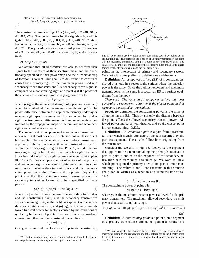
Consider the scenario in Fig. 13. Let np be the exponent that applies to the attenuation along the primary’s attenuation path to point q and ns be the exponent of the secondary at-tenuation path from point s to point q. We want to know which point q on the primary attenuation path is most con-straining. The values a and B are constants in this scenario and b can be written as a function of c using the law of co-sines

2 2 2 cosb a c ac B= + − . The constraining power at point q is ( ) 10 log( )pc q pa np c= − . where pa is the maximum transmit power allowed for the pri-mary transmitter. The maximum allowed secondary transmit power that is still compliant at q is

( ) ( )2 2( , ) 10 log 10 log 2 cosxps s q pa np c pd ns a c ac B= − + + + −

. (2)5 Definition: A constraining point is a point q on a segment

of a primary transmitter’s attenuation path that results in a

5 We are using the full distance between the reference point and each

transmitter although the propagation model is referenced to the 1 meter point from the transmitters. This works so long as the distances are much larger than 1 meter.

Ba

bc

ps

q

Secondary sector boundaries

Attenuation path segment

Fig. 13. A scenario used to evaluate the constraints caused by points on an attenuation path. The point p is the location of a primary transmitter, the point s is the secondary transmitter, and q is a point on the attenuation path. The values of a, b, and c are the lengths of the respective sides and B is the angle formed by the attenuation path and the line from p to s.

local minimum for ps(s,q)x. Movements away from this point are either infeasible or allow a greater transmit power.

Theorem 2. The point qd most distant from the primary transmitter on an attenuation path segment is a constraining point if it is the closest point to s or if

2

2 2

cos2 cos

np c ac Bns a c ac B

−>

+ −,

where c is the distance to that point. Proof. If the qd is the closest point to s then it is most con-

straining since the only feasible moves are toward the primary transmitter so pc(q) increases and the distance from s to q in-creases. Both increase ps(s,q)x. We now want to consider when the end is not the closest point and determine if moving toward p from q on the attenuation path will be more or less constraining. We can determine the relative change of ps(s,q)x

with respect to q by finding the derivative, ( ),

xdps s q

dc.

( ) ( )

( ) ( )2 2

, 5 cos 10ln 10( 2 cos ) ln 10

xdps s q ns c a B np

dc ca c ac B−

= −+ −

. (3)

If the derivative is negative then the allowed secondary trans-mit power increases as c decreases. Using the inequal-

ity( ),

0xdps s q

dc< , the equation

2

2 2

cos2 cos

np c ac Bns a c ac B

−>

+ −

follows from (3). Q.E.D. Definition: An interior constraining point is a constraining

point on an attenuation path that occurs prior to the distant end of a segment of an attenuation path.

An interior constraining point may exist where ( ),

0xdps s q

dc= . In this case equation (3) can be reduced to a

quadratic in c and by using the quadratic equation we find that a local minimum, i.e. a constraining point, may exist at

222 1 cos 2 1 cos 1

2 1

np np np npa B a B ans ns ns ns

cnpns

⎛ ⎞⎛ ⎞ ⎛ ⎞ ⎛ ⎞⎛ ⎞− − + − + −⎜ ⎟ ⎜ ⎟ ⎜ ⎟⎜ ⎟⎜ ⎟⎝ ⎠ ⎝ ⎠ ⎝ ⎠⎝ ⎠⎝ ⎠=⎛ ⎞−⎜ ⎟⎝ ⎠

.

(4) The point is constraining if the radical remains positive. There is still a point when np = ns and can be estimated by adjusting np = np + ε where ε is a small value. Definition: A sector intersection plane is the plane formed by a primary sector boundary and a secondary sector. Definition: The closest attenuation path on a sector intersec-tion plane is the attenuation path through the point closest to s.

Theorem 3: The interior point of the closest attenuation path on a sector intersection plane is the most constraining interior constraining point.

Proof. Assume an interior constraining point qc exists on the closest attenuation path. We will prove that interior con-straining points on all other attenuation paths are less con-

straining than this point. The interior constraining point qc can be one of two types, the closest point on the path segment or a local minimum on the path segment as determined by (4). If there is a interior constraining point on an alternative path then it is either closer, the same distance, or further from p than the constraining point on the closest attenuation path. If the point is closer, then its constraining power is larger than that at qc and since its distance to s is larger it must be less constraining. If at the same distance then it is on an ES with qc and by Theorem 1 qc is the most constraining. Finally if this point is further away from p then the ES through this point will intersect the closest attenuation path further away from p than qc. The point at the intersection of the closest attenuation path and this ES is more constraining than the al-ternative point by Theorem 1 and qc is more constraining than this point by our initial assumption. Q.E.D.

Theorem 4: The most constraining distant constraining point is either the furthest point on the closest attenuation path, the closest point on the primary transmitter right bound-ary, or the furthest point from p on the sector intersection plane.

Proof. When a secondary sector intersects the boundary of a primary sector it will either contain the full primary sector boundary or project a rectangle and create either a quadrilat-eral plane or a quadrilateral plane that is further cut by the boundaries of the primary sector. We will show that points between the three points, the furthest point on the closest at-tenuation path, the closest point on the transmitter right boundary, and the furthest constraining point from p, are not capable of being more restrictive. Say the furthest point on the closest attenuation path qd is restrictive, i.e. it meets the requirements of Theorem 2. No points closer to p than the ES through qd can be more constraining than points at the same distance on the closest attenuation path. If there is a point more constraining, the constraining point on the closest at-tenuation path will not be at the transmitter boundary and the more constraining point must be at the end of another attenua-tion path further away from p. The boundary of the attenua-tion paths is the boundary of the sector intersection plane. This boundary is linear and so rates of change in the permitted secondary transmit power will either increase or decrease monotonically. The end point on this line will be the most constraining and it will either end at the transmitter right boundary or at the furthest constraining point from p. Q.E.D.

Let us now consider the evaluation of the scenarios. In the scenario of Point C, the secondary signal will be strongest at point C and will have much more rapid attenuation locally because of the distance effect as illustrated in Fig. 12. Thus two points should be checked to determine compliance, point C and then the closest point on the ES of the transmitter right boundary. This point is the intersection of the ES with the attenuation path that passes through point C. In the scenario of point D, the constraining point is the closest point on the transmitter right boundary. In this example that point occurs on the intersection of the attenuation path that passes from A to D and the transmitter right boundary. The scenario of point

B is the more difficult to evaluate. Each of the planes formed by the intersection of the sectors and the transmitter right boundary, if intersected, should be checked. When checking a plane, by Theorem 3 we should evaluate the interior constrain-ing point of the closest attenuation path that has an interior point. By Theorem 4 we should check the furthest point on the closest attenuation path and the furthest point on the inter-section plane boundary that extends from the furthest point on the closest attenuation path.

IV. CONCLUSION In this paper we have introduced a method for specifying

location-based spectrum rights, both of primary and secondary users. We have demonstrated the flexibility of this technique to conform rights to cover spatial regions so that there may be spatial reuse. We have described how these rights also pro-vide the criteria for coexistent secondary use of spectrum and then theorems and methods for verifying compliance with these criteria. This type of definition of the spatial RF spec-trum resource enables a much finer spatial and spectral parti-tioning of spectrum and an attendant mathematical model for assessing the interaction of users. It could be added to the ontology used with XG radios to define spectrum use condi-tions and policy. However, it is intended to be the foundation of a dynamic spectrum management utility that would func-tion both as a spectrum use optimizer and a broker for secon-dary markets. With this method, the spectrum resource can be defined, subdivided, managed, and brokered.

APPENDIX A The World Geodetic System – 1984 (WGS 84) defines an

earth centric ellipsoid to serve as the reference datum for loca-tion. It is a global system and is the datum for GPS. Our goal is to take one WGS-84 coordinate and make it the origin of a propagation or power map, create a new coordinate reference at that point where the horizon is the xy plane and the y axis points north, convert other WGS-84 coordinates to that refer-ence system, and then determine direction from the origin to those points. We start by describing the conversion of ellip-soid coordinates to Cartesian. Next we describe the transfor-mation of the reference system at a point defined by WGS-84 coordinates and then the conversion of other WGS-84 points to coordinates in that same reference system. Finally we pro-vide the equations for map directions.

A. Converting Ellipsoid Coordinates to Cartesian Ellipsoids are formed by rotating an ellipse about one of its

axes, the minor axis in the case of geographical reference da-tums. An ellipsoid formed by rotating an ellipse about its mi-nor axis has four measures, the diameter of the semimajor axis, a, the radius of the semiminor axis, b, the flattening, f, and the eccentricity, e. These measures are related as follows.

a bfa−

= (2-1)

2 2

22 2a be f f

a−

= = −

The minor axis is coincident with the axis of rotation of the earth. For a global datum reference the center of the coordi-nate system is located at the center of the earth with the z axis coincident to the minor axis of the spheroid with positive di-rection toward the north pole. The x axis lies on the equato-rial plane pointing toward the meridian passing through the Greenwich Observatory. The positive direction of the y axis is chosen to get a right handed coordinate system. Figure A.1 illustrates the relationship between ellipsoidal and Cartesian coordinates.

There are just two parameters that are needed for specifying an ellipsoid, a and b, a and f, or a and e. Normally a and f are given. Conversion between ellipsoidal and Cartesian coordi-nates requires an initial calculation of the radius of curvature of the prime vertical ν which is a function of latitude. The geodetic latitude is the angle between the plane at the equator and the geodetic normal to the ellipsoid surface. Note that the prime vertical is perpendicular to the ellipsoid surface and extends to the minor axis and may not intersect at the x, y, z origin. This radius of curvature is determined by

( )2 2 2 21 sin 1 2 sin

a a

e f fν

ϕ ϕ= =

− − −

The radius to the point P is ( )hν + . The WGS 84 Cartesian coordinates follow using the equations ( )cos cosx hν ϕ λ= +

( )cos siny hν ϕ λ= +

Long, λ

Lat, ϕ

Greenwich Meridian P = X,Y,Z orλ, ϕ,h

x

y

z

h

Meridian at P

a

b

ν

Fig. A-1. Comparison of Cartesian and ellipsoidal coordinates.

TABLE A-1. THE WGS-84 ELLIPSOID PARAMETERS Parameter Value Units

a 6378137 meters b 6356752.31245 meters f 1

298.257223563

e 0.0818191908426 e2 0.00669437999014

( )( )21 sinz e hν ϕ= − +

Table A-1 lists the WGS 84 parameters. The conversion from WGS 84 Cartesian coordinates back to ellipsoidal coordinates is much more involved. See [8] for the various approaches.

B. Conversion Matrix for the New Cartesian System Conversion to a propagation map reference system centered

at a point follows directly using the WGS 84 longitude and latitude of that point. Figures A-2 through A-4 show the proc-ess. Fig. A-2 shows the new coordinate system with the WGS 84 reference directions. The first rotation illustrated in Fig. A-3 is about the z axis to bring the y axis to the meridian plane that corresponds to the new system’s origin and causes it to point toward the opposite hemisphere. This rotation is (90 + λ)°. This rotation will bring the x axis to the tangential plane pointing easterly. The second rotation illustrated in Fig. A-4 is about the x axis and brings the z axis coincident to the prime vertical and brings the y axis to the tangential plane pointing in the desired direction. The angle of rotation about

the x axis is (90 - ϕ)°. The coordinate conversion matrix for this new system is the matrix defining these rotations

M

sin cos sin cos coscos sin sin sin cos

0 cos sinR

ϕ ϕ λ ϕ λϕ ϕ λ ϕ λ

λ λ

− −⎡ ⎤⎢ ⎥= −⎢ ⎥⎢ ⎥⎣ ⎦

.

The transformation of other WGS 84 Cartesian coordinates to this new system is

M

Map WGS84 WGS84

O

O

O

x x xy R y yz z z

⎛ ⎞⎡ ⎤ ⎡ ⎤ ⎡ ⎤⎜ ⎟⎢ ⎥ ⎢ ⎥ ⎢ ⎥= −⎜ ⎟⎢ ⎥ ⎢ ⎥ ⎢ ⎥⎜ ⎟⎢ ⎥ ⎢ ⎥ ⎢ ⎥⎣ ⎦ ⎣ ⎦ ⎣ ⎦⎝ ⎠

.

where the coordinates xO, yO, and zO are the WGS 84 coordi-nates of the system origin.

C. Determining Directions Directions from the origin to a point follow directly from

their coordinates in the map system. Map longitudes are measured from the x axis about the z axis just as in geodetic systems, however, the latitudes are measured from the z axis rather than from the equatorial plane of the system. This latter convention is used to simplify the map construction. The lon-gitude can be determined directly from the x, y, and z coordi-nates in the map reference system.

1tan yx

θ −= 6

The latitude is determined using

1

2 2 2cos z

x y zφ −=

+ +. 6

More detailed discussion of coordinate transformations can be found in [8].

REFERENCES [1] J. A. Stine, “Enabling secondary spectrum markets using ad hoc and

mesh networking protocols,” Academy Publisher J. of Commun., Vol. 1, No. 1, pp. 26-37. April 2006.

[2] DARPA XG Working Group, “The XG Vision. Request for Comments,” Version 2.0, Prepared by BBN Technologies, Cambridge MA, USA, January 2004.

[3] Shared Spectrum Company News Release “Shared Spectrum Company successfully demonstrates neXt Generation (XG) wireless communica-tions system,“ September 2006. http://www.sharedspectrum.com/inc/ content/press/XG_Demo_News_Release_060918.pdf

[4] DARPA XG Working Group, “XG Policy Language Framework. Re-quest for Comments,” Version 1.0, Prepared by BBN Technologies, Cambridge MA, USA, April 2004.

[5] T. Rappaport, Wireless Communications, Principles and Practice, Sec-ond Edition, Prentice-Hall, Inc, Upper Saddle River, NJ, 2002.

[6] DARPA XG Working Group, “The XG Architectural Framework. Re-quest for Comments,” Version 1.0, Prepared by BBN Technologies, Cambridge MA, USA, July 2003.

[7] L. Berlemann, S. Mangold, G. Jiertz, and B. Walke, “Policy defined spectrum sharing and medium access for cognitive radios,” Academy Pub. J. of Commun. Vol. 1 No. 1, pp. 1- 12, April 2006.

[8] J. A. Stine, MITRE Technology Report “Coordinate systems with trans-formations for Node State Routing,” TBP.

6 The brackets about |θ| and |ϕ| indicate true not coded angles and are used

to be consistent with our notation in section II.D.

Fig. A-4. Second step in conversion to propagation map coordinates is to rotate the system about the x axis to make the z axis coincident with the prime vertical .

Fig. A-3. First step in conversion to propagation map coordinates is to rotate the system about the z axis to point the y axis toward the ellipsoid axis.

Fig. A-2. Starting coordinate system before conversion to propagation map orientation is a translated system with the point at the origin.