NREGs – Correcting for the ‘Accident’ of Birth? A Study of the Determinants of Risk Aversion in

Andhra Pradesh, India

Sweta Gupta

Stu

den

t Pap

er

www.younglives.org.uk MAY 2013

Paper submitted in partial fulfillment of the requirements for the Degree of Master of Science in Economics for Development at the University of Oxford.

The data used come from Young Lives, a longitudinal study of childhood poverty that is tracking the lives of 12,000 children in Ethiopia, India (Andhra Pradesh), Peru and Vietnam over a 15-year period. www.younglives.org.uk

Young Lives is core-funded from 2001 to 2017 by UK aid from the Department for International Development (DFID) and co-funded by the Netherlands Ministry of Foreign Affairs from 2010 to 2014.

The views expressed here are those of the author. They are not necessarily those of the Young Lives project, the University of Oxford, DFID or other funders.

NREGS – CORRECTING FOR THE ‘ACCIDENT’

OF BIRTH?

A study of childhood determinants of risk aversion in Andhra Pradesh, India

By

Sweta Gupta

30 May 2013

Thesis submitted in partial fulfilment of the requirements for the Degree of Master of Science in Economics for Development at the University of Oxford.

Abstract

Economic literature has established the importance of risk attitudes in economic

decision making. The study examines determinants of risk aversion in children. It also

explores the potential of the government to mitigate the effect of shocks, by looking at

the effectiveness of the world’s largest public works program – National Rural

Employment Guarantee Scheme (NREGS). First, it builds a general model of the

determinants of childhood risk aversion. The study finds that the environment –

economic and psychological, that a child is born into plays an important role in

developing the non-cognitive skill - preference for risk. Additionally, economic shocks

do not have a significant impact on risk aversion in childhood years vis-a vis

psychological trauma. Second, the study investigates whether NREGS has been

effective in smoothing income shocks for rural households as would be reflected by less

risk averse children. NREGS has been effective in providing a stable environment to

children resulting in lower risk aversion. Access to the scheme reduced risk aversion in

the Indian sample by 36- 43%. The study employs OLS and Probit models using Young

Lives Round 3 (2009-10) cross-section data from Andhra Pradesh, India, since the risk

questions were only asked in that round. Identification is difficult using only cross-

section data, so I am only able to establish correlations. Further, the Young Lives

dataset contains a rich set of control variables, and Propensity Matching is used to

correct for self-selection into the NREGS. A series of reliability test have also been

conducted to ensure the robustness of results.

TABLE OF CONTENTS

Page #

I. INTRODUCTION 5

II. RELEVANT RESEARCH 7

III. CONCEPTUAL FRAMEWORK –Theory of 8 Childhood Risk Aversion

IV. THE PROGRAM – National Rural Employment 10 Guarantee Scheme (NREGS)

V. DATA AND EXPERIMENTAL DESIGN 11

VI. SUMMARY STATISTICS A) Summary of risk game results 13 B) Summary of descriptive statistics 13

VII. EMPIRICAL STRATEGY

A) Background 15 B) Risk Aversion Measure – Dependent Variable 16 C) Econometric Model – Childhood Determinants Of 17 Risk Aversion D) Econometric Model – Role of NREGS 18

VIII. RESULTS

A) Childhood Determinants of Risk Aversion 20 B) Role of NREGS 23 C) Robustness Checks 25

IX. CONCLUSION 29 REFERENCES 31

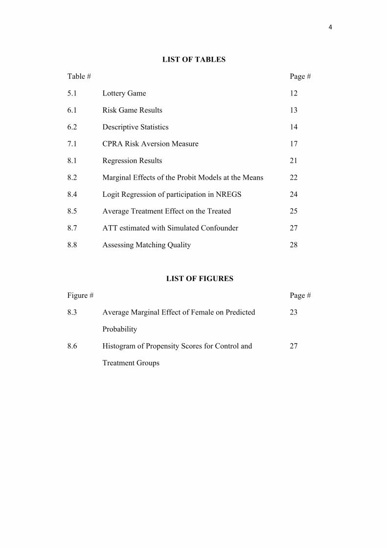
LIST OF TABLES

Table # Page #

5.1 Lottery Game 12

6.1 Risk Game Results 13

6.2 Descriptive Statistics 14

7.1 CPRA Risk Aversion Measure 17

8.1 Regression Results 21

8.2 Marginal Effects of the Probit Models at the Means 22

8.4 Logit Regression of participation in NREGS 24

8.5 Average Treatment Effect on the Treated 25

8.7 ATT estimated with Simulated Confounder 27

8.8 Assessing Matching Quality 28

LIST OF FIGURES

Figure # Page #

8.3 Average Marginal Effect of Female on Predicted 23

Probability

8.6 Histogram of Propensity Scores for Control and 27

Treatment Groups

I. INTRODUCTION

Risk and uncertainty play an important role in economic decision making. If people

were risk neutral or if one could perfectly insure against all risks through well-

developed credit and insurance markets, one would not have to be concerned about such

an analysis. However, empirical literature reveals high risk aversion among individuals.

Harrison, Humphrey and Verschoor (2005) estimate a risk aversion measure of 0.84 for

their Indian sample under the Expected Utility framework, implying a high degree of

risk aversion. As a consequence, in order to understand and predict economic

behaviour, understanding individual risk attitudes is primary. More importantly, one has

to understand the development of risk attitudes through various stages of life. Cognitive

and non-cognitive skills (risk aversion) begin to take shape in early childhood years.

The ‘accident’ of being born into a disadvantaged environment that does not cultivate

cognitive and non-cognitive abilities can place a child at a disadvantage (Heckman,

2000). Since risk attitude is an important determinant of educational attainment and

occupational choice in adulthood, impoverished early environment, resulting in severely

risk averse individuals, becomes a strong predictor of adult failure on various economic

dimensions. A body of research in economics and psychology shows that skill begets

skill (Heckman, 2006). Children who develop extreme risk aversion are likely to remain

so. Hence, it becomes important to study what drives risk behaviour in early years of

growing up and also the need for early intervention to protect the children from

adversities.

In this light, I attempt to study the factors that shape risk attitudes during the critical

period of early childhood. In my sample, 91% of the Indian households identify

themselves as poor holding a Below-Poverty-Line (BPL)1 card. By being placed in an

adverse environment, the young children in my study are more vulnerable to shocks and

adversities than their richer counterparts. This paper not only looks at the determinants

of risk aversion, but also the importance of different factors – psychological and

economic. Interestingly, in the early years, psychological factors such as being included

in games with peers and death of a family member have a significant impact on risk

attitudes.

The second part of the paper analyses the effect of being covered by social protection on

risk aversion in children, while controlling for other household and individual

characteristics. One of the main arguments for social protection is to help the poor cope

with risk in the absence of well-developed insurance and credit markets. The poor are

vulnerable to income shocks which move them in and out of poverty. The National

Rural Employment Scheme (NREGS) is a public works program in India which corrects

for cyclical unemployment, by providing the rural households with employment and

income opportunities. This ensures that the households registered under the program are

protected from income shocks and are able to smooth income and consumption. I

hypothesise that a household which is able to do so will result in less risk averse

children. These children are able to correct for their ‘accident’ of birth as they are less

likely to be exposed to shocks such as, being taken out of school and drop in the

nutritional value of their diet. Results from this study show that households covered by

the NREGS have less risk averse children. This result is important with two regards.

First, it establishes the need for public intervention to mitigate the impact of a

disadvantaged environment. Second, it establishes the effectiveness and success of

NREGS in helping the rural households to protect themselves from shocks.

The paper is organised as follows. Section II describes the relevant research that has

been undertaken around determinants of risk aversion and impact of NREGS,

highlighting the specific contribution of this paper. Section III builds on a theoretical

model of determinants of childhood risk aversion. Section IV gives a brief overview of

the social protection scheme, NREGS. Section V briefly describes the data used in the

study and the lottery game that was played with the children in the sample. Section VI

presents the summary statistics. Section VII describes the econometric model and the

empirical strategy employed. Section VIII presents the empirical results and reliability

tests, and Section IX concludes the paper, emphasizing on the findings.

II. RELEVANT RESEARCH

Considerable research has attempted to explain the factors affecting individuals’ risk

attitudes. Dohmen et al (2011) find that gender, age, height, and parental background

have an economically significant impact on willingness to take risks. Wealth has been

found to have a significant effect on risk aversion in Mette Wik et al (2004). They also

find that females are more risk averse than males in general. Guiso and Paiella (2008)

report that individuals who are exposed to background risks, that is, those who are more

likely to become liquidity constrained or face income uncertainty exhibit a higher

degree of risk aversion. However, these studies focus on risk attitudes in adults. To my

knowledge, there is no relevant research conducted with younger age groups in the area

of risk attitudes. Also, there is scant literature on capturing the effect of social security

schemes or policies in general on risk behaviour. One example is, Hryshko et al (2011)

which shows that policy induced increases in high school graduation rates lead to

significantly fewer individuals being highly risk averse in the next generation.

Dercon (2006) argues that uninsured risk increases poverty through ex ante behavioural

responses affecting activities, assets and technology choices; as well as ex post through

loss of productive assets. He concludes on the basis of this discussion that there is a case

for risk-focussed social protection. Social protection schemes, of which NREGS is one,

provide ex post measures to the poor when they are faced with an adverse shock and

remain uninsured. Given their low income and low assets, the poor are more vulnerable

to risks. At lower levels of income, people are more risk averse, as their welfare is

reduced to larger extent than that of the rich. Studies in India have found that negative

income shocks caused households to withdraw their children from school. This causes

lower educational standards and reduces the income-earning potential of the children

(Jacoby and Skoufias, 1992). Also, in my sample, only 3.8% would try to obtain credit

from the formal sector in the case of hard times (“What would you do in the case of

hard times?”), which can be taken to mean either a non-existent formal credit sector or

little faith in the financial system. Hence, there is strong argument in favour of social

protection – to help the poor cope with shocks reducing their risk aversion and to ensure

proper investment in the child at the critical stage.

With regards to the welfare impact of NREGS in India on rural households, specifically

children, it has been found that NREGS has had a positive effect on child health

outcomes (Uppal, 2009; Dasgupta, 2012). Ravi and Engler (2009) have additionally

looked at the impact of NREGS on food security and savings. Uppal (2009) reports that

NREGS significantly reduced the likelihood of children in the household being required

to work. The stability and increase in nutritional intake introduced by NREGS can

translate into lower risk averse children as they grow up in a safer environment.

This paper makes two contributions to the literature. First, it investigates Heckman’s

theory of life cycle of skill development. Non-cognitive abilities such as, preference for

risk are shaped at an early stage by a host of environmental factors, of which the family

environment is crucial. I test this hypothesis in my sample of 1950 young children in the

age group 8-9 years. To my knowledge, this is the only paper which tries to ascertain

the determinants of childhood risk aversion. Second, most studies have looked at the

effect of NREGS in terms of health outcomes in children. However, I look at the basic

premise for the provision of social protection to comment on its effectiveness. If the

NREGS successfully equipped the rural households to mitigate adverse shocks, the

children would not have to suffer from the ills of child labour, withdrawal from school

or inadequate diet. Thus, the effectiveness of the NREGS would be reflected in less risk

averse children. The results in this paper pose interesting questions for future research -

how does risk aversion behaviour change over the years and which determinants come

to play a dominant role? The results also uphold and strengthen the claims of some

economists – policy interventions that enrich the early years of disadvantaged children

improve non-cognitive skills.

III. CONCEPTUAL FRAMEWORK – THEORY OF CHILDHOOD RISK

AVERSION

Most economic literature has revolved around studying risk behaviour in adults,

neglecting the sensitive childhood phase. Knudsen (2004) shows that early experience

and environment create a structure of neural circuits, which cannot be altered beyond

the sensitive period. Heckman (2000) builds a model of complementarity in investment

in human capital, that is, early investment facilitates the productivity of later

investment. Thus, it is important to study the critical childhood period to enhance our

understanding of how certain attitudes are formed and how they can be adapted using

policy interventions to be conducive to efficient life outcome.

I attempt to build a comprehensive model to study the determinants of one such attitude

- risk aversion. Some of the determinants of risk attitudes described in empirical

literature are gender, age, wealth, parental background and shocks. A study by

Turkheimer et al (2003) found that in poor households, 60% of the variance in cognitive

ability is accounted for by the shared environment. Following from this, I hypothesise

that the environment, both economic and emotional, plays a similar role in the nurturing

of non-cognitive skills, such as, preference for risk among children born in an

economically disadvantaged environment. As suggested by Heckman et al (2006), it is

important to study the role of family income and investment in children in determining

risk attitudes. Hence, I divide the determinants of childhood risk aversion into two

broad categories – economic ( ) and psychological ( . Formally, risk aversion ( ) is

a function of these two and other individual level controls ( ).

One can think of economic factors in terms of income of the household the child is born

into, the area of residence (rural/urban), wealth of the family, access to amenities, and

main occupation pursued by the household head. Also, important to consider are

economic shocks (natural disaster, drought) – shocks which produce volatility in the

income flow. The psychological factors, on the other hand, provide for those factors

that affect the mental functions and behaviour of the child. These factors can range from

having a single parent, interaction with family members, and social inclusion to shocks

such as death of a family member. The individual level characteristics control for

inherent differences in preference for risk – gender and cognitive skills.

It is important to note at this stage, that there are innumerable things that affect risk

attitudes and it is virtually impossible to account for all of them or perfectly predict risk

behaviour. For instance, Heckman et al (2006) argue that skill formation begins in the

womb and may be in part attributable to genes. Since there is no reliable method for

measuring the effect of such factors, despite including a near exhaustive set of

explanatory variables there will be unobservables in the error term driving the risk

behaviour and leading to a bias in the estimated coefficients. Hence, in such a model

studying risk behaviour, one can at most argue for correlation. Additionally, there may

be some degree of correlation between the explanatory variables themselves. For

instance, one cannot expect the wealth of the family to be entirely independent of social

inclusion. A child from a wealthier background may be more accepted in his peer group.

Taking these into account, I present my results as a correlation and study the likelihood

of certain factors in producing more/less risk averse children.

IV. THE PROGRAM – NATIONAL RURAL EMPLOYMENT GUARANTEE

SCHEME (NREGS)2

The NREGS program is the largest public works program in the world which came into

force in February 2006. Public works programs have had numerous objectives including

short term income generation, asset creation, protection from negative shocks and

poverty alleviation (Ninno et al, 2009). The primary objective of the NREGS is to

provide livelihood security to households in the rural area by providing not less than

100 days of guaranteed wage employment in every financial year to every household,

whose adult members volunteer to do unskilled and manual work (GOI, 2009). The

rural household would first have to be registered under the scheme. Thereafter, if the

household wished to undertake work under the scheme, it would have to apply to the

Gram Panchayat, which the Gram Panchayat and the State were legally bound to

provide within 15 days of demand for work. Failure to do so would result in payment of

unemployment allowance by the State. Thus, the scheme introduced an in-built

incentive mechanism for performance on the supply side. It also incorporated time

bound action to meet the demand for work.

The scheme was implemented in a phased manner, initially rolled out in 200 of the

poorest districts in early 2006, making use of a backwardness index - comprising

agricultural productivity per worker, agricultural wage rate, and Scheduled

Caste/Scheduled Tribe population, developed by the Planning Commission. It was

expanded to an additional 130 districts in 2007, and finally expanded to cover the

remaining 274 districts in 2008. For Andhra Pradesh, the program was rolled out first of

all to 13 districts in 2005, then to a further six districts in 2007 and three more districts

in 2008, to cover all 22 districts in the state. Four of my sample districts were covered

by the NREGS in the first phase of implementation in 2005-06 (Anantapur,

Mahaboobnagar, Cuddapah, Karimnagar), with the addition of one more sample district

(Srikakulam) in 2007, and lastly the district of West Godavari was included in 2008.

During 2010–11 Andhra Pradesh provided 274.8 million person days of employment

(Galab et al. 2011).

V. DATA AND EXPERIMENTAL DESIGN

The Young Lives Study follows approximately 3000 children – 1950 children born in

2001-02 and 994 children born in 1994-95 in the state of Andhra Pradesh in India. The

Young Lives Survey has been conducted in three waves – 2001-02, 2006-07 and 2009-

10. A lottery game to elicit risk behaviour was played only the third round, 2009-10,

with the younger cohort (those born in 2001-02). Since I have information on risk

aversion for only the last round, I am unable to exploit the benefits of a panel data and

am restricted to Young Lives Round 3 cross-section data for the first part of my study,

which is to build a model of childhood determinant of risk aversion. In Round 3

extensive child, household and community questionnaires were administered which

enables me to include a host of controls in my regression analysis. For the second part

of my analysis, which is to study the role of NREGS in mitigating the effect of adverse

environment on risk attitudes, I exploit the panel data for conducting a propensity score

matching on my rural sub-sample. Regarding the NREGS, households were asked

whether anybody in the household had registered for the NREGS, whether anybody in

the household has worked under the scheme in the last 12 months, whether employment

was provided within 15 days of registration, whether wages were paid within 15 days of

being employed, whether they benefited from unemployment allowance, and whether

they benefited from childcare facilities at the worksite. The data was collected in

Hyderabad and six districts of Andhra Pradesh, chosen to represent the different

geographical regions, levels of development and population characteristics (Young

Lives website), while households were chosen randomly amongst those which had

children born in the stipulated years.

In Young Lives Round 3 data, risk aversion information was collected for the younger

cohort in India. The children were presented with 6 options. The lottery was not played

with real money as that would have been ethicallyincorrect, but the children were asked

to pretend that they were dealing with real money. A coin was flipped and depending on

the lottery choice of the child and whether the coin landed heads or tails, the child won

an amount. With the first choice, if the coin landed on heads, the child won 50 rupees,

and if it landed on tails, the child also got 50 rupees. With the second choice, if the coin

landed on heads, 100 rupees was won, and if it landed on tails, only 40 rupees was won.

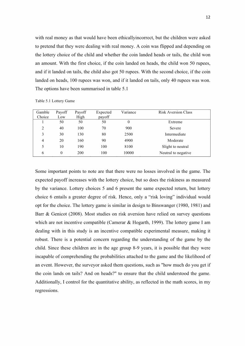
The options have been summarised in table 5.1

Table 5.1 Lottery Game

Gamble Choice

Payoff Low

Payoff High

Expected payoff

Variance Risk Aversion Class

1 50 50 50 0 Extreme 2 40 100 70 900 Severe 3 30 130 80 2500 Intermediate 4 20 160 90 4900 Moderate 5 10 190 100 8100 Slight to neutral 6 0 200 100 10000 Neutral to negative

Some important points to note are that there were no losses involved in the game. The

expected payoff increases with the lottery choice, but so does the riskiness as measured

by the variance. Lottery choices 5 and 6 present the same expected return, but lottery

choice 6 entails a greater degree of risk. Hence, only a “risk loving” individual would

opt for the choice. The lottery game is similar in design to Binswanger (1980, 1981) and

Barr & Genicot (2008). Most studies on risk aversion have relied on survey questions

which are not incentive compatible (Camerar & Hogarth, 1999). The lottery game I am

dealing with in this study is an incentive compatible experimental measure, making it

robust. There is a potential concern regarding the understanding of the game by the

child. Since these children are in the age group 8-9 years, it is possible that they were

incapable of comprehending the probabilities attached to the game and the likelihood of

an event. However, the surveyor asked them questions, such as "how much do you get if

the coin lands on tails? And on heads?" to ensure that the child understood the game.

Additionally, I control for the quantitative ability, as reflected in the math scores, in my

regressions.

VI. SUMMARY STATISTICS

A) Summary of Risk Game Results

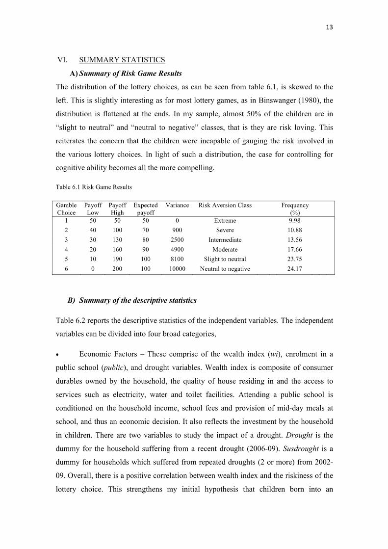
The distribution of the lottery choices, as can be seen from table 6.1, is skewed to the

left. This is slightly interesting as for most lottery games, as in Binswanger (1980), the

distribution is flattened at the ends. In my sample, almost 50% of the children are in

“slight to neutral” and “neutral to negative” classes, that is they are risk loving. This

reiterates the concern that the children were incapable of gauging the risk involved in

the various lottery choices. In light of such a distribution, the case for controlling for

cognitive ability becomes all the more compelling.

Table 6.1 Risk Game Results

Gamble Choice

Payoff Low

Payoff High

Expected payoff

Variance Risk Aversion Class Frequency (%)

1 50 50 50 0 Extreme 9.98 2 40 100 70 900 Severe 10.88 3 30 130 80 2500 Intermediate 13.56 4 20 160 90 4900 Moderate 17.66 5 10 190 100 8100 Slight to neutral 23.75 6 0 200 100 10000 Neutral to negative 24.17

B) Summary of the descriptive statistics

Table 6.2 reports the descriptive statistics of the independent variables. The independent

variables can be divided into four broad categories,

• Economic Factors – These comprise of the wealth index (wi), enrolment in a

public school (public), and drought variables. Wealth index is composite of consumer

durables owned by the household, the quality of house residing in and the access to

services such as electricity, water and toilet facilities. Attending a public school is

conditioned on the household income, school fees and provision of mid-day meals at

school, and thus an economic decision. It also reflects the investment by the household

in children. There are two variables to study the impact of a drought. Drought is the

dummy for the household suffering from a recent drought (2006-09). Susdrought is a

dummy for households which suffered from repeated droughts (2 or more) from 2002-

09. Overall, there is a positive correlation between wealth index and the riskiness of the

lottery choice. This strengthens my initial hypothesis that children born into an

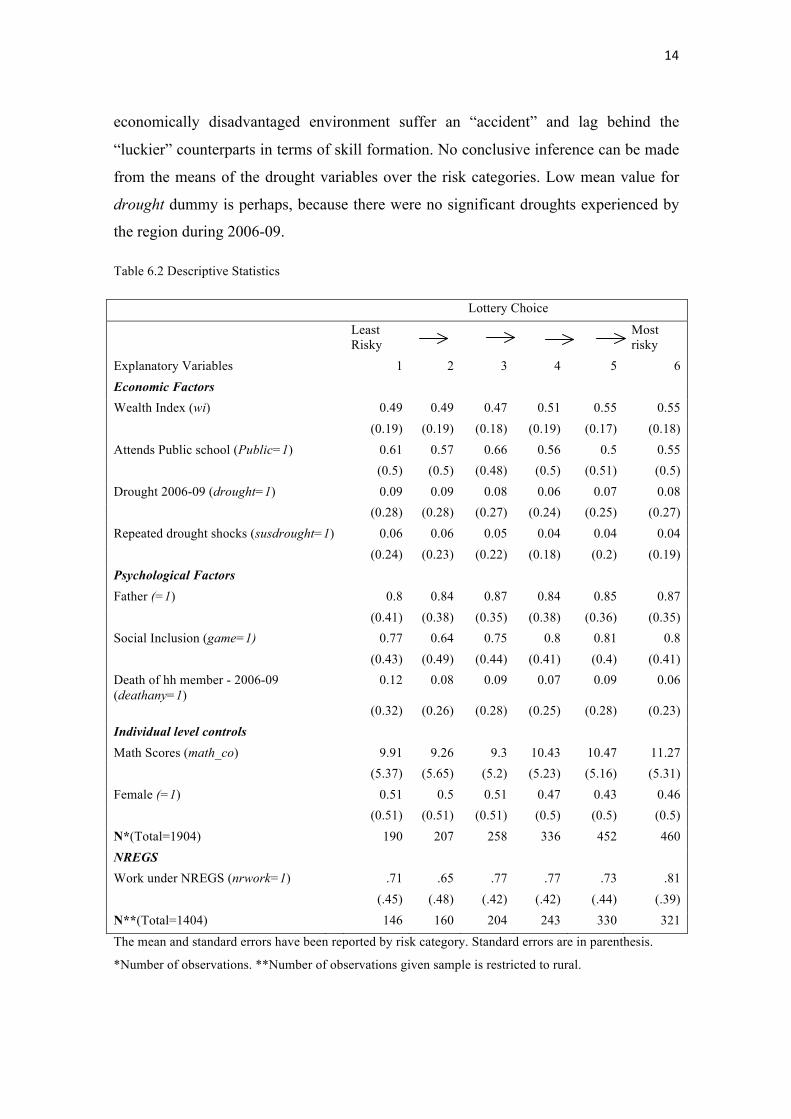
economically disadvantaged environment suffer an “accident” and lag behind the

“luckier” counterparts in terms of skill formation. No conclusive inference can be made

from the means of the drought variables over the risk categories. Low mean value for

drought dummy is perhaps, because there were no significant droughts experienced by

the region during 2006-09.

Table 6.2 Descriptive Statistics

Lottery Choice

Least Risky

Most risky

Explanatory Variables 1 2 3 4 5 6 Economic Factors Wealth Index (wi) 0.49 0.49 0.47 0.51 0.55 0.55 (0.19) (0.19) (0.18) (0.19) (0.17) (0.18) Attends Public school (Public=1) 0.61 0.57 0.66 0.56 0.5 0.55 (0.5) (0.5) (0.48) (0.5) (0.51) (0.5) Drought 2006-09 (drought=1) 0.09 0.09 0.08 0.06 0.07 0.08 (0.28) (0.28) (0.27) (0.24) (0.25) (0.27) Repeated drought shocks (susdrought=1) 0.06 0.06 0.05 0.04 0.04 0.04 (0.24) (0.23) (0.22) (0.18) (0.2) (0.19) Psychological Factors Father (=1) 0.8 0.84 0.87 0.84 0.85 0.87 (0.41) (0.38) (0.35) (0.38) (0.36) (0.35) Social Inclusion (game=1) 0.77 0.64 0.75 0.8 0.81 0.8 (0.43) (0.49) (0.44) (0.41) (0.4) (0.41) Death of hh member - 2006-09 (deathany=1)

0.12 0.08 0.09 0.07 0.09 0.06

(0.32) (0.26) (0.28) (0.25) (0.28) (0.23) Individual level controls Math Scores (math_co) 9.91 9.26 9.3 10.43 10.47 11.27 (5.37) (5.65) (5.2) (5.23) (5.16) (5.31) Female (=1) 0.51 0.5 0.51 0.47 0.43 0.46 (0.51) (0.51) (0.51) (0.5) (0.5) (0.5) N*(Total=1904) 190 207 258 336 452 460 NREGS Work under NREGS (nrwork=1) .71 .65 .77 .77 .73 .81 (.45) (.48) (.42) (.42) (.44) (.39) N**(Total=1404) 146 160 204 243 330 321 The mean and standard errors have been reported by risk category. Standard errors are in parenthesis.

*Number of observations. **Number of observations given sample is restricted to rural.

• Psychological Factors – These include dummies for being included in the game

with peers (game), meeting father daily (father) and if the household suffered a loss of

the family member in recent past (deathany). On the whole, the mean for the variables,

father and game, increases with the riskiness of the lottery choice, pointing at the

importance of emotional experiences in shaping risk attitudes.

• Individual controls – Math scores (math_co) controls for the mathematic ability

of the child in comprehending the likelihood of winning an amount in the different

lottery choices. Female dummy controls for the gender. Empirical literature seems to

suggest that females on an average are more risk averse than males. A similar trend is

noticeable from the summary statistics – a lower number of females opt for the riskiest

lottery choice. Since the children in my sample are very young, it interesting to see that

the distinction between male and female has already set in. Dohmen et al (2007) find

that risk aversion is correlated with cognitive ability. In my study too, as is clear from

the descriptive statistic, children with higher mean math scores opt for riskier options.

• Role of NREGS – To study the impact of social protection program, NREGS, I

use the variable nrwork which takes the value of 1 if the household found work under

the NREGS. The mean value for each risk category is high, implying a high degree of

participation in the program. Also, noticeable is a higher mean value for the riskiest

category vis-à-vis the least risky category.

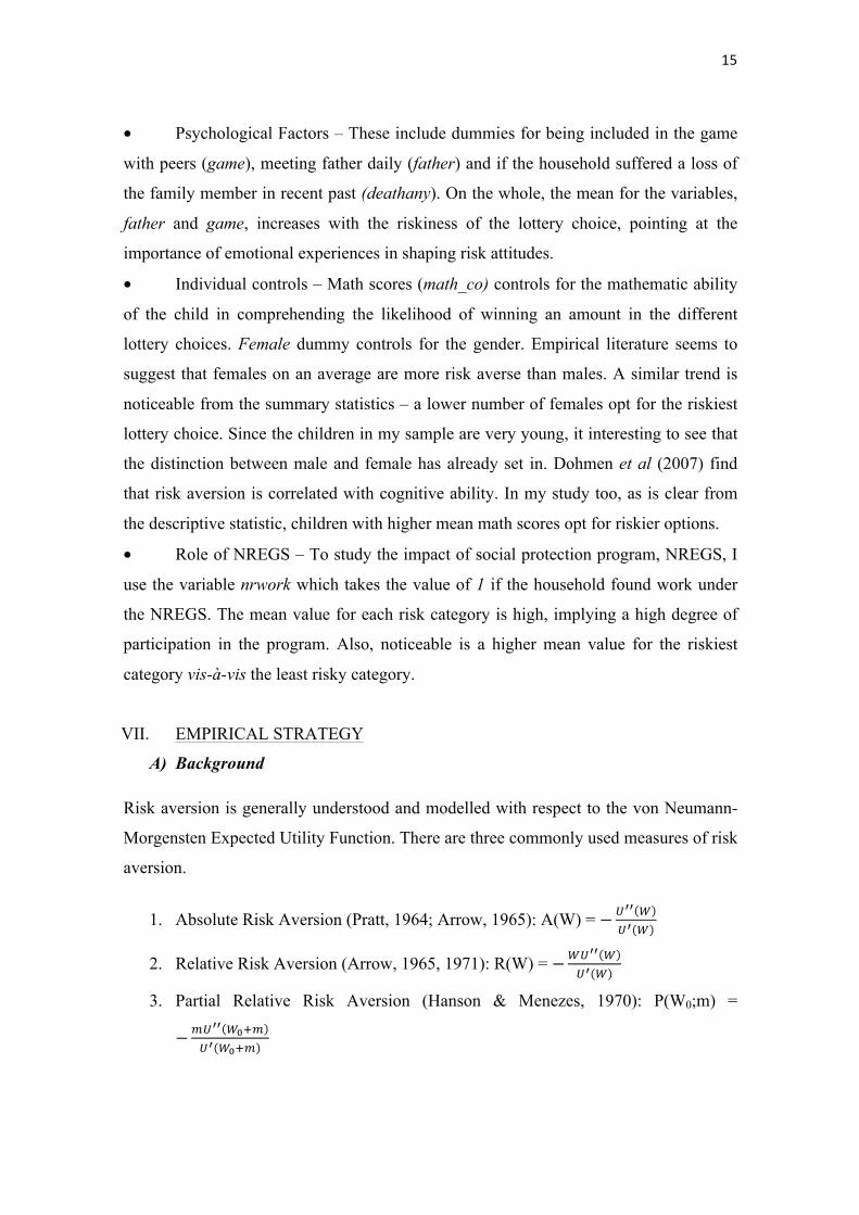
VII. EMPIRICAL STRATEGY

A) Background

Risk aversion is generally understood and modelled with respect to the von Neumann-

Morgensten Expected Utility Function. There are three commonly used measures of risk

aversion.

1. Absolute Risk Aversion (Pratt, 1964; Arrow, 1965): A(W) =

2. Relative Risk Aversion (Arrow, 1965, 1971): R(W) =

3. Partial Relative Risk Aversion (Hanson & Menezes, 1970): P(W0;m) =

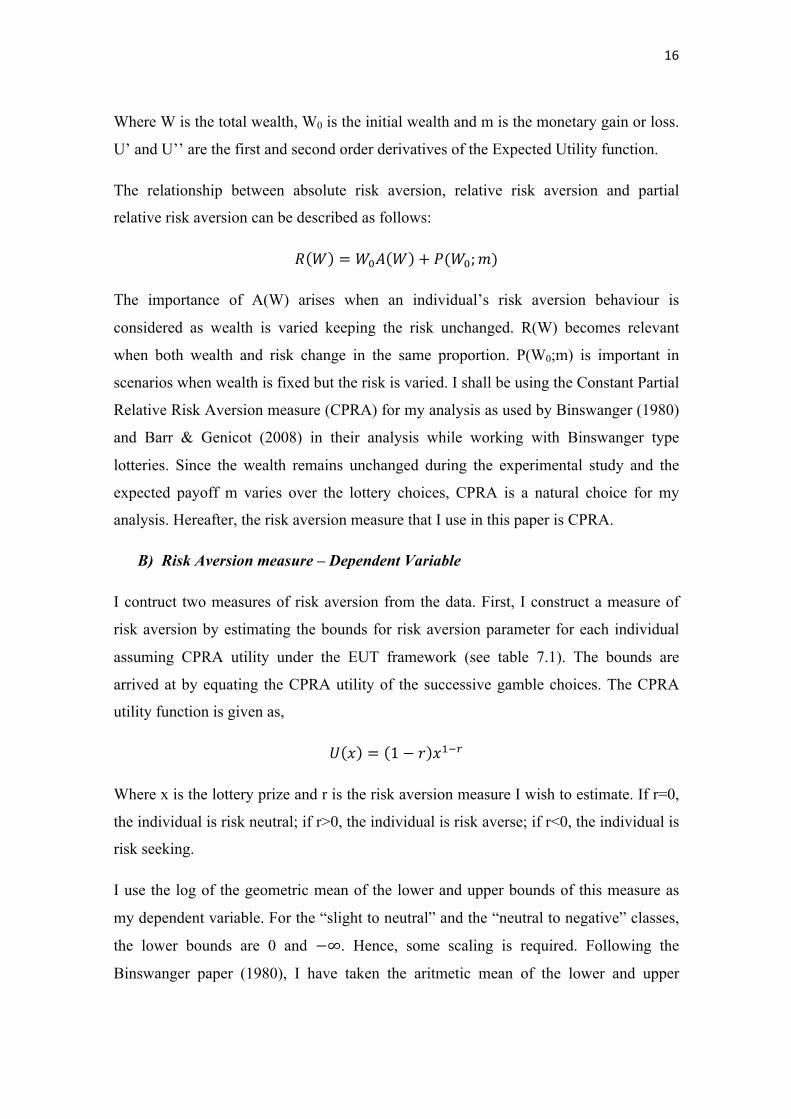
Where W is the total wealth, W0 is the initial wealth and m is the monetary gain or loss.

U’ and U’’ are the first and second order derivatives of the Expected Utility function.

The relationship between absolute risk aversion, relative risk aversion and partial

relative risk aversion can be described as follows:

The importance of A(W) arises when an individual’s risk aversion behaviour is

considered as wealth is varied keeping the risk unchanged. R(W) becomes relevant

when both wealth and risk change in the same proportion. P(W0;m) is important in

scenarios when wealth is fixed but the risk is varied. I shall be using the Constant Partial

Relative Risk Aversion measure (CPRA) for my analysis as used by Binswanger (1980)

and Barr & Genicot (2008) in their analysis while working with Binswanger type

lotteries. Since the wealth remains unchanged during the experimental study and the

expected payoff m varies over the lottery choices, CPRA is a natural choice for my

analysis. Hereafter, the risk aversion measure that I use in this paper is CPRA.

B) Risk Aversion measure – Dependent Variable

I contruct two measures of risk aversion from the data. First, I construct a measure of

risk aversion by estimating the bounds for risk aversion parameter for each individual

assuming CPRA utility under the EUT framework (see table 7.1). The bounds are

arrived at by equating the CPRA utility of the successive gamble choices. The CPRA

utility function is given as,

Where x is the lottery prize and r is the risk aversion measure I wish to estimate. If r=0,

the individual is risk neutral; if r>0, the individual is risk averse; if r<0, the individual is

risk seeking.

I use the log of the geometric mean of the lower and upper bounds of this measure as

my dependent variable. For the “slight to neutral” and the “neutral to negative” classes,

the lower bounds are 0 and . Hence, some scaling is required. Following the

Binswanger paper (1980), I have taken the aritmetic mean of the lower and upper

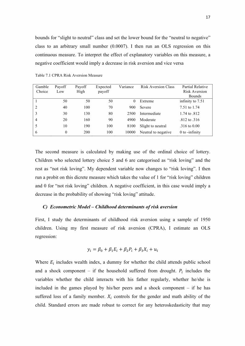
bounds for “slight to neutral” class and set the lower bound for the “neutral to negative”

class to an arbitrary small number (0.0007). I then run an OLS regression on this

continuous measure. To interpret the effect of explanatory variables on this measure, a

negative coefficient would imply a decrease in risk aversion and vice versa

Table 7.1 CPRA Risk Aversion Measure

Gamble Choice

Payoff Low

Payoff High

Expected payoff

Variance Risk Aversion Class Partial Relative Risk Aversion

Bounds 1 50 50 50 0 Extreme infinity to 7.51 2 40 100 70 900 Severe 7.51 to 1.74 3 30 130 80 2500 Intermediate 1.74 to .812 4 20 160 90 4900 Moderate .812 to .316 5 10 190 100 8100 Slight to neutral .316 to 0.00 6 0 200 100 10000 Neutral to negative 0 to -infinity

The second measure is calculated by making use of the ordinal choice of lottery.

Children who selected lottery choice 5 and 6 are categorised as “risk loving” and the

rest as “not risk loving”. My dependent variable now changes to “risk loving”. I then

run a probit on this dicrete measure which takes the value of 1 for “risk loving” children

and 0 for “not risk loving” children. A negative coefficient, in this case would imply a

decrease in the probability of showing “risk loving” attitude.

C) Econometric Model – Childhood determinants of risk aversion

First, I study the determinants of childhood risk aversion using a sample of 1950

children. Using my first measure of risk aversion (CPRA), I estimate an OLS

regression:

Where includes wealth index, a dummy for whether the child attends public school

and a shock component – if the household suffered from drought. includes the

variables whether the child interacts with his father regularly, whether he/she is

included in the games played by his/her peers and a shock component – if he has

suffered loss of a family member. controls for the gender and math ability of the

child. Standard errors are made robust to correct for any heteroskedasticity that may

arise due to correlation between unobservables and the dependent variable. They are

also clustered at the sub-district level (21 mandals) to correct for district fixed effects –

children belonging to a certain mandal may be affected by the same heterogeneity of

unobservables (law and order, political stability) resulting is similar variance within

mandals.

Using the second measure, I set up a probit model. The dependent variable is “risk

loving”. Although I could have used a logit model, empirically it makes little difference

(Cameron &Trivedi, 2006). Building on the probit model, the dependent variable, ,

takes the value of 1 if the child is “risk loving” and 0 if he is not. Thus,

is a standard normal cumulative distribution function. This is a non-linear model

which I estimate using log-likelihood function. The estimators one gets from Maximum

Likelihood function are consistent, asymptotically efficient and asymptotically normal.

However, this is conditioned on the fact that the model has been correctly satisfied.

Non-normality or heteroskedasticity of the error term might lead to inconsistent

estimators. I report the Wald test in the results section to examine for possible

misspecification of the model.

D) Econometric Model – Role of NREGS

The second part of my analysis is to study the effectiveness of NREGS in helping

households to cope with shocks and smooth income, resulting in less risk averse

children. Since the scheme was available to only rural households, I restrict my sample

to rural areas. 73.8% of the sample households reside in rural regions and are thus,

eligible for the scheme. Restricting my study to the rural areas, would mean that I am

incapable of making a policy advice of extending the NREGS program to the public in

general due to its success in rural households in smoothing income. However, that is not

the point of this analysis. My analysis is restricted to study the effectiveness of the

program among the people who had access to it.

The most important concern in dealing with the effectiveness of NREGS is one of self-

selection, and it is the most challenging to deal with. Self-selection bias occurs in my

analysis because participation in the NREGS is not random. This bias is due to two

factors. First, the NREGS was implemented in a targeted fashion, targeting the most

backward districts first. To correct for this, I cluster the standard errors at the district

level. Household living in a certain district which received the NREGS prior to other

districts, might behave in a similar fashion different from households in other districts.

Second, household were free to register for the program. This introduces self-selection

into the program. I deal with this issue by looking at whether the household secured

work under the scheme rather than whether it has a job card under the scheme. Once the

household registers for the program, it has created a demand for employment. However,

getting a job under the scheme is a supply side phenomenon which is arguably

exogenous to my model. Additionally, I estimate the average treatment effect of

participation in the NREGS by estimating propensity score. The method implemented

for Propensity Score Matching (PSM) is described below.

The matching approach is one possible solution to the selection problem. The basic idea

is to match the non-participants with the participants who are similar terms of

observable characteristics . However, since conditioning on all relevant covariates

would result in a high dimension of , Rosenbaum and Rubin (1983) suggested the use

of balancing scores. One such balancing score is the propensity score which measures

the probability of participating in a program given the observable characteristics, .

Where P(X) is the propensity score and D is the dummy for having received the

treatment, that is, of being covered by the NREGS. For the binary treatment case, where

probability of participation versus non-participation is to estimated, logit and probit

models usually yield similar results (Caliendo & Kopeinig, 2005). Hence, the choice is

not too critical, even though the logit distribution has more density mass in the bounds. I

use the logit model to estimate the propensity score. In my estimation, I use the

observable characteristics which would affect both participation in NREGS and the risk

aversion in children from Young Lives Round 2 data (2006-07).

Once the propensity score has been obtained, I carry out matching using two methods –

5-Nearest Neighbour and Kernel Density. I use the optimal bandwidth value (0.044) as

suggested by Silverman (1984) to carry out Epanechnikov kernel density matching. The

impact of the program or the average treatment effect on the treated is given as,

Where is the measure of risk aversion in children belonging to participating (treated)

households, is the measure of risk aversion in children belonging to non-

participating (control) households, and denote the treated and control groups

respectively, and denotes the weights assigned to the control group matches -

kernel-weights which give higher weights to the closer matches of non-participants and

5-nearest neighbour provide uniform weights. Using only 1 nearest neighbour may

produce bad matches as high score participants may be matched with low score

participants. This concern is subsumed by allowing for matching with replacement and

multiple neighbours. Furthermore, kernel density matching is used which uses more

information and relies on non-parametric matching.

VIII. RESULTS

A) Childhood Determinants of Risk Aversion

Table 8.1 reports the results of regressions for both OLS and probit models.

Additionally, the Wald test has also been reported for the probit model. The null

hypothesis under the Wald test is that the variables of interest are all insignificant. The

small p-value reported in my results rejects the null. Also, one can note that the

predicted value for being “risk loving” under both probit specifications is very close to

the actual value.

Columns 1 (OLS) and 2 (probit) of table 8.1 report results of regressions with shocks

from the recent past - death of a household member and drought. Although death of a

household member makes the child more risk averse (significant coefficient at 5% level

of significance under OLS), the effect is not strong enough to push him out of “risk

loving” category (insignificance under probit). This is to say that the child who has

suffered a loss would still be willing to take risks but not to the same extent as those

who haven’t been subjected to same personal grief. The insignificant effect of an

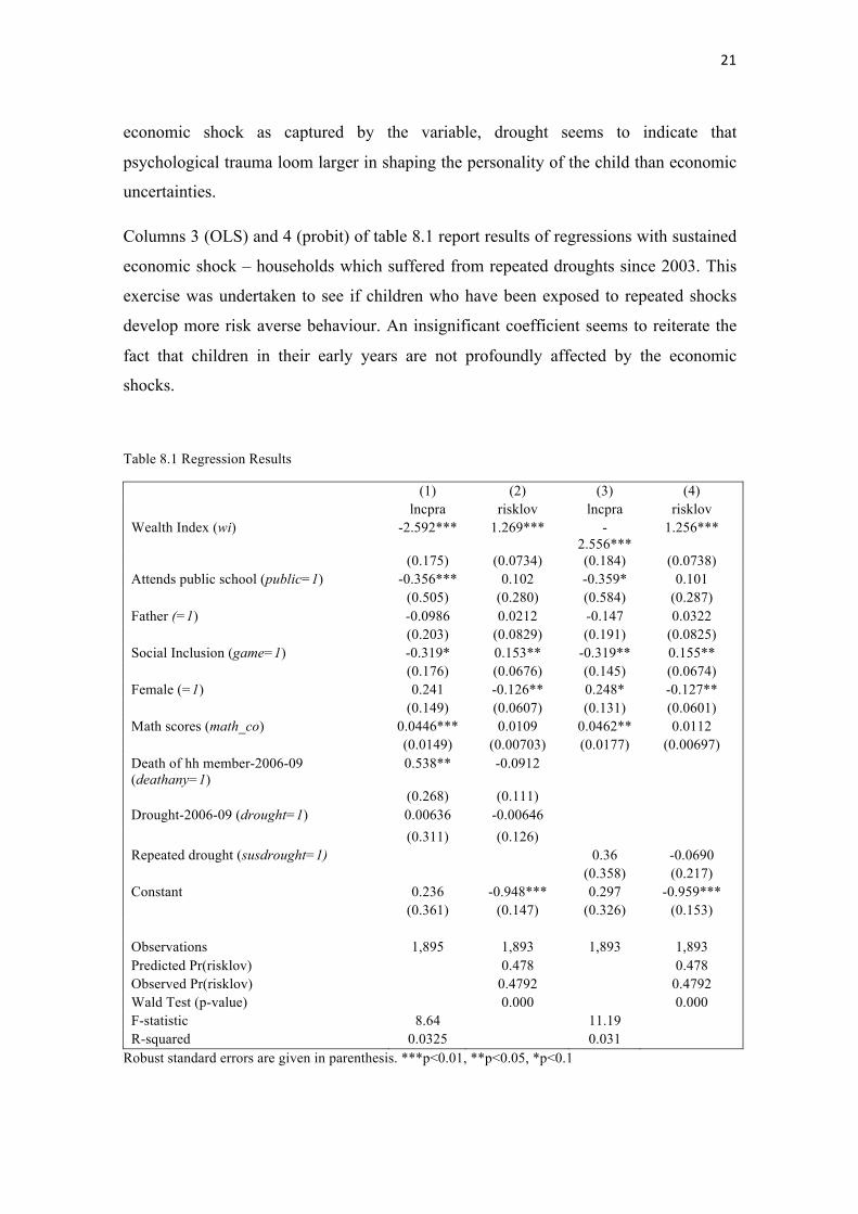
economic shock as captured by the variable, drought seems to indicate that

psychological trauma loom larger in shaping the personality of the child than economic

uncertainties.

Columns 3 (OLS) and 4 (probit) of table 8.1 report results of regressions with sustained

economic shock – households which suffered from repeated droughts since 2003. This

exercise was undertaken to see if children who have been exposed to repeated shocks

develop more risk averse behaviour. An insignificant coefficient seems to reiterate the

fact that children in their early years are not profoundly affected by the economic

shocks.

Table 8.1 Regression Results

(1) (2) (3) (4) lncpra risklov lncpra risklov

Wealth Index (wi) -2.592*** 1.269*** -2.556***

1.256***

(0.175) (0.0734) (0.184) (0.0738) Attends public school (public=1) -0.356*** 0.102 -0.359* 0.101 (0.505) (0.280) (0.584) (0.287) Father (=1) -0.0986 0.0212 -0.147 0.0322 (0.203) (0.0829) (0.191) (0.0825) Social Inclusion (game=1) -0.319* 0.153** -0.319** 0.155** (0.176) (0.0676) (0.145) (0.0674) Female (=1) 0.241 -0.126** 0.248* -0.127** (0.149) (0.0607) (0.131) (0.0601) Math scores (math_co) 0.0446*** 0.0109 0.0462** 0.0112 (0.0149) (0.00703) (0.0177) (0.00697) Death of hh member-2006-09 (deathany=1)

0.538** -0.0912

(0.268) (0.111) Drought-2006-09 (drought=1) 0.00636 -0.00646 (0.311) (0.126) Repeated drought (susdrought=1) 0.36 -0.0690 (0.358) (0.217) Constant 0.236 -0.948*** 0.297 -0.959*** (0.361) (0.147) (0.326) (0.153) Observations 1,895 1,893 1,893 1,893 Predicted Pr(risklov) 0.478 0.478 Observed Pr(risklov) 0.4792 0.4792 Wald Test (p-value) 0.000 0.000 F-statistic 8.64 11.19 R-squared 0.0325 0.031

Robust standard errors are given in parenthesis. ***p<0.01, **p<0.05, *p<0.1

Children who attended public school are less risk averse than those attending private

school (significant coefficients in columns 1 and 3). This can be explained through the

Mid-Day Meal Scheme (MDMS) operational in India. Public schools provide meals to

the children. Hence, children attending public school, did not suffer from a drop in

nutritional intake due to economic shocks. Singh, Park and Dercon (2012) report

significant gains in health for Indian children covered by the MDMS in the face of a

drought. Following from this, public schools serve as a cushion from adverse shocks

resulting in a more stable and safer environment for children. This safety net might

explain the lower risk aversion that my regression analysis captures.

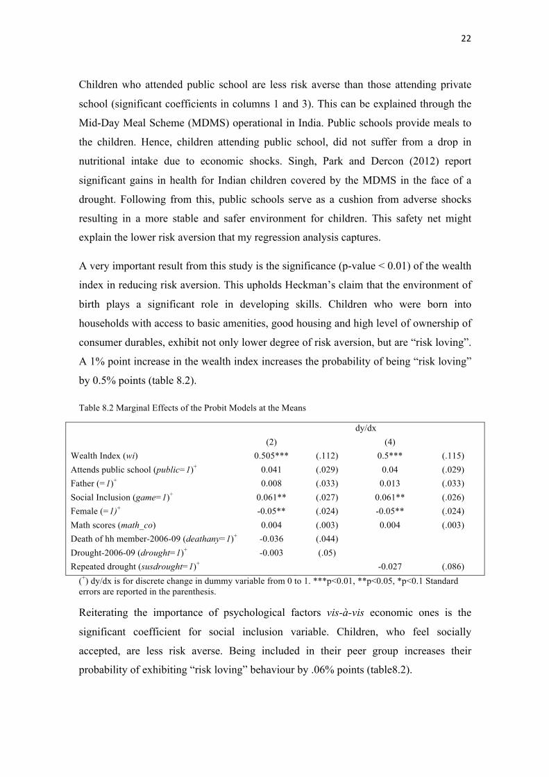
A very important result from this study is the significance (p-value < 0.01) of the wealth

index in reducing risk aversion. This upholds Heckman’s claim that the environment of

birth plays a significant role in developing skills. Children who were born into

households with access to basic amenities, good housing and high level of ownership of

consumer durables, exhibit not only lower degree of risk aversion, but are “risk loving”.

A 1% point increase in the wealth index increases the probability of being “risk loving”

by 0.5% points (table 8.2).

Table 8.2 Marginal Effects of the Probit Models at the Means

dy/dx (2) (4) Wealth Index (wi) 0.505*** (.112) 0.5*** (.115) Attends public school (public=1)+ 0.041 (.029) 0.04 (.029) Father (=1)+ 0.008 (.033) 0.013 (.033) Social Inclusion (game=1)+ 0.061** (.027) 0.061** (.026) Female (=1)+ -0.05** (.024) -0.05** (.024) Math scores (math_co) 0.004 (.003) 0.004 (.003) Death of hh member-2006-09 (deathany=1)+ -0.036 (.044) Drought-2006-09 (drought=1)+ -0.003 (.05) Repeated drought (susdrought=1)+ -0.027 (.086)

(+) dy/dx is for discrete change in dummy variable from 0 to 1. ***p<0.01, **p<0.05, *p<0.1 Standard errors are reported in the parenthesis.

Reiterating the importance of psychological factors vis-à-vis economic ones is the

significant coefficient for social inclusion variable. Children, who feel socially

accepted, are less risk averse. Being included in their peer group increases their

probability of exhibiting “risk loving” behaviour by .06% points (table8.2).

Interesting to note is the difference between males and females in their risk taking

attitude. Females are more risk averse than males. The CPRA risk aversion measure is

24.8% higher for females implying a higher degree of risk aversion. Also, as reported in

table 8.2, the probability of choosing the riskiest bet reduces by 0.05% points in the case

of females. Figure 8.3 plots the marginal effect of the difference between males and

females on the probability of being “risk loving” as the wealth index increases. As we

can see, at all levels of wealth index, females are more risk averse. However, interesting

to note is that at very high and very low levels of wealth index, the marginal effect of

being a female on risk attitude is the same. This seems to suggest that at the extremes,

economic standing plays a more dominant role in predicting risk attitudes. This

strengthens Heckman’s argument for an early childhood investment to correct for the

“accident” of birth into an economically poor household.

Figure 8.3 Average Marginal Effects of Female on Predicted Probability

B) Role of NREGS

Table 8.4 reports the results of the logit regression to estimate the propensity score. The

sample has been restricted only to rural household (1404 observations) in this section,

since only rural households had access to the scheme. The mean propensity score is

0.682 (with a standard deviation of 0.225) which is comparable to the mean score from

the sample (0.683 with a standard deviation of 0.465). Table 8.4 Logit Regression of participation in NREGS

/03

/02:

/028

/026

/024

2

2 03 04 05 06 07 08 09 0: 0; 3y gcnvj "kpf gz

Cxgtci g"Octi kpcn"Ghhgevu"qh"hgo cng"y kvj "; 7’ "EKu

Covariates Estimate Std. Err.

Scheduled Caste 0.945*** (0.241)

Scheduled Tribe 0.755*** (0.260)

Other Backward Class 0.404** (0.204)

Parent's Education (Average Years) -0.056*** (0.021)

Salaried Employee -0.119 (0.173)

Main Source of Income : Agriculture 0.888*** (0.138)

Hindu 2.233 (0.905)

Muslim 1.921 (0.996)

Income from Pension -0.258 (0.397)

Income from Social Security (other than NREGS)

-0.239 (0.175)

Participation in Indira Kranthi Patham (IKP) -0.105 (0.230)

Easily Raise Rs. 1000 -0.344** (0.138)

Suffered Increase in Input Prices 0.152 (0.243)

Suffered Drought 0.229 (0.148)

Suffered Crop Failure 0.296 (0.185)

Suffered Livestock Death 0.094 (0.254)

Housing Services Index -2.796*** (0.473)

Consumer Durables Index -1.141** (0.468)

Intercept -0.220 0.960

***p<0.01 **p<0.5 *p<0.1. Standard errors are reported in parentheses. The dependent variable is the binomial indicator whether a household participated in the NREGS (1 = participation).

The results of the propensity score estimation are in accordance with the economic

literature and research undertaken to study the impact of the NREGS. Uppal (2009)

noted that belonging to Scheduled Caste and Other Backward Class, as well as being

engaged in agriculture increase the probability of participation into the program. Similar

results hold for my analysis. Belonging to a socio-economically deprived section of the

society has a strong positive impact on participation. Also, housing services index and

consumer durables index, a good proxy for the economic standing of the household, are

negatively correlated with program participation. This seems to suggest that the self-

targeting mechanism of the scheme works well with the disadvantaged communities

enrolling into the program. Being engaged in agriculture may leave the people

seasonally unemployed, thereby increasing the chances of such people participating in

the program. This is in unison with the findings of Ravi and Engler (2009). An

interesting variable is the ease with which household can raise Rs.1000 reflecting the

liquidity constraint. Households which can easily raise Rs. 1000 are less liquidity

constrained and are less likely to register for NREGS.

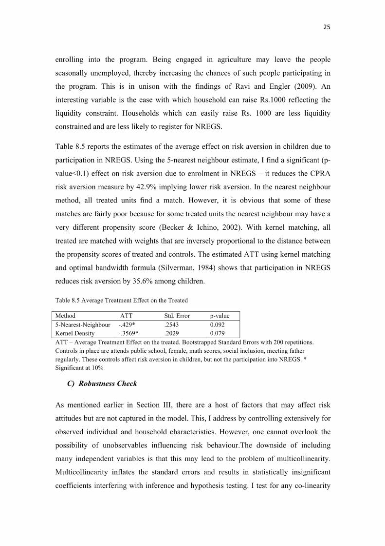
Table 8.5 reports the estimates of the average effect on risk aversion in children due to

participation in NREGS. Using the 5-nearest neighbour estimate, I find a significant (p-

value<0.1) effect on risk aversion due to enrolment in NREGS – it reduces the CPRA

risk aversion measure by 42.9% implying lower risk aversion. In the nearest neighbour

method, all treated units find a match. However, it is obvious that some of these

matches are fairly poor because for some treated units the nearest neighbour may have a

very di erent propensity score (Becker & Ichino, 2002). With kernel matching, all

treated are matched with weights that are inversely proportional to the distance between

the propensity scores of treated and controls. The estimated ATT using kernel matching

and optimal bandwidth formula (Silverman, 1984) shows that participation in NREGS

reduces risk aversion by 35.6% among children.

Table 8.5 Average Treatment Effect on the Treated

Method ATT Std. Error p-value 5-Nearest-Neighbour -.429* .2543 0.092 Kernel Density -.3569* .2029 0.079 ATT – Average Treatment Effect on the treated. Bootstrapped Standard Errors with 200 repetitions. Controls in place are attends public school, female, math scores, social inclusion, meeting father regularly. These controls affect risk aversion in children, but not the participation into NREGS. * Significant at 10%

C) Robustness Check

As mentioned earlier in Section III, there are a host of factors that may affect risk

attitudes but are not captured in the model. This, I address by controlling extensively for

observed individual and household characteristics. However, one cannot overlook the

possibility of unobservables influencing risk behaviour.The downside of including

many independent variables is that this may lead to the problem of multicollinearity.

Multicollinearity inflates the standard errors and results in statistically insignificant

coefficients interfering with inference and hypothesis testing. I test for any co-linearity

by looking at the OLS regression and variance of influence (VIF) analysis and find that

the VIF is less than 2 for each variable. A common rule of thumb is that if VIF ,

multicollinearity is high. Hence, for my results, multicollinearity is not a cause of

worry.

Second, 24% of the children in my sample choose the riskiest lottery choice (Gamble

choice 6), although it represents the same expected payoff as the less risky lottery

choice 5. This may not be considered rational behaviour. I conduct a robustness check,

by excluding the respondents (460 observations) who chose the riskiest option and

estimating the OLS and probit models on the reduced sample. The results showed that

there is no difference in the sign or statistical significance of the coefficients. Hence, I

can safely conclude that the results reported in my study are not driven by the

respondents opting for the “inefficient” choice 6.

Third, PSM relies on two assumptions – conditional independence assumption (CIA)

and overlap assumption. According to CIA, the potential outcome is independent of the

treatment assignment given the vector of observable characteristics. This is commonly

known as the “unconfoundedness” or “selection on observables” assumption. In

addition to this, is required the overlap condition which ensures that for each treated

unit, there is a control unit with the same observables. Rosenbaum and Rubin (1983)

defined the treatment as strongly ignorable when both unconfoundedness and overlap

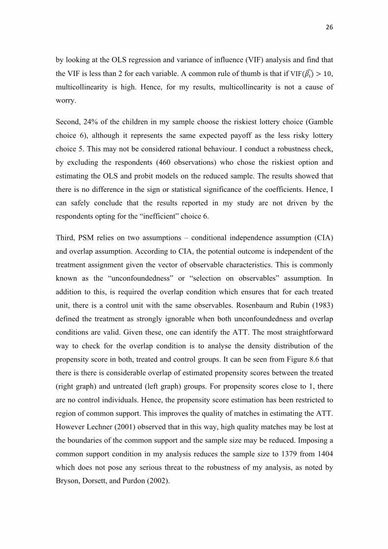
conditions are valid. Given these, one can identify the ATT. The most straightforward

way to check for the overlap condition is to analyse the density distribution of the

propensity score in both, treated and control groups. It can be seen from Figure 8.6 that

there is there is considerable overlap of estimated propensity scores between the treated

(right graph) and untreated (left graph) groups. For propensity scores close to 1, there

are no control individuals. Hence, the propensity score estimation has been restricted to

region of common support. This improves the quality of matches in estimating the ATT.

However Lechner (2001) observed that in this way, high quality matches may be lost at

the boundaries of the common support and the sample size may be reduced. Imposing a

common support condition in my analysis reduces the sample size to 1379 from 1404

which does not pose any serious threat to the robustness of my analysis, as noted by

Bryson, Dorsett, and Purdon (2002).

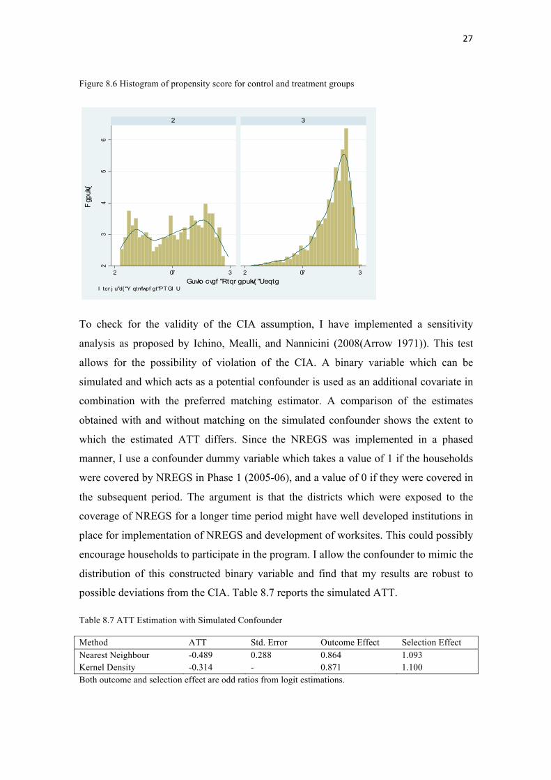
Figure 8.6 Histogram of propensity score for control and treatment groups

To check for the validity of the CIA assumption, I have implemented a sensitivity

analysis as proposed by Ichino, Mealli, and Nannicini (2008(Arrow 1971)). This test

allows for the possibility of violation of the CIA. A binary variable which can be

simulated and which acts as a potential confounder is used as an additional covariate in

combination with the preferred matching estimator. A comparison of the estimates

obtained with and without matching on the simulated confounder shows the extent to

which the estimated ATT differs. Since the NREGS was implemented in a phased

manner, I use a confounder dummy variable which takes a value of 1 if the households

were covered by NREGS in Phase 1 (2005-06), and a value of 0 if they were covered in

the subsequent period. The argument is that the districts which were exposed to the

coverage of NREGS for a longer time period might have well developed institutions in

place for implementation of NREGS and development of worksites. This could possibly

encourage households to participate in the program. I allow the confounder to mimic the

distribution of this constructed binary variable and find that my results are robust to

possible deviations from the CIA. Table 8.7 reports the simulated ATT.

Table 8.7 ATT Estimation with Simulated Confounder

Method ATT Std. Error Outcome Effect Selection Effect Nearest Neighbour -0.489 0.288 0.864 1.093 Kernel Density -0.314 - 0.871 1.100 Both outcome and selection effect are odd ratios from logit estimations.

23

45

6

2 07 3 2 07 3

2 3

Fgp

ukv{

Guvko cvgf "Rtqr gpukv{ "UeqtgI tcr j u"d{ "Y qtm"wpf gt"PTGI U

For the kernel density matching method, the simulated ATT is lower than that reported

in table 8.5. However, the deviation from baseline results is only 12%. Additionally, the

outcome and selection effects are also low. The nearest neighbour simulation is

conducted for only 1 nearest neighbour matching, and hence I cannot compare these to

the baseline results. This robustness check should be treated with caution – I cannot

conclusively rule out the possibility of “selection on unobservables” and that might

produce biased (upward bias) coefficient estimates for the ATT.

Lastly, in order to ensure the matching quality, one has to check that the distribution of

the covariates is balanced in both the control and treatment groups. There should be no

significant difference in the mean of the estimated propensity score between the

treatment and control group. This implies that additional conditioning on the

observables should not provide new information about the treatment decision. Table 8.8

reports the results of the two tests used to assess the matching quality – Standardised

bias test, and the t-Test. Standardised bias suggested by Rosenbaum and Rubin (1985) is

defined as the difference of the means between the treated and matched control

subsamples as a percentage of the square root of the average of sample variances in both

groups.

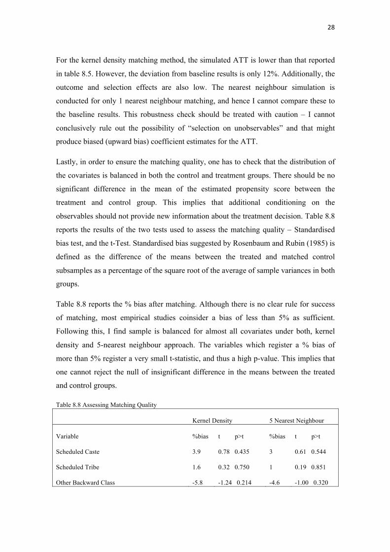
Table 8.8 reports the % bias after matching. Although there is no clear rule for success

of matching, most empirical studies coinsider a bias of less than 5% as sufficient.

Following this, I find sample is balanced for almost all covariates under both, kernel

density and 5-nearest neighbour approach. The variables which register a % bias of

more than 5% register a very small t-statistic, and thus a high p-value. This implies that

one cannot reject the null of insignificant difference in the means between the treated

and control groups.

Table 8.8 Assessing Matching Quality

Kernel Density 5 Nearest Neighbour

Variable %bias t p>t %bias t p>t

Scheduled Caste 3.9 0.78 0.435 3 0.61 0.544

Scheduled Tribe 1.6 0.32 0.750 1 0.19 0.851

Other Backward Class -5.8 -1.24 0.214 -4.6 -1.00 0.320

Parent's Education (Average Years) 3.5 0.91 0.364 5.5 1.45 0.146

Salaried Employee -1.2 -0.28 0.779 0.5 0.13 0.896

Main Source of Income : Agriculture 6.9 1.48 0.138 6.8 1.47 0.141

Hindu -1.8 -0.58 0.562 -2.1 -0.71 0.481

Muslim 1.8 0.55 0.581 2.2 0.67 0.500

Income from Pension 1.7 0.40 0.686 1.3 0.31 0.755

Income from Social Security (other than NREGS)

-7.8 -1.62 0.104 -3.5 -0.75 0.454

Participation in Indira Kranthi Patham (IKP) 1 0.21 0.830 3.8 0.85 0.393

Easily Raise Rs. 1000 -6.3 -1.34 0.180 -6.7 -1.42 0.155

Suffered Increase in Input Prices 0.7 0.15 0.881 0.6 0.13 0.899

Suffered Drought -4.7 -0.96 0.336 -2.8 -0.59 0.557

Suffered Crop Failure -1 -0.21 0.834 1.6 0.33 0.741

Suffered Livestock Death -1.5 -0.31 0.755 -3.7 -0.75 0.456

Housing Services Index 5.6 1.74 0.082 5.5 1.72 0.085

Consumer Durables Index -2.1 -0.47 0.636 0.1 0.03 0.980

IX. CONCLUSION

This paper examined the determinants of childhood risk aversion and found that

psychological factors, such as, death of a family member and inclusion in peer groups

play an important role in shaping risk attitudes. The results also highlight the

importance of socio-economic environment into which a child is born, as captured by

the wealth index, in shaping risk attitudes. 58% of the children who exhibit “risk

loving” tendencies come from households with an above mean wealth index (0.512).

The paper additionally studies the effectiveness of the NREGS in ensuring a safe and

stable environment for children, reflected in lower risk aversion. NREGS, being a

targeted program and harbouring self-selection among the eligible rural households,

poses serious econometric issues when studying the impact. However, this is overcome

by using a rich Young Lives panel data. Round 2 data with exhaustive information on

household level characteristic is used to conduct a propensity score matching analysis.

This is followed by studying the impact of the NREGS on the risk aversion behaviour in

children recorded in Round 3. NREGS reduced risk aversion in children by 36-43%.

The results from PSM are made robust, by conducting tests to ensure balancing, by

ensuring the validity of overlap condition, and by ensuring the validity of

unconfoundedness assumption through simulation model using confounder. The

NREGS have a significant negative impact on the risk aversion, that is, children

belonging to households covered under NREGS are able to partly correct for the

“accident” of birth and show signs of lower risk aversion.