Embed Size (px)
Citation preview

NPS Temporal Conference # 1

NPS Temporal Conference # 2
DESIGNING PANEL SURVEYSSPECIFICALLY RELEVANT TO NATIONAL PARKS
IN THE NORTHWEST
N. Scott UrquhartN. Scott UrquhartSenior Research ScientistSenior Research ScientistDepartment of StatisticsDepartment of Statistics
Colorado State UniversityColorado State UniversityFort Collins, CO 80527-1877Fort Collins, CO 80527-1877

NPS Temporal Conference # 3
INFERENCE PERSPECTIVES
Design BasedDesign Based Inferences rest on the probability structure
incorporated in the sampling plan Completely defensible; very minimal assumptions Limiting relative to using auxiliary information
Model AssistedModel Assisted Uses models to compliment underlying sampling
structure Has opportunities for use of auxiliary information
Model Based (eg: spatial statistics)Model Based (eg: spatial statistics) Ignores sampling plan Defensibility lies in defense of model

NPS Temporal Conference # 4
APPROACH OF THIS PRESENTATION
Use tools from the arena ofUse tools from the arena of Model assisted and Model based analyses
To study the performance of To study the performance of Design based & Model-assisted analyses
WHY?WHY? Without models,
performance evaluations need simulation
Before substantial data have been gatheredBefore substantial data have been gathered No basis for values to enter into simulation studies

NPS Temporal Conference # 5
STATUS & TRENDS OVER TIME STATUS & TRENDS OVER TIME IN ECOLOGICAL RESOURCES IN ECOLOGICAL RESOURCES
OF A REGIONOF A REGION
MAJOR POINTSMAJOR POINTS
STATUS & TRENDS OVER TIME STATUS & TRENDS OVER TIME IN ECOLOGICAL RESOURCES IN ECOLOGICAL RESOURCES
OF A REGIONOF A REGION
MAJOR POINTSMAJOR POINTS
Regional trend Regional trend site trend site trend Detection of trend requires substantial elapsed timeDetection of trend requires substantial elapsed time
Regional OR intensive site
Almost all indicators have substantial patterns inAlmost all indicators have substantial patterns intheir variabilitytheir variability
Design to capitalize on this; don’t fight it.
Minimize effect of site variability with planned Minimize effect of site variability with planned revisits – specific plans will be illustratedrevisits – specific plans will be illustrated
Design tradeoffs: TREND Design tradeoffs: TREND vs vs STATUSSTATUS

NPS Temporal Conference # 6
REGIONAL TREND REGIONAL TREND SITE TREND SITE TREND
The predominant theme of ecology:The predominant theme of ecology: Ecological processes How does a specific kind of ecosystem function
Energy flows Food webs Nutrient cycling
Most studies of such functions must be temporally Temporally intensive
– What material goes from where to where? Consequently spatially restrictive
In this situation: Temporal trend = site trend

NPS Temporal Conference # 7
REGIONAL TREND REGIONAL TREND SITE TREND SITE TREND( - CONTINUED)( - CONTINUED)
The predominant theme of ecologyThe predominant theme of ecologyversusversus
A Substantial (any) Agency Focus:A Substantial (any) Agency Focus: All of an ecological resource
In an area or region Across all of the variability present there
Most government regulations Apply to a whole area or region Only a few apply to specific sites The definition of a “region” certainly depends on what agency
makes the regulation

NPS Temporal Conference # 8
REGIONAL TREND REGIONAL TREND SITE TREND SITE TREND( - CONTINUED - III)( - CONTINUED - III)
The predominant theme of ecologyThe predominant theme of ecologyversusversus
A substantial agency (EPA) focus:A substantial agency (EPA) focus: An entire region, like
Lakes in the Adirondack Mountains All lakes in Northeastern US All (wadeable) streams the mid-Appalachian Mountains
Or National Park ServiceOr National Park Service All riparian areas in Olympic National Park All riparian areas in National Parks in the
coastal Northwest

NPS Temporal Conference # 9
TREND ACROSS TIME - What is it?
Any response which changes across time in a Any response which changes across time in a generally generally
Increasing or Decreasing
Manner shows trendManner shows trend Monotonic change is not essential.
If trend of this sort is present, If trend of this sort is present, it will be detectable as linear trend.it will be detectable as linear trend.
This does NOTNOT mean trend must be linear (examples follow)
Any specified form is detectable Time = years, here

NPS Temporal Conference # 10
TREND ACROSS TIME - What is it?(continued)
TREND = YES
50
70
90
1989 1991 1993 1995
Year
TREND = NO; PATTERN = YES
50
70
90
1989 1991 1993 1995 1997
Year
TREND = YES, PATTERN = YES
0
50
100
150
200
250
300
350
400
1955 1965 1975 1985 1995 2005
YEAR
CA
RB
ON
DIO
XID
E
CO
NC
EN
TR
AT
ION
(p
pm
)
TREND = NO; PATTERN = YES
0
50
100
150
200
250
300
350
1955 1965 1975 1985 1995 2005
YEAR
CA
RB
ON
DIO
XID
E
CO
NC
EN
TR
AT
ION
(p
pm
)

NPS Temporal Conference # 11
TREND = NO; PATTERN = YES
0
50
100
150
200
250
300
350
1955 1965 1975 1985 1995
YEAR
DE
TR
EN
DE
D C
AR
BO
N D
IOX
IDE
C
ON
CE
NT
RA
TIO
N (
pp
m)

NPS Temporal Conference # 12
TREND DETECTION REQUIRES TREND DETECTION REQUIRES SUBSTANTIAL ELAPSED TIMESUBSTANTIAL ELAPSED TIME
IT IS NEARLY IMPOSSIBLE TO DETECT IT IS NEARLY IMPOSSIBLE TO DETECT TREND IN LESS THAN FIVE YEARS. WHY?TREND IN LESS THAN FIVE YEARS. WHY?
vart ti
( )( )
2
2
( )t ti 2

NPS Temporal Conference # 13
BIOLOGICAL INDICATORS HAVE SOMEWHAT BIOLOGICAL INDICATORS HAVE SOMEWHAT MORE VARIABILITY THAN PHYSICAL MORE VARIABILITY THAN PHYSICAL INDICATORS – BUT THIS VARIES, TOOINDICATORS – BUT THIS VARIES, TOO
Subsequent slides show the relative amount of Subsequent slides show the relative amount of variability variability
Ordered by the amount of residual variability: least to most (aquatic responses)
Acid Neutralizing CapacityAcid Neutralizing Capacity Ln(Conductance)Ln(Conductance) Ln(Chloride)Ln(Chloride) pH(Closed system)pH(Closed system) Secchi DepthSecchi Depth Ln(Total Nitrogen)Ln(Total Nitrogen) Ln(Total Phosphorus)Ln(Total Phosphorus) Ln(Chlorophyll A)Ln(Chlorophyll A) Ln( # zooplankton taxa)Ln( # zooplankton taxa) Ln( # rotifer taxa)Ln( # rotifer taxa) Maximum TemperatureMaximum Temperature
And others, both aquatic and terrestrial

NPS Temporal Conference # 14
POPULATION VARIANCE: POPULATION VARIANCE:
YEAR VARIANCE:YEAR VARIANCE:
RESIDUAL VARIANCE:RESIDUAL VARIANCE:
2( )SITE
2( )YEAR
IMPORTANT COMPONENTS OF VARIANCEIMPORTANT COMPONENTS OF VARIANCE
2( )RESIDUAL

NPS Temporal Conference # 15
POPULATION VARIANCE: POPULATION VARIANCE:
Variation among values of an indicator (response) across all sites in a park or group of related parks, that is, across a population or subpopulation of sites
2( )SITE
IMPORTANT COMPONENTS OF VARIANCEIMPORTANT COMPONENTS OF VARIANCE( - CONTINUED)( - CONTINUED)

NPS Temporal Conference # 16
YEAR VARIANCE: YEAR VARIANCE:
Concordant variation among values of an indicator (response) across years for ALLALL sites in a regional population or subpopulation
NOT variation in an indicator across years at a single site
Detrended remainder, if trend is present Effectively the deviation away from the trend line (or other
curve)
2( )YEAR
IMPORTANT COMPONENTS OF VARIANCEIMPORTANT COMPONENTS OF VARIANCE( - CONTINUED II)( - CONTINUED II)

NPS Temporal Conference # 17
Residual component of varianceResidual component of variance
Has several contributors
Year*Site interaction This contains most of what ecologists would call year to year
variation, i.e. the site specific part
Index variation Measurement error Crew-to-crew variation (minimize with documented protocols
and training) Local spatial = protocol variation Short term temporal variation
IMPORTANT COMPONENTS OF VARIANCEIMPORTANT COMPONENTS OF VARIANCE( - CONTINUED - III)( - CONTINUED - III)
2( )RESIDUAL

NPS Temporal Conference # 18
SOURCE OF DATA FOR ESTIMATES OF COMPONENTS OF VARIANCE
EMAP Surface Waters: EMAP Surface Waters: Northeast Lakes Pilot 1991 - 1994 Northeast Lakes Pilot 1991 - 1994
About 450 observationsAbout 450 observations Over four years Including about 350 distinct lakes Design allowed estimation of several residual
components

NPS Temporal Conference # 19
COMPOSITION OF TOTAL VARIANCE - NE LAKES
0.00 0.20 0.40 0.60 0.80 1.00
Maximum Temperature
Ln( # rotifer taxa)
Ln( # zooplankton taxa)
Ln(Chlorophyll A)
Ln(Total Phosphorus)
Ln(Total Nitrogen)
Secchi Depth
pH(Closed system)
Ln(Chloride)
Ln(Conductance)
Acid Neutralizing Capacity
PROPORTION OF VARIANCE
RESIDUAL COMPONENT OF VARIANCE
LAKE COMPONENT OF VARIANCE
YEAR

NPS Temporal Conference # 20
SOURCE OF COMPONENTS OF VARIANCE FROM NW HABITAT
Oregon Department of Fisheries and Wildlife – stream habitat surveyOregon Department of Fisheries and Wildlife – stream habitat surveyGRADIENT: Stream gradient measured on siteWIDTH: Wetted stream widthACW: Active Channel ACH: Active Channel HeightUNITS100: Number of distinct habitat units per 100 meters of stream length NOPOOLS: Number of pools in the surveyed reachPOOLS100: Number of pools per 100 metersPCTPOOL: % of reach length in poolsPCTFINES: % stream substrate that is sand or finer particle sizePCTGRAVEL: % of stream stubstrate that is gravel sized particlesRIFSNDOR: % of riffle stream length that is sand or finer particle sizeRIFGRAV: % of riffle stream length that is gravel sized particlesSHADE: % stream channel shadedLOG(PIECESLWD +0.01): Number of pieces of large woody debris per 100
meters.LOG(VOLUMELWD +0.01): Volume of large woody debris (m^3/100 meters)RESIDPD: Volume of residual pools (pools remaining if streamflow stopped)

NPS Temporal Conference # 21
COMPOSITION OF TOTAL VARIANCE NW HABITAT
0.00 0.10
Gradient
Active Channel Width
UNITS100
Pools per 100m
% Fines
% Riffle fine
% Shaded
LOG(VOLUME L WD)
pH(Closed system)
Ln(Conductance)
PROPORTION OF VARIANCE
RESIDUAL COMPONENT OF VARIANCE
LAKE COMPONENT OF VARIANCE
YEAR

NPS Temporal Conference # 22
SOURCE OF COMPONENTS OF VARIANCE FROM GRAND CANYON
Grand Canyon Monitoring and Research CenterGrand Canyon Monitoring and Research Center Effects of Glen Canyon Dam on the near River Habitat
in the Grand Canyon At various heights above the river Height is measured as the height of the river’s water
at various flow rates Eg: 15K cfs, 25K cfs, 35K cfs, 45K cfs & 60K cfs
Using first two years’ dataUsing first two years’ data Mike Kearsley – UNA
Design = spatially balancedDesign = spatially balanced With about 1/3 revisited

NPS Temporal Conference # 23
COMPOSITION OF TOTAL VARIANCEGRAND CANYON -- NEAR RIVER VEGETATION
0.00 0.20 0.40 0.60 0.80 1.00
Veg - 25K cfs
Veg - 35K cfs
Veg - 45K cfs
Veg - 60K cfs
Richness - 15K cfs
Richness - 25K cfs
Richness - 35K cfs
Richness - 45K cfs
Richness - 60K cfs
PROPORTION OF VARIANCE
RESIDUAL COMPONENT OF VARIANCE
SITE COMPONENT OF VARIANCELAKE COMPONENT
YEAR

NPS Temporal Conference # 24
ALL VARIABILITY IS OF INTERESTALL VARIABILITY IS OF INTEREST
The site component of variance is one of the major The site component of variance is one of the major descriptors of the regional populationdescriptors of the regional population
The year component of variance often is small to The year component of variance often is small to small to estimate. It is a major enemy for detecting small to estimate. It is a major enemy for detecting trend over time.trend over time.
If it has even a moderate size, “sample size” reverts to the number of years.
In this case, the number of visits and/or number of sites has no practical effect.

NPS Temporal Conference # 25
ALL VARIABILITY IS OF INTERESTALL VARIABILITY IS OF INTEREST( - CONTINUED)( - CONTINUED)
Residual variance characterizes the inherent Residual variance characterizes the inherent variation in the response or indicator.variation in the response or indicator.
But some of its subcomponents may contain useful But some of its subcomponents may contain useful management informationmanagement information
CREW EFFECTS ===> training VISIT EFFECTS ===> need to reexamine definition of
index (time) window or evaluation protocol MEASUREMENT ERROR ===> work on
laboratory/measurement problems

NPS Temporal Conference # 26
DESIGN TRADE-OFFS: TREND DESIGN TRADE-OFFS: TREND vs vs STATUSSTATUS
How do we detect trend in spite of all of this How do we detect trend in spite of all of this variation?variation?
Recall two old statistical “friends.”Recall two old statistical “friends.” Variance of a mean, and Blocking

NPS Temporal Conference # 27
DESIGN TRADE-OFFS: TREND DESIGN TRADE-OFFS: TREND vs vs STATUSSTATUS( - CONTINUED)( - CONTINUED)
VARIANCE OF A MEAN:VARIANCE OF A MEAN:
Where m members of the associated population have been randomly selected and their response values averaged.
Here the “mean” is a regional average slope, so "2" refers to the variance of an estimated slope ---
var meanm
( ) 2

NPS Temporal Conference # 28
DESIGN TRADE-OFFS: TREND DESIGN TRADE-OFFS: TREND vs vs STATUSSTATUS( - CONTINUED - II)( - CONTINUED - II)
ConsequentlyConsequently
BecomesBecomes
Note that the regional averaging of slopes has the Note that the regional averaging of slopes has the same effect as continuing to monitor at one site for a same effect as continuing to monitor at one site for a much longer time period.much longer time period.
var meanm
( ) 2
var regional mean slopem t ti
( )( )
1 2
2

NPS Temporal Conference # 29
DESIGN TRADE-OFFS: TREND DESIGN TRADE-OFFS: TREND vs vs STATUSSTATUS( - CONTINUED - III)( - CONTINUED - III)
Now, Now, 22, in total, is large., in total, is large.
If we take one regional sample of sites at one time, If we take one regional sample of sites at one time, and another at a subsequent time, the site and another at a subsequent time, the site component of variance is included in component of variance is included in 22..
Enter the concept of blocking, familiar from Enter the concept of blocking, familiar from experimental design.experimental design.
Regard a site like a block Periodically revisit a site The site component of variance vanishes from the
variance of a slope.

NPS Temporal Conference # 30
NOW PUT IT ALL TOGETHER
Question: “ What kind of temporal design should Question: “ What kind of temporal design should you use for Northwest National Parks?you use for Northwest National Parks?
We’ll investigate two (families) of recommended We’ll investigate two (families) of recommended designs.designs.
All illustrations will be based on 30 site visits per year, as Andrea recommended.
General relations are uninfluenced by number of sites visited per year, but specific performance is.
We’ll use the panel notation Trent set out.We’ll use the panel notation Trent set out.

NPS Temporal Conference # 31
RECOMMENDATION OF FULLER and BREIDT
Based on the Natural Resources Inventory (NRI)Based on the Natural Resources Inventory (NRI) Iowa State & US Department of Agriculture
Oriented toward soil erosion & Changes in land use
Their recommendationTheir recommendation Pure panel = [1-0] = “Always Revisit” Independent = [1-n] = “Never Revisit”
Evaluation contextEvaluation context No trampling effect – remotely sensed data No year effects
Administrative reality of potential variation in Administrative reality of potential variation in funding from year to yearfunding from year to year
MATH RECOME… 100% 50% 0% 50%

NPS Temporal Conference # 32
TEMPORAL LAYOUT OF [(1-0), (1-n)]YEARYEAR 11 22 33 44 55 66 77 88 99 1010 1111 1212 1313 1414 1515 1616 1717 1818 1919 2020
[1-0][1-0] XX XX XX XX XX XX XX XX XX XX XX XX XX XX XX XX XX XX XX XX
[1-n][1-n] XX
XX
XX
XX
XX
XX
XX
XX
XX
XX
XX
XX
XX
XX
XX
XX
XX
XX
XX
XX

NPS Temporal Conference # 33
FIRST TEMPORAL DESIGN FAMILY
30 site visits per year30 site visits per year
[1-0][1-0] 3030 2020 1010 00
[1-n][1-n] 00 1010 2020 3030
ALWAYSALWAYS
REVISITREVISIT
NEVERNEVER
REVISITREVISIT

NPS Temporal Conference # 34
POWER TO DETECT TREND
FIRST TEMPORAL DESIGN FAMILY NO YEAR EFFECT
0
0.2
0.4
0.6
0.8
1
0 5 10 15 20
YEARS
PO
WE
R
30:020:1010:200:30
Always Revisit
Never Revisit

NPS Temporal Conference # 35
POWER TO DETECT TREND
FIRST TEMPORAL DESIGN FAMILY, MODEST (= SOME) YEAR EFFECT
0
0.2
0.4
0.6
0.8
1
0 5 10 15 20
YEARS
PO
WE
R
30:020:1010:200:30

NPS Temporal Conference # 36
POWER TO DETECT TREND
FIRST TEMPORAL DESIGN FAMILYBIG (= LOTS) YEAR EFFECT
0
0.2
0.4
0.6
0.8
1
0 5 10 15 20
YEARS
PO
WE
R
30:020:1010:200:30

NPS Temporal Conference # 37
FOREST INVENTORY ANALYSIS (FIA) HAS A SYSTEMATIC SPATIAL DESIGN
WITH [1-9]
Doesn’t match up well with [1-0] and [1-n]Doesn’t match up well with [1-0] and [1-n] We need to investigate alternativesWe need to investigate alternatives
YEARYEAR 11 22 33 44 55 66 77 88 99 1010 1111 1212 1313 1414 1515 1616 1717 1818 1919 2020 2121
FIAFIA XX XX XX

NPS Temporal Conference # 38
SERIALLY ALTERNATING TEMPORAL DESIGN [(1-3)4 ] SOMETIMES USED BY
EMAP
YEARYEAR 11 22 33 44 55 66 77 88 99 1010 1111 1212 1313 1414 1515 1616 1717 1818 1919 2020 2121
FIAFIA XX XX XX
[(1-3)[(1-3)4 4 ]] XX XX XX XX XX XX
XX XX XX XX XX
XX XX XX XX XX
XX XX XX XX XX

NPS Temporal Conference # 39
SERIALLY ALTERNATING TEMPORAL DESIGN [(1-3)4 ] SOMETIMES USED BY
EMAP
YEARYEAR 11 22 33 44 55 66 77 88 99 1010 1111 ……
FIAFIA XX XX
[(1-3)[(1-3)4 4 ]] XX XX XX ……
XX XX XX ……
XX XX XX ……
XX XX ……
Unconnected in an experimental design senseUnconnected in an experimental design sense Very weak design for estimating year effects, if present

NPS Temporal Conference # 40
SPLIT PANEL [(1-4)5 , --- ]
YEARYEAR 11 22 33 44 55 66 77 88 99 1010 1111 1212 1313 1414 1515 1616 1717 1818 1919 2020 2121
FIAFIA XX XX XX
[(1-4)[(1-4)5 5 ]] XX XX XX XX XX
XX XX XX XX
XX XX XX XX
XX XX XX XX
XX XX XX XX
AGAIN, Unconnected in an experimental design AGAIN, Unconnected in an experimental design sensesense Matches better with FIA Still a very weak design for estimating year effects, if
present

NPS Temporal Conference # 41
SPLIT PANEL [(1-4)5 ,(2-3)5 ]
This Temporal Design IS connectedThis Temporal Design IS connectedHas three panels which match up with FIAHas three panels which match up with FIA
YEARYEAR 11 22 33 44 55 66 77 88 99 1010 1111 1212 1313 1414 1515 1616 1717 1818 1919 2020 2121
FIAFIA XX XX XX
[(1-4)[(1-4)5 5 ]] XX XX XX XX XX
XX XX XX XX
XX XX XX XX
XX XX XX XX
XX XX XX XX
[(2-3)[(2-3)5 5 ]] XX XX XX XX XX XX XX XX XX
XX XX XX XX XX XX XX XX
XX XX XX XX XX XX XX XX
XX XX XX XX XX XX XX XX
XX XX XX XX XX XX XX XX

NPS Temporal Conference # 42
SECOND TEMPORAL DESIGN FAMILY
30 site visits per year30 site visits per year
[1-4][1-4] 3030 2020 1010 00
[2-3][2-3] 00 55 1010 1515

NPS Temporal Conference # 43
POWER TO DETECT TREND
SECOND TEMPORAL DESIGN FAMILY NO YEAR EFFECT
0
0.2
0.4
0.6
0.8
1
0 5 10 15 20
YEARS
PO
WE
R
30:020:5
10:10 0:15

NPS Temporal Conference # 44
POWER TO DETECT TREND
SECOND TEMPORAL DESIGN FAMILYSOME YEAR EFFECT
0
0.2
0.4
0.6
0.8
1
0 5 10 15 20
YEARS
PO
WE
R
30:020:5
10:10 0:15

NPS Temporal Conference # 45
POWER TO DETECT TREND
SECOND TEMPORAL DESIGN FAMILYLOTS OF YEAR EFFECT
0
0.2
0.4
0.6
0.8
1
0 5 10 15 20
YEARS
PO
WE
R
30:020:5
10:10 0:15

NPS Temporal Conference # 46
COMPARISON OF POWER TO DETECT TRENDDESIGN 1 & 2 = ROWS
0
0.2
0.4
0.6
0.8
1
0 5 10 15 20
YEARS
PO
WE
R
0
0.2
0.4
0.6
0.8
1
0 5 10 15 20
YEARS
PO
WE
R
0
0.2
0.4
0.6
0.8
1
0 5 10 15 20
YEARS
PO
WE
R
0
0.2
0.4
0.6
0.8
1
0 5 10 15 20
YEARS
PO
WE
R
0
0.2
0.4
0.6
0.8
1
0 5 10 15 20
YEARS
PO
WE
R
0
0.2
0.4
0.6
0.8
1
0 5 10 15 20
YEARS
PO
WE
R
YEAR EFFECT
NONE SOME LOTS

NPS Temporal Conference # 47
POWER TO DETECT TREND
VARYING YEAR EFFECT AND TEMPORAL DESIGN
0
0.2
0.4
0.6
0.8
1
0 5 10 15 20
YEARS
PO
WE
R
TEMPORAL DESIGN 2
TEMPORAL DESIGN 1NONE
SOME
LOTS

NPS Temporal Conference # 48
STANDARD ERROR OF STATUS
TEMPORAL DESIGN 1, NO YEAR EFFECT
0
0.1
0.2
0.3
0.4
0.5
0 5 10 15 20
YEARS
SE
ST
AT
US
30:0 20:10 10:20 0:30
TOTAL OF 30 SITES
110 SITES VISITED BY
YEAR 5 410 SITES VISITED BY
YEAR 20

NPS Temporal Conference # 49
STANDARD ERROR OF STATUS
TEMPORAL DESIGN 1, SOME YEAR EFFECT
0
0.1
0.2
0.3
0.4
0.5
0 5 10 15 20
YEARS
SE
ST
AT
US
30:0 20:10 10:20 0:30

NPS Temporal Conference # 50
STANDARD ERROR OF STATUS
TEMPORAL DESIGN 1, LOTS OF YEAR EFFECT
0
0.1
0.2
0.3
0.4
0.5
0 5 10 15 20
YEARS
SE
ST
AT
US
30:0 20:10 10:20 0:30

NPS Temporal Conference # 51
STANDARD ERROR OF STATUS
TEMPORAL DESIGN 2, NO YEAR EFFECT
0
0.1
0.2
0.3
0.4
0.5
0 5 10 15 20
YEARS
SE
ST
AT
US
30:020:5
10:10 0:15
TOTAL OF 150 SITES
TOTAL OF 75 SITES

NPS Temporal Conference # 52
STANDARD ERROR OF STATUS
TEMPORAL DESIGN 2, SOME YEAR EFFECT
0
0.1
0.2
0.3
0.4
0.5
0 5 10 15 20
YEARS
SE
ST
AT
US
30:020:5
10:10 0:15

NPS Temporal Conference # 53
STANDARD ERROR OF STATUS
TEMPORAL DESIGN 2, LOTS OF YEAR EFFECT
0
0.1
0.2
0.3
0.4
0.5
0 5 10 15 20
YEARS
SE
ST
AT
US
30:020:5
10:10 0:15

NPS Temporal Conference # 54
SO WHAT?
Regardless of evaluation circumstances,Regardless of evaluation circumstances, Trend detection improves the more the same sites are
revisited Status estimation improves as the number of distinct sites
visited increases
Temporal design 2 is better than temporal design 1 in Temporal design 2 is better than temporal design 1 in relevant casesrelevant cases Its power is only slightly influenced by split between panels

NPS Temporal Conference # 55
METADATA
Really important for your successorsReally important for your successors Like your grandchildrens’ generation
I’ll comment about this later in the conference if you I’ll comment about this later in the conference if you want me towant me to

NPS Temporal Conference # 56
This research is funded by
U.S.EPA – Science To AchieveResults (STAR) ProgramCooperativeAgreement
# CR - 829095
The work reported here today was developed under the STAR Research Assistance Agreement CR-829095 awarded by the U.S. Environmental Protection Agency (EPA) to Colorado State University. This presentation has not been formally reviewed by EPA. The views expressed here are solely those of presenter and STARMAP, the Program he represents. EPA does not endorse any products or commercial services mentioned in this presentation.
FUNDING ACKNOWLEDGEMENT

NPS Temporal Conference # 57
TEMPORAL DESIGN 1ALWAYS REVISIT
TIME PERIOD ( ex: YEARS)PANEL 1 2 3 4 5 6 7 8 9 10 11 12 13 ...
1 X X X X X X X X X X X X X

NPS Temporal Conference # 58
TEMPORAL DESIGN 2:
NEVER REVISIT
TIME PERIOD ( ex: YEARS)PANEL 1 2 3 4 5 6 7 8 9 10 11 12 13 ... 1 X 2 X 3 X 4 X 5 X 6 X 7 X 8 X 9 X
NPS Temporal Conference # 59
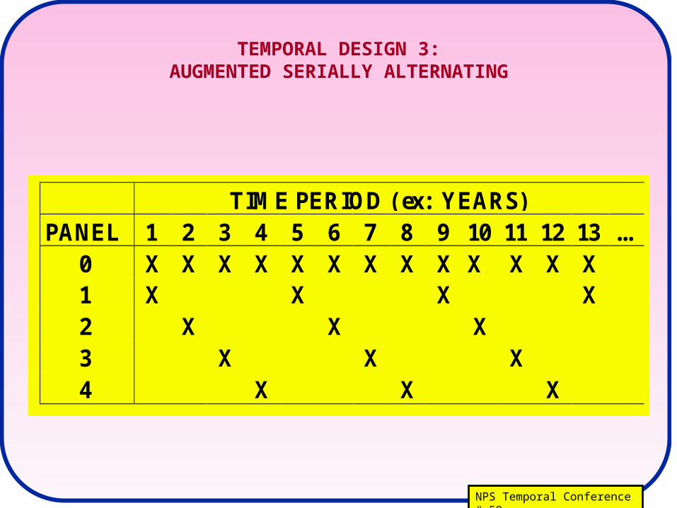
TEMPORAL DESIGN 3:AUGMENTED SERIALLY ALTERNATING
TIME PERIOD ( ex: YEARS)PANEL 1 2 3 4 5 6 7 8 9 10 11 12 13 ... 0 X X X X X X X X X X X X X 1 X X X X 2 X X X 3 X X X 4 X X X

NPS Temporal Conference # 60
TEMPORAL DESIGN 4: SPLIT PANEL
SERIALLY ALTERNATINGPLUS SERIALLY ALTERNATING WITH CONSECUTIVE YEAR REVISITS
TIME PERIOD ( ex: YEARS)PANEL 1 2 3 4 5 6 7 8 9 10 11 12 13 ... 1 X X X X 1A X X X X X X X 2 X X X 2A X X X X X X 3 X X X 3A X X X X X X 4 X X X 4A X X X X X X

NPS Temporal Conference # 61
DESIGN EFFECT
0
0.2
0.4
0.6
0.8
1
0 5 10 15 20TIME ( = YEARS )
PO
WE
R f
or
TR
EN
D
DESIGNS 1, 3, & 4
DESIGN 2
A

NPS Temporal Conference # 62
LAKE EFFECT; DESIGNS 2 & 4VAR LAKE = 1, 2, 5
0
0.2
0.4
0.6
0.8
1
0 5 10 15 20
TIME ( = YEARS )
PO
WE
R f
or
TR
EN
D
DESIGN 4ALL VARIANCES
DESIGN 2LAKE VAR = 5
1
2
B

NPS Temporal Conference # 63
YEAR EFFECT - DESIGNS 2 & 4
0
0.2
0.4
0.6
0.8
1
0 5 10 15 20
TIME ( = YEARS )
PO
WE
R f
or
TR
EN
D
DESIGN 2
DESIGN 4
YEAR EFFECT0, 0.05, 0.10
TOP CURVES FOR 0.00
C

NPS Temporal Conference # 64
STANDARD ERROR OF ESTIMATED STATUS -ALL DESIGNS
0
0.2
0.4
0 5 10 15 20
TIME ( =Years )
ST
AN
DA
RD
ER
RO
R (
ST
AT
US
)
DESIGN 1
DESIGN 2
DESIGNS 3 & 4
D

NPS Temporal Conference # 65
SIZE OF TREND EFFECT: DESIGN 4
0
0.2
0.4
0.6
0.8
1
0 5 10 15 20
TIME ( = YEARS )
PO
WE
R f
or
TR
EN
D = 0.03 = 0.02
= 0.015
= 0.01
E

NPS Temporal Conference # 66
SAMPLE SIZE EFFECT - DESIGN 4
0
0.2
0.4
0.6
0.8
1
0 5 10 15 20TIME ( = YEARS )
PO
WE
R f
or
TR
EN
D
n = 240
n = 120
n = 60
F

NPS Temporal Conference # 67
SECCHI DEPTH
0
0.2
0.4
0.6
0.8
1
1.2
0 5 10 15 20
TIME ( = YEARS )
PO
WE
R f
or
TR
EN
D
A
1% PER YEAR3% PER YEAR

NPS Temporal Conference # 68
ln ( CHLOROPHYLL a )
0
0.2
0.4
0.6
0.8
1
0 5 10 15 20
TIME ( = YEARS )
PO
WE
R f
or
TR
EN
D
A
1% PER YEAR
3% PER YEAR
NPS Temporal Conference # 69
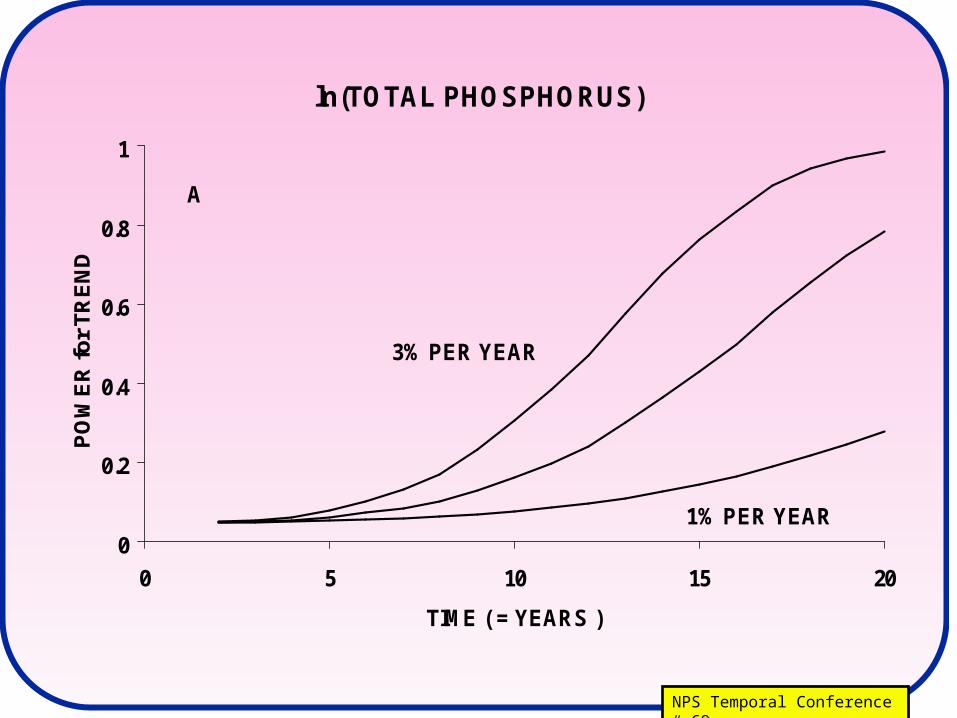
ln(TOTAL PHOSPHORUS)
0
0.2
0.4
0.6
0.8
1
0 5 10 15 20
TIME ( = YEARS )
PO
WE
R f
or
TR
EN
D
A
1% PER YEAR
3% PER YEAR

NPS Temporal Conference # 70
ln( NUMBER ZOOPLANKTON TAXA)
0
0.2
0.4
0.6
0.8
1
0 5 10 15 20
TIME ( = YEARS )
PO
WE
R f
or
TR
EN
D
1% PER YEAR
3% PER YEAR