Now we focus on discrete random variables. We will look at these in general, including calculating the mean and standard deviation. Then we will look more in depth at binomial random variables which are a special type of discrete random variable with many applications in practice. 

In the introduction, we stated that a random variable assigns a unique numeric value to the outcome of a random experiment and we defined discrete random variables as having a countable number of possible values. There may be an infinite number of possible values (in the sense that we do not know the potential maximum) but there are always gaps between the possible values. 

We use probability distributions to represent the distribution of a discrete random variable. 

What do we mean by a probability distribution? This is similar to frequency distributions except frequency distributions summarize data for one categorical variable and now we have a discrete random variable which will always represent a number and we are thinking about it theoretically – what if we were to repeat this experiment infinitely many times? 

1

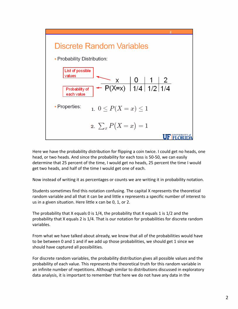
Here we have the probability distribution for flipping a coin twice. I could get no heads, one head, or two heads. And since the probability for each toss is 50‐50, we can easily determine that 25 percent of the time, I would get no heads, 25 percent the time I would get two heads, and half of the time I would get one of each. 

Now instead of writing it as percentages or counts we are writing it in probability notation. 

Students sometimes find this notation confusing. The capital X represents the theoretical random variable and all that it can be and little x represents a specific number of interest to us in a given situation. Here little x can be 0, 1, or 2. 

The probability that X equals 0 is 1/4, the probability that X equals 1 is 1/2 and the probability that X equals 2 is 1/4. That is our notation for probabilities for discrete random variables. 

From what we have talked about already, we know that all of the probabilities would have to be between 0 and 1 and if we add up those probabilities, we should get 1 since we should have captured all possibilities. 

For discrete random variables, the probability distribution gives all possible values and the probability of each value. This represents the theoretical truth for this random variable in an infinite number of repetitions. Although similar to distributions discussed in exploratory data analysis, it is important to remember that here we do not have any data in the 

2

traditional sense. 

2

We can use these probability distributions to answer questions of interest by taking, and possibly combining, the probabilities of interest from the probability distribution. 

In this table, we are assuming we have a discrete random variable that can take on the values of 0, 1, 2, 3, 4, or 5 and we are providing common keywords for questions involving probabilities of discrete random variables. We might ask questions such as what is the probability that X is "no less than 2." What that really means is: "2 or more," which I could write in notation as "greater than or equal to 2." Because it is discrete and it stops at five that means 2, 3, 4, or 5. 

Return to this table if you need to verify the correct interpretation for a particular problem. 

Be aware that this is only for discrete random variables – this table does not work for continuous random variables since for continuous random variables, there are no gaps and we cannot list the possible values as we can here for discrete random variables. 

3

The examples in the online materials will give additional examples. We will illustrate probability distributions using two scenarios. We call them Example A and Example B. 

For Example A, we will suppose that 8% of US adults aged 20 and over have diabetes. We could also say diabetes has a prevalence of 8% among this population. 

Suppose we select n people at random from this population. Here are some of the questions we will learn to answer. • How many would we expect to have diabetes? The word "expect" is the average, the 

mean, where would the center be? If I looked at all of the possibilities, how many would I expect, on average, to have diabetes? 

• What is the probability that none of them will have diabetes? At least one (that's a little trick). 

• What's the distribution of this whole random variable X? What does its whole picture look like? 

• How variable is this whole random variable X? 

Once we start getting a picture of the distribution in theory then we can answer all of these questions easily. 

4

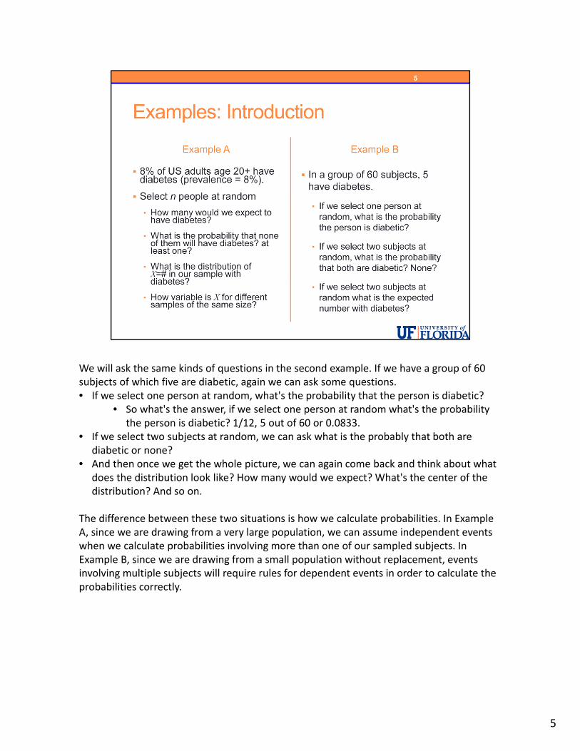
We will ask the same kinds of questions in the second example. If we have a group of 60 subjects of which five are diabetic, again we can ask some questions. • If we select one person at random, what's the probability that the person is diabetic? 

• So what's the answer, if we select one person at random what's the probability the person is diabetic? 1/12, 5 out of 60 or 0.0833. 

• If we select two subjects at random, we can ask what is the probably that both are diabetic or none? 

• And then once we get the whole picture, we can again come back and think about what does the distribution look like? How many would we expect? What's the center of the distribution? And so on. 

The difference between these two situations is how we calculate probabilities. In Example A, since we are drawing from a very large population, we can assume independent events when we calculate probabilities involving more than one of our sampled subjects. In Example B, since we are drawing from a small population without replacement, events involving multiple subjects will require rules for dependent events in order to calculate the probabilities correctly. 

5

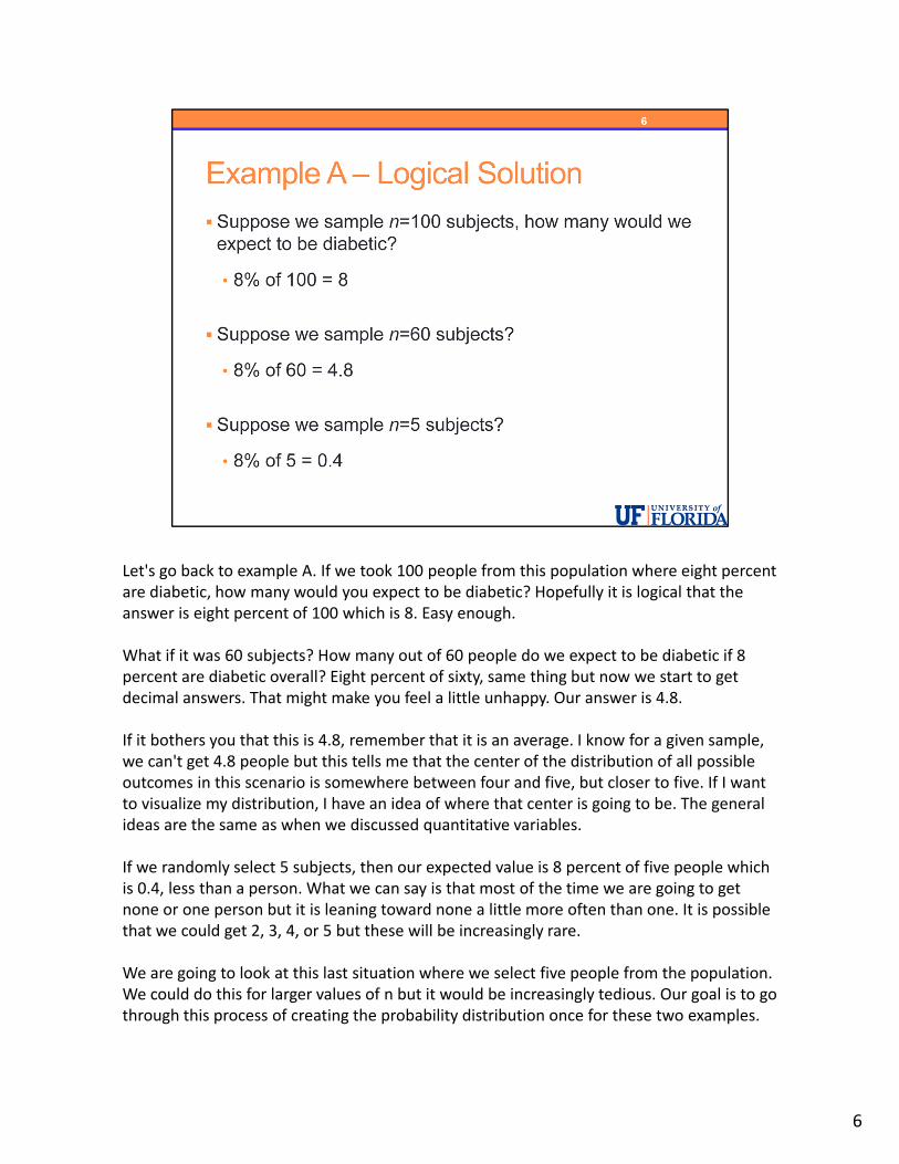
Let's go back to example A. If we took 100 people from this population where eight percent are diabetic, how many would you expect to be diabetic? Hopefully it is logical that the answer is eight percent of 100 which is 8. Easy enough. 

What if it was 60 subjects? How many out of 60 people do we expect to be diabetic if 8 percent are diabetic overall? Eight percent of sixty, same thing but now we start to get decimal answers. That might make you feel a little unhappy. Our answer is 4.8. 

If it bothers you that this is 4.8, remember that it is an average. I know for a given sample, we can't get 4.8 people but this tells me that the center of the distribution of all possible outcomes in this scenario is somewhere between four and five, but closer to five. If I want to visualize my distribution, I have an idea of where that center is going to be. The general ideas are the same as when we discussed quantitative variables. 

If we randomly select 5 subjects, then our expected value is 8 percent of five people which is 0.4, less than a person. What we can say is that most of the time we are going to get none or one person but it is leaning toward none a little more often than one. It is possible that we could get 2, 3, 4, or 5 but these will be increasingly rare. 

We are going to look at this last situation where we select five people from the population. We could do this for larger values of n but it would be increasingly tedious. Our goal is to go through this process of creating the probability distribution once for these two examples. 

6

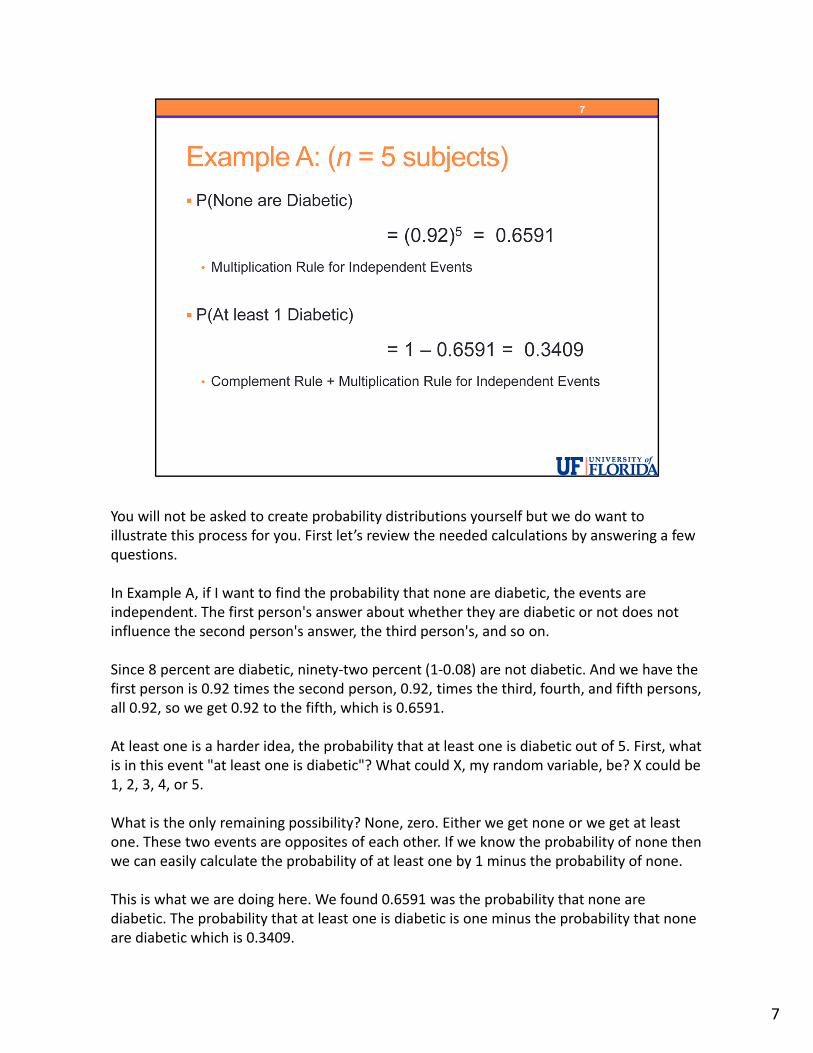
You will not be asked to create probability distributions yourself but we do want to illustrate this process for you. First let’s review the needed calculations by answering a few questions. 

In Example A, if I want to find the probability that none are diabetic, the events are independent. The first person's answer about whether they are diabetic or not does not influence the second person's answer, the third person's, and so on. 

Since 8 percent are diabetic, ninety‐two percent (1‐0.08) are not diabetic. And we have the first person is 0.92 times the second person, 0.92, times the third, fourth, and fifth persons, all 0.92, so we get 0.92 to the fifth, which is 0.6591. 

At least one is a harder idea, the probability that at least one is diabetic out of 5. First, what is in this event "at least one is diabetic"? What could X, my random variable, be? X could be 1, 2, 3, 4, or 5. 

What is the only remaining possibility? None, zero. Either we get none or we get at least one. These two events are opposites of each other. If we know the probability of none then we can easily calculate the probability of at least one by 1 minus the probability of none. 

This is what we are doing here. We found 0.6591 was the probability that none are diabetic. The probability that at least one is diabetic is one minus the probability that none are diabetic which is 0.3409. 

7

We are also reminding you which basic probability rules we are applying here. For the first, the multiplication rule for independent events. 

For the second, we applied the multiplication rule for independent events to get 0.6591 and then we used the compliment rule to get back to at least one. 

We are heading towards binomial random variables but first we are spending a little bit of time talking about general discrete random variables. 

Now we will look at creating the entire probability distribution for Example A where we have taken a sample of 5 subjects from our population of all US adults age 20+ in which 8 percent are diabetic. 

8

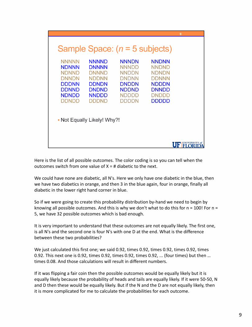
Here is the list of all possible outcomes. The color coding is so you can tell when the outcomes switch from one value of X = # diabetic to the next.

We could have none are diabetic, all N's. Here we only have one diabetic in the blue, then we have two diabetics in orange, and then 3 in the blue again, four in orange, finally all diabetic in the lower right hand corner in blue. 

So if we were going to create this probability distribution by‐hand we need to begin by knowing all possible outcomes. And this is why we don't what to do this for n = 100! For n = 5, we have 32 possible outcomes which is bad enough. 

It is very important to understand that these outcomes are not equally likely. The first one, is all N's and the second one is four N's with one D at the end. What is the difference between these two probabilities? 

We just calculated this first one; we said 0.92, times 0.92, times 0.92, times 0.92, times 0.92. This next one is 0.92, times 0.92, times 0.92, times 0.92, ... (four times) but then … times 0.08. And those calculations will result in different numbers. 

If it was flipping a fair coin then the possible outcomes would be equally likely but it is equally likely because the probability of heads and tails are equally likely. If it were 50‐50, N and D then these would be equally likely. But if the N and the D are not equally likely, then it is more complicated for me to calculate the probabilities for each outcome. 

9

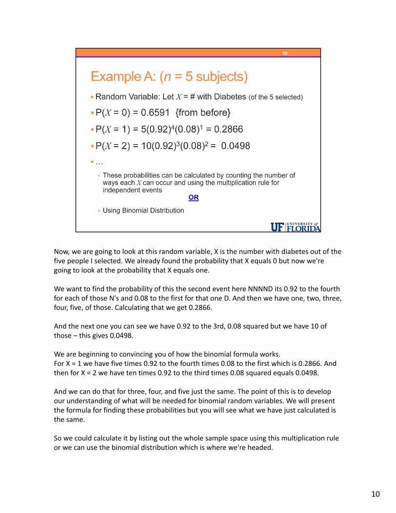
Now, we are going to look at this random variable, X is the number with diabetes out of the five people I selected. We already found the probability that X equals 0 but now we're going to look at the probability that X equals one. 

We want to find the probability of this the second event here NNNND its 0.92 to the fourth for each of those N's and 0.08 to the first for that one D. And then we have one, two, three, four, five, of those. Calculating that we get 0.2866. 

And the next one you can see we have 0.92 to the 3rd, 0.08 squared but we have 10 of those – this gives 0.0498. 

We are beginning to convincing you of how the binomial formula works. For X = 1 we have five times 0.92 to the fourth times 0.08 to the first which is 0.2866. And then for X = 2 we have ten times 0.92 to the third times 0.08 squared equals 0.0498. 

And we can do that for three, four, and five just the same. The point of this is to develop our understanding of what will be needed for binomial random variables. We will present the formula for finding these probabilities but you will see what we have just calculated is the same. 

So we could calculate it by listing out the whole sample space using this multiplication rule or we can use the binomial distribution which is where we're headed. 

10

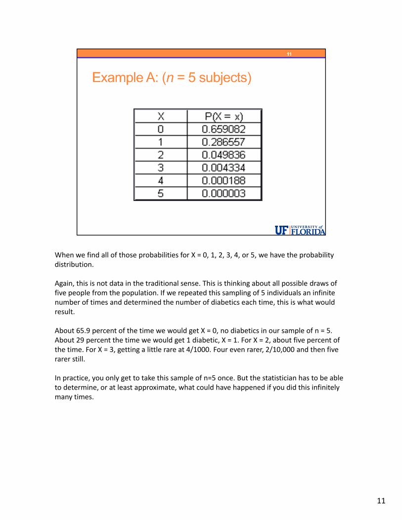
When we find all of those probabilities for X = 0, 1, 2, 3, 4, or 5, we have the probability distribution. 

Again, this is not data in the traditional sense. This is thinking about all possible draws of five people from the population. If we repeated this sampling of 5 individuals an infinite number of times and determined the number of diabetics each time, this is what would result. 

About 65.9 percent of the time we would get X = 0, no diabetics in our sample of n = 5. About 29 percent the time we would get 1 diabetic, X = 1. For X = 2, about five percent of the time. For X = 3, getting a little rare at 4/1000. Four even rarer, 2/10,000 and then five rarer still. 

In practice, you only get to take this sample of n=5 once. But the statistician has to be able to determine, or at least approximate, what could have happened if you did this infinitely many times. 

11

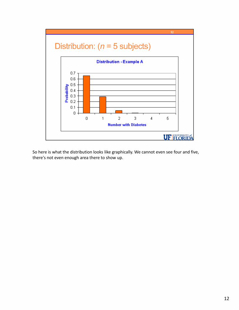
So here is what the distribution looks like graphically. We cannot even see four and five, there's not even enough area there to show up. 

12

Now we want to summarize this distribution by finding the mean and standard deviation. 

We found the mean or expected value using logic earlier and we will see that the formula we used applies to all binomial random variables but not necessarily all discrete random variables. We said that we would expect 8% of 5 to be diabetic which was 0.4. You can see how that is telling us that the center is closer to zero than one, more zeroes than ones. But 0 and 1 are most common. Two is pretty rare and three, four, and five, very rare. 

In general, for discrete random variables we have the following notation and equations. 

We have two notations for the mean here, one of them is MU, which is statistics notation for the population mean and the other is E(X) which is read as the expected value of X. 

Then we have the formula to calculate the mean for general discrete random variables. We take each value x_i, times the probability of that value, P(X = x_i) and then add those up. 

The variance can also be calculated – the notation which is most important is the greekSIGMA squared. We will see this notation used throughout the remainder of the course to represent the theoretical variance. The standard deviation is the square root of the variance, SIGMA. I won’t ask to calculate the variance on quizzes but it is illustrated here for both Example A and B if you are interested and also on the worksheet for this material. 

To review the notation, when we have a theoretical mean of a population or a theoretical distribution, we use MU or E(X). When we have a theoretical standard deviation it is lower case SIGMA and if I have a theoretical variance it is SIGMA squared. 

13

In Example A, we find the mean by taking each X value times the probability for that X value and add the results. Here there is a little rounding error since the exact value should be 0.4 and we found 0.399969. 

The variance is illustrated using the short‐cut formula where we square each x_i and then multiply by the probability for that X and add these results. Then we subtract the square of the mean. We have a variance of about 0.368. And taking the square root we get the standard deviation of 0.6065. 

We could also find other quantities such as the median, quartiles, percentiles, most anything that we found for quantitative variables is possible here but we will only discuss the mean and standard deviation and the overall idea of probability distributions for discrete random variables. 

14

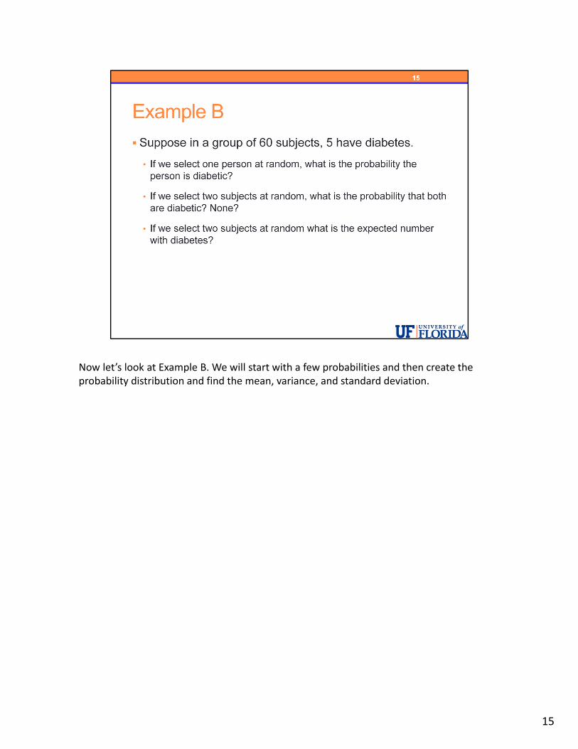
Now let’s look at Example B. We will start with a few probabilities and then create the probability distribution and find the mean, variance, and standard deviation. 

15

If we select one person at random from these 60 subjects where 5 were diabetic, what is the probability that the person is diabetic? If we pick one person we already said that it was 5 out of 60. Easy enough. 

16

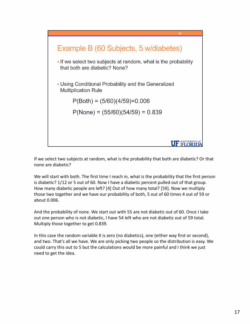
If we select two subjects at random, what is the probability that both are diabetic? Or that none are diabetic? 

We will start with both. The first time I reach in, what is the probability that the first person is diabetic? 1/12 or 5 out of 60. Now I have a diabetic percent pulled out of that group. How many diabetic people are left? [4] Out of how many total? [59]. Now we multiply those two together and we have our probability of both, 5 out of 60 times 4 out of 59 or about 0.006. 

And the probability of none. We start out with 55 are not diabetic out of 60. Once I take out one person who is not diabetic, I have 54 left who are not diabetic out of 59 total. Multiply those together to get 0.839. 

In this case the random variable X is zero (no diabetics), one (either way first or second), and two. That's all we have. We are only picking two people so the distribution is easy. We could carry this out to 5 but the calculations would be more painful and I think we just need to get the idea. 

17

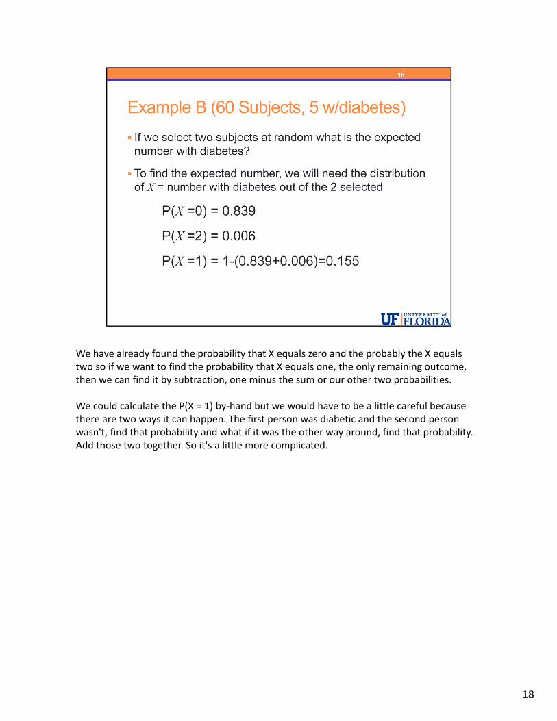
We have already found the probability that X equals zero and the probably the X equals two so if we want to find the probability that X equals one, the only remaining outcome, then we can find it by subtraction, one minus the sum or our other two probabilities. 

We could calculate the P(X = 1) by‐hand but we would have to be a little careful because there are two ways it can happen. The first person was diabetic and the second person wasn't, find that probability and what if it was the other way around, find that probability. Add those two together. So it's a little more complicated. 

18

Here is the probability distribution in Example B. 

To find the mean, we take each value times the probability of that value and then add the results to get 0.167. 

This is similar to a weighted average, like your GPA. If we want to calculate things based upon probability distributions we have to take into account how likely each value would be. 

19

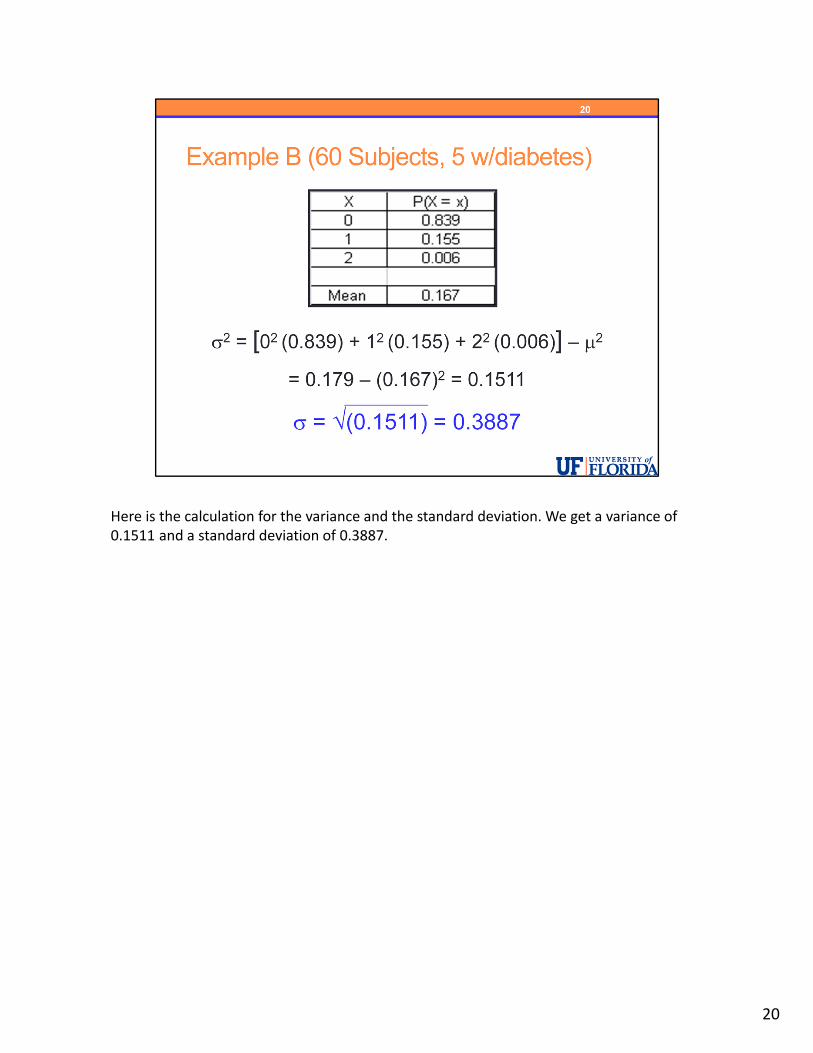
Here is the calculation for the variance and the standard deviation. We get a variance of 0.1511 and a standard deviation of 0.3887. 

20

Working with probability distributions is an important application of probability to statistics. You will need to be able to find probabilities about a discrete random variable from a given probability distribution and to find the mean of the random variable. You should understand the notation for the variance and standard deviation but will not need to calculate these yourself on assessments in the course. 

Next we will learn more about a specific type of discrete random variable called the binomial. 

21