November 2005CSA3180: Statistics II1 CSA3180: Natural Language Processing Statistics 2 – Probability and Classification II Experiments/Outcomes/Events

November 2005 CSA3180: Statistics II 1

CSA3180: Natural Language Processing

Statistics 2 – Probability and Classification II

• Experiments/Outcomes/Events• Independence/Dependence• Bayes’ Rule• Conditional Probabilities/Chain Rule• Classification II


Introduction

• Slides based on Lectures by Mike Rosner (2003) and material by Mary Dalrymple, Kings College, London


Experiments, Basic Outcome, Sample Space

• Probability theory is founded upon the notion of an experiment.

• An experiment is a situation which can have one or more different basic outcomes.

• Example: if we throw a die, there are six possible basic outcomes.

• A Sample Space Ω is a set of all possible basic outcomes. For example,– If we toss a coin, Ω = {H,T}– If we toss a coin twice, Ω = {HT,TH,TT,HH}– if we throw a die, Ω = {1,2,3,4,5,6}


Events

• An Event A Ω is a set of basic outcomes e.g.– tossing two heads {HH}– throwing a 6, {6}– getting either a 2 or a 4, {2,4}.

• Ω itself is the certain event, whilst { } is the impossible event.

• Event Space ≠ Sample Space


Probability Distribution

• A probability distribution of an experiment is a function that assigns a number (or probability) between 0 and 1 to each basic outcome such that the sum of all the probabilities = 1.

• Probability distribution functions (PDFs)

• The probability p(E) of an event E is the sum of the probabilities of all the basic outcomes in E.

• Uniform distribution is when each basic outcome is equally likely.


Probability of an Event

• Sample space for a die throw = set of basic outcomes = {1,2,3,4,5,6}

• If the die is not loaded, distribution is uniform.

• Thus for each basic outcome, e.g. {6} (throwing a six) is assigned the same probability = 1/6.

• So p({3,6}) = p({3}) + p({6}) = 2/6 = 1/3


Probability Estimates

• Repeat experiment T times and count frequency of E.

• Estimated p(E) = count(E)/count(T)

• This can be done over m runs, yielding estimates p1(E),...pm(E).

• Best estimate is (possibly weighted) average of individual pi(E)


3 Times Coin Toss

• Ω = {HHH,HHT,HTH,HTT,THH,THT,TTH,TTT}• Cases with exactly 2 tails = {HTT, THT,TTH}

• Experimenti = 1000 cases (3000 tosses).

– c1(E)= 386, p1(E) = .386

– c2(E)= 375, p2(E) = .375

– pmean(E)= (.386+.375)/2 = .381

• Uniform distribution is when each basic outcome is equally likely.

• Assuming uniform distribution, p(E) = 3/8 = .375


Word Probability

• General Problem:What is the probability of the next word/character/phoneme in a sequence, given the first N words/characters/phonemes.

• To approach this problem we study an experiment whose sample space is the set of possible words.

• Same approach could be used to study the the probability of the next character or phoneme.


Word Probability

• I would like to make a phone _____.

• Look it up in the phone ________, quick!

• The phone ________ you requested is…

• Context can have decisive effect on word probability


Word Probability

• Approximation 1: all words are equally probable

• Then probability of each word = 1/N where N is the number of word types.

• But all words are not equally probable

• Approximation 2: probability of each word is the same as its frequency of occurrence in a corpus.


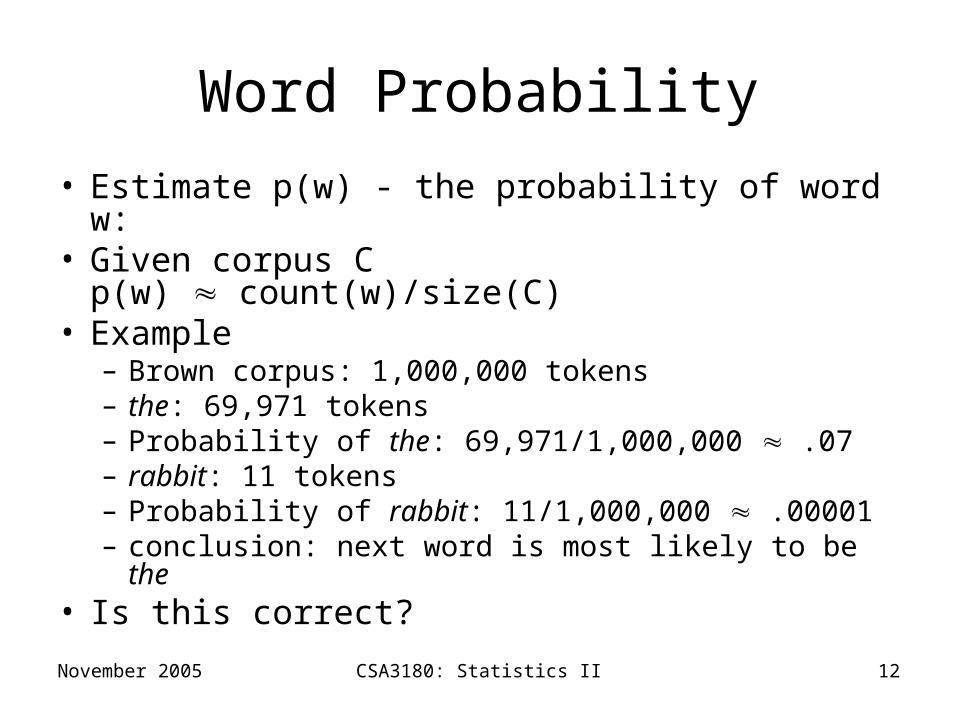
Word Probability

• Estimate p(w) - the probability of word w:• Given corpus C

p(w) count(w)/size(C) • Example

– Brown corpus: 1,000,000 tokens– the: 69,971 tokens– Probability of the: 69,971/1,000,000 .07– rabbit: 11 tokens– Probability of rabbit: 11/1,000,000 .00001– conclusion: next word is most likely to be the

• Is this correct?


Word Probability

• Given the context: Look at the cute ...

• is the more likely than rabbit?

• Context matters in determining what word comes next.

• What is the probability of the next word in a sequence, given the first N words?


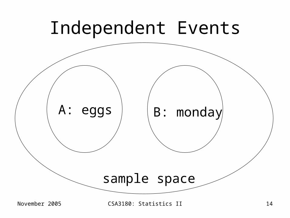
Independent Events

A: eggs B: monday

sample space


Sample Space

(eggs,mon) (cereal,mon) (nothing,mon)

(eggs,tue) (cereal,tue) (nothing,tue)

(eggs,wed) (cereal,wed) (nothing,wed)

(eggs,thu) (cereal,thu) (nothing,thu)

(eggs,fri) (cereal,fri) (nothing,fri)

(eggs,sat) (cereal,sat) (nothing,sat)

(eggs,sun) (cereal,sun) (nothing,sun)


Independent Events

• Two events, A and B, are independent if the fact that A occurs does not affect the probability of B occurring.

• When two events, A and B, are independent, the probability of both occurring p(A,B) is the product of the prior probabilities of each, i.e.

p(A,B) = p(A) · p(B)


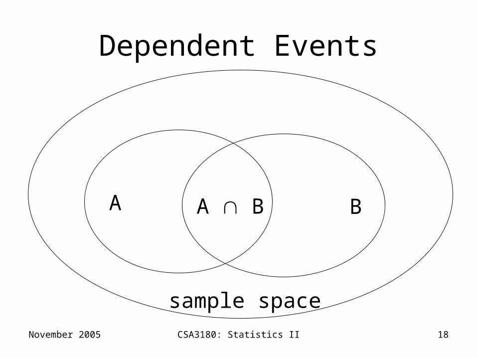
Dependent Events

• Two events, A and B, are dependent if the occurrence of one affects the probability of the occurrence of the other.


Dependent Events

A B

sample space

A B


Conditional Probability

• The conditional probability of an event A given that event B has already occurred is written p(A|B)

• In general p(A|B) p(B|A)


Dependent Events: p(A|B)≠ p(B|A)

A

B

sample space

A B


Example Dependencies

• Consider fair die example with– A = outcome divisible by 2– B = outcome divisible by 3– C = outcome divisible by 4

• p(A|B) = p(A B)/p(B) = (1/6)/(1/3) = ½

• p(A|C) = p(A C)/p(C) = (1/6)/(1/6) = 1


Conditional Probability

• Intuitively, after B has occurred, event A is replaced by A B, the sample space Ω is replaced by B, and probabilities are renormalised accordingly

• The conditional probability of an event A given that B has occurred (p(B)>0) is thus given by p(A|B) = p(A B)/p(B).

• If A and B are independent,p(A B) = p(A) · p(B) sop(A|B) = p(A) · p(B) /p(B) = p(A)


Bayesian Inversion

• For A and B to occur, either B must occur first, then B, or vice versa. We get the following possibilites:p(A|B) = p(A B)/p(B)p(B|A) = p(A B)/p(A)

• Hence p(A|B) p(B) = p(B|A) p(A)• We can thus express p(A|B) in terms of p(B|A)• p(A|B) = p(B|A) p(A)/p(B)• This equivalence, known as Bayes’ Theorem, is

useful when one or other quantity is difficult to determine


Bayes’ Theorem

• p(B|A) = p(BA)/p(A) = p(A|B) p(B)/p(A)

• The denominator p(A) can be ignored if we are only interested in which event out of some set is most likely.

• Typically we are interested in the value of B that maximises an observation A, i.e.

• arg maxB p(A|B) p(B)/p(A) = arg maxB p(A|B) p(B)


Chain Rule

• We can use the definition of conditional probability to more than two events

• p(A1 ... An) = p(A1) * p(A2|A1) * p(A3|A1 A2)..., p(An|A1 ... An-1)

• The chain rule allows us to talk about the probability of sequences of events p(A1,...,An)


Classification II

• Linear algorithms in Classification I

• Non-linear algorithms

• Kernel methods

• Multi-class classification

• Decision trees

• Naïve Bayes


Non-Linear Problems


Non-Linear Problems


Non-Linear Problems

• Kernel methods

• A family of non-linear algorithms

• Transform the non linear problem in a linear one (in a different feature space)

• Use linear algorithms to solve the linear problem in the new space


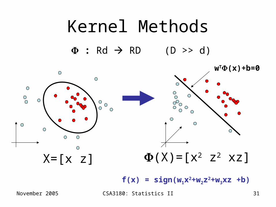
Kernel Methods

• Linear separability: more likely in high dimensions

• Mapping: maps input into high-dimensional feature space

• Classifier: construct linear classifier in high-dimensional feature space

• Motivation: appropriate choice of leads to linear separability

• We can do this efficiently!


Kernel Methods

X=[x z]

: Rd RD (D >> d)

(X)=[x2 z2 xz]

f(x) = sign(w1x2+w2z2+w3xz +b)

wT(x)+b=0


Kernel Methods

• We can use the linear algorithms seen before (Perceptron, SVM) for classification in the higher dimensional space

• Kernel methods basically transform any algorithm that solely depend on dot product between two vectors by replacing dot with kernel function

• Non-linear kernel algorithm is the linear algorithm operating in the range space of

• The is never explicitly computed (kernels are used instead)


Multi-class Classification

• Given: some data items that belong to one of M possible classes

• Task: Train the classifier and predict the class for a new data item

• Geometrically: harder problem, no more simple geometry





• Author identification

• Language identification

• Text categorization (topics)



• Linear– Parallel class separators: Decision Trees– Non parallel class separators: Naïve

Bayes

• Non Linear– K-nearest neighbors


Linear, parallel class separators (e.g. Decision Trees)


Linear, non-parallel class separators (e.g. Naïve Bayes)


Non-Linear separators (e.g. k Nearest Neighbors)


Decision Trees

• Decision tree is a classifier in the form of a tree structure, where each node is either:– Leaf node - indicates the value of the target

attribute (class) of examples, or– Decision node - specifies some test to be

carried out on a single attribute-value, with one branch and sub-tree for each possible outcome of the test.

• A decision tree can be used to classify an example by starting at the root of the tree and moving through it until a leaf node, which provides the classification of the instance.


NoStrongHighMildRainD14YesWeakNormalHotOvercastD13YesStrongHighMildOvercastD12YesStrongNormalMildSunnyD11YesStrongNormalMildRainD10YesWeakNormalColdSunnyD9NoWeakHighMildSunnyD8YesWeakNormalCoolOvercastD7NoStrongNormalCoolRainD6YesWeakNormalCoolRainD5YesWeakHighMildRain D4 YesWeakHighHotOvercastD3NoStrongHighHotSunnyD2NoWeakHighHotSunnyD1

Play TennisWindHumidityTemp.OutlookDay

Goal: learn when we can play Tennis and when we cannot


Decision TreesOutlook

Sunny Overcast Rain

Humidity

High Normal

Wind

Strong Weak

No Yes

Yes

YesNo


Decision TreesOutlook

Sunny Overcast Rain

Humidity

High Normal

No Yes

Each internal node tests an attribute

Each branch corresponds to anattribute value node

Each leaf node assigns a classification


No

Outlook

Sunny Overcast Rain

Humidity

High Normal

Wind

Strong Weak

No Yes

Yes

YesNo

Outlook Temperature Humidity Wind PlayTennis Sunny Hot High Weak ?


Decision Tree for Reuters


Decision Trees for Reuters


Building Decision Trees

• Given training data, how do we construct them?• The central focus of the decision tree growing

algorithm is selecting which attribute to test at each node in the tree. The goal is to select the attribute that is most useful for classifying examples.

• Top-down, greedy search through the space of possible decision trees.– That is, it picks the best attribute and never

looks back to reconsider earlier choices.


Building Decision Trees• Splitting criterion

– Finding the features and the values to split on • for example, why test first “cts” and not “vs”? • Why test on “cts < 2” and not “cts < 5” ?

– Split that gives us the maximum information gain (or the maximum reduction of uncertainty)

• Stopping criterion– When all the elements at one node have the same class, no need to

split further• In practice, one first builds a large tree and then one prunes it back

(to avoid overfitting)

• See Foundations of Statistical Natural Language Processing, Manning and Schuetze for a good introduction

http://nlp.stanford.edu/fsnlp/


Decision Trees: Strengths

• Decision trees are able to generate understandable rules.

• Decision trees perform classification without requiring much computation.

• Decision trees are able to handle both continuous and categorical variables.

• Decision trees provide a clear indication of which features are most important for prediction or classification.


Decision Trees: Weaknesses

• Decision trees are prone to errors in classification problems with many classes and relatively small number of training examples.

• Decision tree can be computationally expensive to train. – Need to compare all possible splits– Pruning is also expensive

• Most decision-tree algorithms only examine a single field at a time. This leads to rectangular classification boxes that may not correspond well with the actual distribution of records in the decision space.


Naïve BayesMore powerful that Decision Trees

Decision Trees Naïve Bayes


Naïve Bayes

• Graphical Models: graph theory plus probability theory

• Nodes are variables• Edges are

conditional probabilities

A

B C

P(A) P(B|A)P(C|A)


Naïve Bayes• Graphical Models: graph

theory plus probability theory

• Nodes are variables• Edges are conditional

probabilities• Absence of an edge

between nodes implies independence between the variables of the nodes

A

B C

P(A) P(B|A)P(C|A) P(C|A,B)


Naïve Bayes


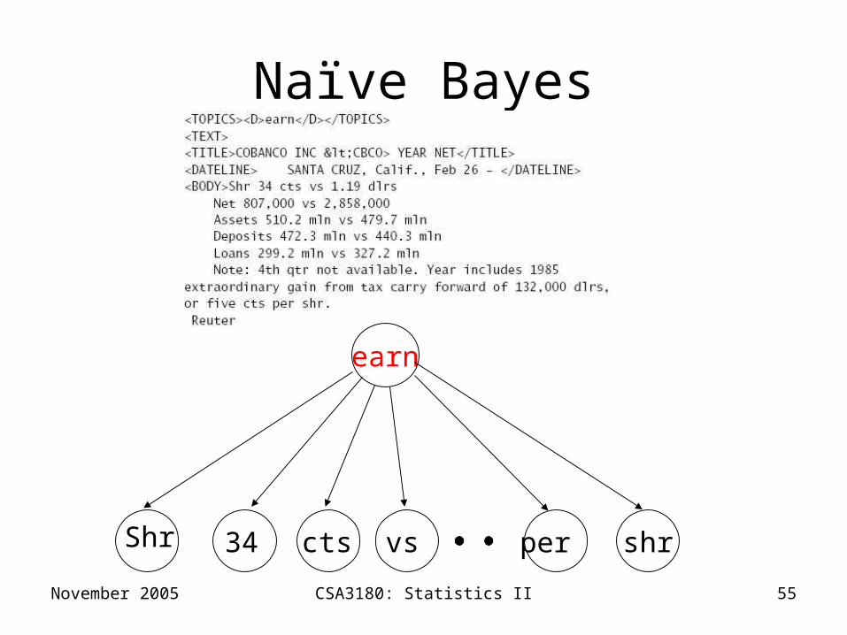
Naïve Bayes

earn

Shr 34 cts vs shrper


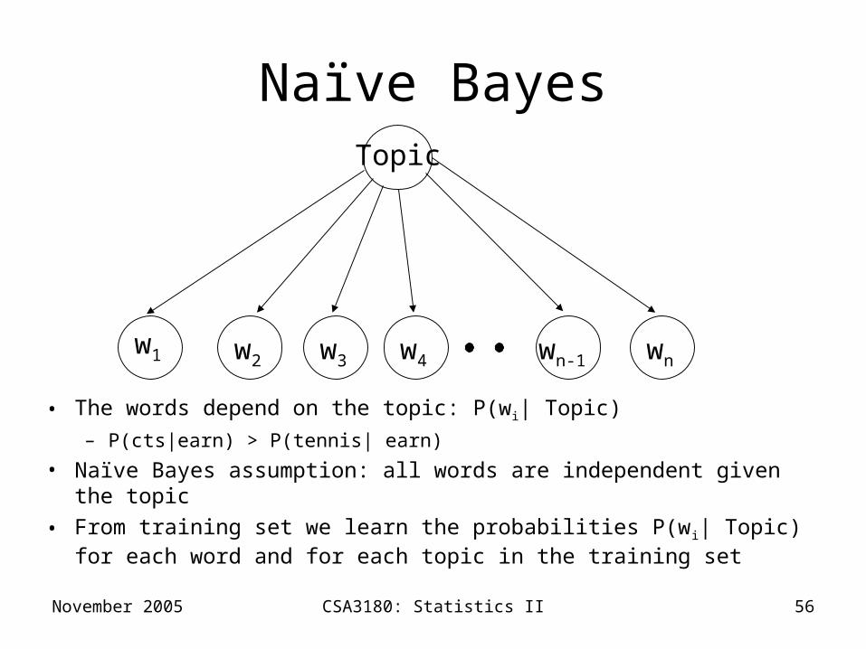
Naïve Bayes

• The words depend on the topic: P(wi| Topic)

– P(cts|earn) > P(tennis| earn)

• Naïve Bayes assumption: all words are independent given the topic

• From training set we learn the probabilities P(wi| Topic) for each word and for each topic in the training set

Topic

w1 w2 w3 w4 wnwn-1


Naïve Bayes

• To: Classify new example

• Calculate P(Topic | w1, w2, … wn) for each topic

• Bayes decision rule:– Choose the topic T’ for which

– P(T’ | w1, w2, … wn) > P(T | w1, w2, … wn) for each T T’

Topic

w1 w2 w3 w4 wnwn-1


Naïve Bayes: Math

• Naïve Bayes define a joint probability distribution:

• P(Topic , w1, w2, … wn) = P(Topic) P(wi| Topic)

• We learn P(Topic) and P(wi| Topic) in training

• Test: we need P(Topic | w1, w2, … wn)

• P(Topic | w1, w2, … wn) = P(Topic , w1, w2, … wn) / P(w1, w2, … wn)


Naïve Bayes: Strengths

• Very simple model– Easy to understand– Very easy to implement

• Very efficient, fast training and classification• Modest space storage• Widely used because it works really well for text

categorization• Linear, but non parallel decision boundaries


Naïve Bayes: Weaknesses

• Naïve Bayes independence assumption has two consequences:– The linear ordering of words is ignored (bag of words

model)– The words are independent of each other given the

class: False • President is more likely to occur in a context that contains

election than in a context that contains poet

• Naïve Bayes assumption is inappropriate if there are strong conditional dependencies between the variables

• (But even if the model is not “right”, Naïve Bayes models do well in a surprisingly large number of cases because often we are interested in classification accuracy and not in accurate probability estimations)

Documents

November 2005CSA3180: Statistics II1 CSA3180: Natural Language Processing Statistics 2 – Probability and Classification II Experiments/Outcomes/Events