Embed Size (px)
Citation preview

NOVEL TURBO EQUALIZATION METHODS FOR THE MAGNETIC
RECORDING CHANNEL
A Dissertation Presented to
The Academic Faculty
By
Elizabeth Chesnutt
In Partial Fulfillment Of the Requirements for the Degree of
Doctor of Philosophy in Electrical and Computer Engineering
Georgia Institute of Technology
May 2005
Copyright © Elizabeth Chesnutt 2005

NOVEL TURBO EQUALIZATION METHODS FOR THE MAGNETIC
RECORDING CHANNEL
Approved by:
Dr. John Barry, Advisor
School of Electrical and Computer Engineering Georgia Institute of Technology Dr. Ye (Geoffrey) Li School of Electrical and Computer Engineering Georgia Institute of Technology Dr. Steve McLaughlin School of Electrical and Computer Engineering Georgia Institute of Technology Date Approved: April 11, 2005
ii

This work is dedicated to my husband Leandro
whose strength, support, and love
I will always cherish.

ACKNOWLEDGEMENT Completing a Ph.D. is truly a marathon event, and I would not have been able to
conclude this endeavor without the aid and encouragement of countless people over the
past few years. I must first express my gratitude towards my advisor, Professor John R.
Barry. His leadership, support, attention to detail, and hard work has set an example I
hope to match some day.
I would like to thank the many graduate students I have worked with in the
Communication Theory Group for their insights and invaluable comments over the years:
Renato Lopes, Pornchai (Mai) Supnithi, Estaurdo Licona-Nuñez, Andrew Thangaraj,
Badri Varadarajan, Aravind Nayak, Piya Kovintavewat, and Deric Waters. I look
forward to a continuing collaboration with them in the future.
I also thank some of my other fellow Ph.D. students: Apurva Mody, Brian Delaney,
Cagatay Candan, Loren Jatunov, and Babak Firoozbakhsh. They each helped make my
time in the Ph.D. program more fun and interesting. I especially thank Apurva for his
willingness to listen, his enthusiasm for life, and his continuous dreams in the best of this
world.
This research has definitely profited from the friendship, advice, and encouragement
of several remarkable people: Jessica & Alex Turner, Allison Harrelson, Miles Edson,
Jeanette Anderson, Rick Hargett, Wendy Anderson, Natalia Landazuri, Mario Romero,
iv

and Heather Brandt. They have stimulated much of my happiness and entertainment, and
I feel privileged that these people have accepted me as a friend. I am also extremely
appreciative of the care and assistance given to me by Roxie Baxter during an especially
trying time.
My family has been superb source of support. Even with our usual sibling fighting
when we were younger, my brother Jason is a wonderfully considerate person and his
friendship has been a blessing. I could not have handpicked a better brother. I am also
grateful for the encouragement and love of my cousins Jeremy, Josh, and Jennifer
Adams, who have always been like siblings to me.
Special thanks are due to my husband, Leandro Barajas, who has been an advisor,
consultant, friend, and my biggest advocate in this long journey. Without his love and
understanding, this arduous task would have been vastly more difficult. Estoy por
siempre en deuda contigo por tu amor y ayuda.
Lastly, I would like to give a shout out to Scott Woods to whom in third grade
I emphatically declared that I would one day write a book. Well here it is, but not quite
what I had envisioned as a third grader. But is it not wonderful how our lives have
unfolded out in front of us?
This research and this dissertation are results of collaboration and support. Thank
you God and all of you who have assisted me in this exciting journey.
v

TABLE OF CONTENTS
ACKNOWLEDGMENT iv
LIST OF TABLES x
LIST OF FIGURES xi
LIST OF EQUATIONS xiv
LIST OF SYMBOLS OR ABBREVIATIONS xv
SUMMARY xxi
CHAPTER 1. INTRODUCTION 1
1.1 The Problem.................................................................................................... 1
1.2 Objective ......................................................................................................... 3
1.3 Outline............................................................................................................. 4
CHAPTER 2. ORIGIN AND HISTORY OF THE PROBLEM 5
2.1 Digital Magnetic Recording............................................................................ 5
vi

2.2 Channel Characteristics .................................................................................. 7
2.3 Optimum Detector ........................................................................................ 12
2.4 Partial Response............................................................................................ 13
2.5 Channel Detection with PR Equalization ..................................................... 15
2.5.1 Complexity Considerations................................................................... 16
2.5.2 The BCJR Algorithm ............................................................................ 18
2.5.3 State-of-the-Art Channel Detection in Magnetic Recording ................ 21
2.6 Turbo Equalization........................................................................................ 22
2.6.1 The APP Module................................................................................... 23
2.6.2 Iterative Equalization with APP Modules............................................. 24
2.6.3 Turbo Equalization for the MRC .......................................................... 27
CHAPTER 3. THE NOISE-PREDICTIVE BCJR ALGORITHM 29
3.1 Introduction................................................................................................... 29
3.2 Noise Correlation .......................................................................................... 30
3.3 Conventional BCJR with colored noise........................................................ 33
3.3.1 Noise Memory in Branch Transition Probabilities ............................... 33
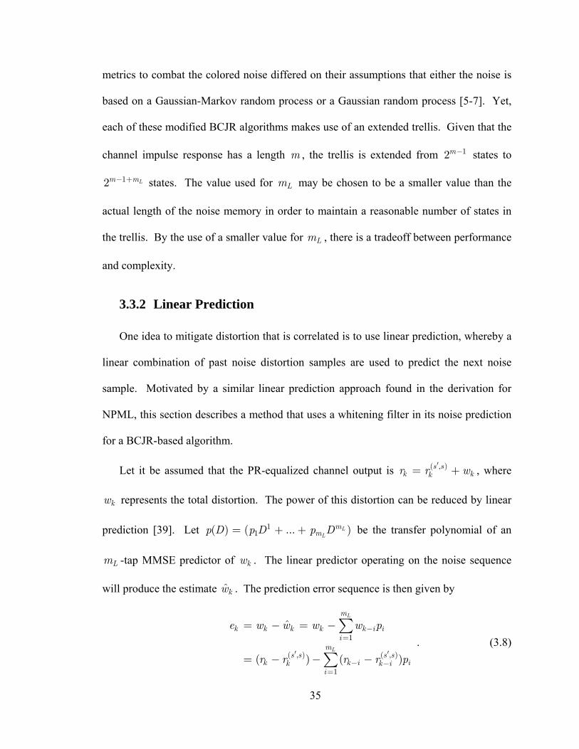
3.3.2 Linear Prediction................................................................................... 35
3.4 Noise-Predictive BCJR ................................................................................. 37
3.5 Results........................................................................................................... 42
CHAPTER 4. BEYOND PRML: LINEAR-COMPLEXITY TURBO EQUALIZATION USING THE SOFT-FEEDBACK EQUALIZER 47
vii

4.1 Introduction................................................................................................... 47
4.2 The SFE Algorithm Alternative to Partial-Response Equalization .............. 49
4.2.1 The SFE Algorithm............................................................................... 50
4.2.2 The SFE Algorithm and Turbo Equalization ........................................ 53
4.2.3 Alternative Equalizer Structure for the MRC ....................................... 56
4.3 Simulations ................................................................................................... 57
4.3.1 System Model Comparisons ................................................................. 57
4.3.2 Turbo Code Results............................................................................... 58
4.3.3 LDPC Results........................................................................................ 60
4.3.4 Comparison with NPML....................................................................... 64
4.3.5 Results................................................................................................... 64
CHAPTER 5. NOVEL SFE CALCULATIONS FOR THE MRC 66
5.1 Introduction................................................................................................... 66
5.2 The computation of and .................................................................. 67 eγ pγ
5.3 The Matrix Inverse........................................................................................ 72
5.3.1 Conjugate Gradient Method.................................................................. 73
5.3.2 Incomplete Basis Method ..................................................................... 76
5.4 Results........................................................................................................... 83
CHAPTER 6. CONCLUSIONS 86
6.1 Summary of the Contributions...................................................................... 86
viii

6.2 Proposed Future Work .................................................................................. 88
REFERENCES 90
VITA 95
ix

LIST OF TABLES
Table 5.1: Comparison results of the CG-method filter to the original SFE filter ...........76
Table 5.2: Comparison results of the incomplete basis method to the original SFE filter ............................................................................................................................81
x

LIST OF FIGURES
Figure 2.1. Physical components of a magnetic recording system......................................6
Figure 2.2. Magnetized particles in the media.....................................................................6
Figure 2.3. Transition response............................................................................................8
Figure 2.4. Overall impulse response ..................................................................................9
Figure 2.5. Normalized versions of for different values of ............................10 ( cS fT )
) )
cD
Figure 2.6. Magnetic recording channel ............................................................................11
Figure 2.7. Discrete-time magnetic recording channel......................................................11
Figure 2.8. Optimal detector ..............................................................................................12
Figure 2.9. Normalized frequency response of and ..................15 4(PR cH fT 4(EPR cH fT
Figure 2.10. Example of trellis diagram for a 4-state finite-state machine........................17
Figure 2.11. System diagram with encoder, MRC, PR equalizer, BCJR channel detector, and decoder..................................................................................................................22
Figure 2.12. APP module...................................................................................................24
Figure 2.13. The turbo equalization process as an iterative loop.......................................25
Figure 2.14. System diagram with encoder, MRC, PR equalizer, BCJR channel detector, and decoder employing turbo equalization..................................................................27
Figure 3.1. The MRC with the discrete-time model, the matched filter, and the PR
equalizer.......................................................................................................................31 Figure 3.2. The frequency response of the PR equalizers for the ZF and MMSE
formulations with , , and using the PR4 target...........................32 2.0cD = 0 0.8N =
xi

Figure 3.3. The PSD of the total distortion for the ZF and MMSE formulations with , , and using the PR4 target ........................................................33 2.0cD = 0 0.8N =
Figure 3.4. Hypothetical survivor path memories in a section of the trellis using the
NP-BCJR with a PR4 target ........................................................................................40 Figure 3.5. Hypothetical state transitions in a section of the trellis using the NP-BCJR
with a PR4 target .........................................................................................................41 Figure 3.6. System model with turbo equalization over the magnetic recording channel.43
Figure 3.7. BER performance of the classic BCJR, extended trellis BCJR, and the NP-BCJR for channel density 2.0, PR4.......................................................................44
Figure 3.8. Complexity comparison of the classic BCJR, extended trellis BCJR, and the
NP-BCJR for channel density 2.0, PR4, BER=10-5 ....................................................45 Figure 3.9. BER performance comparison of the classic BCJR, extended trellis BCJR,
and the NP-BCJR for channel density 2.5, EPR4........................................................46 Figure 3.10. Complexity comparison of the classic BCJR, extended trellis BCJR, and the
NP-BCJR for channel density 2.5, EPR4, BER=10-5 ..................................................46 Figure 4.1. Interference canceller with a priori information..............................................51
Figure 4.2. SFE equalizer structure....................................................................................52
Figure 4.3. Turbo equalizer using an SFE channel detector ..............................................54
Figure 4.4. The turbo equalization SFE structure for the magnetic recording channel .....56
Figure 4.5. BER performance comparison of the PR system and the SFE system with a rate-8/9 (23,31) turbo code, ........................................................................59 3.0cD =
Figure 4.6. Comparison of PR system and SFE system with a rate-8/9 (23,31) turbo code
with fixed BER=10-5 over a range of ....................................................................60 cD Figure 4.7. BER and SER comparisons of the PR system and SFE system with a rate-8/9
(4095,3640) regular LDPC code, ...............................................................61 2.0cD = Figure 4.8. Comparison of the PR system and SFE system with a rate-8/9 (4095,3640)
regular LDPC code with fixed BER=10-5 over a range of ....................................62 cD Figure 4.9. Complexity-performance comparison of the SFE system and the PR4-
equalized system with a rate-8/9 (4095,3640) regular LDPC code with fixed BER=10-5 at channel density 2.5 .................................................................................63
xii

Figure 4.10. BER performance comparison for data with RS (255, 239, 17) code at channel density 2.0 ......................................................................................................65
Figure 5.1. Scatter plots of versus for turbo iterations 2 through 5, ,
SNR = 8.5 dB...............................................................................................................70 eγ 2.0cD =pγ
Figure 5.2. Average across sectors for each turbo iteration for varying channel
densities at an SNR that gives BER=10-5 at the fifth turbo iteration...........................72 ,e iγ
Figure 5.3. 3-D plot of all possible feed-forward filters at the given channel setup with
channel density 2.5 and SNR = 11.5 dB......................................................................81 Figure 5.4. Basis coefficient values as changes for channel density 2.5 and
SNR = 11.5 dB.............................................................................................................82 pγ
Figure 5.5. BER and SER performance curves for the original SFE and the SFE with
basis functions at ........................................................................................84 2.0cD = Figure 5.6. Overhead complexity versus performance of the original SFE and the SFE
with basis functions at .................................................................................85 2.0cD =
xiii

LIST OF EQUATIONS Eq. (2.1) ...................7 Eq. (2.19) ...............21 Eq. (4.3) .................52
Eq. (2.2) ...................7 Eq. (3.1) .................30 Eq. (4.4) .................52
Eq. (2.3) ...................9 Eq. (3.2) .................31 Eq. (4.5) .................53
Eq. (2.4) ...................9 Eq. (3.3) .................31 Eq. (4.6) .................53
Eq. (2.5) .................10 Eq. (3.4) .................31 Eq. (4.7) .................53
Eq. (2.6) .................11 Eq. (3.5) .................32 Eq. (4.8) .................53
Eq. (2.7) .................14 Eq. (3.6) .................34 Eq. (5.1) .................71
Eq. (2.8) .................14 Eq. (3.7) .................34 Eq. (5.2) .................73
Eq. (2.9) .................19 Eq. (3.8) .................35 Eq. (5.3) .................74
Eq. (2.10) ...............19 Eq. (3.9) .................36 Eq. (5.4) .................76
Eq. (2.11) ...............19 Eq. (3.10) ...............36 Eq. (5.5) .................77
Eq. (2.12) ...............19 Eq. (3.11) ...............36 Eq. (5.6) .................77
Eq. (2.13) ...............19 Eq. (3.12) ...............36 Eq. (5.7) .................79
Eq. (2.14) ...............20 Eq. (3.13) ...............37 Eq. (5.8) .................79
Eq. (2.15) ...............20 Eq. (3.14) ...............38 Eq. (5.9) .................79
Eq. (2.16) ...............20 Eq. (3.15) ...............39 Eq. (5.10) ...............79
Eq. (2.17) ...............20 Eq. (4.1) .................51 Eq. (5.11) ...............79
Eq. (2.18) ...............20 Eq. (4.2) .................52 Eq. (5.12) ...............82
xiv

LIST OF SYMBOLS OR ABBREVIATIONS APP A Posteriori Probability
AWGN Additive White Gaussian Noise
BCJR Bahl-Cocke-Jelinek-Raviv
BER Bit Error Rate
BPSK Binary Phase Shift Keying
CG Conjugate Gradient
DFE Decision-Feedback Equalizer
ECC Error Correction Coding
IC Interference Cancellation
ISI Intersymbol Interference
FSM Finite-State Machine
FT Fourier Transform
LE Linear Equalizer
LDPC Low-Density Parity-Check
LLR Log Likelihood Ratio
LTI Linear Time-Invariant
NPML Noise-Predictive Maximum-Likelihood
MAC Multiply-Accumulate
xv

MAP Maximum A Posteriori
MDFE Multi-level Decision Feedback Equalizer MF Matched Filter MLSD Maximum Likelihood Sequence Detector
MMSE Minimum Mean-Square Error
MR Magneto-resistive
MRC Magnetic Recording Channel
NP-BCJR Noise Predictive BCJR
NRZ Non-Return to Zero
PR Partial Response
PRML Partial-Response Maximum-Likelihood
PSD Power Spectral Density
RAM Random-Access Memory
RS Reed-Solomon
SEM Simplified Expectation-Maximization
SER Sector Error Rate
SFE Soft-Decision Feedback Equalizer (with priors)
SISO Soft-Input Soft-Output
SNR Signal to Noise Ratio
SOVA Soft-Output Viterbi Algorithm
ZF Zero-Forcing
Encoded data symbols ka
Transition sequence in the magnetic media kc
xvi
( )c D PR equalizer
Delay operator D
Recorded bit density cD
User bit density uD
Energy in an isolated transition pulse iE
( )f D Discrete-time magnetic recording channel model
f Feed-forward filter of the SFE
ICf Traditional ISI canceller that the SFE feed-forward filter reduces to as pγ → ∞
f Subset of all possible vectors for a given channel setup F
SNR of the a priori information aγ
SNR of the extrinsic information eγ
Discrete-time transition pulse kg
( )PRg D Target response
1g Feedback filter of the SFE working with only a priori information
2g Feedback filter of the SFE working with the full LLR information
H Channel convolution matrix
LDPCH Parity check matrix for an LDPC code
Coercivity cH
( cH fT ) Frequency-normalized Fourier-transform of the transition response
( )h t Transition response
0th column of 0h H
xvii

Discrete-time channel kh
Discrete time index k
Extrinsic LLR calculated by the equalizer kλ
pkλ A priori LLR available to the equalizer
Sector length L
LLR of transmitted symbols kL
( , )M s s′ Partial path metric
PR-equalized channel length m
Length of distortion prediction filter Lm
Length of discrete channel μ
Length of SFE feed-forward filter N
1g Length of SFE feedback filter 1N
2g Along with , determines the length of the SFE feedback filter μ2N
The maximum number of inner iterations for the decoder per outer turbo iNequalization iteration
Power spectral density of the AWGN oN
Determines the order of the Thapar-Patel target polynomial n
Discrete-time additive noise kn
( )n t Additive noise in the MRC
Basis coefficient mν
Interleaver π
1π− Deinterleaver
Number of turbo equalization iterations P
xviii

Width of Lorentzian pulse at half its maximum 50PW
( )p D MMSE predictor filter of the total distortion
kp Search direction vector in the CG algorithm
( )q D Minimum phase causal factor of 1/ ( )wR D
kq Residuals in the CG algorithm
( )fR D -transform of the discrete-time channel autocorrelation coefficients D
( )wR D -transform of the autocorrelation of the total distortion D
Encoder rate r
( )r t Read-back signal
S+ Set of all ordered pairs ( , corresponding to all state transitions caused )s s′by the input 1ka = +
S− Set of all ordered pairs ( , corresponding to all state transitions caused )s s′ by the input 1ka = −
( )cS fT Frequency-normalized Fourier-transform of the overall impulse response
State of trellis-based encoder at time 1k −s
s′ State of trellis-based encoder at time k
( )s t Overall impulse response of the MRC
( )s t− Filter matched to the channel ( )s t
2σ Noise variance
2aσ Average symbol energy of the sequence ka
LDPCH Column weight of the matrix t
Recorded bit duration cT
xix

mφ Basis function
Output of prediction filter 1 ( kv )p D−
( )w D -transform of the total distortion seen by the detector D
Input symbols to the encoder kx
Output sequence of the partial response equalizer ky
xx

SUMMARY The topic of this dissertation is the derivation, development, and evaluation of novel
turbo equalization techniques that address the colored noise problem on the magnetic
recording channel. One new algorithm presented is the noise-predictive BCJR, which is
a soft-output detection strategy that mitigates colored noise in partial-response equalized
magnetic recording channels. This algorithm can be viewed as a combination of the
traditional BCJR algorithm with the notion of survivors and noise prediction.
Additionally, an alternative equalization architecture for magnetic recording is
presented that addresses the shortcomings of the PRML approach, which dominates
magnetic recording. Specifically, trellis-based equalizers are abandoned in favor of
simple equalization strategies based on nonlinear filters whose complexity grows only
linearly with their length. This research focuses on the linear-complexity SFE algorithm
and on investigating the possibility of lowering the SFE filter calculation complexity.
The results indicate that with using the proposed novel SFE method, it is possible to
increase the information density on magnetic media without raising the complexity. The
most important result presented is that partial-response equalization needs to be
reconsidered because of the amount of noise enhancement problems that it adds to the
overall system. These results are important for the magnetic recording industry, which is
trying to attain a 1 Tb/cm2 information storage goal.
xxi
CHAPTER 1 INTRODUCTION
1.1 The Problem
Magnetic recording has a ubiquitous presence in our lives, as it is used for the
majority of our computer data storage in central computing facilities, personal
workstations, and portable computers. Magnetic recording is one approach to
information storage that offers an advantageous combination of large storage capacity,
fast data access, small physical size, low cost, and non-volatile storage, which means that
it provides long-term information storage in the absence of electrical power.
The storage capacity of the media in magnetic recording can be referred to as the
areal density, which is commonly measured in gigabits per square inch. The areal density
in magnetic recording is increasing faster than Moore’s Law, and it has thus been
outpacing the semiconductor industry [1]. This increased storage capacity trend is likely
to continue into the near future as the demand grows for applications in data, voice,
video, and mobile technologies, especially in regard to growth of the Internet. The
increases in areal density have come from increasing performance in all areas of the
recording process. This includes higher-performance media, better head design such as
magneto-resistive (MR) read heads, scaling of mechanical components, and better signal
processing and error correction codes [1]. With enormous advancements made in
1

semiconductor technology, it has become practical to develop signal-processing
applications to provide these increases in areal density. Signal processing and coding
have had a significant impact in the progress of data storage in magnetic media. The
introduction of PRML, which is a combination of partial response and trellis-based
maximum-likelihood sequence detection, has increased the areal density by 30-40%
when compared to standard peak detection [2]. While the partial-response (PR) channels
provide higher recording densities and improved error-rate performance, they are
considerably more complex than peak detection systems.
PR equalization is a process that essentially shortens the impulse response of the
underlying channel. The receiver front-end includes an analog filter that transforms the
channel response into a partial-response target that has little memory, so that a trellis-
based equalizer will have a manageable number of states. This is an effective method to
produce well controlled but non-zero intersymbol interference (ISI), which can be
accounted for in the detector. As a result of the process of PR equalization, the noise
seen at the receiver is not only colored (i.e., the noise values are correlated), but it is
enhanced as well. It is this noise coloration and enhancement problem of PR equalization
that this research addresses. With better methods that can correct or circumvent this
noise problem, these better methods should provide higher performance and increase
areal density. Since this research is able to provide such improvements, it will allow hard
disk drives to increase their storage capacity without increasing the complexity.
2

1.2 Objective
The primary objective of this research is the development of an alternative
equalization architecture for magnetic recording. This field is currently dominated by
PRML, which has several drawbacks that only grow worse as storage densities increase.
These drawbacks include severe penalties arising from noise enhancement and
correlation in the noise as well as problems associated with the inherent hard-output
nature of current-generation PRML.
The method derived in this research addresses all of the shortcomings of the PRML
approach. Specifically, the partial response strategy is abandoned altogether, leaving the
underlying physical impulse response in its natural form; trellis-based equalizers are also
abandoned in favor of simpler equalization strategies based on nonlinear filters whose
complexity grows only linearly with their length. In addition, this new structure is
integrated into a turbo equalization framework.
Leaving the channel in its natural form, trellis-based equalizers are impractical
because of the length of the full impulse response. To circumvent this complexity
problem, this research makes uses of a non-trellis-based equalizer called the soft-
feedback equalizer (SFE) that is practical to implement, even for long impulse
responses [3,4]. The SFE is a low-complexity alternative to the BCJR algorithm that is
based on filtering and cancellation of residual ISI. The SFE algorithm is of particular
interest at this point, as it currently outperforms previous linear-complexity
alternatives [4]. The research presented in this dissertation has developed a novel, lower-
complexity method in determining updated SFE coefficients by taking advantage of the
magnetic recording channel statistics and channel knowledge.
3

Also in this dissertation, a novel BCJR-based channel detector is derived that
incorporates the notion of survivors and noise prediction in a fashion that does not require
an extension of the trellis size. Previously reported modifications of the BCJR detector
that account for colored noise have required an extended trellis [5-7]. They perform well
but are prohibitively complex. The new proposed algorithm performs comparably with
these previously reported techniques, but it is significantly less complex because it does
not require an extended trellis.
1.3 Outline
This dissertation consists of five additional chapters. In Chapter 2, an analysis of the
problem and its history is given. In Chapter 3, a novel noise-predictive BCJR-based
algorithm is developed which aims to take advantage of the noise correlation. In
Chapter 4, the SFE algorithm is studied for its use in magnetic recording channels.
Chapter 5 examines a new lower-complexity method in determining the filter coefficients
for the SFE algorithm. Finally, Chapter 6 includes conclusions from the current research
and recommendations for further work.
4

CHAPTER 2 ORIGIN AND HISTORY OF THE PROBLEM
2.1 Digital Magnetic Recording
The three basic elements of a magnetic recording system are the write head, the
magnetic media, and the read head. The basic physical system comprised of these
components is illustrated in Figure 2.1. Storage of information on the magnetic recording
channel (MRC) is attained by orienting the magnetic particles of the magnetic media in
particular directions. A depiction of the magnetized particles in a track is shown in
Figure 2.2, where each block corresponds to a digital bit magnetized in one of two
possible directions. These magnetic particles maintain their orientation in the absence of
power so that the stored data can be recovered at a future time. The type of
magnetization shown in Figure 2.2 is called longitudinal recording, where the
magnetization lies horizontally in the disc’s plane. However, future technology may use
perpendicular recording, where the magnetization is vertical to the plane of the disc. In
that system, the bits in the media would be represented by upward or downward
magnetization.
The magnetic head is the key component in digital storage for the interface of the
electronics and the magnetic media. This head is composed of a highly permeable core
material with a low coercivity, which makes it easy to demagnetize. Coercivity, , is cH
5

Read/WriteHead
Tracks
Magneticmedia
Figure 2.1. Physical components of a magnetic recording system
TrackMagnetization
Transition Transition Transition
Figure 2.2. Magnetized particles in the media
defined as the measurement of the level of difficulty to magnetize a material.
For the writing process, the magnetic write head generates a magnetic field when a
current generated from the write electronics is applied to a coil, which enables
magnetization of the media. Saturation recording is used in digital magnetic recording
where the magnetic field intensity is enough to magnetize the media in one of two
possible directions.
The reading process may use either an inductive head or an MR head. The inductive
head, which may be the same head as the one used for writing, responds to the time rate
change of flux in the media. The MR head’s operation is based on the magnetoresistive
effect present in films of certain materials, and thus in the MR head made of these
substances, the impedance changes with the applied magnetization from the media.
6

2.2 Channel Characteristics
For the purpose of analysis, the MRC is treated as a linear time-invariant (LTI)
system and can be viewed as a communications channel in which the signal read back is
corrupted as a result of impairments in the channel. The assumption that superposition
can apply to this channel is an adequate approximation, provided that the recording
densities are not extreme [8] and that the recording signal is a binary signal with
saturation recording [9].
The read head responds to transitions in the magnetization along the track. An
example of these transitions is illustrated in Figure 2.2. The signal produced in the head
resulting from a single magnetization change can be modeled as a transition response
with a Lorentzian pulse, . An important parameter used to describe this pulse is the
width of the isolated Lorentzian pulse at half its maximum, . The Lorentzian pulse
shape can be expressed as
( )h t
50PW
250
( )1 (2 / )
oAh tt PW
=+
, (2.1)
where is a scaling factor that can be written as oA
50
4 io
EA
PWπ= , (2.2)
2( )iE h t= ∫where is the amount of energy in an isolated transition pulse, i.e., iE dt .
In general, can be set to “1” for amplitude normalization purposes. For a given head
and media combination, is a constant and the recorded bit density, , is
determined by the recorded bit duration, , by the relation . The
oA
50PW cD
50 /c cD PW T=cT
7
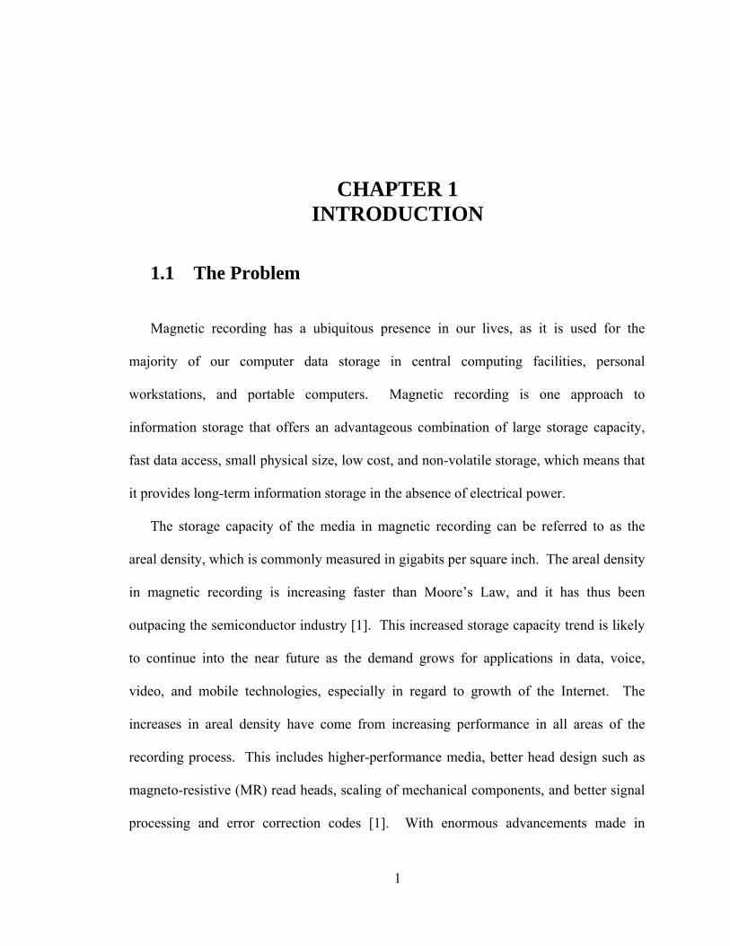
recorded bit density, or channel bit density, is related to the user density, , via
where r is the code rate. Figure 2.3 shows the transition response for some
values of D .
uD
/c uD D= r
)ka a −
D= ∗ −
c
-5 -4 -3 -2 -1 0 1 2 3 4 50
0.1
0.2
0.3
0.4
0.5
0.6
0.7
0.8
0.9
1
Tc
h(t)
Dc=1.0Dc=2.0Dc=3.0
Figure 2.3. Transition response, h t ( )
The encoded input data to the channel model, a , is a binary sequence having
-spaced discrete elements taking on the values . This sequence is written onto
the magnetic media by the write head using non-return-to-zero (NRZ) modulation that
creates a two-level transition sequence, c . This sequence written onto the media
contains transitions, which alternate in direction, wherever adjacent input elements differ
from each other ( . The transition sequence takes on the values 0 and
can be expressed as c a , where D is a T -second delay operator. Since
is a response to this transition sequence in the media, the continuous-time overall
k
1±cT
k
k ≠ , 2±1
(1 )k k c
( )h t
8

h
impulse response of the MRC, , also referred to as the dibit response, can be
expressed as
( )s t
. (2.3) ( ) ( ) ( )cs t h t h t T= − −
Figure 2.4 depicts the change in shape of as the value for changes. As the
density increases, the transition responses form closer together and thus cancel each other
out more, as observed in Figure 2.4. The frequency-normalized Fourier-transform (FT)
of the transition response, , equals
( )s t cD
( cH fT )
( )50( )
2cfT D
cH fT PW e ππ −= ,
)T
)
(2.4)
and from equation (2.3) and using FT relations, the frequency-normalized FT of the
overall impulse response, S f , can then be determined. Normalized versions of
for different values of D can be seen in Figure 2.5.
( c
( cS fT c
1
-5 -4 -3 -2 -1 0 1 2 3 4 5-1
-0.8
-0.6
-0.4
-0.2
0
0.2
0.4
0.6
0.8Dc=1.0Dc=2.0Dc=3.0
Tc
s(t)
Figure 2.4. Overall impulse response, ( )s t
9

1
The read-back signal can now be described as
, (2.5) ( ) ( ) ( )k ck
r t a s t kT n t∞
=−∞= − +∑
where the sequence is the encoded input data symbols and accounts for the
presence of additive noise. The block diagram for the entire MRC as an LTI system is
depicted in Figure 2.6. Noise in the MRC comes from many sources in the system, with
the major components of being media noise, electronics noise, off-track noise,
overwrite noise, and transition noise. In practice, it is common to approximate as
white noise, which generally reflects the aggregate noise relatively well [8,10].
ka ( )n t
( )n t
( )n t
For analysis purposes, it is more useful to work with a discrete-time model of the
magnetic recording channel. Using Berman’s model [8], which is equivalent to the
continuous-time model from an information transfer point of view, the coefficients of the
0 0.1 0.2 0.3 0.4 0.50
0.1
0.2
0.3
0.4
0.5
0.6
0.7
0.8
0.9Dc=1.0Dc=2.0Dc=3.0
fTc
Nor
mal
ized
Am
plitu
de
Figure 2.5. Normalized versions of ( )cS fT for different values of cD
10
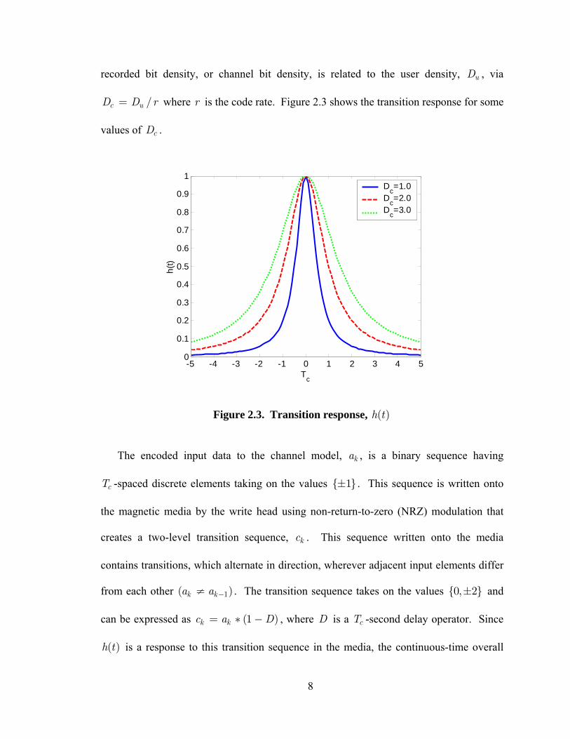
TransitionResponse +1 D−
( )h t
( )s t
( )r t
( )n t
kc ka
Figure 2.6. Magnetic recording channel
discrete-time transition response, , can be expressed as kg
( )( )
22
2tanh2 2
2
c
i c ck
c
DkE D D
gD
k
ππ
⎛ ⎞⎟⎜ ⎟+⎜ ⎟⎜ ⎟⎜= ⋅ ⎟⎜ ⎟⎟⎜ ⎟⎜ + ⎟⎜ ⎟⎝ ⎠
. (2.6)
With this equivalent, it is more convenient, both analytically and numerically, to work
with the discrete channel compared to the continuous-time channel. The analytical model
is now shown in Figure 2.7, where . ( ) (1 ) ( )f D D g D= −
+1 D− ( )g D
( )f D
kr
kn
kcka
Figure 2.7. Discrete-time magnetic recording channel
11

2.3 Optimum Detector
Viewing the magnetic recording system as a communications channel, an optimum
detection method can be determined. Making the assumption that the channel is LTI and
that it has additive white Gaussian noise (AWGN), then the optimum detector
corresponds to a sampled matched filter, , with a noise whitening filter and a
maximum likelihood sequence detector (MLSD) [11]. A diagram of this detector is
shown in Figure 2.8.
(- )s t
Figure 2.8. Optimal Detector
Channel MatchedFilter
NoiseWhitening
FilterMLSD+
1
cT
( )s t ( )s t−
( )r t ka ky ˆ ka
( )n t
The MLSD, which is known to achieve the best error-probability performance of all
existing equalizers and detectors, entails making a decision about the received data based
on all samples of the received sequence. Given a particular observed sequence, , the
MLSD seeks to choose the sequence, , that maximizes the conditional probability
ky
ˆ ka
ˆ( k kP y a ) . However, the high complexity of this brute force method of searching through
all possible transmitted sequences for a length L input sequence to the channel
generally renders this impractical for any reasonable length data sequence. Hence, for
channels with long ISI spans, the full-state MLSD serves only as a benchmark and is
rarely used.
2L
12

2.4 Partial Response
In practice, the number of states required in the MLSD for a recording channel and
matched filter will be prohibitive for complexity reasons. Consequently, sub-optimal
receivers such as symbol-by-symbol equalizers are widely used. When addressing the
ISI problem, linear equalizers are the simplest to implement and analyze. Although,
unlike MLSD, equalization enhances the noise.
A common practice in magnetic recording systems is to replace the combination of
the matched filter and whitening filter with a partial response equalizer, which shapes the
channel to appear to have a response with a shorter span [12]. The response that this PR
equalizer is attempting to shape the channel to is referred to as a target, which is often
described by a polynomial in terms of -second delay operators D . This equalization
process is deemed “partial response” seeing that it still allows ISI to be present; however,
this ISI is well defined and can be accounted for in the detection process. In contrast, a
“full response” equalizer is a type of equalizer that attempts to remove all the ISI. With a
PR equalizer, the amount of ISI is controlled in such a fashion that the target has a short
enough length such that detection may be performed with a manageable number of states
for state-based detectors.
cT
In magnetic recording systems, many targets have been deemed suitable for this PR
equalization process [13]. The Thapar-Patel class of partial responses consists of targets
of the polynomial form (1 where n is to increase with increasing
recording density. This class of targets is considered an appropriate choice for the MRC
)(1 )nD D− +
13

as the factor (1 provides a spectral null at DC similar to the frequency response of
the MRC. The (1 factor matches the high-frequency attenuation of the channel.
)D−
)nD+
A common target seen in magnetic recording research is the PR4 response. Using the
Thapar-Patel class of partial responses, the PR4 response can be defined as the target
given by , and thus the response can be written as . Using
, the frequency response is calculated as
24( ) 1 -PRH D D=1n =
- 2 cj fTD e π=
(2.7) 24( ) 4 sin( )cos( ) cj fT
PR c c cH fT j fT fT e ππ π −= .
.
) )
At higher recording densities, the extended PR4 target, EPR4, is considered more suitable
than the PR4 target. The EPR4 target, , is given by
and has the frequency response
24( ) (1 - )(1 )EPRH D D D= + 2n =
(2.8) 2 34( ) 8 sin( )cos ( ) cj fT
EPR c c cH fT j fT fT e ππ π −=
Increasing the value of n to 3 will provide the polynomial for the E2PR4 target.
The normalized frequency responses of and are shown in
Figure 2.9. Comparing the shape of these responses with the frequency response of the
MRC in Figure 2.5, it is evident that while the frequency responses of the PR channels do
approximate the real channel, they do not match it exactly. The better the target’s
response matches the channel response, the greater the reduction in noise enhancement
attained during equalization. Thus, the better the target is matched to the channel, the
better the detection performance. There has been some work on other appropriate targets
[14-16]; however, this work focuses on the PR4 and EPR4 targets because of their
ubiquity in magnetic recording research.
4(PR cH fT 4(EPR cH fT
14

1
2.5 Channel Detection with PR Equalization
Channel detection schemes often have complexities that are directly correlated to the
length of the channel impulse response. Nevertheless, with PR equalization, the channel
impulse response length is shortened so that it becomes feasible to use high-complexity
algorithms on this shortened impulse response. The total complexity is an important
issue in applications for magnetic recording channels, as they have constraints since
power dissipation has become a growing concern [17]. In this section, the Bahl-Cocke-
Jelinek-Raviv (BCJR) algorithm for use in channel detection on the MRC is highlighted;
however, some background on other schemes is also introduced.
0 0.1 0.2 0.3 0.4 0.50
0.1
0.2
0.3
0.4
0.5
0.6
0.7
0.8
0.9HPR4(fTc)HEPR4(fTc)
fTc
Nor
mal
ized
Am
plitu
de
Figure 2.9. Normalized frequency responses of 4( )PR cH fT and 4( )EPR cH fT
15

2.5.1 Complexity Considerations
Without PR equalization, the MRC theoretically has infinite length. With the PR
equalization, the channel impulse response is shortened to have length m , which creates
a manageable number of states, , for a trellis-based channel detector. It is the
number of states that directly affects the complexity for these detectors. PR equalization
gives the PR4 and EPR4 targets four and eight states, respectively. The full channel
theoretically has infinite support, but if it is approximated by selecting a finite number of
taps so that 99.6% of the energy is retained, this approximate impulse response will have
10 taps at a channel density . This number of taps will yield 1024 states, which
is regarded as impractically complex for real implementations.
12m−
2.5cD =
The number of states for the detector is governed by the channel’s trellis structure. A
trellis is an illustration of a finite-state machine’s (FSM) state diagram, but it explicitly
shows the passage of time. The states are determined by the memory elements of the
FSM, with each unique combination of the bits in the memory elements creating a new
possible state. For example, a binary FSM with two memory elements can have four
possible states, each associated with its contents (00), (01), (10), or (11). The trellis
structure for this example is displayed in Figure 2.10. In this diagram, it is assumed that
the FSM begins at state (00). Each branch in the trellis denotes a possible movement
from state s at time to state s at time k . The detector uses these possible state
transitions to determine the most probable input bits to the FSM.
′ 1k −
A certain number of computations are associated with each state in the trellis. So, as
the number of states increase, so does the overall complexity. With each new memory
16

(00)
(01)
(10)
(11)
k=0 k=1 k=2 k=3 k=4 ...
Discrete-time index
Stat
e in
dex
Figure 2.10. Example trellis diagram for a 4-state finite-state machine
element in the binary FSM, the trellis size doubles, which leads to a complexity that is
exponential in relation to the FSM’s memory length.
Having fewer states for the detector is important if this detector is utilizing an
algorithm such as the BCJR algorithm, which is a symbol-by-symbol maximum
a posteriori (MAP) algorithm that is optimal for estimating the states or outputs of a
Markov process in the presence of white noise [18]. A Markov process is a random
process whose future probabilities are determined by its most recent values. The BCJR
algorithm, which is detailed in the next subsection, has complexity that is exponential in
the length of the channel since it is a trellis-based algorithm. With a binary sequence of
length as the input to the channel, the BCJR has approximately real
additions and real multiplications [19]; this exponential complexity
illustrates why m should be small when using the BCJR algorithm.
1(10 2 )mL −⋅L
1(6 2 )mL −⋅
17

The true MAP algorithm presents technical difficulties because of numerical
representation problems, nonlinear functions, and a high number of additions and
multiplications. By shifting to the logarithmic domain, the Log-MAP algorithm [20]
does not have the numerical representation problems and changes some multiplications to
additions, which are inherently less complex in hardware implementation. The Log-
MAP algorithm is equivalent to the true MAP, but without some of the disadvantages.
Hence, this work considers only the logarithmic form of the MAP algorithm for
implementation purposes.
2.5.2 The BCJR Algorithm
The algorithm described in this section is the standard Bahl-Cocke-Jelinek-Raviv
algorithm from [18]. The motivation for describing this algorthim is that it is of interest
to see the performance of this classic algorithm compared with other types of channel
detectors on the system that is described in later chapters. But most important, some of
the presented work in Chapter 3 looks into modifying this algorithm for noise predition
purposes on the MRC.
In demonstrating the BCJR algorithm, the system is assumed to have binary
transmission of the coded bits where knowledge of the encoding trellis is known. For
a binary trellis, s is the state of the encoder at time k , and s is the state at time .
is the set of all ordered pairs ( , corresponding to all state transitions caused by
the channel input . S is defined in a similar manner for .
ka
′ 1k −
S+ )s s′
−1ka = + 1ka = −
The main goal of the BCJR algorithm operating as a channel detector is to compute
a posteriori probabilities (APP) of the coded input of the channel. This is done based a
18

on knowledge of the trellis, the a priori probabilities of the channel inputs, and the
channel output . Let and . The
BCJR algorithm assigns if , or it assigns
otherwise. More concisely, the decoder’s decision is identified as
r 0 1 2[ , , , ... ]La a a a=a 0 1 2 1[ , , , ... ]L mr r r r + −=r
( 1 | ) ( 1 |k kP a P a= + > = −r rˆ 1ka = + )
ˆ 1ka = − ka
, (2.9) ˆ sign( )k ka L=
where is referred to as the log-likelihood ratio (LLR), defined as kL
( 1 |log
( 1 |k
kk
P aL
P a⎛ ⎞= + ⎟⎜≡ ⎟⎜ ⎟⎜⎝ = −
rr))⎠
. (2.10)
From Bayes’ rule, the LLR can be written as the sum kL
( | 1) ( 1)log log
( | 1) ( 1)k k
kk k
P a P aL
P a P a⎛ ⎞ ⎛= + = +⎟ ⎟⎜ ⎜= +⎟ ⎟⎜ ⎜⎟ ⎟⎜ ⎜⎝ = − ⎠ ⎝ = −
rr
⎞⎠
, (2.11)
where the first term corresponds to what is known as the extrinsic information, , and
the second term corresponds to the a priori LLR, . Using the trellis, may be
written as
kλ
pkλ kL
1
1
( , , )log
( , , )
k kS
kk k
S
p s s s s pL
p s s s s p+
−
−
−
⎛ ⎞′= = ⎟⎜ ⎟⎜ ⎟⎜= ⎟⎜ ⎟′= =⎜ ⎟⎟⎜ ⎟⎜⎝ ⎠
∑∑
r r
r r
( )
( ) . (2.12)
Notice that the term may be cancelled. The joint probability can be
written as the product of three independent probabilities:
( , , )p s s′ r( )p r
1
( , , ) ( , ) ( , |s ) ( | )
( , ) ( | ) ( | , ) ( | )
( ) ( , ) ( )
j k k j k
j k k j k
k k
p s s p s p s r p s
p s P s s p r s s p s
s s sα γ β
< >
< >
−
′ = ′ ⋅ ′ ⋅
= ′ ⋅ ′ ⋅ ′ ⋅
= ′ ⋅ ′ ⋅
r r r
r r
k s
. (2.13)
Equation (2.12) can then be rewritten as
19

1
1
( ) ( , ) ( )log
( ) ( , ) ( )
k k kS
kk k k
S
s s s sL
s s s s
α γ β
α γ β+
−
−
−
⎛ ⎞′ ′ ⎟⎜ ⎟⎜ ⎟⎜= ⎟⎜ ⎟′ ′⎜ ⎟⎟⎜ ⎟⎜⎝ ⎠
∑∑
. (2.14)
The can be computed in a forward recursion as ( )k sα
(2.15) 1( ) ( ) ( , )k k ks S
s sα α γ−′∈
′ ′= ∑ s s
0
k s s
0
with initial conditions and . These initial conditions express
that it is expected that the encoder starts in state 0. The probabilities are computed
in a backward recursion as
0(0) 1a = 0( 0)a s ≠ =
( )k sβ
, (2.16) 1( ) ( ) ( , )k ks S
s sβ β γ−∈
′ ′= ∑
and if it is expected that the encoder ends in state 0 after input bits (implying
that appropriate termination bits are selected), the boundary conditions are
and .
1L m+ −
1(0) 1L mβ + − = 1( 0)L m sβ + − ≠ =
In both the forward and backward recursions, the branch transition probabilities
are needed, which can be written as ( , )k s sγ ′
. (2.17) 1
1 1
( , ) ( , | )
( | , )Pr( | )
k k k k
k k k k k
s s p s s r s s
p r s s s s s s s s
γ −
− −
′ ′= = =
′ ′= = = = =
The second term in equation (2.17) is the a priori probability that the coded bit, ,
is the input that caused the transition from state s to state s . Assuming AWGN with
variance , the branch transitions may be reduced to
thk ka
′
2σ
2( , )
1 22
1( , ) Pr( | ) exp
22
s sk
k k k
r rs s s s s sγ
σπσ
′
−
⎡ ⎤−⎢ ⎥′ ′= = = ⋅ −⎢ ⎥⎢ ⎥⎣ ⎦
, (2.18)
20

where the expected noiseless observed output that corresponds to the transition along that
branch resulting from the channel input bit is denoted by . For a BPSK alphabet
where the a priori information is given in the LLR form , the a priori probability can
be written as
( , )s sr ′ka
pkλ
/2( , )
1
( , )
Pr( | ) exp( /2)1
exp( /2)
pk
pk
ps sk k k
ps sk k
es s s s r
e
A r
λ
λ λ
λ
−′
− −
′
⎛ ⎞⎟⎜′ ⎟= = = ⋅⎜ ⎟⎜ ⎟+⎝ ⎠
=
. (2.19)
The term will cancel in (2.12), as it is independent of . kA ka
2.5.3 State-of-the-Art Channel Detection in Magnetic Recording
As previously mentioned, the magnetic recording channel will appear to the detector
to have only a few states when using PR equalization, thus making it feasible to use the
BCJR algorithm. The output of the detector is then given to a decoder, assuming that the
system is applying error-correction coding (ECC). A system with ECC, an interleaver π ,
the MRC, PR equalization, a BCJR channel detector for the PR target, and a deinterleaver
is illustrated in Figure 2.11. A turbo code implementation of this system has been
studied by other authors [21,22]; however, they execute the BCJR channel detection
assuming the noise in the detector to be white after PR equalization, which is not the
most accurate representation for this case. There is a performance loss by disregarding
the correlation in the noise.
1π−
There has been some work on using algorithms for the channel detector that account
for the noise correlation resulting from the PR equalization process. This previous work
has focused on modifying the BCJR algorithm with an extended trellis for correlated
21

PREqualization
Filter
ChannelDetector(BCJR)
noise [5-7]. Although gains of about 1 dB may be observed with this approach, the added
complexity is considerable because of the extended trellis. To account for correlated
noise by using additional memory with a length 2, the trellis size is quadrupled, thus
quadrupling the complexity.
In addition to the work with the BCJR with an extended trellis, there has been
research that has focused on noise-predictive maximum-likelihood (NPML) detectors
[23-25]. These detectors embed a noise prediction/whitening process into the branch
metric computations of the Viterbi algorithm [26]. NPML provides performance gains
over PRML detectors and is considered the current state-of-the-art in magnetic recording.
2.6 Turbo Equalization
In the system demonstrated in Figure 2.11, the channel detector is implemented only
once for each sector. Yet, if the decoder provides soft information about the bits to the
detector in an iterative process, also referred to as turbo equalization, a significant
amount of coding gain may be attained, though at the added expense of complexity. By
applying turbo equalization methods to this system on the MRC, there are better
performance benefits that can be attained [21, 27, 28].
Figure 2.11. System diagram with encoder, MRC, PR equalizer, BCJR channel detector, and decoder
OuterCode MRC Decoder
ka kr ˆ ka kxπ
ˆ kx1π−
22

Turbo equalization is an iterative joint equalization and decoding process first
introduced in a general way in [29], and it was shown to almost completely mitigate the
ISI effects in certain circumstances. The goal of equalization is to minimize the ISI
distortion at the receiving filter output and reduce the system’s bit error rate (BER).
Turbo equalization is a solution to this ISI distortion problem that considers the channel
memory effect and uses it as a type of time diversity. In this approach, the discrete-time
channel model can be seen as a convolution encoder with rate 1 and therefore can be
interpreted as a Markov chain with its behavior being represented by a trellis
diagram [30]. Fundamentally, turbo equalization treats the ISI trellis as an inner
constituent encoder in serial concatenation with the outer code, such as a convolutional
code or turbo code. From this viewpoint of considering the channel as an encoder, the
turbo equalizer attempts to “decode” the received signal.
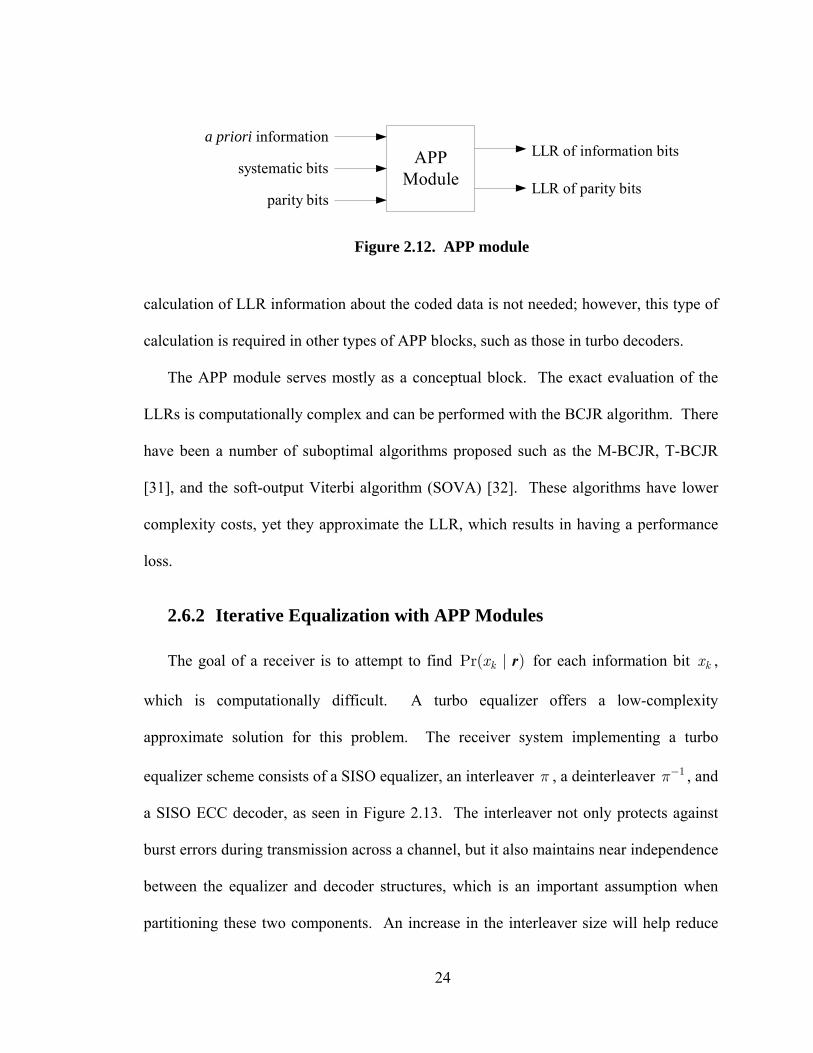
2.6.1 The APP Module
Before continuing at this point, an APP module should first be defined. This needs
be done because an APP module is the core building block of a successful iterative
receiver. An APP module, as shown in Figure 2.12, is a soft-input soft-output (SISO)
block that calculates a posteriori probabilities of the information bits and parity bits. The
inputs to this module include the systematic bits, the coded bits, and any a priori LLR
information from the previous block or iteration. The APP module then outputs the LLR
information about the input data as well as the LLR information about the parity data.
For the case of channel detection, not all of these inputs and outputs are used. When
ISI is present, there are no systematic bits available to the receiver. In addition, the
23
APPModulesystematic bits
parity bits
a priori informationLLR of information bits
LLR of parity bits
Figure 2.12. APP module
calculation of LLR information about the coded data is not needed; however, this type of
calculation is required in other types of APP blocks, such as those in turbo decoders.
The APP module serves mostly as a conceptual block. The exact evaluation of the
LLRs is computationally complex and can be performed with the BCJR algorithm. There
have been a number of suboptimal algorithms proposed such as the M-BCJR, T-BCJR
[31], and the soft-output Viterbi algorithm (SOVA) [32]. These algorithms have lower
complexity costs, yet they approximate the LLR, which results in having a performance
loss.
2.6.2 Iterative Equalization with APP Modules
The goal of a receiver is to attempt to find Pr( for each information bit ,
which is computationally difficult. A turbo equalizer offers a low-complexity
approximate solution for this problem. The receiver system implementing a turbo
equalizer scheme consists of a SISO equalizer, an interleaver , a deinterleaver , and
a SISO ECC decoder, as seen in Figure 2.13. The interleaver not only protects against
burst errors during transmission across a channel, but it also maintains near independence
between the equalizer and decoder structures, which is an important assumption when
partitioning these two components. An increase in the interleaver size will help reduce
| )kx r kx
1π−π
24

APPEqualizer
the correlations between the coded bits, which results in the system performance having a
dependency on the interleaver size.
Using APP modules, the SISO equalizer block uses the received signal from the
channel and the a priori information given to it from the decoder for its inputs. For the
first iteration, there is generally no a priori information available. Since the equalizer is
working over a channel with ISI, the received symbols serve as parity information only,
as there is no systematic data accessible to the receiver. The equalizer calculates the LLR
of the coded channel bits with only the knowledge of the channel. At this stage, ECC
is ignored. From the viewpoint of the APP module, the input is only information
symbols, as it does not contain redundancy. Therefore, the channel detector does not
compute any parity LLR. The extrinsic part of the LLR information data is then
deinterleaved and is transferred to the decoder.
ka
Figure 2.13. The turbo equalization process as an iterative loop
APPDecoder
a prioriinformation
OutputDecision
ChannelOutput
a posterioriinformation
1π−π
25

The decoder then takes this LLR information and uses it as the systematic and parity
inputs to its APP module. Again, for the first iteration, there is generally no a priori
information available for the decoder. The decoder ignores the ISI and assumes that the
equalizer has removed all of its effects. Finally, the decoder exploits the knowledge of
the code structure and computes new LLRs of each coded symbol. The extrinsic part of
this LLR data is then interleaved and given to the equalizer as a priori information for the
next iteration.
It is important that only the extrinsic part of the APP information be fed to the next
channel detector. The other part of the APP data is the a priori information, which is
already known to the detector, as it was the module that gave the decoder that
information. The equalizer assumes that the a priori data it is given from the decoder is
extra information about the channel bits gleaned only from exploiting the code structure.
So, subtracting the a priori information from the full LLR information will prevent
positive feedback of information back to the equalizer.
The performance of the turbo equalizer is directly related to the number of
iterations [29]. Turbo equalization also experiences a trigger point followed by a
breakdown effect, that is, the performance gets better for each iteration if the probability
of error of the first iteration is lower than the trigger point [33]. This iteration
performance underscores the motivation for turbo equalization. At low SNR, the BER is
dominated by the convergence of the iterative equalization and decoding process. For
this reason, codes designed to improve the convergence can outperform those codes that
are designed to optimize the asymptotic performance with ML decoding [34].
26
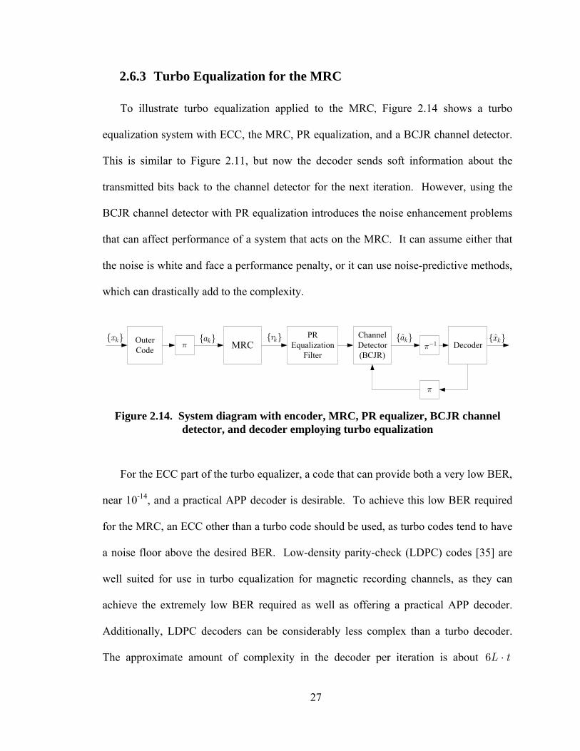
2.6.3 Turbo Equalization for the MRC
To illustrate turbo equalization applied to the MRC, Figure 2.14 shows a turbo
equalization system with ECC, the MRC, PR equalization, and a BCJR channel detector.
This is similar to Figure 2.11, but now the decoder sends soft information about the
transmitted bits back to the channel detector for the next iteration. However, using the
BCJR channel detector with PR equalization introduces the noise enhancement problems
that can affect performance of a system that acts on the MRC. It can assume either that
the noise is white and face a performance penalty, or it can use noise-predictive methods,
which can drastically add to the complexity.
Figure 2.14. System diagram with encoder, MRC, PR equalizer, BCJR channel detector, and decoder employing turbo equalization
OuterCode MRC
PREqualization
Filter
ChannelDetector(BCJR)
Decoder ka kr ˆ ka
π kx ˆ kx1π−
π
For the ECC part of the turbo equalizer, a code that can provide both a very low BER,
near 10-14, and a practical APP decoder is desirable. To achieve this low BER required
for the MRC, an ECC other than a turbo code should be used, as turbo codes tend to have
a noise floor above the desired BER. Low-density parity-check (LDPC) codes [35] are
well suited for use in turbo equalization for magnetic recording channels, as they can
achieve the extremely low BER required as well as offering a practical APP decoder.
Additionally, LDPC decoders can be considerably less complex than a turbo decoder.
The approximate amount of complexity in the decoder per iteration is about 6 L t⋅
27

LDPCHmultiplications and 5 additions. Here t is the column weight of L t⋅ , the parity
check matrix of the code. LDPC codes, first introduced in 1962, were largely forgotten
until a recent paper by MacKay demonstrated that their performance is almost as close to
the Shannon limit as turbo codes [36].
28

CHAPTER 3 THE NOISE-PREDICTIVE BCJR ALGORITHM
3.1 Introduction
The standard approach to equalization in magnetic recording is the PRML strategy,
where the front-end filter transforms the underlying channel to a target partial response,
which has little memory. With this strategy, the length of the impulse response is
shortened so that trellis-based channel detection may be performed with a manageable
number of states. Unfortunately, the front-end filter introduces significant performance
penalty because of noise enhancement and correlation.
Much of the previous work on the magnetic recording channel has implemented
detectors over the ideal PR channel with the assumption that the noise is not correlated.
Instead, those detectors use the Euclidian distance metric, which is optimal only for the
white Gaussian noise case. Appling such detectors over the more realistic channel with
the colored noise will definitely impair performance [22,37].
There have been a few different approaches on how to manage the colored noise seen
at the detector. Some work has focused on modifying the BCJR algorithm with an
extended trellis to incorporate the correlated noise [5-7], where the calculation of the
branch metrics is based on the assumption that the noise is either a Gaussian-Markov or
Gaussian random process. With this approach of extending the trellis for the correlated
29

noise, gains can be observed, but there is added complexity because the larger sized
trellis. In order to account for noise with a memory of length 2, the trellis size is
quadrupled, thus quadrupling the complexity. Further research has focused on NPML
detectors [23-25]. These detectors embed a noise prediction/whitening process into the
branch metric computations of the Viterbi algorithm and provide performance gains over
the PRML detectors.
In this chapter, a new soft-output detection strategy is presented that mitigates colored
noise in partial-response (PR) equalized magnetic recording channels. The algorithm can
be viewed as a marriage of the traditional BCJR algorithm with the notion of survivors
and noise prediction. This new algorithm performs comparably with previously reported
BCJR-based techniques, but is significantly less complex because it does not require an
extended trellis.
3.2 Noise Correlation
As it is well known, the process of partial-response equalization causes the noise seen
at the detector to be correlated [13]. Let be the D -transform input to the MRC as
seen in Figure 3.1, and let be the target response. The output of the PR filter,
, is given by
( )a D
( )PRg D
( )y D
. (3.1) ( ) ( ) ( ) ( )PRy D a D g D w D= +
Here represents the total distortion, which is the colored noise plus any residual
interference.
( )w D
30

The zero-forcing (ZF) finite impulse response equalizer, , which shapes the
channel to the desired target response is given by
( )c D
( )( )
( )PR
f
g Dc D
R D= , (3.2)
where is the -transform of the discrete-time channel autocorrelation
coefficients. In a zero-forcing formulation, the noise sequence seen at the channel
detector is a filtered version of the AWGN . The autocorrelation function of this
colored noise sequence is
( )fR D D
( )w D
( )n D
1( ) ( )
( )( )
PR PRw o
g D g DR D N
−=
fR D . (3.3)
0N is the power spectral density of the AWGN. The power spectral density (PSD) of the
filtered noise sequence is simply the Fourier transform of . ( )wR D
For the minimum mean square-error (MMSE) case, the infinitely long PR equalizer is
given by [38]
2
2( )
( )( )a PR
a f o
g Dc D
R D Nσ
σ=
+ (3.4)
+( )f D( )r D
( )n D
( )a D1( )f D− ( )c D
( )y D
Figure 3.1. The MRC with the discrete-time model, the matched filter, 1( )f D− , and the PR equalizer, ( )c D
31

where is the average symbol energy of the sequence . In this formulation,
represents the filtered noise sequence as well as a residual interference component. The
autocorrelation function for the total distortion in this MMSE formulation is given by
2aσ ( )a D ( )w D
2 1
2( ) ( )
( )( )
a PR PRw o
a f o
g D g DR D N
R D Nσσ
−=
+ . (3.5)
To demonstrate these formulations, two plots are presented for the case of a PR4
target, , and . Figure 3.2 displays the frequency response of the PR
equalizers for the ZF and MMSE formulations from
2.0cD = 0.08oN =
(3.2) and (3.4) respectively. Note
that in these equations, does not include the matched filter . It should be
noted that since the matched filter has a zero at DC, the concatenation of these two filters
1(f D−( )c D )
will negate what appears to be infinite gain at DC for the ZF equalizer. Figure 3.3
Figure 3.2. The frequency response of the PR equalizers for the ZF and MMSE formulations with 2.0cD = , 0.08oN = , and using the PR4 target
32
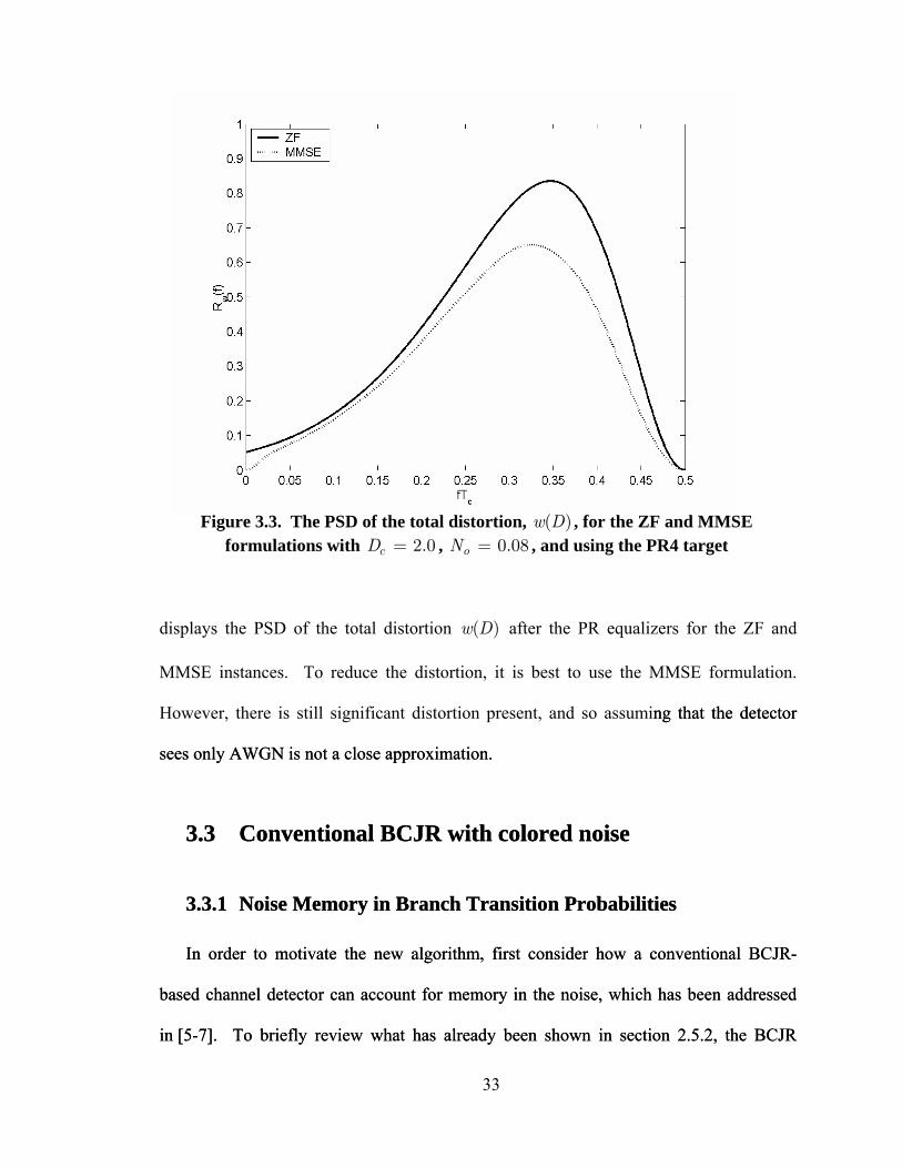
Figure 3.3. The PSD of the total distortion, ( )w D , for the ZF and MMSE formulations with 2.0cD = , 0.08oN = , and using the PR4 target
displays the PSD of the total distortion ( )w D after the PR equalizers for the ZF and
MMSE instances. To reduce the distortion, it is best to use the MMSE formulation.
However, there is still significant distortion present, and so assuming that the detector
sees only AWGN is not a close approximation.
ng that the detector
sees only AWGN is not a close approximation.
3.3 Conventional BCJR with colored noise
3.3.1 Noise Memory in Branch Transition Probabilities
ntional BCJR-
bas
3.3 Conventional BCJR with colored noise
3.3.1 Noise Memory in Branch Transition Probabilities
ntional BCJR-
bas
In order to motivate the new algorithm, first consider how a conveIn order to motivate the new algorithm, first consider how a conve
ed channel detector can account for memory in the noise, which has been addressed
in [5-7]. To briefly review what has already been shown in section 2.5.2, the BCJR
ed channel detector can account for memory in the noise, which has been addressed
in [5-7]. To briefly review what has already been shown in section 2.5.2, the BCJR
33
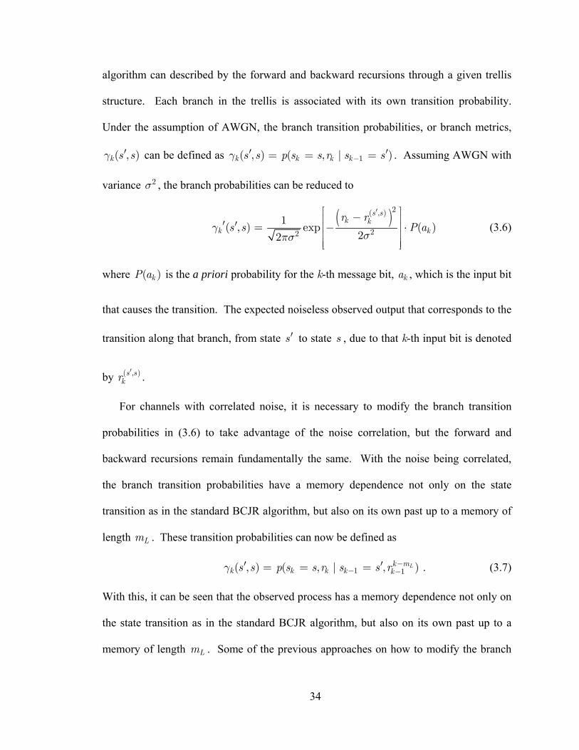
algorithm can described by the forward and backward recursions through a given trellis
structure. Each branch in the trellis is associated with its own transition probability.
Under the assumption of AWGN, the branch transition probabilities, or branch metrics,
( , )k s sγ ′ can be defined as 1( , ) ( , | )k k k ks s p s s r s sγ −′ ′= = = . Assuming AWGN with
2σ , the branch probabilities can be reduced to variance
(
)2( , )
22( , ) exp ( )
22
s sk
k k
rs s P aγ
σπσ
′1 kr
⎡ ⎤′ ′ = − ⋅⎢ ⎥
⎢ ⎥
−⎢ ⎥
⎢ ⎥⎣ ⎦
(3.6)
where is the a priori probability for the k-th message bit, , which is the input bit
by .
For channels with correlated noise, it is necessary to modify the branch transition
pro
( )kP a ka
that causes the transition. The expected noiseless observed output that corresponds to the
transition along that branch, from state s′ to state s , due to that k-th input bit is denoted
( , )s s′kr
babilities in (3.6) to take advantage of the noise correlation, but the forward and
backward recursions remain fundamentally the same. With the noise being correlated,
the branch transition probabilities have a memory dependence not only on the state
transition as in the standard BCJR algorithm, but also on its own past up to a memory of
length Lm . These transition probabilities can now be defined as
1 1( , ) ( , | , k mk k k k )Lk . (3.7)
With this, it can be seen that the observed process has a memory dep ence not on
s s p s s r s s rγ −− −′ ′= = =
end ly on
the state transition as in the standard BCJR algorithm, but also on its own past up to a
memory of length Lm . Some of the previous approaches on how to modify the branch
34
metrics to combat the colored noise differed on their assumptions that either the noise is
based on a Gaussian-Markov random process or a Gaussian random process [5-7]. Yet,
each of these modified BCJR algorithms makes use of an extended trellis. Given that the
channel impulse response has a length m , the trellis is extended from 12m− states to
12 Lm m− + states. The value used for Lm ay be chosen to be a smaller value than the
gth of the noise memory in order to maintain a reasonable number of states in
the trellis. By the use of a smaller value for Lm , there is a tradeoff between performance
and complexity.
m
actual len
3.3.2 Linear Prediction
th correlated is to use linear prediction, whereby a
line
PR-equa el output is kr r w′ , where
pre
)
L
k k k k k i ii
ms s s s
k k i ik k ii
e w
r r r r p
−=
′ ′− −
== − − −∑
. (3.8)
One idea to mitigate distortion at is
ar combination of past noise distortion samples are used to predict the next noise
sample. Motivated by a similar linear prediction approach found in the derivation for
NPML, this section describes a method that uses a whitening filter in its noise prediction
for a BCJR-based algorithm.
Let it be assumed that the ( , )s sk k= +lized chann
kw represents the total distortion. The power of this distortion can be reduced by linear
diction [39]. Let 11( ) ( ... )L
L
mmp D p D p D= + + be the transfer polynomial of an
Lm -tap MMSE predic r operating on the noise sequence
produce the estimate ˆkw . The prediction error sequence is then given by
Lm
w w w p= − = −∑
tor of kw . The linear predicto
will
1
( , ) ( , )
1
ˆ
( ) (
35

This prediction error is equivalent to the whitened distortion component of the PR-
equalized sample . The optimum predictor that minimizes the mean-square error
is given by [23]
kr
2| |keEε =
0
( )q Dq
⎛ ⎞⎜ ⎟⎝ ⎠
( the minimum phas
( ) 1p D ⎟⎜= − − ⎟ , (3.9)
where is e causal factor of .
From the noise prediction viewpoint, the branch metric can be modified to
)q D 1/ ( )wR D
( )2( , )
2 2
( , ) exp2
k s sγπσ
ˆ1( )
2
s sk kk
k
r r wP a
σ
′⎡ ⎤− −⎢ ⎥′ ⋅⎥
= −⎢ ⎥⎢⎢ ⎥⎣ ⎦
. (3.10)
Not predicted
value would be zero. Thus, (3.10) would reduce back to (3.6). Assum
is equalizing to the PR4 target, the expected noiseless observed output is writte
k kk − k−
etric
ˆ ( ) ( ) ( )m
s sk k k k k k i k i k i ikr r w r a a s r a s a s p′
− − − − −′ ′− − = − + − − +∑ . (3.11)
c determined by (3.11) is not suitable for high-speed
implementation [24]. This is because of its requiring several multiplications rather than
additions and random-access memory (RAM) lookup. Fortunately, this structure can be
k k k k k i iki
−=
ice that if the distortion w is AWGN, it would not be correlated and thek
ing that ( )c D ˆkw
n as
( , ) ( )s sr a a s′ ′= − , where the bit ( )a s′ is determined by the hypothetical state that
the transition originated from. Given the original PR4-based trellis, the branch m
can now by revised by using
1
L
i=
′
However, the branch metri
22
( )( , )2 2
made suited for RAM based implementation by rearranging (3.11) as
2
( , )Lm
s sr r w v a a s b+
′ ′− − = − + ∑ , (3.12) 1
ˆ ( )
36

where 1Lm
k k k i iiv r r p−=
= −∑ is the output of the prediction error filter [1 ( )]p D− . The
coefficients are determined by the polynomial ib
[ ]
11 2
2
( ) (1 )
(1 ) 1 ( )
LL
mmb D b D b D
D p D
++= − − −
= − −
2
. (3.13)
It should be noted that with this method, the effective ISI memory for the PR4-based
o r than 2 for the original PR4 trellis with
the AWGN assumption. A less complex algorithm is desired for any practical
application.
3.4 Noise-Predictive BCJR
R extended trellis approach to the noise correlation does work well and
provides performance gains over the standard BCJR algorithm that operates on the
AW s otivated to find a sub-optimal method to
combat the noise correlation without extending the trellis. The idea is to marry the idea
of n
trellis with n ise prediction is now 2+ , ratheLm
The BCJ
GN a sumption, but this research is m
oise prediction with the notion of survivors. In the algorithm presented here, not all
noise samples are directly available to the algorithm, but it is a simple matter to introduce
a survivor path for each node of the trellis, and to use the symbols in the survivor history
to help predict the noise. This new noise-predictive BCJR (NP-BCJR) algorithm
performs comparably with previously reported BCJR-based techniques, but is
significantly less complex because it does not require an extended trellis.
In order to demonstrate this new method, the calculation in (3.10) will be
reexamined. Recall that the transition information ( , )s sr ′ is determined from a linear k
37

combination of the values 1 2, , ,k k ka a a− − … depending on the target response; e.g., for a
PR4 response, ( , )2( )s s
k kr a a s′− ′= − . To ascertain the past information ( , )s s
k ir′
− , 0i > , k
the past values are generally not accessible to the original PR4
trellis at time k since the four states mation on and . To
determine the value of the pas ssage bits not available to the original trellis, these bits
are estimated based on llis transitions. Thus, the branch transition
now wr s
2 21
ˆ ˆ ˆ( ) ( ) ( )k k k k k k i k i iki
r r w v a a s a s a s p− − − −=
− − = − + + −∑ , (3.14)
where the a s′ , , represent the estimated past message bits. Rather than increase
ation, as in the previous section,
this noise-predictive algorithm looks back through the trellis and finds the most likely
past states based on current state calculations. In other words, in addition to the forward
ard m trics o
backwards through the trellis that provides the most likely past
stat prem
( )k ia s− ′ and 2( )k ia s− − ′
only give infor 1( )ka s− ′ 2( )ka s− ′
t me
past likely tre
probabilities are itten a
( , )Lm
s s′ ′ ′ ′
l
the size of the trellis to determine this past state inform
( )
l m>ˆ ( )
and backw e f the original BCJR algorithm, the NP-BCJR maintains a set of
survivor paths for each node in the trellis in order to perform the linear prediction of the
total distortion.
So that the ˆ ( )la s′ can be estimated, the trellis has the same structure as in the general
PR4 case, but with survivor history information stored at each state as the NP-BCJR
algorithm moves forward through the trellis. This extra information will be a survivor
path memory looking
es given the ise that this path must end at state s at time k . The estimated past
38
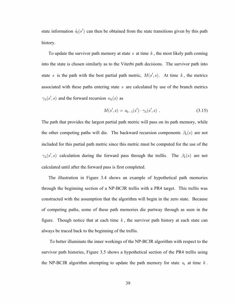
state information ˆ ( )la s ′ can then be obtained from the state transitions given by this path
history.
To update the survivor path memory at state s at tim k , the m st likely path coming
into the state is ch similarly as to the Viterbi path decisions. The survivor path into
state s i
e o
s the path with the best partial path m tric, . At time , the metrics
asso
( , )k k s s− ′
th m
the othe The backward recursion components are not
included for this partial path metric since this metric must be computed for the use
through
egin in the zero state. Because
of
th memory for state at time .
osen
e ( , )M s s′ k
ciated with these paths entering state s are calculated by use of the branch metrics
( , )k s sγ ′ and the forward recursion ( )k sα as
( , ) ( )M s s a s γ′ ′= ⋅ . (3.15)
The path that provides the largest partial pa etric will pass on its path memory, while
r competing paths will die.
1
( )k sβ
of the
( , )k s sγ ′ calculation during the forward pass through the trellis. The ( )k sβ are not
calculated until after the forward pass is first completed.
The illustration in Figure 3.4 shows an example of hypothetical path memories
the beginning section of a NP-BCJR trellis with a PR4 target. This trellis was
constructed with the assumption that the algorithm will b
competing paths, some of these path memories die partway through as seen in the
figure. Though notice that at each time k , the survivor path history at each state can
always be traced back to the beginning of the trellis.
To better illuminate the inner workings of the NP-BCJR algorithm with respect to the
survivor path histories, Figure 3.5 shows a hypothetical section of the PR4 trellis using
the NP-BCJR algorithm attempting to update the pa kbs
39

(00)
(10)
(01)
(11)
k=0 k=1 k=2 k=3 k=4
Discrete-time index
Stat
e in
dex
k=5 ...
Figure 3.4. Hypothetical survivor path memories in a section of the trellis using the NP-BJCR with a PR4 target
Bef
m
e
c bM s s′
ore the path memory can be updated, all the transition probabilities ( , )k s sγ ′ are
calculated. The transition probability ( , )k a bs sγ ′ is calculated with the knowledge of
as well as the estimated value based on the survivor path memory at
state ′ at time 1k − . More estimated values of ˆ ( )′ may be used, depending on what
value of is chosen to be implemented. A si ilar process is completed to compute
. To determine which path will its memory to state , the branch that
has th largest al path metric will survive; i.e., the NP-BCJR will compare
1( , ) ( ) ( , )a b k a k a bM s s s s sα γ−′ ′ ′⋅ to the value received by the calculation
1( ) ( , )k c k c bs s sα γ− ′ ′= ⋅ . The algorithm will update all survivor histories ending
at time k before continuing to the next trellis section.
2( )k aa s− ′ 3ˆ ( )k aa s− ′
as l aa s
Lm
( , )k c bs sγ ′ pass on bs
parti
=
( , )
40

cs ′
bs
( , )k a bs sγ
′
( , )k c bs s
γ ′
as ′
bs ′
ds ′
1k −
ds ′′
cs ′′
bs ′′
as ′′
(11)
(01)
(10)
(00)
2( )k ca s− ′
2( )k aa s− ′
3ˆ ( )k ca s− ′
3ˆ ( )k aa s− ′
kFigure 3.5. Hypothetical state transitions in a section of the trellis using
the NP-BJCR with a PR4 target
The NP-BCJR algorithm can
accordingly initialize the survivor path memory
calculate for all valid transitions using .14)
.15) for all valid transitions as in
by means
end traverse backwards to calculate the ’s using (2.16) deter
The res hm i o
e com n vers . Recall from the previous section
be described by the following pseudocode:
initialize 0( )sα and ( )L sβ for all s
for k=1:L, ( , )k s sγ ′
(3calculate ( )k sα for all s using (2
( , )kM s s′compute (3.15)
update the survivor histories at each of comparing the ( , )M s s′
s
k
( )k sβmine the LLR kL with (2.14)
ulting added complexity over the classic BCJR algorit s minimal compared t
th plexity required by the exte ded trellis ion
41

that as Lm increases, so does the number of states in the trellis for the BCJR with trellis
extension for colored noise. In contrast, the NP-BCJR algorithm uses an Lm -length
survivor history that does not require the trellis size to increase. There is the extra
storage requirement for the survivor paths through the trellis. For every valid transition,
there is one multiply for computing the partial path metric, and there are 12m−
comparisons at each stage. Recall that the extra computation required to find ˆkw for
( , )k s sγ ′ can be implemented by RAM lookup. These complexity calculations show that
the NP-BCJR algorithm is efficient in terms of extra computations required. The BER
ance of this new algorithm is illustrated in the next section.
3.5 Results
perform
re nel with AWGN equalized to a PR target with colored noise is
considered. The data is protected by a rate-8/9 (4095,3640) regular LDPC code with
colu
compa rf
ualization iterations. In Figure 3.7, the BER performances of the respective
algorithms are given, and the algorithms implementing the whitening filter are run with
A Lo ntzian chan
mn weight 3, and it is decoded using message passing and turbo equalization. The
SNR that is referred to in this section is defined as /i oE N where iE is the amount of
energy in an isolated transition pulse as defined in section 2.2. The system model is
shown in Figure 3.6, and was used in experiments to re the pe ormance between
the classic BCJR, the extended trellis BCJR, and the NP-BCJR algorithms as the channel
detectors.
The first set of results was attained with a channel density of 2.0, a PR4 target, and
five turbo eq
42

either or . The results show that the NP-BCJR algorithm for
has a 1 dB gain over the BCJR algorithm that ignores the noise coloration and a loss of
only 0.4 dB loss over the algorithm that extends the trellis; however, as mentioned
n.
the BER
performance of the respective BCJR algorithms discussed previously. In this setup, the
Figure 3.6. System model with turbo equalization over the magnetic recording channel
1Lm = 2Lm = 2Lm =
before, the NP-BCJR does require less complexity than the extended trellis versio
The complexity tradeoff given by the NP-BCJR is displayed in Figure 3.8, which
plots complexity (as measured by the number of operations per bit) versus the SNR
required to achieve a BER of 10-5. Each curve has five points, one for each of five
iterations of the turbo equalizer. In all curves, as the number of iterations increase, the
required amount of SNR will decrease, but in decreasing amount of performance gain.
There is a favorable performance-complexity trade-off for the NP-BCJR from Figure 3.8.
If only one iteration of the extended-trellis algorithm is considered, a turbo equalizer
based on the NP-BCJR algorithm can perform three iterations and require the same
amount of complexity, while simultaneously achieving an SNR gain of 0.3 dB.
The next set of results is from simulations with the same system model but with
channel density 2.5 and using the EPR4 target. Again, five turbo equalization iterations
are assumed. Only results for 2Lm = are plotted. Figure 3.9 shows
+ 1( )f D−( )f D
( )n D
ˆ ka kaEncoder Decoder( )c D Channel
Detector
43

Figure 3.7. BER performance of the classic BCJR, extended trellis BCJR, and the NP-BCJR for channel density 2.0, PR4
NP
the
-BCJR algorithm has a 1.4 dB gain over the classic BCJR algorithm that ignores the
noise correlation, but it has a loss of 0.3 dB from the algorithm with the extended trellis.
The value of the NP-BCJR is vividly illustrated in Figure 3.10, which plots the
complexity versus required SNR to attain a BER of 10-5 for each turbo equalization
iteration. Here it can be seen that the NP-BCJR has a favorable performance-complexity
trade-off. While each iteration of the NP-BCJR algorithm performs slightly worse than
extended-trellis algorithm, its low complexity allows for a larger number of turbo
equalization iterations. For example, consider two iterations of a turbo equalizer based
on the extended-trellis algorithm. From Figure 3.10, a turbo equalizer based on the
NP-BCJR algorithm could perform three iterations and still be 15% less complex, while
simultaneously achieving an SNR gain of 0.3 dB.
44

Turbo equalization iteration 5
43
2
1
Figure 3.8. Complexity comparison of the classic BCJR, extended trellis BCJR, and the NP-BCJR for channel density 2.0, PR4, BER=10-5
As mentioned before, the NP-BCJR is a sub-optimal APP algorithm for addressing
the colored noise problem on the magnetic recording channel. However, owing to the
complexity savings it offers as seen in these results, the NP-BCJR algorithm
attractive alternative to BCJR algorithms that extend the trellis size. Compared to the
is an
classic BCJR algorithm ignoring the noise correlation, the NP-BCJR has shown to have a
marked improvement with minimal additional complexity.
45

Figure 3.9. BER performance comparison of the classic BCJR, extended trellis BCJR, and the NP-BCJR for channel density 2.5, EPR4
Figure 3.10. Complexity comparison of the classic BCJR, extended trellis BCJR, and the NP-BCJR for channel density 2.5, EPR4, BER=10-5
Turbo equalization iteration
54
32
1
46

CHAPTER 4 BEYOND PRML: LINEAR-COMPLEXITY TURBO EQUALIZATION USING THE SOFT-FEEDBACK
EQUALIZER
4.1 Introduction
PRML, the combination of partial response and trellis-based maximum-likelihood
sequence detection, currently dominates the magnetic recording industry. The receiver
front-end includes an analog filter whose essential role is to shorten the impulse response
of the underlying channel. There are several drawbacks of the PRML approach that only
grow worse as areal densities increase. First, since the length of the underlying channel
response is directly proportional to the areal density, high-density recording channels are
not well-approximated by a short partial-response target. To compensate, a PRML system
must either increase the length of the target, thus incurring a complexity penalty that
grows exponentially with the target length, or it must suffer the significant performance
penalty that arises from the resulting noise enhancement. Second, beyond the problem of
noise enhancement is the fact that the PR equalizer introduces correlation in the noise that
makes the standard Viterbi algorithm suboptimal. A third drawback of current-
generation PRML is its inherent hard-output nature, which precludes the possibility of
soft error-control decoding as well as any form of turbo equalization.
47

This research presents an alternative equalization architecture for magnetic recording
that addresses the main shortcomings of the PRML approach. Specifically, this research
proposes to abandon the PR strategy altogether, leaving the underlying physical impulse
response in its natural form. Trellis-based equalizers are abandoned in favor of simple
equalization strategies based on nonlinear filters whose complexity grows only linearly in
their length; and this research proposes an integration of this new structure into a turbo
equalization framework.
The main problem with the PRML approach is that, in an attempt to improve
performance through the use of an optimal trellis-based equalizer, it relies on a grossly
suboptimal PR equalizer at the front end, which ultimately undermines any performance
gains that might arise from the trellis-based equalizer. In contrast, by leaving the channel
in its natural form, the noise enhancement and noise coloring penalties of the PR
equalizer can be avoided.
To get around the complexity problem of working on the long, natural channel, this
research proposes to use a non-trellis-based equalizer called the soft-feedback
equalizer (SFE) [3,4] that is easy to implement, even for long impulse responses. The
SFE is a low-complexity alternative to the BCJR algorithm that is based on filtering and
cancellation of residual ISI. The SFE algorithm is of particular interest at this point as it
currently outperforms previous linear-complexity alternatives [4]. Using this new
method will provide improved performance and increase areal density while also keeping
the complexity in check.
The goal of this chapter is to demonstrate that as the technologies of linear-
complexity channel detectors have improved, it may prove more fruitful to forgo partial-
48

response equalization to such methods as the SFE that outperforms PRML without noise
enhancement. The next section investigates the SFE algorithm and its use as a detector
for magnetic recording. Then a section on the new architecture’s performance results on
the magnetic recording channel is given.
4.2 The SFE Algorithm Alternative to Partial-Response
Equalization
The main motivation for this research is to investigate the possibility of linear-
complexity algorithms outperforming partial-response-based systems on the MRC. There
has been research done by others in studying the use of a multi-level decision-feedback
equalizer (MDFE) as the channel detector as an alternative technique to PRML in an
attempt to address some of its shortcomings [40,41]. This method is linear in complexity
in regards to the channel length and may be a useful approach to the ISI problem as its
BER performance is comparable to PRML at high recording densities [41]. However, in
contrast to PRML, it is a known problem that the MDFE, like the general decision-
feedback equalizer (DFE), suffers from error propagation.
The SFE does not tend to have the error propagation problem that the MDFE suffers
from. Because of this property and the SFE algorithm’s superior performance compared
to other current linear-complexity alternatives, the SFE approach will be highlighted in
this research. Since the objective in this section is to analyze the performance of a linear-
complexity algorithm on the MRC compared with partial-response systems, only the
necessary steps of the algorithm are outlined here. The complete derivation of Lopes’
SFE algorithm can be located in [3].
49

4.2.1 The SFE Algorithm
The SFE scheme is similar to several of the more commonly known interference-
cancellation (IC) schemes as seen in [42-46]. One important difference between the SFE
and these previously reported interference cancellers is that the SFE combines the
equalizer outputs and a priori information to form more reliable estimates of the residual
postcursor ISI. This is in contrast to the DFE strategy proposed in [43], which uses hard
decisions on the equalizer output to estimate the postcursor ISI, and which does not
combine the a priori information with the equalizer output before a decision is made. A
soft feedback system was also proposed in [46]; however, it does not use the a priori
information to cancel precursor ISI.
An IC scheme using a priori information has the structure as shown in Figure 4.1.
However, the SFE algorithm has two substantial differences from the IC scheme. The
first substantial difference is based on the fact that when computing at time k , the
previous equalizer outputs are known for time . With this knowledge, the
full LLR, , may be calculated, which provides a better estimate of than the
estimate received from using the a priori information, , alone. Thus, these better
estimates of ,
kz
,k j j− > 0
k jL − ja
pjλja
ja ja , are used to cancel interference. The second substantial difference
deals with the calculation of the SFE filters themselves. As in [43-46], Lopes’ SFE does
not rely solely on trying to cancel all the interference as the filter coefficients are
computed to minimize the MSE 2E k kz a⎡ ⎤−⎣ ⎦ . However, using a Gaussian
approximation for yields complexity that is proportional to the number of coefficients pjλ
50

pkλ
kλ
ka
kr kzf
g
2
2A
σ+
+_
Figure 4.1. Interference canceller with a priori information
in the filters rather than the quadratic complexity that the MMSE structures produce in
[43-46].
After these two changes, the resulting SFE structure is shown in Figure 4.2. The
previous filter g 1g 2g is now split into the two filters and , which are strictly anti-causal
and strictly causal respectively. The thick line displayed in the feedback loop signifies
the only actual structural change from Figure 4.1.
1g 2g fIn calculating the filters , , and , first let the variables , , and
represent the length of the filters respectively, where and is the
length of the discrete channel, . Now write the channel convolution
matrix,
2N μ+1N N
1 2 1N N N= + + μ
(N N μ× +kh )
H , as
1 0
1 0
1 0
... 0 0 ... 0
0 ... 0 ... 0
... ... ... ... ... ... ... ...
0 ... ... ... ...
h h h
h h h
h h h
μ μ
μ μ
μ μ
−
−
−
⎡ ⎤⎢ ⎥⎢ ⎥⎢ ⎥= ⎢ ⎥⎢ ⎥⎢ ⎥⎢ ⎥⎣ ⎦
H . (4.1)
The vector is the 0-th column of 0h H , where the columns of this matrix are enumerated
by . Additionally, let [1 2, ... , N N μ−=H h h ]+ −[ ]
11 1, ... , N−=H h h and
51

pkλ
kλ
ka
kr kzf 22Aσ
++
_
2g1g ka+
+
+kL
Figure 4.2. SFE equalizer structure
[ ]22 1, ... , N μ+=H h h . With these vector and matrix definitions, the filters derived by
Lopes [3] may now be written as
12 21 2* * * 2
1 1 2 2 01 2E E
α ασ
−⎛ ⎞⎟⎜= − − + ⎟⎜ ⎟⎜⎝ ⎠f HH H H H H I h (4.2)
1 *1
1Eα
= 1g H f (4.3)
2 *2 2
2Eα
=g H f . (4.4)
The variables , , , and can be expressed as , ,
, and , where
1α 2α 1 1( )pα γ= Ψ 2 2( )pE γ= Ψ1E 2E
2 1( p eα γ= Ψ + )γ )2 2( p eE γ γ= Ψ + ( )[ ]1( ) E tanh /2uγΨ = ,
, and ( )[ ]22( ) E tanh /2uγΨ =( , 2 )u N γ γ∼ , . Note that the and
are different from the in
( , 2 )u N γ γ∼ 1α 2α
(2.15)kα . The scalar values and are proportional to the
SNR of the equivalent channels that generate and respectively. Unfortunately,
there are no closed-form solutions for the functions and . However, these
functions are well behaved and can be tabulated or computed by the equations
eγpγ
kλpkλ
1( )γΨ 2( )γΨ
52

( )21
41
1( ) tanh
2 4
tte
γγγ
πγ− −
Ψ = dt∫ (4.5)
( )21
2 42
1( ) tanh
2 4
tte d
γγγ
πγ− −
Ψ = t∫ . (4.6)
The value for can be assumed to be , where the equivalent variance
of the AWGN on this channel is [3]. The ML estimate of is
22/pγ =pγ wσ
2wσ pγ
12
0
1ˆ 1 1
Lp
p kkL
γ λ−
== + −∑ . (4.7)
Similarly, the value for can be assumed to be , where 22 /e vAγ = *0A = f heγ σ and
the equivalent variance of the AWGN on this channel is , which can be found with the
relation [3]. The equation for can now be rewritten to show
2vσ
2 (1 )v A Aσ = − eγ
0 02 /(1T Teγ = − )f h f h . (4.8)
It should be pointed out that between equations (4.2) and (4.8), is needed to
compute
eγ
f f, but is needed to compute . To find both simultaneously, these two
equations should be calculated iteratively given an initial value for . After a few inner
iterations, generally around three, the value for will converge so that .
eγ
eγ
1i ie eγ γ +=eγ
4.2.2 The SFE Algorithm and Turbo Equalization
Recalling the turbo equalizer structure in Figure 2.13, an SFE-based turbo equalizer,
which uses the SFE algorithm for the APP equalizer in this system, can be depicted in
Figure 4.3. For a quick review of a turbo equalizer structure, the equalizer calculates the
LLR of the transmitted symbols, , based on the received sequence and the a priori
information, . The extrinsic information passed to the equalizer from the APP ECC
kL kr
pkλ
53

Figure 4.3. Turbo equalizer using an SFE channel detector
pkλ
kλ
ka
kr kz2
2A
σ
decoder is treated by the equalizer as a priori information on the transmitted symbols.
Passing this soft information to the equalizer allows this APP equalizer to benefit
indirectly from ECC.
When employing the SFE algorithm for use in a turbo equalizer, there are four
important points to be noted. First, the SFE filter coefficients depend on the quality of
the a priori information and the LLR information. Note that with each turbo iteration,
the quality of this information changes. Thus, the coefficients must be recalculated at
each turbo equalization iteration.
Secondly, it has been observed that when applying the SFE algorithm in a turbo
equalization scheme, there are simplifications of the coefficient calculations that can be
made without any loss in performance [3]. The iteration between equations (4.2) and
(4.8) may be only necessary in the first turbo iteration. In later iterations, the filter
f ++
_
2g1g ka+
+
+kL
APPDecoder
+ π 1π −
_
+
54

coefficient calculations may be computed by using the value of from the previous
iteration. An updated value for can then be calculated to pass on to the next iteration.
eγ
eγ
Thirdly, in the first turbo equalization iteration using the general SFE algorithm, the
variable will have a value of , which will produce the values . This
will in turn yield an indeterminate in equations
1 1 0Eα = =pγ 0
(4.2) and (4.3)1 /Eα 1 . To avoid this
indeterminate form, the variables and may be artificially set as and
for the initial iteration.
1α 1 0α =1E
1 1E =
In the final important point in applying Lopes’ SFE in a turbo equalizer, it was
remarked in [3] that the turbo equalizer may benefit by having values of and that
are more pessimistic than those obtained from
eγ pγ
(4.7) and (4.8). It was suggested that
performance may be improved if the values of and are estimated by using the
SEM (simplified expectation-maximization) scalar channel estimator from [3].
eγ pγ
A feature of the SFE in a turbo equalizer structure is that it reduces in special cases to
an MMSE linear equalizer (LE), an MMSE-DFE, or a matched filter (MF) with IC,
depending on the quality of the a priori and extrinsic information. Since there is no
a priori information available to the equalizer in the first iteration of the turbo equalizer,
the SFE is initially somewhere between an LE and a DFE, depending on the SNR and the
severity of the ISI. As iterations progress, the a priori information improves, and the
SFE lies somewhere between the LE, DFE, and IC. Eventually, after the a priori
information has become very reliable, the SFE reduces to the IC scheme. It is this
adaptive nature of the SFE that has lent the algorithm its performance capabilities.
55
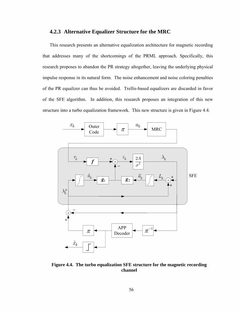
4.2.3 Alternative Equalizer Structure for the MRC
This research presents an alternative equalization architecture for magnetic recording
that addresses many of the shortcomings of the PRML approach. Specifically, this
research proposes to abandon the PR strategy altogether, leaving the underlying physical
impulse response in its natural form. The noise enhancement and noise coloring penalties
of the PR equalizer can thus be avoided. Trellis-based equalizers are discarded in favor
of the SFE algorithm. In addition, this research proposes an integration of this new
structure into a turbo equalization framework. This new structure is given in Figure 4.4.
Figure 4.4. The turbo equalization SFE structure for the magnetic recording channel
pkλ
kλ
ka
kr kzf 2
2A
σ+
+_
2g1g ka+
+
+kL
+
π 1π −APPDecoder
+
OuterCode MRC
kakx π
_
kx
SFE
56

4.3 Simulations
In this section, results and analyses will be given on the merits of using a linear-
complexity equalization algorithm in place of the partial-response filter and trellis-based
channel detector for a turbo equalization system on the magnetic recording channel. The
results attained are quite promising for the SFE system and can prove to be beneficial for
advancement in the field of magnetic recording research. Comparison results are given in
terms of BER performance; however, these error-rate versus SNR curves do not illustrate
the entire differences between the two systems. Complexity is an important issue that is
included in this discussion by means of figures showing complexity versus required SNR
given a set error-rate.
Simulations have been performed where the encoder is either a turbo code or an
LDPC code. When used in conjunction with either turbo codes or LDPC codes, the SFE
system can give up to 20% increase to the areal density of the magnetic recording media
given the same 10-5 BER requirement and SNR as the PR4-based system. When
incorporating the complexity factor in the performance results, the SFE system requires
up to 2 dB less than the PR4-based system if the BER requirement and complexity are
kept constant.
4.3.1 System Model Comparisons
The two main systems that are compared in this section will be referred to as the SFE
system and the partial-response system. Both of these systems employ turbo equalization
with ECC that must have a decoder capable of using soft inputs and providing soft
outputs. The only differences between these two systems are the partial-response
57

equalization filter and the algorithm used in the channel detector. In the partial-response
system, it has the additional filter to shorten the channel impulse response seen by the
detector; the channel detector for this system model can employ high-complexity
methods such as the BCJR algorithm or SOVA. The SFE system, depicted in Figure 4.4,
does not have this partial-response equalization filter, and thus the channel impulse
response appears longer for this channel detector.
4.3.2 Turbo Code Results
A Lorentzian channel with AWGN is considered. The data is protected by a rate-8/9
parallel-concatenated convolutional code with generator polynomial (23,31) with a sector
length of 4096, and it is decoded using the BCJR algorithm. The system structure
implements a turbo equalization scheme. The SNR that is referred to in this section is
defined as where is the amount of energy in an isolated transition pulse as
defined in section
/iE N iEo
2.2.
Performance comparisons have been completed between the SFE system and the
partial-response system. In the case of the partial-response system, the channel is
equalized to a PR target; both the PR4 and EPR4 targets are looked at. The channel
detector utilizes the BCJR algorithm in the PR-system.
The first set of results is BER performance curves given in Figure 4.5 for these
systems with channel density 3.0. Five turbo equalization iterations are assumed. The
SFE system outperformed the partial-response system for both targets in this simulation
setup. At this high density, the EPR4 target outperforms the PR4 target, but the SFE
turbo equalized system still outperforms the EPR4 turbo equalized system by more than
2.0 dB.
58

Figure 4.5. BER performance comparison of the PR system and SFE system with a rate-8/9 (23,31) turbo code, cD =3.0
The plot in Figure 4.6 compares the performance of the two systems as the value of
varies. Each point represents the required SNR to attain a BER of 10-5 at that
particular density value. These results show that for a system operating at around
= 10.25 dB and requiring the performance to be at BER=10-5, the SFE system
will provide approximately 12.5% more space for data on a hard disk drive than the
system using partial-response equalization. Moreover, not only will the SFE system
provide a larger hard disk drive given the same system parameters of a partial-response
turbo-equalized system with a turbo code, but it attains this gain without increasing the
complexity.
cD
0/iE N
While these results are interesting and quite promising for the SFE system, the rest of
this research work does not focus on this setup with a turbo code. As mentioned
previously, current turbo codes have a noise floor well above the target BER that is
59

Figure 4.6. Comparison of the PR system and SFE system with a rate-8/9 (23,31) turbo code with fixed BER=10-5 over a range of cD
desired for the magnetic recording industry. In addition, turbo decoders require a much
higher complexity and thus higher power requirements than what the industry wants to
tolerate. For these reasons, the remainder of the work will operate with LDPC codes in
its place.
4.3.3 LDPC Results
When working with the message-passing algorithm for LDPC decoding [35], one
variable to set for this algorithm is the maximum number of inner iterations allowed for
the decoder. The activity of setting the number of inner iterations for the APP ECC
decoder per outer turbo equalization iteration is referred to as scheduling. Often for a
turbo code used in turbo equalization, the scheduling sets the decoder at one inner
iteration per outer turbo equalization iteration. However, with LDPC decoders, it is more
common to set the inner iterations for the decoder to be higher than one [47]. For the
60
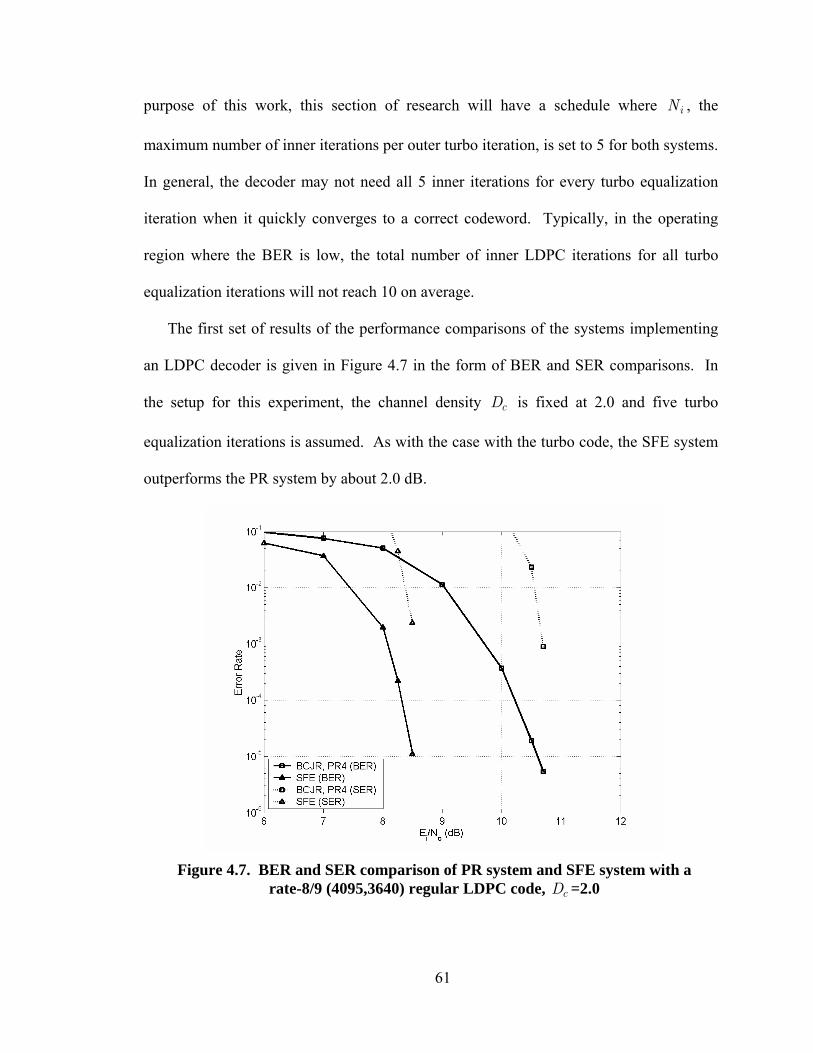
purpose of this work, this section of research will have a schedule where , the
maximum number of inner iterations per outer turbo iteration, is set to 5 for both systems.
In general, the decoder may not need all 5 inner iterations for every turbo equalization
iteration when it quickly converges to a correct codeword. Typically, in the operating
region where the BER is low, the total number of inner LDPC iterations for all turbo
equalization iterations will not reach 10 on average.
iN
The first set of results of the performance comparisons of the systems implementing
an LDPC decoder is given in Figure 4.7 in the form of BER and SER comparisons. In
the setup for this experiment, the channel density is fixed at 2.0 and five turbo
equalization iterations is assumed. As with the case with the turbo code, the SFE system
cD
outperforms the PR system by about 2.0 dB.
Figure 4.7. BER and SER comparison of PR system and SFE system with a rate-8/9 (4095,3640) regular LDPC code, cD =2.0
61

The data in Figure 4.8 compares the performance of these systems as the value of
var
same BER performance.
c
Figure 4.8. Comparison of PR system and SFE system with a rate-8/9 (4095,3640) regular LDPC code with fixed BER=10-5 over a range of cD
cD
ies. Each point represents the required SNR to attain a BER of 10-5 at that particular
density value. These results show that at 14 dB, the SFE can operate on a channel with
about a 20% higher density than the EPR4-equalized channel while still providing the
The figures given so far do show the performance gains of the SFE turbo equalized
system over using partial-response; however, those figures do not demonstrate the
omplexity costs of these systems. To this aim, Figure 4.9 plots the complexity versus
the amount of SNR required to attain a BER of 10-5 at channel density 2.5. Each curve
has five points, one for each of five iterations of the turbo equalizer. Here it can be seen
that the SFE has a gain of about 2 dB over the PR4-equalized channel without a large
62

Turbo equalization iteration
Figure 4.9. Complexity-performance comparison of the SFE system and the PR4-equalized system with a rate-8/9 (4095,3640) regular LDPC code
with fixed BER=10-5 at channel density 2.5
difference in complexity. In this plot, complexity is defined as operations per
information bit, where an operation is a multiply or an addition. However, since most of
the complexity for the SFE system is used in its filtering process, most of the operations
for the SFE method can be efficiently computed with one-clock-cycle multiply-
accumulate (MAC) operations in DSP processors rather than straight-forward multiplies
and adds. In MAC operations, the multiplies are computed at the same time as the adds,
thus some operations may seem hidden from an execution time perspective. In [48], one
MAC operation was implemented as efficiently as an instruction in a RISC CPU
architecture. Because an SFE architecture may gain more benefits of using MAC
operations than a trellis-based architectures can, the SFE may require less actual power
and operations than a BCJR system may.
63

4.3.4 Comparison with NPML
State-of-the-art detectors in industry are implementing NPML. For this reason, this
sec FE in magnetic recording in comparison to
NP
of the SFE
is t
me
4.3.5 Results
This research has proposed to forgo the use of partial-response equalization to a
method such as the SFE that does not enhance the noise and can outperform PRML as an
iter
tion looks at the performance of the S
ML. NPML has an inherent hard-output nature, and so it is often paired with a Reed-
Solomon code [49]. This hard-output precludes any use of turbo equalization.
A Lorentzian channel with AWGN is considered. The data is protected by a Reed-
Solomon (255,239,17) code with 8-bit symbols. For this setup, the soft output
ransformed into hard decisions for the Reed-Solomon (RS) decoder. Figure 4.10
demonstrates the BER performance of the NPML algorithm with the length of the
predictor filter, Lm , set at 4 against the SFE system, which uses no partial-response
equalization, at channel density 2.0. In these results, it is interesting to see that the SFE
has nearly the sa BER performance as the NPML algorithm for this setup, especially
given that the RS code is not exploiting any soft information that the SFE can provide.
ative detector. In fact, the SFE algorithm can provide up to 20% more capacity than
partial-response equalized detectors while maintaining low complexity costs. From these
results, it can be seen that the use of a linear-complexity algorithm is a promising
alternative to partial-response for magnetic recording.
64

Figure 4.10. BER Performance Comparison for data with RS (255,239,17) code at channel density 2.0
65

CHAPTER 5 NOVEL SFE CALCULATIONS FOR THE MRC
5.1 Introduction
Areal density in magnetic recording has been increasing faster than Moore’s Law, in
which the number of transistors per square inch on integrated circuits has doubled about
every year [1]. This increased storage capacity trend is likely to continue into the near
future. These increases come from enhanced performance in all areas of the recording
process. As it becomes more difficult to increase densities through improvements in the
media and heads, more consideration is given to advancements with signal processing
[50]. To this end, the use of iterative detectors for the magnetic recording channel was
introduced in [51]. Although these offer large performance gains over the conventional
PRML systems, they have not been adopted for commercial use, possibly because of the
performance versus complex tradeoff costs [50]. Power dissipation in hard disk drives is
a large concern because of the problems faced by electrical costs, system cooling, system
design, and reliability [17]. With these problems, the industry is challenged to find the
optimal algorithm and system architecture that provides high performance with
acceptable power requirements.
For this goal of finding a system architecture that allows for superior performance
with reasonable complexity costs, this research looks to the iterative SFE detector. In the
66

previous chapter, recall that this system has an improved performance curve over the
conventional PR-equalized system in a turbo equalization framework and has comparable
complexity. The complexity that was computed counted the instructions for the filtering
processes as adds and multiplies operations, and not as more efficient MAC operations.
With advances in low-power DSP chips and parallel processing, the SFE system becomes
a viable candidate for real application to the magnetic recording channel.
After scaling down the computation costs of the filtering processes by taking
advantage of the repetitive operations, a fixed overhead cost associated with the SFE
filter calculations becomes apparent. It is this overhead that the research in this chapter is
concerned with. To this aim, this chapter will discuss the development of a novel, lower
complexity method in determining updated SFE coefficients. Channel detectors
operating on the MRC are in an advantageous situation by the fact that the entire channel
itself and all channel statistics are fully known at the receiver. Because of these reasons,
a large portion of the SFE algorithm can be performed offline and stored, thus reducing
its complexity for this application even more. An obvious benefit of reduced complexity
is to allow for greater complexity in other parts of the system, perhaps in more turbo
equalization iterations thus increasing the system performance. It is also the hope of this
research that this work will lead to a practical iterative detector that will prove useful to
real applications in industry.
5.2 The computation of and eγ pγ
In Lopes’ original SFE algorithm [3], if the channel impulse response and channel
SNR is known, and respectively, then the filters can be completely determined by 0h 2σ
67

the values and as demonstrated by equations (4.2)-(4.4)eγ pγ . This section is concerned
with lowering the computational costs of finding these two values, as they are a large part
of the SFE algorithm. A new method will be outlined that reduces complexity while it
also prevents any degradation in performance to a significant degree.
Since the SFE in this setting has the magnetic recording channel characteristics
available, a complexity reduction can be obtained in the initial iteration. Recall that
during the first turbo iteration, the a priori information is generally not known, and
therefore ; it is only the value of that must be calculated at this stage. During
this initial phase, the SFE iterates about 3 times between
eγ0pγ =
(4.2) and (4.8) to jointly
determine the filter f and the scalar value . Each of these internal iterations involves
a matrix inverse, which is a highly complex operation on the order of O( ), where N
is the filter length. As the ISI increases, generally the length of the filters should
increase; so for channels with large amounts of ISI, such as a high capacity channel, three
matrix inverses in the first turbo iteration may prove to be quite costly.
eγ
3N
A quick observation can remove the need for these three matrix inverses for the first
turbo iteration. With the assumption that the channel characteristics are fully known and
fixed, then the first turbo iteration of the SFE will always converge to the same value for
, and thus it will always find the same filter f 1f, which will be designated eγ . This
vector can be calculated offline and stored for use in all initial turbo equalization
iterations. Similarly, the vectors 1g 2g and may also be determined offline and stored.
This method replaces 3 O( ) operations with simply the storage of one vector. 3N
Now the attention is turned to look at acquiring complexity savings after the initial
turbo iteration. In these stages, it was suggested in [3] to use its SEM estimator to
68

determine the values of and . However, the SEM estimator requires many
operations per channel bit, and this research seeks a reduction in this overhead. To
calculate , which is at turbo iteration i , the SEM estimator requires 3
operations/bit to find and 4 operations/bit to find , and then it will compute
. To calculate , the value of at turbo iteration i , the SFE requires
3 operations/bit to find and 4 operations/bit to find , and then it will compute
. In all, this SEM estimator needs approximately 14 operations/bit
every turbo iteration, other than the initial iteration, to find these two values. After
several turbo equalization iterations, the necessary complexity in these calculations can
become costly.
eγ pγ
,e iγ eγ
2,v iσiA
2, 2 /e i i v iAγ = ,p iγ pγ,σ
,σ
2,p iσ,p iA
2, ,2 /p i p i p iAγ =
Complexity costs can be reduced by forgoing the SEM scalar channel estimator in the
computation of and replacing it with the original estimates given by the general SFE
in
,p iγ
(4.7). With an extensive performance review of the SFE on magnetic recording
channel with turbo equalization, it has been observed that the SFE usually does not suffer
significant amounts of performance loss by changing this step. By eliminating the one
SEM estimator, the algorithm now requires approximately two operations/bit every turbo
iteration rather than seven for the calculation of this value.
An interesting aspect about the value of is that if the system is operating at an
adequate SNR to provide a low BER, the calculated estimates of do not vary by a
large degree between sectors for any fixed iteration i . To demonstrate this trait, Figure
5.1 shows scatter plots of the values versus the values for turbo iterations two to
five for a system where the channel density is 2.0 and the SNR is 8.5 dB. The range for
eγ
,e iγ
,e iγ ,p iγ
69

Iteration 2 Iteration 3
Iteration 4 Iteration 5
Figure 5.1. Scatter plots of eγ versus pγ for turbo iterations 2 through 5, cD =2.0, SNR = 8.5 dB
,p iγ is large, and the mean value for does tend to increase as the number of turbo
iterations increase, which is expected. This is true for both methods of estimating the
value for . However, the range for is much more limited in comparison, and this
range tends to remain small even as the number of turbo iterations increase. This
phenomenon suggests that the value of tends to be strongly dominated by the channel
characteristics rather than by performance gain, which is the case for the large range of
,p iγ
pγ ,e iγ
eγ
70

values for . This leads to the assumption that it may be reasonable to forgo any
calculations for and simply use a fixed value with the possibility of only a small
performance loss.
pγ
eγ
In the interest of reducing complexity, the value for will remain a single fixed
quantity for all turbo equalization iterations. This step is taken in the assumption
that the SFE algorithm is sufficiently robust so that it would not be greatly affected by
small variations in . One method in determining this fixed value is to look at the mean
of . Figure 5.2 plots the average value of for each turbo iteration i for a range of
channel densities. The value of appears anomalous compared to the other iterations
and is perhaps too optimistic. For this reason, for a specific channel density and
SNR could be determined by
eγ
fixedeγ
eγ
eγ ,e iγ
,1eγ
fixedeγ
[ ,2
11
Pfixede
iE EP
γ=
]e iγ⎡ ⎤⎢ ⎥= ⎢ ⎥−⎣ ⎦
∑ (5.1)
where is the total number of turbo equalization iterations. However, it is simpler to
use the found from a few offline iterations between
P
(4.2) and (4.8),1eγ for the value
. In this method, no offline simulations are necessary to determine the mean SNR
of the extrinsic information as needed for the method in
fixedeγ
(5.1). It has been observed that
there is not a significant performance difference between these two approximation
methods for determining the fixed value for . eγ
The result of all of these observations on and have given complexity
reductions for the SFE. Three matrix inverses in the initial turbo iteration have been
replaced with a few offline calculations. The filter
eγ pγ
f is now only a function of the
71

i
Figure 5.2. Average ,e iγ across sectors for each turbo iteration i for varying channel densities at an SNR that gives BER=10-5 at the fifth turbo iteration
variable as the SFE will now be using the approximation . Finally, all SEM
calculations have been eliminated.
fixedeγpγ
5.3 The Matrix Inverse
In the previous section, it was demonstrated not only how to reduce the calculations
previously required for the and computations, but it furthermore established how
to circumvent three matrix inverses in the first turbo equalization iteration. However,
there still remains one large matrix inversion for every iteration starting with the second
turbo iteration. This section outlines a strategy to calculate the filter
eγ pγ
f without the need
for any matrix inversions as opposed to the original algorithm as evidenced in (4.2).
72
Recall that with the assumption that the values of and are set, the feed-forward
filter
0h 2σ
f is solely a function of and . A brute force method to avoid the matrix
inverse is to build a lookup table with pre-calculated values of
eγ pγ
f for a range of and
values. Unfortunately, this will lead to a substantial amount of storage required. The
size of this lookup table can be considerably decreased given the results of the previous
section in that the value for generally does not significantly vary between iterations or
between sectors for the magnetic recording channel. Given an initial channel setup, all
possible vectors for
eγ
pγ
eγ
f are determined by only a very limited range of values for .
Even with the use of , the brute force method may still be implausible because of
the large range for all the possible values. The following sections present methods
that may be more economical in terms of storage and computational tradeoff costs.
eγ
fixedeγ
pγ
5.3.1 Conjugate Gradient Method
A popular iterative method in solving linear matrix equations is the conjugate
gradient (CG) method [52]. This can be applied to solving for f from (4.2), but by a
less complex means than using a matrix inversion explicitly by Gaussian elimination.
With a few iterations, some complexity savings may be gained with the CG method, but
at a cost of approximating the resulting filter coefficients.
0=Bf hThe CG method utilizes the fact that solving is equivalent to minimizing
the function
01
( )2T TΩ = −f f Bf f h . (5.2)
73

2 21 2* * *
1 1 2 21 2E E
α ασ= − − +B HH H H H H 2IHere the matrix is defined as such for
convenience. Because 10
−=f B h0( )∇Ω = −f Bf h , the unique minimizer of is Ω .
Starting with 0f f ( )Ω f, an initial guess for , the estimate for the minimum of is
improved by iterative steps. The minimum is guaranteed to exist in general only if is
positive definite and symmetric. In searching for this minimum, residuals are used,
which are computed by . If the residual is nonzero, then there exists a
positive number such that
B
kq
0ˆ
k = −q h B kf
ˆ( )kˆ( )k kρΩ + < Ωf qρ f
k
. At each CG iteration, the estimates
are updated by a scalar multiple of the search direction vector as kpkρ
1ˆ ˆk k kρ−= +f f p . Iteration stops when the residual reaches zero, or if it reaches some
other stop criterion since attempting to attain zero residual is unrealistic [52]. Based on
the method presented in [53], the CG algorithm is demonstrated by the following
pseudocode:
0 0 0
0 0
1 1 1 1
1 1
1 1
1 1
1
0
0
1
( , )/( ,
ˆ ˆ
( , )/( , )
ˆ ˆ
k
k k k k k
k k k k
k k k k
k k k k k
k k k k
k
k
k k
gg
ρ
ρρ
− − − −
− −
− −
− −
−
== −=
≠= +
=
= += −
== +
=
while
end
q h Bfp q
q
q q p Bp
f f pq q Bp
q q q qp q p
f f
) (5.3)
74
where denotes a dot product. The CG algorithm requires only one O( ) matrix-
vector multiply per iteration. If only a few iterations are used to estimate the filter, then
this process will have a lower complex than the explicit method requiring an O( )
inverse.
2N(, )⋅ ⋅
3N
0f One free parameter that must be chosen prior to execution is the initial guess for .
One guess could perhaps be MFf , which is the MF in the traditional ISI canceller that the
SFE algorithm reduces to when [3]. However, when the actual value for is
small, this may not be an accurate guess and more CG iterations would be necessary. For
small values, a better guess may be
pγ → ∞ pγ
00,( fixedp c
inv γ γ=B )h 1f, which is the filter pγ from
the initial turbo iteration that is calculated offline.
The question now arises as to how many CG iterations should be allowed in this
method. The residuals are mutually orthogonal, thus there can be at most N iterations
until convergence. For the application in this research, full convergence is not required,
particularly since that may lead to a method that has an O( ) complexity just as in the
explicit matrix inverse, and thus no computational savings are acquired. However, it is
desired to have a close approximation of the feed-forward filter, so more than one
iteration may be necessary. It has been observed that about 3 CG iterations is generally
sufficient for the purposes of this research work, and this gives us a method with an
O( ) complexity.
3N
23N
To demonstrate the merit of the approximation, a few experiments were performed to
compare the estimated filter from the CG method to the original SFE filter with all the
full calculations. The results of these experiments are shown in Table 5.1. The SNR was
75

Table 5.1. Comparison results of the CG-method filter f to the original SFE filter f
Density SNR pγ Error, iter. 1 Error, iter. 2 Error, iter. 3 1.0 4.5 dB 0 2.17% 0.47% 0.14% 1.0 4.5 dB 10 0.04% ≈ 0 ≈ 0 2.5 11.5 dB 0 13.01% 4.49% 1.63% 2.5 11.5 dB 10 0.61% 0.02% ≈ 0
set to provide a BER of at least 10-5 using the original filter f . Two different channel
densities were surveyed, and at each density, a low value and a high value for was
investigated. For three iterations of the CG algorithm, the approximated filter is
compared to the original filter. The approximation error is calculated as
pγ
2
2error % 100 SFE CG
SFE
−= ⋅
f ff
. (5.4)
0fMFfThe filter was used for the initial guess for . As expected, the resulting error % is
higher in cases with the low value because of the poor initial guess. pγ
With the CG method, finding an approximated SFE feed-forward filter is a lower
complexity operation than the original explicit inverse. To find the filters 1g 2g and , the
original method in equations (4.3) and (4.4) can remain. While the CG method may be a
viable option, the next section outlines a method that requires less computation than the
CG algorithm.
5.3.2 Incomplete Basis Method
In the previous section, a method using the CG algorithm was implemented to
approximate the feed-forward filter of the SFE. This reduced the amount of overhead
76
required for the SFE. In this section, a new method utilizing basis functions will be
implemented, which will lead to an O( ) algorithm for finding the feed-forward filter. N
fIn this new method implemented in this research, the filter is determined with
basis functions instead of a matrix inverse and may be written as
. (5.5) 1 1 2 2 M Mν ν ν= + + +f φ φ φ
Here the basis functions are denoted by , , , and the basis
coefficients are composed of the . Let F be the set of all possible vectors for
mφ 1,...m M= M N≤
fmν
given a specific channel setup and the use of . is a subset of the vector space
; however, it generally does not compose a subspace of as it is not closed under
vector addition and scalar multiplication. In the context of vector spaces, the definition
of a basis is a set of linearly independent vectors that span a vector space. Consequently,
basis functions of cannot be discussed in the same manner as in vector space basis
sets. However, in general the term basis implies the ability to generate an object in an
appropriate manner. For the purposes here, the basis set for F will be defined as a set of
linearly independent vectors that can generate any vector in the subset F under vector
addition and scalar multiplication.
fixedeγ F
N N
F
fAn important question for this basis method for finding is how to determine the
basis functions and how many must there be. Revisiting the general CG algorithm, if the
search directions are linearly independent and kfkp solves the problem
0 1 ,..., min ( )
kspan∈ +Ω
f f p pf (5.6)
77

ffor , this leads to the conclusion that in (5.5)1,2,...k = may require up to basis
functions. The underlying principle for this is that the vector
N
Nf minimizes Ω over
and thus satisfies
N
0N =Bf h .
fIn place of using a full set of basis functions to precisely determine the filter , this
research advocates an incomplete basis set that employs only a small number of
functions. While it is reasonable to assume that without a complete basis set that there
will be an error between the original vector and the approximated vector, it has been
observed that a small error in the feed-forward filter does not significantly affect the SFE
performance. Using only a handful of functions in the basis set is analogous to
performing only a few steps of the CG algorithm. The initial guess for 0f from the CG
method can be the first entry into the basis set. However, in this case, the orthogonal
search directions are predetermined. This is a sensible method given that in magnetic
recording the vector subset F is known, stable, and can be determined offline.
The immediate task is to determine which functions should be placed in this
incomplete basis set while attempting to maintain a low error % between the original
vector f and the filters formed from this incomplete basis. It would stand to reason that
since the feed-forward filter f is solely a function of , one source to be considered for
these basis functions is the group of filters resulting from the extreme values of this
variable. As the number of turbo iteration increases, the value for increases from 0
to ∞ . With this information, two of the vectors to be placed in the incomplete basis set
can be derived from the extreme values for , namely
pγ
pγ
1f MFf and pγ . However, these
two vectors in general are not orthogonal to each other, so the former vector’s projection
78
onto the latter vector can be subtracted off. The orthonormal set of vectors for this
incomplete basis with these two functions can now be written as
11
1 2
1 12
1 1 2
( , )( , )
MF MF
MF MF
=
−=
−
fφff φ f φφf φ f φ
. (5.7)
The optimal values for the basis coefficients are simply the scalar projections of
the desired
mν
f onto each . These can be calculated as mφ
(5.8) 1
2 2
( , )
( , )
ν
ν
=
=
f φ
f φ1
2
However, this requires knowledge of the feed-forward filter, which is precisely the filter
that this method is trying to approximate. What can be done is that these basis
coefficients, which are ultimately functions of , can be calculated offline for a range of
and stored with a relatively small lookup table.
pγ
pγ
With the feed-forward filter determined in this manner, the calculations for the
feedback filters can be rearranged to require fewer multiplications. The feed-forward
filter is written as
. (5.9) 1 1 2( ) ( )p pν γ ν γ= +f φ φ
The feedback filters may now be reorganized as
( )1 *1 1 1 1 2 2
1
1 1* *1 1 1 2 1 2
1 1
E
E E
αν ν
α αν ν
= +
= +
g H φ φ
H φ H φ (5.10)
( )2 *2 2 1 1 2 2
2
2 2* *1 2 1 2 2 2
2 2
E
E E
αν ν
α αν ν
= +
= +
g H φ φ
H φ H φ . (5.11)
79

With this arrangement, each of the original O( ) matrix-vector multiplies are replaced
with a formulation that contains two matrix-vector multiplies, but these may now be
computed offline and the only real-time calculations necessary are the scalar
multiplications and vector additions which give this method an O( )
complexity.
2N
1 23 3(N N μ+ + )
To better illuminate this incomplete basis method for finding the SFE feed-forward
filter, Figure 5.3 shows the entire subset for a specific channel setup with the channel
density at 2.5 and SNR = 11.5 dB. The x-axis is the index number of the filter
coefficients, the y-axis is the value for , and the z-axis is the value of the filter
coefficient. At around = 20, the filter has converged to
F
pγ
MFfpγ , so this value serves as
the upper limit for the range of required in a lookup table. Using only the two basis
functions from
pγ
(5.7), the resulting lookup table found for the basis coefficients is
displayed as a plot in Figure 5.4.
fIn this method of determining the feed-forward filter with imperfect basis vectors,
the computational costs are greatly reduced by having the matrix inverse completely
removed from every turbo equalization iteration. This method is also less complex than
the CG method in the previous section. To demonstrate the merit of this approximation,
a few experiments were performed to compare the estimated filter from the incomplete
basis method to the original SFE filter. The results of these experiments are shown in
Table 5.2. The SNR was set to provide a BER of at least 10-5. Two different densities
were surveyed, and at each density, a low value and a high value for were
investigated. The approximation error is calculated as in equation
pγ
(5.4). Compare these
results to those obtained in Table 5.1 for the CG method. That method may require a few
80

O( ) iterations before the approximated filter attains a similarly low error as in this
incomplete basis method, which is simply O( ).
2N
N
It is possible that with a given channel setup, the error % in the filters encountered
with this method may be larger than desired. To compensate for this, extra basis
functions may be added to the incomplete basis set. It is best to choose a function that
Table 5.2. Comparison results of the incomplete basis method to the original SFE filter f
Density SNR pγ Error 1.0 4.5 0 0 1.0 4.5 10 0.02% 2.5 11.5 0 0 2.5 11.5 10 0.29%
Coe
ffici
ent V
alue
Coefficient Index of Filter f
pγ
Figure 5.3. 3-D plot of all possible feed-forward filters at the given channel setup with channel density 2.5 and SNR=11.5 dB
81

Figure 5.4. Basis coefficient values as pγ changes for channel density 2.5 and SNR=11.5 dB
pγ
1
2
νν
reduces the % error the most, so for this objective, should be the generated
from the value of that produces
3′φ F∈f
pγ
( )( )
0 1 1 2 2, 2
0, 2
| ( ) (max
|
fixedp e
pfixed
p e
p pinv
inv
γ γγ
γ γ
ν γ ν γ⎧ ⎫⎪ ⎪− −⎪ ⎪⎪ ⎪⎨ ⎬⎪ ⎪⎪ ⎪⎪ ⎪⎩ ⎭
B h φ φ
B h
)
22N N+
. (5.12)
The function is then determined from by subtracting off the projections of the
other basis functions and normalizing as seen in
3′φ3φ
(5.7). The basis coefficient ν is
calculated in the same manner as in
3
(5.8).
With the complexity reductions taken from this entire chapter, the overhead of the
SFE algorithm has fallen drastically. In the first turbo iteration, the overhead has
decreased from O(3 ) to essentially zero since the three SFE filters are found
offline and are stored vectors. For all subsequent iterations, the overhead has decreased
3
82

from O( ) to O( ). This new SFE method
can be summarize by the following pseudocode:
3 22 14N N+ + 1 23( ) 2N N N Lμ+ + + +L
Offline: calculate and store f , & used for the first
turbo iteration 1g 2g
calculate from fixedeγ (5.1)
determine and based on 1φ 2φ (5.7) generate the lookup tables for the as in (5.8) mν
First SFE turbo iteration: fload the stored value for , & 1g 2g
All subsequent turbo iterations: calculate from (4.7) pγ
fcalculate from (5.9) calculate the feedback filters from (5.10) and (5.11)
5.4 Results
The previous sections have given rise to a lower complexity SFE method on the
magnetic recording channel. Though the merits of these complexity savings must still be
demonstrated in their BER performance capabilities compared to the original SFE
method. Results will be given in this section to highlight this aspect.
A Lorentzian channel with AWGN is considered. The data is protected by a rate-8/9
(4095,3640) regular LDPC code with column weight 3, and it is decoded using message
passing and turbo equalization. Figure 5.5 plots the BER and SER performance curves
for the original SFE system and the SFE with basis functions at channel density 2.0,
where channel density is in terms of . Using the basis functions for filter
approximations, the new system incurs a 0.03 dB performance loss.
50 / cPW T
83

Figure 5.5. BER and SER performance curves for the original SFE and the SFE with basis functions at cD =2.0
In Figure 5.6, the filter calculation overhead complexity versus required SNR to
achieve BER=10-5 is plotted between the original SFE and the SFE implementing the
basis functions at channel density 2.0. Each curve has five points, one for each of five
iterations of the turbo equalizer. The overhead costs counted in this graph are the
required filter calculations that are necessary before any of the equalizer’s filtering
processes can begin. This overhead lag needs to be kept at a minimum as it is a factor in
runtime, silicon, and power requirements. With this novel method of implementing an
imperfect basis set for filter approximations, the overhead complexity has been
drastically reduced with only a minor performance penalty. These results should help
open the door to that practical, iterative detector being sought in magnetic recording.
84

Figure 5.6. Overhead complexity versus performance comparison of the original SFE system and the SFE with basis functions at cD =2.0
85
CHAPTER 6 CONCLUSIONS
6.1 Summary of the Contributions
This dissertation has discussed the derivation, development, and evaluation of novel
turbo equalization techniques that address the colored noise problem on the magnetic
recording channel. One contribution presented is the NP-BCJR, a soft-output detection
strategy that mitigates colored noise in partial-response equalized channels. This
algorithm can be viewed as a combination of the traditional BCJR algorithm with the
notion of survivors and noise prediction. The NP-BCJR is a sub-optimal APP method to
combat noise correlation without the need for extending the trellis size. It also has an
added advantage over current-generation NPML, which has an inherent hard-output
nature, which precludes the possibility of soft error-control decoding as well as any form
of turbo equalization; conversely, NP-BCJR is readily applicable to SISO purposes and
iterative receivers. Owing to the complexity savings it offers, the NP-BCJR algorithm is
an attractive alternative to BCJR algorithms that extend the trellis size. Compared to the
classic BCJR algorithm ignoring the noise correlation, the NP-BCJR has shown to have a
marked improvement with minimal additional complexity.
86

Another major contribution of this dissertation work is the presentation of an
alternative equalization architecture for magnetic recording that addresses the
shortcomings of the PRML approach, which dominates magnetic recording. Specifically,
trellis-based equalizers are abandoned, leaving the underlying physical impulse response
in its natural form. These trellis-based equalizers are replaced by simpler equalization
strategies based on nonlinear filters whose complexity grows only linearly in their length.
For this aim, this research has focused on the linear-complexity SFE. In fact, it has been
shown that the SFE algorithm can provide up to 20% more capacity than EPR4-equalized
detectors while maintaining low complexity costs and maintaining a 10-5 BER
performance. From these results, it can be seen that the use of a linear-complexity
algorithm is a promising alternative to partial-response for magnetic recording and may
help push densities and hard disk drive capacities higher.
This work has also shown how to reduce the SFE complexity specifically for a fixed
and stable channel, such as in magnetic recording. The original Lopes SFE had a certain
amount of overhead cost in determining its filter coefficients. This overhead lag needs to
be kept at a minimum as it is a factor in runtime, silicon, and power requirements. The
research in this dissertation presented a novel method of implementing an imperfect basis
set for the filter approximations. With this novel method, the overhead complexity has
been drastically reduced with only a minor performance penalty. The original Lopes SFE
required approximately O( ) and O( ) computations for the first and subsequent
turbo iterations respectively. In contrast, implementing the new method requires only 0
and O( ) computations respectively.
3N 2N
N
87

The results of this work indicate that with using the new SFE method, it is possible to
increase the information density on magnetic media without raising the complexity
compared to trellis-based detectors. The most important result of the research is the
demonstration that partial-response equalization needs to be reconsidered because of the
amount of noise enhancement problems it adds to the overall system, especially since it
has been shown that the SFE system architecture outperforms the partial-response
equalized system. These results are important for practical application in the magnetic
recording industry, which is seeking a practical, iterative detector and pushing towards a
1 Tb/cm2 information storage goal.
6.2 Proposed Future Work
The channel model used throughout this research was based on longitudinal
recording. Yet, there is also another type of media magnetization known as
perpendicular recording, which has become important to the recording industry as it
expected to facilitate higher recording densities and thus progress in overall data storage
capacity. Since the growth in areal density for longitudinal recording is expected to lose
pace as the superparamagnetic limit is approached, research has begun focusing on the
perpendicular recording model.
The ultimate goal of this dissertation is to lead to a fully realized novel architecture
that will be found in a final product in a user’s personal computer. So for the continued
work for the practical application of this research for industry, many aspects of the read
head’s digital and analog electronics must be considered. One assumption made in this
research was that there is perfect timing recovery. The question remains open on how
88

robust the given algorithms are toward timing jitter problems. Exploring this issue may
lead to new algorithms to work conjunctively with the SFE filters to mitigate any timing
problems.
Another practical aspect of this future work is to extend the channel model to include
nonlinear noise effects. Sources of this noise include position jitter, width variation,
transition noise, and electronics noise. Studying these effects on the performance of the
proposed system should result in an even more realistic detector that would be of interest
to the recording industry.
In previous chapters, complexity is an issue that has been brought up a number of
times. Complexity was spoken in terms of the number of required adds and multiplies.
Yet not all operations are equivalent since the adds and multiplies in a MAC operation
are more efficiently computed than those done in an arithmetic logic unit. Complexity of
operations in different modules of a processor are not comparable because of differing
amounts of silicon required for the modules, various power requirements, and a different
amount of required clock cycles to complete the operation. Complexity is a very serious
issue in computing; and for this end, silicon and power requirement comparisons should
be certainly addressed.
89

REFERENCES [1] J. Moon, H. Thapar, B.V.K.V. Kumar, and K.A.S. Immink, “Signal
Processing for High Density Storage Channels,” IEEE Journal on Selected Areas in Communication, vol. 19, no. 4, pp. 577-581, April 2001.
[2] G.D. Fisher, W.L. Abbott, J.L. Sonntag, and R. Nesin, “PRML Detection
Boosts Hard-Disk Dive Capacity,” IEEE Spectrum, vol. 33, no. 11, pp. 70-76, Nov. 1996.
[3] R.R. Lopes, “Iterative Estimation, Equalization, and Decoding,” Ph.D.
Thesis, Georgia Institute of Technology, 2003. [4] R.R. Lopes and J.R. Barry, “Soft-Output Decision-Feedback Equalization
with a Priori Information,” IEEE Global Telecommunications Conference, vol. 3, pp. 1705-1709, San Francisco, CA, December 2003.
[5] N. Wei, M. Motani, and H.K. Garg, “Computation of Channel APP for
Magnetic Recording Channels with Colored Noise,” IEEE International Conference on Communication Systems, vol. 2, no. 25-28, pp. 769-773, Singapore, November 2002.
[6] A. Kavcic, “Soft-Output Detector for Channels with Intersymbol Interference and Markov Noise Memory,” IEEE Global Telecommunications Conference, pp. 728-732, Rio de Janeiro, Brazil, December 1999.
[7] J. Moon and J. Park, “Pattern-Dependent Noise Prediction in
Signal-Dependent Noise,” IEEE Journal on Selected Areas in Communication, vol. 19, no. 4, pp. 730-743, April 2001.
[8] J. Bergmans, “Discrete-Time Models for Digital Magnetic Recording,”
Philips Journal of Research, vol. 41, pp. 531-558, 1986. [9] P.H. Siegel and J.K. Wolf, “Modulation and Coding for Information
Storage,” IEEE Communications Magazine, vol. 29, no. 12, pp. 68-86, December 1991.
90

[10] F. Jorgensen, The Complete Handbook of Magnetic Recording,
McGraw-Hill, New York, NY, 1996. [11] J.G.D. Forney, “Maximum-Likelihood Sequence Estimation of Digital
Sequences in the Presence of Intersymbol Interference,” IEEE Transactions on Information Theory, vol. 18, May 1972.
[12] H. Kobayashi and D. Tang, “Application of Partial-response Channel
Coding to Magnetic Recording Systems,” IBM Journal of Research and Development, pp. 368-375, July 1970.
[13] H.K. Thapar and A.M. Patel, “A Class of Partial Response Systems for
Increasing Storage Density in Magnetic Recording,” IEEE Transactions on Magnetics, pp. 3666-3678, September 1987.
[14] T. Conway, “A New Target Response with Parity Coding for High
Density Magnetic Recording Channels,” IEEE Transactions on Magnetics, vol. 34, no. 4, pp. 2382-2386, July 1998.
[15] J. Fitzpatrick, J.K. Wolf, and L. Barbosa, “New Equalizer Targets for
Sampled Magnetic Recording Systems,” Twenty-fifth Asilomar Conference on Signals, Systems and Computers, vol. 1, pp. 30-34, Pacific Grove, CA, November 1991.
[16] W.E. Ryan, “A Study of Class I Partial Response Signaling for Magnetic
Recording,” IEEE Transactions on Magnetics, vol. 33, no.6, pp. 4543-4550, November 1997.
[17] S. Gurumurthi, A. Sivasubramaniam, M. Kandemir, and H. Franke,
“Reducing Disk Power Consumption in Servers with DRPM,” IEEE Computer Magazine, vol. 36, no. 12, pp. 59-66, December 2003.
[18] L.R. Bahl, J. Cocke, F. Jelinek, and R. Raviv, “Optimal Decoding of
Linear Codes for Minimal Symbol Error Rate,” IEEE Transactions on Information Theory, vol. 20, pp. 284-287, March 1974.
[19] D.J. Costello, Jr., A. Banerjee, C. He, and P.C. Massey, “A Comparison of
Low Complexity Turbo-like Codes,” Twenty-fifth Asilomar Conference on Signals, Systems and Computers, vol. 1, pp. 16-20, Pacific Grove, CA, November 2002.
[20] P. Robertson, P. Hoeher, and E. Villebrun, “Optimal and Sub-Optimal
Maximum A Posteriori Algorithms Suitable for Turbo Decoding,” European Transactions on Telecommunications, vol.8, no.2, pp. 119-125, March-April 1997.
91

[21] W.E. Ryan, L.L. McPheters, and S.W. McLaughlin, “Combined Turbo
Coding and Turbo Equalization for PR4-Equalized Lorentzian Channels,” Proceedings of the 38th Annual Conference on Information Sciences and Systems, pp. 489-494, Princeton, NJ, May 1998.
[22] W.E. Ryan, “Optimal Code Rates for Concatenated Codes on a PR4-
Equalized Magnetic Recording Channel,” IEEE Transactions on Magnetics, vol. 36, no.6, pp. 4044-4049, November 2000.
[23] P.R. Chevillat, E. Eleftheriou, and D. Maiwald, “Noise-Predictive Partial-
Response Equalizers and Applications,” IEEE International Conference on Communications, pp. 942-947, Chicago, IL, June 1992.
[24] E. Eleftherious and W. Hirt, “Noise-Predictive Maximum Likelihood
(NPML) Detection for the Magnetic Recording Channel,” IEEE International Conference on Communications, pp. 556-560, Dallas, TX, June 1996.
[25] J.D. Coker, E. Eleftheriou, R.L. Galbraith, and W. Hirt, “Noise-Predictive
Maximum Likelihood (NPML) Detection,” IEEE Transactions on Magnetics, vol. 34, no. 1, pp. 110-117, January 1998.
[26] A.J. Viterbi, “Error Bounds for Convolutional Codes and an
Asymptotically Optimum Decoding Algorithm,” IEEE Transactions on Information Theory, vol. IT-13, pp. 260-269, April 1967.
[27] T. Souvignier, M. Öberg, P.H. Siegel, R.E. Swanson, and J.K. Wolf,
“Turbo Decoding for Partial Response Channels,” IEEE Transactions on Communications, vol. 48, no. 8, pp. 1297-1308, August 2000.
[28] M.C. Reed and C.B. Schlegel, “An Iterative Receiver for the Partial
Response Channel,” IEEE International Symposium on Information Theory, p. 63, Cambridge, MA, August 1998.
[29] C. Douillard, M. Jézéquel, and C. Berrou, “Iterative Correction of
Intersymbol-Interference: Turbo-Equalization,” European Transactions on Telecommunications, vol. 6, no. 5, pp. 507-511, September-October 1995.
[30] J.G. Proakis, Digital Communications, McGraw-Hill, 3rd Edition, New
York, NY, 1995. [31] V. Franz and J.B. Anderson, “Concatenated Decoding with a
Reduced-Search BCJR Algorithm,” IEEE Journal on Selected Areas in Communication, vol. 16, no. 2, pp. 186-195, February 1998.
92

[32] J. Hagenauer and P. Hoeher, “A Viterbi Algorithm with Soft-Decision Outputs and its Applications,” IEEE Global Telecommunications Conference, vol. 3, pp. 1680-1686, Dallas, TX, November 1989.
[33] A. Roumy, I. Fijalkow, and D. Pirez, “Joint Equalization and Decoding:
Why Choose the Iterative Solution?” IEEE Vehicular Technology Conference, pp. 2989-2993, Amsterdam, Netherlands, September 1999.
[34] K.R. Narayanan, U. Dasgupta, and B. Lu, “Low Complexity Turbo
Equalization with Binary Precoding,” IEEE International Conference on Communications, pp. 1-5, New Orleans, LA, June 2000.
[35] R.C. Gallagher, Low-Density Parity-Check Codes, MIT Press, Cambridge,
MA, 1963. [36] D.J.C. MacKay and R. Neal, “Near Shannon Limit Performance of Low
Density Parity Check Codes,” IEE Electronics Letters, vol. 33, issue 6, pp. 457-458, March 1997.
[37] T. Souvignier and J.K. Wolf, “Turbo Decoding for Partial Response
Channels with Colored Noise,” IEEE Transactions on Magnetics, vol. 35, no. 5, September 1999.
[38] J. Bergmans, “Partial Response Equalization,” Philips Journal of
Research, vol. 42, no. 2, pp. 209-245, 1987. [39] S.U.H. Qureshi, “Adaptive Equalization,” Proceedings of the IEEE,
vol. 73, no. 9, pp. 1349-1387, September 1985. [40] J.G. Kenney and R. Wood, “Multi-level Decision Feedback Equalization:
an Efficient Realization of FDTS/DF,” IEEE Transactions on Magnetics, vol. 31, no. 2, pp. 1115-1120, March 1995.
[41] V.Y. Krachkovsky, Y.X Lee, and B. Liu, “Error propagation evaluation
for MDFE detection,” IEEE Transactions on Magnetics, vol. 33, no. 5, pp. 2770-2772, Sept. 1997.
[42] A. Glavieux, C. Laot, and J. Labat, “Turbo Equalization Over a Frequency
Selective Channel,” International Symposium on Turbo Codes and Related Topics, pp. 96-102, Brest, France, September 1997.
[43] M. Tücher, R. Koetter, and A.C. Singer, “Turbo Equalization: Principle
and New Results,” IEEE Transactions on Communications, vol. 50, no. 5, pp. 754-767, May 2002.
93

[44] D. Raphaeli and A. Saguy, “Reduced Complexity APP for Turbo Equalization,” IEEE International Conference on Communications, vol. 3, pp. 1940-1943, New York, NY, April-May 2002.
[45] A. Dejonghe and L. Vanderdorpe, “Turbo Equalization for Multilevel
Modulation: an Efficient Low-Complexity Scheme,” IEEE International Conference on Communications, vol. 3, pp. 1863-1867, New York, NY, April-May 2002.
[46] J. Rößler, W. Gerstacker, A. Lampe, and J. Huber, “Matched-Filter and
MMSE-Based Iterative Equalization with Soft Feedback for QPSK Transmission,” International Zurich Seminar on Broadband Communications, pp. 19-1 - 19-6, Zurich, Switzerland, February 2002.
[47] A. Thangaraj and S.W. McLaughlin, “Thresholds and Scheduling for
LDPC-Coded Partial Response Channels,” IEEE Transactions on Magnetics, vol. 38, no. 5, pp. 2307-2309, September 2002.
[48] P.F. Stelling and V.G. Oklobdzija, “Implementing Multiply-Accumulate
Operation in Multiplication Time,” Proceedings of the Thirteenth IEEE Symposium on Computer Arithmetic, pp. 99-106, Asilomar, CA, July 1997.
[49] I.S. Reed and G. Solomon, “Polynomial Codes over Certain Finite Fields,”
SIAM Journal on Applied Mathematics, vol. 8, pp. 300-304, 1960. [50] R. Lynch, E.M. Kurtas, A. Kuznetsov, E. Yeo, and B. Nikolić, “The
Search for a Practical Iterative Detector for Magnetic Recording,” IEEE Transactions on Magnetics, vol. 40, no. 1, pp. 213-218, January 2004.
[51] W.E. Ryan, “Performance of High Rate Turbo Codes on a PR4-Equalized
Magnetic Recording Channel,” IEEE International Conference on Communications, vol. 2, pp. 947-951, Atlanta, GA, June 1998.
[52] G.H. Golub and C.F. Van Loan, Matrix Computations, 3rd edition, The
John Hopkins University Press, Baltimore, MD, 1989. [53] M. Hestenes and E. Stiefel, “Methods of Conjugate Gradients for Solving
Linear Systems,” Journal of Research of the National Bureau of Standards 49, pp. 409-436, 1952.
94

VITA Elizabeth Chesnutt received the B.S. degree in Electrical Engineering Summa Cum
Laude from Auburn University in 1998. She received her M.S. and Ph.D. degrees in
Electrical and Computer Engineering in 1999 and 2005, respectively, from the Georgia
Institute of Technology majoring in telecommunications and digital signal
processing (DSP), and minoring in Mathematics.
Ms. Chesnutt’s previous experience involved applied research and development in
telecommunications, wireless system technologies, Synthetic Aperture Radar (SAR),
digital speech processing, passive optical networks, and wavelength division
multiplexing for fiber-optic cable.
During her graduate work, Ms. Chesnutt worked in the Communication Theory
Group under the advisement of Professor John R. Barry. Her current research focuses on
turbo equalization including linear-complexity algorithms, turbo codes, and LDPC codes.
Ms. Chesnutt is an active member of the Institute of Electrical and Electronics
Engineers (IEEE). She was honored in 1998 as IEEE’s student of the year for the state.
In 1999, she was awarded by Auburn University as their Outstanding Electrical
Engineering Student for the year.
95


![Multilevel-Coded QAM With MIMO Turbo-Equalization in ... · systems have to be more optimized toward packet-based transmission. The original suboptimal algorithms [2]–[4] for turbo-equalization](https://img.pdfslide.us/doc/110x75/5ecace6f261e3667c0215f45/multilevel-coded-qam-with-mimo-turbo-equalization-in-systems-have-to-be-more.jpg)


![LMMSE turbo equalization based on factor graphsliping/Research/Journal/53... · factor graphs, Gaussian message passing, linear MMSE. I. INTRODUCTION T URBO equalization [1]-[8] is](https://img.pdfslide.us/doc/110x75/6007243dfe2d385f6d5d46ad/lmmse-turbo-equalization-based-on-factor-lipingresearchjournal53-factor.jpg)
![Turbo equalization: principles and new results ...singer/pub_files/Turbo...Combined turbo codingand equalization [20],[21]includes threeor morelayers: two or more coding layers as](https://img.pdfslide.us/doc/110x75/600724985f3e7f70086519b2/turbo-equalization-principles-and-new-results-singerpubfilesturbo-combined.jpg)