Embed Size (px)
Citation preview
Novel Sensing and Inference Techniques in Air andWater Environments
by
Xiaochi Zhou
Department of Civil and Environmental EngineeringDuke University
Date:Approved:
John D. Albertson, Co-Supervisor
Marco Marani, Co-Supervisor
Sonia Silvestri
Gabriel G. Katul
Dissertation submitted in partial fulfillment of the requirements for the degree ofDoctor of Philosophy in the Department of Civil and Environmental Engineering
in the Graduate School of Duke University2015
Abstract
Novel Sensing and Inference Techniques in Air and Water
Environments
by
Xiaochi Zhou
Department of Civil and Environmental EngineeringDuke University
Date:Approved:
John D. Albertson, Co-Supervisor
Marco Marani, Co-Supervisor
Sonia Silvestri
Gabriel G. Katul
An abstract of a dissertation submitted in partial fulfillment of the requirements forthe degree of Doctor of Philosophy in the Department of Civil and Environmental
Engineeringin the Graduate School of Duke University
2015

Copyright c© 2015 by Xiaochi ZhouAll rights reserved except the rights granted by the
Creative Commons Attribution-Noncommercial Licence
Abstract
Environmental sensing is experiencing tremendous development due largely to the
advancement of sensor technology and wireless technology/internet that connects
them and enable data exchange. Environmental monitoring sensor systems range
from satellites that continuously monitor earth surface to miniature wearable de-
vices that track local environment and people’s activities. However, transforming
these data into knowledge of the underlying physical and/or chemical processes re-
mains a big challenge given the spatial, temporal scale, and heterogeneity of the
relevant natural phenomena. This research focuses on the development and applica-
tion of novel sensing and inference techniques in air and water environments. The
overall goal is to infer the state and dynamics of some key environmental variables
by building various models: either a sensor system or numerical simulations that
capture the physical processes.
This dissertation is divided into five chapters. Chapter 1 introduces the background
and motivation of this research. Chapter 2 focuses on the evaluation of different
models (physically-based versus empirical) and remote sensing data (multispectral
versus hyperspectral) for suspended sediment concentration (SSC) retrieval in shal-
low water environments. The study site is the Venice lagoon (Italy), where we
compare the estimated SSC from various models and datasets against in situ probe
measurements. The results showed that the physically-based model provides more
robust estimate of SSC compared against empirical models when evaluated using the
iv
cross-validation method (leave-one-out). Despite the finer spectral resolution and the
choice of optimal combinations of bands, the hyperspectral data is less reliable for
SSC retrieval comparing to multispectral data due to its limited amount of historical
dataset, information redundancy, and cross-band correlation.
Chapter 3 introduces a multipollutant sensor/sampler system that developed for use
on mobile applications including aerostats and unmanned aerial vehicles (UAVs).
The system is particularly applicable to open area sources such as forest fires, due
to its light weight (3.5 kg), compact size (6.75 L), and internal power supply. The
sensor system, termed Kolibri, consists of low-cost sensors measuring CO2 and CO,
and samplers for particulate matter and volatile organic compounds (VOCs). The
Kolibri is controlled by a microcontroller, which can record and transfer data in real
time using a radio module. Selection of the sensors was based on laboratory test-
ing for accuracy, response delay and recovery, cross-sensitivity, and precision. The
Kolibri was compared against rack-mounted continuous emission monitors (CEMs)
and another mobile sampling instrument (the “Flyer”) that had been used in over
ten open area pollutant sampling events. Our results showed that the time series of
CO, CO2, and PM2.5 concentrations measured by the Kolibri agreed well with those
from the CEMs and the Flyer. The VOC emission factors obtained using the Kolibri
are comparable to existing literature values. The Kolibri system can be applied to
various open area sampling challenging situations such as fires, lagoons, flares, and
landfills.
Chapter 4 evaluates the trade-off between sensor quality and quantity for fenceline
monitoring of fugitive emissions. This research is motivated by the new air quality
standard that requires continuous monitoring of hazardous air pollutants (HAPs)
along the fenceline of oil and gas refineries. Recently, the emergence of low-cost
sensors enables the implementation of spatially-dense sensor network that can po-
tentially compensate for the low quality of individual sensors. To quantify sensor
v
inaccuracy and uncertainty of describing gas concentration that is governed by tur-
bulent air flow, a Bayesian approach is applied to probabilistically infer the leak
source and strength. Our results show that a dense sensor network can partly com-
pensate for low-sensitivity or high noise of individual sensors. However, the fenceline
monitoring approach fails to make an accurate leak detection when sensor/wind bias
exists even with a dense sensor network.
Chapter 5 explores the feasibility of applying a mobile sensing approach to estimate
fugitive methane emissions in suburban and rural environments. We first compare
the mobile approach against a stationary method (OTM33A) proposed by the US
EPA using a series of controlled release tests. Analysis shows that the mobile sensing
approach can reduce estimation bias and uncertainty compared against the OTM33A
method. Then, we apply this mobile sensing approach to quantify fugitive emissions
from several ammonia fertilizer plants in rural areas. Significant methane emission
was identified from one plant while the other two shows relatively low emissions.
Sensitivity analysis of several model parameters shows that the error term in the
Bayesian inference is vital for the determination of model uncertainty while others
are less influential. Overall, this mobile sensing approach shows promising results for
future applications of quantifying fugitive methane emission in suburban and rural
environments.
vi

This work is dedicated to my parents Jianming Zhou, Mengxia Zhou, and my
wife Mandy Xu
vii
Contents
Abstract iv
List of Tables xi
List of Figures xii
Acknowledgements xvii
1 Introduction 1
2 Remote Sensing Retrieval of Suspended Sediment Concentration inShallow Coastal Waters 6
2.1 Introduction . . . . . . . . . . . . . . . . . . . . . . . . . . . . . . . . 6
2.2 Methods . . . . . . . . . . . . . . . . . . . . . . . . . . . . . . . . . . 9
2.2.1 Study site and datasets . . . . . . . . . . . . . . . . . . . . . . 9
2.2.2 Data processing . . . . . . . . . . . . . . . . . . . . . . . . . . 12
2.2.3 Radiative transfer model . . . . . . . . . . . . . . . . . . . . . 14
2.2.4 Empirical retrieval models . . . . . . . . . . . . . . . . . . . . 17
2.2.5 Calibration and validation . . . . . . . . . . . . . . . . . . . . 18
2.2.6 Band selection . . . . . . . . . . . . . . . . . . . . . . . . . . . 18
2.3 Results . . . . . . . . . . . . . . . . . . . . . . . . . . . . . . . . . . . 20
2.3.1 Atmospheric correction validation . . . . . . . . . . . . . . . . 20
2.3.2 Evaluation of bottom reflectance . . . . . . . . . . . . . . . . 23
2.3.3 SSC estimation using Hyperion data: model calibration andvalidation . . . . . . . . . . . . . . . . . . . . . . . . . . . . . 24
viii

2.3.4 SSC estimation using multi-spectral data . . . . . . . . . . . . 32
2.4 Conclusion and Discussion . . . . . . . . . . . . . . . . . . . . . . . . 35
3 Development and Evaluation of a Lightweight Sensor System forAerial Emission Sampling from Open Area Sources 39
3.1 Introduction . . . . . . . . . . . . . . . . . . . . . . . . . . . . . . . . 39
3.2 Method . . . . . . . . . . . . . . . . . . . . . . . . . . . . . . . . . . 42
3.3 Sensor performance evaluation . . . . . . . . . . . . . . . . . . . . . . 45
3.3.1 CO sensor performance . . . . . . . . . . . . . . . . . . . . . . 45
3.3.2 CO2 sensor performance . . . . . . . . . . . . . . . . . . . . . 47
3.3.3 Pump system performance . . . . . . . . . . . . . . . . . . . . 47
3.3.4 VOC sampling performance . . . . . . . . . . . . . . . . . . . 49
3.3.5 Evaluation of rotor wash on Kolibri sampling . . . . . . . . . 50
3.3.6 Open detonation experiment . . . . . . . . . . . . . . . . . . . 52
3.4 Conclusion . . . . . . . . . . . . . . . . . . . . . . . . . . . . . . . . . 54
4 Fenceline Monitoring: A Bayesian Approach to Locating FugitiveLeaks 55
4.1 Introduction . . . . . . . . . . . . . . . . . . . . . . . . . . . . . . . . 55
4.2 Method . . . . . . . . . . . . . . . . . . . . . . . . . . . . . . . . . . 58
4.2.1 Dispersion model and dispersion physics . . . . . . . . . . . . 60
4.2.2 Sensor model and sensor physics . . . . . . . . . . . . . . . . . 65
4.2.3 Bayesian inference model . . . . . . . . . . . . . . . . . . . . . 67
4.2.4 Simulation setup . . . . . . . . . . . . . . . . . . . . . . . . . 69
4.3 Results and discussion . . . . . . . . . . . . . . . . . . . . . . . . . . 71
4.3.1 Base condition . . . . . . . . . . . . . . . . . . . . . . . . . . 72
4.3.2 Sensor detection limits (sensitivity) on leak detection . . . . . 74
4.3.3 Wind direction on leak detection . . . . . . . . . . . . . . . . 75
ix
4.3.4 Sensor errors on leak detection . . . . . . . . . . . . . . . . . . 78
4.3.5 Wind measurement errors on leak detection . . . . . . . . . . 80
4.4 Conclusion . . . . . . . . . . . . . . . . . . . . . . . . . . . . . . . . . 82
5 A Mobile Sensing Approach for Operational Detection of FugitiveMethane Emissions 84
5.1 Introduction . . . . . . . . . . . . . . . . . . . . . . . . . . . . . . . . 84
5.2 Source inference from a mobile sensor . . . . . . . . . . . . . . . . . . 85
5.3 Source inference from a stationary sensor . . . . . . . . . . . . . . . . 89
5.4 Experiments . . . . . . . . . . . . . . . . . . . . . . . . . . . . . . . . 90
5.4.1 Controlled release experiment . . . . . . . . . . . . . . . . . . 90
5.4.2 Ammonia fertilizer plants sampling . . . . . . . . . . . . . . . 91
5.5 Results and discussion . . . . . . . . . . . . . . . . . . . . . . . . . . 92
5.5.1 Controlled release results . . . . . . . . . . . . . . . . . . . . . 92
5.5.2 Ammonia fertilizer plants sampling results . . . . . . . . . . . 96
5.6 Conclusion . . . . . . . . . . . . . . . . . . . . . . . . . . . . . . . . . 98
6 Conclusion 99
A Modified Gaussian plume model (Chapter 4) 103
Bibliography 105
Biography 115
x
List of Tables
2.1 Satellite data used in this study . . . . . . . . . . . . . . . . . . . . . 13
2.2 List of variables used in Eqn. 2.1 to 2.7 . . . . . . . . . . . . . . . . . 19
2.3 Least RMSE (FTU) with RTM from using model calibration and val-idation . . . . . . . . . . . . . . . . . . . . . . . . . . . . . . . . . . . 26
2.4 RMSE estimated using multispectral data . . . . . . . . . . . . . . . 32
3.1 Sensor package components . . . . . . . . . . . . . . . . . . . . . . . 44
3.2 Fan test experiment summary . . . . . . . . . . . . . . . . . . . . . . 51
4.1 Meteorological related variable . . . . . . . . . . . . . . . . . . . . . . 64
4.2 Computational simulation parameters . . . . . . . . . . . . . . . . . . 72
4.3 Model performance analysis . . . . . . . . . . . . . . . . . . . . . . . 72
xi
List of Figures
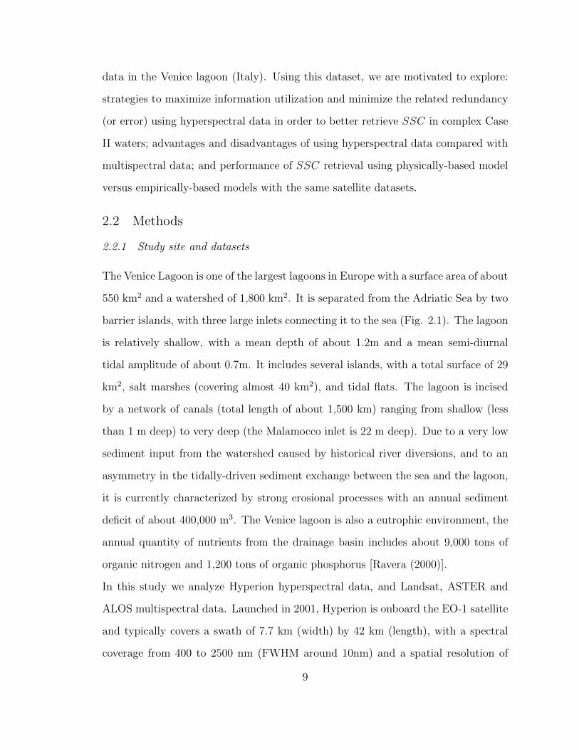
2.1 Map of the Venice lagoon showing the location of the 10 measurementstations (red circles, Ve1 to Ve10). The footprint of a typical Hyperionscene is shown as a red box. The Venice lagoon is shown as a whitebox in the Google Earth image of Italy. . . . . . . . . . . . . . . . . 10
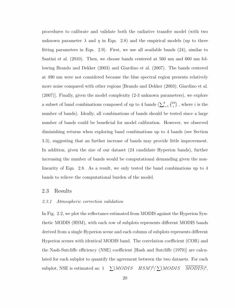
2.2 Comparison of reflectance estimated from MODIS against the Hype-rion Synthetic MODIS (HSM). Colors denote the density (in percent-age) of the points, which is estimated as a 2 dimensional histogramusing 20 equally spaced bins in both x and y directions. Yellow (black)means a large (low) density of points in a given area of the plot. Thecorrelation coefficient (COR) and the Nash-Sutcliffe efficiency coeffi-cient (NSE) are indicated in each subplot. . . . . . . . . . . . . . . . 21
2.3 Calibration of SSC using all Hyperion bands based on different bot-tom reflectance (βb). . . . . . . . . . . . . . . . . . . . . . . . . . . . 23
2.4 (a) RMSE of calibrated SSC as a function of absorption and backscat-tering coefficient using all 24 Hyperion bands, (b) estimated versusmeasured SSC using optimal γ and η in (a). . . . . . . . . . . . . . . 24
2.5 RMSE of the SSC calibration as a function of absorption and backscat-tering coefficient using bands centered at (a) 660 nm (7 spectral bandsfrom 630 nm to 690 nm), and (b) 560 nm (9 spectral bands rangingfrom 520 nm to 600 nm). . . . . . . . . . . . . . . . . . . . . . . . . . 25
2.6 Calibration and validation of the RTM using different number of bandscombinations. In the box-whisker plots, the red central line is themedian, the edges of the box are the 25th and 75th percentiles, thewhiskers extend to the extreme data points within approximately �2.7standard deviation from the mean (covering 99.3% data), and outliersare plotted as red crosses. Out of range data (indicate complete modelfailure) are represented with an arrow and the corresponding RMSEvalues are reported next to it. . . . . . . . . . . . . . . . . . . . . . . 27
xii
2.7 Calibration and validation of the radiative transfer model (RTM) us-ing different number of bands combinations: mean and standard devi-ation, which is represented as error bar (a and b), and minimum (c andd) of model output, computed at a band using all the possible pairsof that band with the others. Out of range data (indicate completemodel failure) are represented with an arrow and the correspondingRMSE values are reported next to it. . . . . . . . . . . . . . . . . . . 29
2.8 Calibration and validation of the relative transfer model (RTM) us-ing: single band (a and b); two bands with mean and one standarddeviation (error bar) (c and d) and minimum (e and f), computed ata band using all the possible pairs of that band with the other. Outof range data are represented with an arrow and values reported nextto it, bands fail with empirical models are marked as a black cross. . 30
2.9 Validation of RTM using different subset size of multispectral data(total of 52). In the box-whisker plots, the red central line is themedian, the edges of the box are the 25th and 75th percentiles, thewhiskers extend to the extreme data points within approximately �2.7standard deviation from the mean (covering 99.3% data), and outliersare plotted as red crosses. For comparison, the median, max, and minRMSE estimated using the Hyperion data (total of 20) with 2 bandsare also plotted. . . . . . . . . . . . . . . . . . . . . . . . . . . . . . . 33
2.10 Hyperion Synthetic ETM+ (HSE) reflectance plotted as a function ofturbidity along with the multispectral data. . . . . . . . . . . . . . . 34
3.1 Disassembled view of the Kolibri system . . . . . . . . . . . . . . . . 41
3.2 Lab testing of CO sensor: (a) sensor accuracy, and (b) sensor precision 45
3.3 Time series of CO measurement using California Analytical Instru-ments Model 200 (CAI-200), Horiba VIA-510 Gas Analyzer (HVIA-510), and the EC4-500 CO sensor, with two different burn materials:Kentucky Blue Grass stubble (KBGS) and wheat stubble (WS) . . . 46
3.4 Time series of CO2 measurement using LICOR 820 analyzer and theDX6220 CO2 sensor . . . . . . . . . . . . . . . . . . . . . . . . . . . . 47
3.5 Kolibri pump system evaluation: (a) the flow rate and the pressuresensor output relationship, where the errorbar is one standard devia-tion, and (b) 2.5 simultaneously sampled using the Kolibri pump andthe Leland Legacy pump during several burn facility tests . . . . . . 48
xiii
3.6 six selected VOC sampled from SUMMA canister (SC) versus Tenaxtube (TX) in OBTF . . . . . . . . . . . . . . . . . . . . . . . . . . . 49
3.7 Time series of calibrated PM2.5 concentration measured by DustTrakwith and without fan from OBTF . . . . . . . . . . . . . . . . . . . . 51
3.8 Above-ambient CO2 (green) and CO (red) concentration measured bythe Kolibri system during the 2nd detonation. . . . . . . . . . . . . . 52
3.9 Time series of CO (left axis) and CO2 (right axis) measurement during4 detonation experiments in Alaska, USA . . . . . . . . . . . . . . . . 53
4.1 The fenceline inference flowchart: x0 (xi) and Q0 (Qj) are the loca-tion and leak rate of the actual (hypothetical) fugitive leak(s), respec-tively. CDP
0 pxq|I0 is the above-ground concentration field caused bythe actual leak (x0, Q0) driven by actual meteorological and landscapeconditions (I0). CDM
i,j pxq|I is the modeled above-ground concentrationfield given a hypothetical leak scenario (xi, Qj) and estimated meteo-rological and landscape conditions (I). CSP
0 pxkq and CSMi,j pxkq are the
measured and modeled concentration signal reported by the kth sensor(located at xk) given concentration fields CDP
0 pxq|I0 and CDMi,j pxq|I,
respectively. δj,i is the difference between CSP0 pxkq and CSM
i,j pxkq. eDMand eSM represent the error introduced by the dispersion model andsensor characteristics, respectively. P pxi, Qjq is the estimated proba-bility of leak scenario (xi, Qj) from Bayesian inference given δi,j, e
DM ,and eSM . . . . . . . . . . . . . . . . . . . . . . . . . . . . . . . . . . . 59
4.2 5 years wind direction distribution in Philadelphia (top left), CorpusChristi (top middle), and using the stochastically wind direction func-tion. The 5-years averaged probability of covering wind direction from0 to 2π as function of time for different wind scenarios . . . . . . . . 63
4.3 A cartoon of the computational domain containing rectangular gridcells with a size of ∆x � ∆y. Each grid cell (e.g. xi) is treated as ahypothetical leak location with leak rate Qj, which is detonated byan open circle. The actual leak located at x0 with leak rate of Q0 isshown as a solid circle. Sensors (solid triangles) are evenly distributedalong each side of the fenceline with a length of L0 . . . . . . . . . . 69
4.4 Time series of normalized leak localization error (εxptq) and leak strengtherror (εQ) for point-scale real-time sensors (PS0), line-averaged real-time sensors (LS0), and point-scale time-integrated sensors at dailyresolution (TS1): wind direction from Philadelphia site . . . . . . . . 73
xiv

4.5 Time series of normalized leak localization error (εxptq) and leak strengtherror (εQ) for point-scale real-time sensors (PS0), line-averaged real-time sensors (LS0), and point-scale time-integrated sensors at dailyresolution (TS1): sensor quantity versus sensor lower detection limit(dL) with wind direction from Philadelphia site . . . . . . . . . . . . 75
4.6 Time series of normalized leak localization error (εxptq) and leak strengtherror (εQ) for point-scale real-time sensors (PS0), line-averaged real-time sensors (LS0), and point-scale time-integrated sensors at dailyresolution (TS1): wind direction from Corpus Christi (CC), Philadel-phia (Ph), and the stochastic wind direction model (ST ) . . . . . . . 76
4.7 Cumulative density function (CDF) of concentration measured overone year by PS0 (solid line) and LS0 (dash line) sensors located atdifferent sides of the fenceline with wind direction from Corpus Christi(CC), Philadelphia (Ph), and the stochastic wind direction model(ST ). Sensor lower detection limit (dL) is denoted by dash grey line . 77
4.8 Time series of normalized leak localization error (εxptq) and leak strengtherror (εQ) for point-scale real-time sensors (PS0), line-averaged real-time sensors (LS0), and point-scale time-integrated sensors at dailyresolution (TS1): sensor quantity versus sensor bias (Rs
µ) with winddirection from Philadelphia site . . . . . . . . . . . . . . . . . . . . . 78
4.9 Time series of normalized leak localization error (εxptq) and leak strengtherror (εQ) for point-scale real-time sensors (PS0), line-averaged real-time sensors (LS0), and point-scale time-integrated sensors at dailyresolution (TS1): sensor quantity versus sensor noise (Rs
σ) with winddirection from Philadelphia site . . . . . . . . . . . . . . . . . . . . . 79
4.10 Time series of normalized leak localization error (εxptq) and leak strengtherror (εQ) for point-scale real-time sensors (PS0), line-averaged real-time sensors (LS0), and point-scale time-integrated sensors at dailyresolution (TS1): sensor quantity versus wind angle bias (θeµ) withwind direction from Philadelphia site . . . . . . . . . . . . . . . . . . 80
4.11 Time series of normalized leak localization error (εxptq) and leak strengtherror (εQ) for point-scale real-time sensors (PS0), line-averaged real-time sensors (LS0), and point-scale time-integrated sensors at dailyresolution (TS1): sensor quantity versus wind angle noise (θeσ) withwind direction from Philadelphia site . . . . . . . . . . . . . . . . . . 81
5.1 A google earth image of the controlled release study site. Each pinrepresents a leak location . . . . . . . . . . . . . . . . . . . . . . . . . 90
xv

5.2 Dz estimated from model and data . . . . . . . . . . . . . . . . . . . 94
5.3 Estimated and metered methane leak from the blind experiments inthe controlled release experiments using stationary (OTM33A) andmobile sensing approach . . . . . . . . . . . . . . . . . . . . . . . . . 94
5.4 An example plume transect in Enid, OK, where the elevated red barindicates above ambient CH4 concentration . . . . . . . . . . . . . . . 95
5.5 pdf of the leak rate from ammonia plant located at Enid, OK . . . . 97
5.6 An example plume transect in Enid, OK, where the elevated red barindicates above ambient CH4 concentration . . . . . . . . . . . . . . . 97
xvi

Acknowledgements
First, I would like to express my gratitude to my co-advisors Dr. John Albertson
and Dr. Marco Marani for their continuous support and inspiration throughout my
Ph.D. study. I would like to thank Dr. Sonia Silverstri and Dr. Gaby Katul for
serving in my committee and providing their professional advice on remote sensing
analysis and micro-meteorology, respectively. This dissertation can not be finished
without the help from all my committee members.
I would also like to thank Dr. Brian Gullett at US EPA who offered me a student
service contractor opportunity under his supervision, and other colleagues at EPA:
Johanna Aurell, William Mitchell, Dennis Tabor, and Chris Pressley for their help
of design and test of the sensor system.
Many thanks to my fellow graduate students and friends at Duke and University of
Washington who gave invaluable support throughout my graduate school journey. In
particular, I would like to acknowledge Albertson’s group members: Tan Zi, Jun Yin,
Tiffany Wilson, and Tierney Harvey; Marani’s group members: Gabriele Manoli,
Meijing Zhang, Fateme Yousefi, Enrico Zorzetto, Yun Jian, and Yi Xiao; Katul’s
group members: Khaled Ghannam, Cheng-Wei Huang, and Tomer Duman.
Special thanks goes to Prof. Erkan Istanbulluoglu, who served as my advisor for my
MS degree and introduced me the fascinating field of Ecohydrology.
The travel of the ammonia plants was supported by Environmental Defense Fund.
The author also thanks the support from the Google Earth Outreach for help with
xvii

collecting measurements from public roads next to the ammonia plant. Part of this
work was done when the author was served as a student service contractor at the US
EPA, ORD. Any opinions, findings, and conclusions or recommendations expressed
in this material are those of the authors and do not necessarily reflect the views of
the Environmental Defense Fund or the Environmental Protection Agency.
xviii
1
Introduction
Environmental sensing is experiencing tremendous development due largely to the
advancement of sensor technology and the Internet and wireless technology that con-
nects distributed sensors together [Hart and Martinez (2006); Estrin et al. (2001)].
The scale of environmental monitoring sensors ranges from satellites that continu-
ously monitor earth surface to miniature, wearable devices that track local environ-
ment. Engineers predicted that sensors would eventually evolve to “smart dust”,
which are sensors as small as dust particles that can make real-time observation as
a network in a unprecedented spatial and temporal resolutions [Lohr (2010)]. How-
ever, transforming these data into our knowledge of the underlying physical/chemical
processes remains a big challenge given the spatial and temporal scale and hetero-
geneity of the relevant natural phenomena. New data can be used to quantify some
environmental variables that are not directly measured before and provide better
statistics for some variables given a larger sample size. However, excessive data will
create another degree of problem for validating environmental models, such as data
cross-correlation and redundancy. Meanwhile, the discrepancy of spatial and tem-
poral scales among dataset and between the data and the model may become even
1
worse. In the author’s point of view, the lack of data to constrain models speci-
fied by physically/chemically meaningful parameters will be eventually replaced by
the problem of choosing the appropriate dataset and incorporating sensor errors for
model evaluation.
This dissertation aims to develop and apply novel sensing and inference techniques
in a board spectrum of environmental problems, including development of sensor
system for open area emission sampling, remote sensing retrieval of suspended sed-
iment concentration in shallow water environments, evaluation of trade-off between
sensor quality and quantity for fenceline monitoring, and mobile sensing for identi-
fying fugitive methane emissions. The overall goal is to infer the state or dynamics
of some key environmental variables from measurements by building various models:
either a sensor system that can be used for field sampling or numerical simulations
based on the physical processes. The core part of the dissertation is organized by
topics of applications.
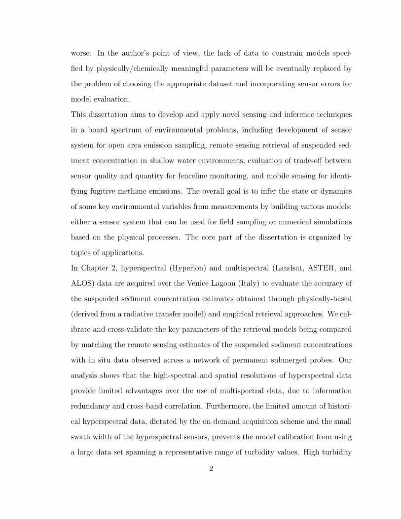
In Chapter 2, hyperspectral (Hyperion) and multispectral (Landsat, ASTER, and
ALOS) data are acquired over the Venice Lagoon (Italy) to evaluate the accuracy of
the suspended sediment concentration estimates obtained through physically-based
(derived from a radiative transfer model) and empirical retrieval approaches. We cal-
ibrate and cross-validate the key parameters of the retrieval models being compared
by matching the remote sensing estimates of the suspended sediment concentrations
with in situ data observed across a network of permanent submerged probes. Our
analysis shows that the high-spectral and spatial resolutions of hyperspectral data
provide limited advantages over the use of multispectral data, due to information
redundancy and cross-band correlation. Furthermore, the limited amount of histori-
cal hyperspectral data, dictated by the on-demand acquisition scheme and the small
swath width of the hyperspectral sensors, prevents the model calibration from using
a large data set spanning a representative range of turbidity values. High turbidity
2
values, rarer but dynamically more important than small ordinary values, are under-
represented and therefore significantly affected the performance of retrieval schemes
based on hyperspectral data. Finally, the physically-based retrieval method approach
shows a greater ability to “generalize” the information in the training dataset, and
significantly outperforms empirical methods when validated on data that are inde-
pendent of the calibration set.
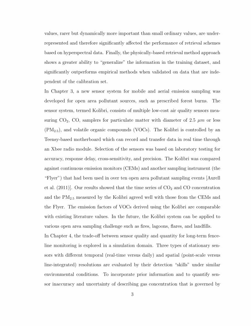
In Chapter 3, a new sensor system for mobile and aerial emission sampling was
developed for open area pollutant sources, such as prescribed forest burns. The
sensor system, termed Kolibri, consists of multiple low-cost air quality sensors mea-
suring CO2, CO, samplers for particulate matter with diameter of 2.5 µm or less
(PM2.5), and volatile organic compounds (VOCs). The Kolibri is controlled by an
Teensy-based motherboard which can record and transfer data in real time through
an Xbee radio module. Selection of the sensors was based on laboratory testing for
accuracy, response delay, cross-sensitivity, and precision. The Kolibri was compared
against continuous emission monitors (CEMs) and another sampling instrument (the
“Flyer”) that had been used in over ten open area pollutant sampling events [Aurell
et al. (2011)]. Our results showed that the time series of CO2 and CO concentration
and the PM2.5 measured by the Kolibri agreed well with those from the CEMs and
the Flyer. The emission factors of VOCs derived using the Kolibri are comparable
with existing literature values. In the future, the Kolibri system can be applied to
various open area sampling challenge such as fires, lagoons, flares, and landfills.
In Chapter 4, the trade-off between sensor quality and quantity for long-term fence-
line monitoring is explored in a simulation domain. Three types of stationary sen-
sors with different temporal (real-time versus daily) and spatial (point-scale versus
line-integrated) resolutions are evaluated by their detection “skills” under similar
environmental conditions. To incorporate prior information and to quantify sen-
sor inaccuracy and uncertainty of describing gas concentration that is governed by
3
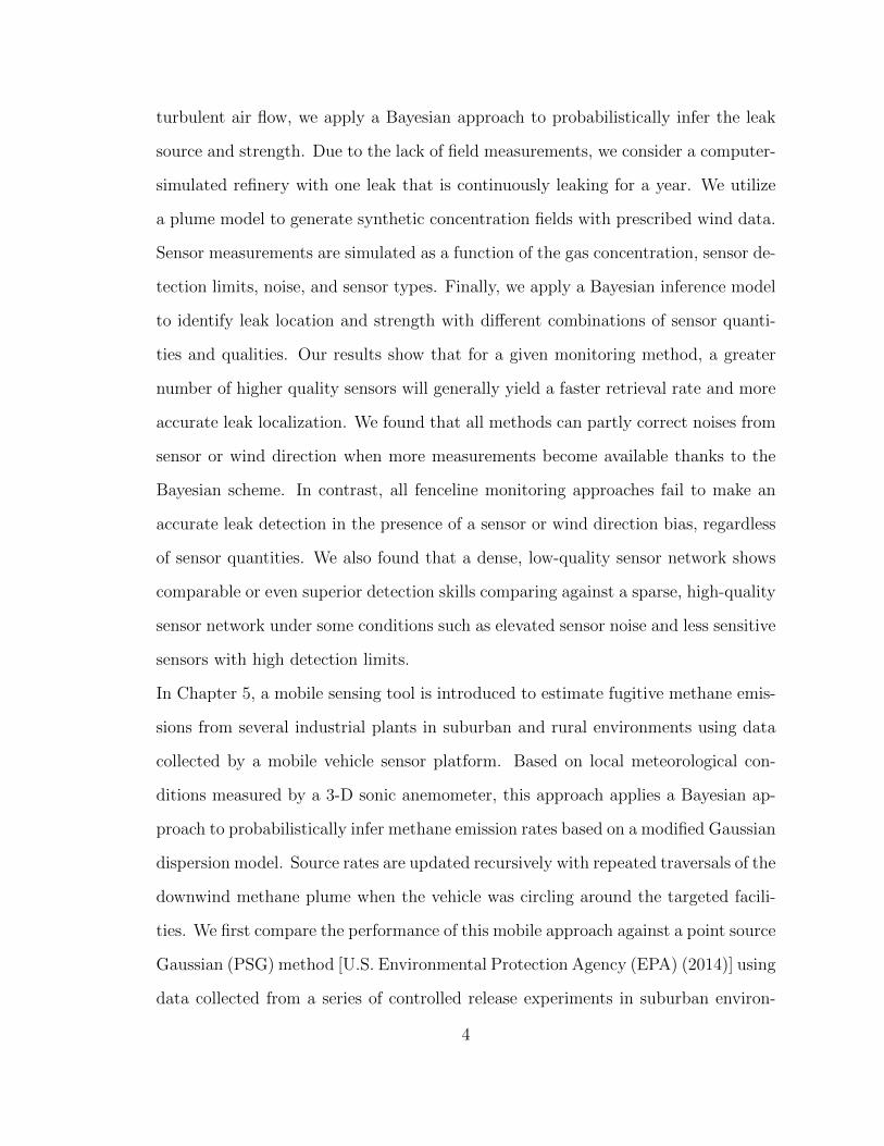
turbulent air flow, we apply a Bayesian approach to probabilistically infer the leak
source and strength. Due to the lack of field measurements, we consider a computer-
simulated refinery with one leak that is continuously leaking for a year. We utilize
a plume model to generate synthetic concentration fields with prescribed wind data.
Sensor measurements are simulated as a function of the gas concentration, sensor de-
tection limits, noise, and sensor types. Finally, we apply a Bayesian inference model
to identify leak location and strength with different combinations of sensor quanti-
ties and qualities. Our results show that for a given monitoring method, a greater
number of higher quality sensors will generally yield a faster retrieval rate and more
accurate leak localization. We found that all methods can partly correct noises from
sensor or wind direction when more measurements become available thanks to the
Bayesian scheme. In contrast, all fenceline monitoring approaches fail to make an
accurate leak detection in the presence of a sensor or wind direction bias, regardless
of sensor quantities. We also found that a dense, low-quality sensor network shows
comparable or even superior detection skills comparing against a sparse, high-quality
sensor network under some conditions such as elevated sensor noise and less sensitive
sensors with high detection limits.
In Chapter 5, a mobile sensing tool is introduced to estimate fugitive methane emis-
sions from several industrial plants in suburban and rural environments using data
collected by a mobile vehicle sensor platform. Based on local meteorological con-
ditions measured by a 3-D sonic anemometer, this approach applies a Bayesian ap-
proach to probabilistically infer methane emission rates based on a modified Gaussian
dispersion model. Source rates are updated recursively with repeated traversals of the
downwind methane plume when the vehicle was circling around the targeted facili-
ties. We first compare the performance of this mobile approach against a point source
Gaussian (PSG) method [U.S. Environmental Protection Agency (EPA) (2014)] using
data collected from a series of controlled release experiments in suburban environ-
4
ments. Results show that the emission rates estimated using the mobile method has
smaller bias and uncertainty comparing against the PSG method. Then, we apply
the mobile sensing approach to quantify fugitive methane emissions from several
ammonia fertilizer plants in rural areas. Significant methane emission was identified
from one facility while the other two shows relatively low emissions. Overall, this
mobile sensing approach shows promising results for future application of quantifying
of fugitive methane emission in suburban and rural environments. With access via
public roads, this mobile monitoring method is able to quickly assess the emission
strength of facilities along the sensor path. This work is developing the capacity
for efficient regional coverage of potential methane emission rates in support of leak
detection and mitigation efforts.
5
2
Remote Sensing Retrieval of Suspended SedimentConcentration in Shallow Coastal Waters
This chapter is based on the article: Zhou, X., Marani, M., Albertson, J. D., and
Silvestri, S., (2015). Hyperspectral and multispectral retrieval of suspended sed-
iment concentration in shallow coastal waters: an applications to the Venice la-
goon.submitted to Remote Sensing of Environment.
2.1 Introduction
The amount of suspended sediment in the water column is a chief determinant of
the state of a water body and of the bio-geomorphic dynamics of aquatic systems.
The Suspended Sediment Concentration (SSC) largely determines water turbidity,
which has important consequences for life such as the survival of seagrass meadows
[Carr et al. (2010)]. On the other hand, suspended sediment supply by rivers and
tidal currents is essential to the survival of intertidal and sub-tidal structures as sea
level rise accelerates [Morris et al. (2002); Marani et al. (2007); Blum and Roberts
(2009); Carniello et al. (2009); D’Alpaos et al. (2011); Kirwan and Megonigal (2013)].
In fact, sediment starvation has been documented to be one of the main sources of
6
ongoing coastal degradation [Ericson et al. (2006); Syvitski et al. (2009); Wang et al.
(2011); Yang et al. (2011)].
Given the importance of the sediment balance in dictating the fate of lagoon and
coastal areas, methods for monitoring of the SSC in a spatially-distributed manner
is vital to understanding and managing these systems. Traditionally, water quality
parameters in coastal and lagoon regions, including the SSC, have been monitored
through point measurements carried out during sporadic field campaigns or through
networks of permanent but sparse monitoring stations. In recent years, the retrieval
of water constituents (e.g. SSC, chlorophyll-a, and colored dissolved organic matter)
using the spectral properties of upwelling radiance leaving the water surface (ocean
color) measured by remote sensors (e.g. SeaWifs, MODIS-Aqua, MERIS, etc.) has
shown considerable success in monitoring deep and oligotrophic open waters [e.g.
Ritchie et al. (2003)]. However, the application of ocean color retrieval approaches
to coastal case II waters, rich in suspended sediments and chlorophylls, faces severe
limitations. This is mainly caused by the spectral complexity of the resulting remote
sensing signal, and the spatial resolutions which are inadequate to resolve hetero-
geneous spatial distributions of water constituents [Moses et al. (2009)]. Despite
its importance, only a few satellite sensors, such as HICO and Landsat OLI, are
specifically designed for water quality monitoring in coastal environments. Though
HICO has an improved spatial resolutions (90 meters), it is not ideal for applying
retrieval approaches in estuaries and shallow lagoon waters. Originally designed for
terrestrial applications, multispectral sensors with higher spatial resolutions, such
as Landsat TM and ETM+, ASTER, and ALOS, have been successfully applied
to SSC retrievals in the coastal zone [Volpe et al. (2011)]. However, their radio-
metric resolution, signal-to-noise ratio, and spectral resolutions pose limits to the
accuracy of remote sensing estimates. One thus wonders whether the optimal selec-
tion of spectral bands from a hyperspectral sensors with sufficient spatial resolution
7
may allow improved retrievals of water constituents in the coastal zone. Currently,
Hyperion (onboard the EO-1 satellite) and CHRIS Proba (onboard ESAs Proba-1
satellite) are the only hyperspectral sensors with a spatial resolution (30m) appro-
priate for coastal water applications [Brando and Dekker (2003); Giardino et al.
(2007); Lee et al. (2007); Santini et al. (2010)]. The planned NASA hyperspectral
mission HyspIRI is expected to launch after 2020 and, thanks to its increased spec-
tral, spatial and radiometric resolutions, will provide high quality data for coastal
water monitoring. However, while rich in information, hyperspectral sensors provide
redundant data for water quality evaluation and need to be carefully analyzed to ex-
tract the useful information. This is true for physically-based models which is based
on mathematical descriptions of the relevant radiative transfer processes [Bajcsy and
Groves (2004)], and for approaches based on empirical relations calibrated on avail-
able observations. Previous studies have used a variety of such physically-based and
empirical approaches. Some approaches used all available hyperspectral bands to es-
timate several water constituents simultaneously [Giardino et al. (2007); Santini et al.
(2010)]. Others used a single hyperspectral band to estimate SSC [Nechad et al.
(2010); Brando and Dekker (2003)] identified, through the sequential exploration of
possible spectral band triplets, the optimal combination of bands (490nm, 670nm,
and 700-740 nm) to simultaneously retrieve SSC, CC, and CDOM . In general, the
band selection results differ significantly among studies and the problem of select-
ing an optimal set of hyperspectral bands for water constituent retrieval in coastal
waters remains an open one. Meanwhile, the relative strengths and weaknesses of
empirical and physically-based approaches are virtually unexplored [Malthus and
Mumby (2003)], and therefore accepted criteria for comparing the performance of
physically-based versus empirical approaches have yet to be established.
In this study, we use a systematic approach to evaluate the performance of empirical
and physically-based methods to retrieve SSC from hyperspectral and multispectral
8
data in the Venice lagoon (Italy). Using this dataset, we are motivated to explore:
strategies to maximize information utilization and minimize the related redundancy
(or error) using hyperspectral data in order to better retrieve SSC in complex Case
II waters; advantages and disadvantages of using hyperspectral data compared with
multispectral data; and performance of SSC retrieval using physically-based model
versus empirically-based models with the same satellite datasets.
2.2 Methods
2.2.1 Study site and datasets
The Venice Lagoon is one of the largest lagoons in Europe with a surface area of about
550 km2 and a watershed of 1,800 km2. It is separated from the Adriatic Sea by two
barrier islands, with three large inlets connecting it to the sea (Fig. 2.1). The lagoon
is relatively shallow, with a mean depth of about 1.2m and a mean semi-diurnal
tidal amplitude of about 0.7m. It includes several islands, with a total surface of 29
km2, salt marshes (covering almost 40 km2), and tidal flats. The lagoon is incised
by a network of canals (total length of about 1,500 km) ranging from shallow (less
than 1 m deep) to very deep (the Malamocco inlet is 22 m deep). Due to a very low
sediment input from the watershed caused by historical river diversions, and to an
asymmetry in the tidally-driven sediment exchange between the sea and the lagoon,
it is currently characterized by strong erosional processes with an annual sediment
deficit of about 400,000 m3. The Venice lagoon is also a eutrophic environment, the
annual quantity of nutrients from the drainage basin includes about 9,000 tons of
organic nitrogen and 1,200 tons of organic phosphorus [Ravera (2000)].
In this study we analyze Hyperion hyperspectral data, and Landsat, ASTER and
ALOS multispectral data. Launched in 2001, Hyperion is onboard the EO-1 satellite
and typically covers a swath of 7.7 km (width) by 42 km (length), with a spectral
coverage from 400 to 2500 nm (FWHM around 10nm) and a spatial resolution of
9
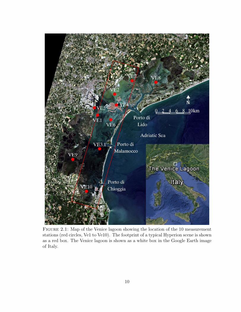
Figure 2.1: Map of the Venice lagoon showing the location of the 10 measurementstations (red circles, Ve1 to Ve10). The footprint of a typical Hyperion scene is shownas a red box. The Venice lagoon is shown as a white box in the Google Earth imageof Italy.
10
30 by 30 meters [Pearlman et al. (2003)]). A set of 5 cloud-free Hyperion scenes, 2
collected in winter and 3 in summer, are used in this study (Table 2.1). Spectral
bands in the 460-700 nm range are selected to constrain the physically-based retrieval
model due to their high sensitivity to water quality variables [Brando and Dekker
(2003)]. In this spectral range, absorption and backscattering coefficients of water
constituents are estimated from local measurements [Santini et al. (2010); Volpe et al.
(2011)]. A set of 13 multispectral images (Landsat TM, Landsat ETM+, ASTER
and ALOS) are also used in this study (Table 2.1) with the purpose of comparing the
quality of hyperspectral and multispectral retrievals. Field data were provided by
the Italian Ministry of Public Works, which monitors the water quality of the Venice
lagoon through a network of 10 multi-parametric probes (Fig. 2.1). Available data
include water pressure, temperature, conductivity, dissolved oxygen, pH, chlorophyll-
a, and turbidity at a 30 minutes interval. Turbidity is measured, at all stations, by
Seapoint optical turbidity meters, which measure the amount of scattering by the
water column in a beam emitted at a wavelength of 880 nm. The amount of scattering
is proportional to the concentration of the matter suspended in the water column.
These turbidity observations are expressed in FTU (Formazine Turbidity Units),
which can be directly related to the SSC (g/m3) [e.g. Old et al. (2002); Volpe
et al. (2011)]. Chlorophyll-a concentration is observed by a Seapoint chlorophyll
fluorometer, which measures the emission spectrum at 685 nm after excitation at
470 nm. Water pressure is measured by a pressure transducer (part of an Ocean
Seven 316 CTD multi-parameter probe). Because the amplitude of tidal fluctuations
is comparable to the mean water depth [Volpe et al. (2011)], pressure data are crucial
to determine the instantaneous water depth, as needed to perform the retrievals. To
match the probe measurements with satellite data, the water quality data at the
satellite overpass time are estimated by linearly interpolating the half-hourly probe
measurements. Due to the limited swath width of Hyperion, typically only 5 to
11
6 probe stations are covered by one Hyperion scene (Fig. 2.1). After excluding
data from stations covered by cloud/haze or affected by malfunctioning probes, we
collect a total of 20 reliable probe measurements for the 5 available Hyperion scenes.
A set of 13 cloud-free multispectral scenes were purposely selected during or right
after extreme wind events in order to maximize the range of SSC values. After
data preprocessing, we obtain a total of 53 reliable probe measurements for further
analysis [Volpe et al. (2011)].
2.2.2 Data processing
The preprocessed Hyperion data (Level 1R) are known to exhibit vertical stripes in
certain spectral bands (provided with the data) due to poorly calibrated detectors
[Datt et al. (2003)]. Here we used an ENVI-plugin Hyperion tool that replaces the
erroneous stripes with a linear interpolation of the adjacent columns [White (2013)].
Data were then atmospherically corrected using the Atmospheric CORrection Now
(ACORN) software, which implements the MODTRAN 4.0 Radiative Transfer Model
developed by the Air Force Research Lab [Acharya et al. (1998)]. ACORN automat-
ically corrects the smile effect, which is a wavelength shift in across-track pixels
mainly caused by push-broom sensor configurations of Hyperion [Green (2001)]. A
mid-latitude, seasonally dependent atmospheric model was applied. The atmospheric
water vapor distribution is estimated by ACORN on a pixel-by-pixel basis using both
the 940 nm and the 1140 nm bands [Gao and Goetz (1990)]. Visibility was assumed
to be spatially homogeneous over the entire scene, and calculated using the aerosol
optical thickness (AOT) values measured by sun-photometers from the AERONET
network [Holben et al. (1998)]. Data from two AERONET sites are used in the
study: the ISDGM-CNR site which located on the roof of a building in central
Venice (45.43698 N, 12.33198 E), and the Venice site which located in the Adriatic
Sea 8 miles offshore from the Venice Lagoon (45.31390 N, 12.50830 E). The aver-
12
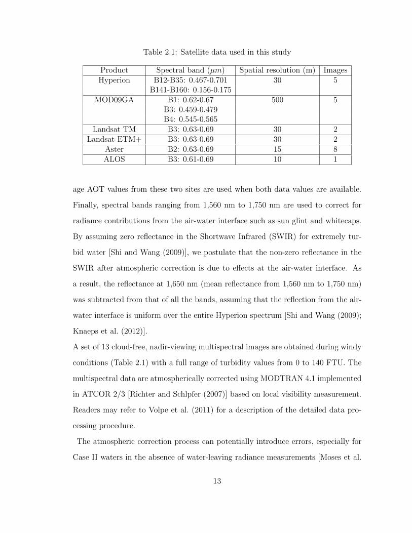
Table 2.1: Satellite data used in this study
Product Spectral band (µm) Spatial resolution (m) ImagesHyperion B12-B35: 0.467-0.701 30 5
B141-B160: 0.156-0.175MOD09GA B1: 0.62-0.67 500 5
B3: 0.459-0.479B4: 0.545-0.565
Landsat TM B3: 0.63-0.69 30 2Landsat ETM+ B3: 0.63-0.69 30 2
Aster B2: 0.63-0.69 15 8ALOS B3: 0.61-0.69 10 1
age AOT values from these two sites are used when both data values are available.
Finally, spectral bands ranging from 1,560 nm to 1,750 nm are used to correct for
radiance contributions from the air-water interface such as sun glint and whitecaps.
By assuming zero reflectance in the Shortwave Infrared (SWIR) for extremely tur-
bid water [Shi and Wang (2009)], we postulate that the non-zero reflectance in the
SWIR after atmospheric correction is due to effects at the air-water interface. As
a result, the reflectance at 1,650 nm (mean reflectance from 1,560 nm to 1,750 nm)
was subtracted from that of all the bands, assuming that the reflection from the air-
water interface is uniform over the entire Hyperion spectrum [Shi and Wang (2009);
Knaeps et al. (2012)].
A set of 13 cloud-free, nadir-viewing multispectral images are obtained during windy
conditions (Table 2.1) with a full range of turbidity values from 0 to 140 FTU. The
multispectral data are atmospherically corrected using MODTRAN 4.1 implemented
in ATCOR 2/3 [Richter and Schlpfer (2007)] based on local visibility measurement.
Readers may refer to Volpe et al. (2011) for a description of the detailed data pro-
cessing procedure.
The atmospheric correction process can potentially introduce errors, especially for
Case II waters in the absence of water-leaving radiance measurements [Moses et al.
13

(2009)]. Hence, we validate our atmospheric correction by comparing the reflectance
obtained from Hyperion with the MODIS surface reflectance product (MOD09GA),
which provides global daily surface reflectance at 500m and 1km resolutions [Ver-
mote and Kotchenova (2008)]. It should be noted that all MODIS data selected
for the comparison were acquired within 30 minutes of the corresponding Hyperion
overpass.
We first simulated MODIS reflectances for band B1, B3, and B4 by resampling the
atmospherically-corrected Hyperion bands falling within the spectral interval of these
bands and by applying the appropriate MODIS spectral response functions. Only
MODIS pixels falling on water were considered in the comparison, and pixels located
at the edge of the lagoon were excluded to avoid effects of mixed land/water pix-
els. For each MODIS pixel (500 by 500 meters), we selected around 256 “synthetic”
MODIS spectra resampled from the Hyperion pixels (30 by 30 meters each) that fell
within it. The mean value of the spectral reflectance of the selected synthetic MODIS
pixels, which we call here the Hyperion Synthetic MODIS (HSM) reflectance, were
used for comparison with the MODIS reflectance.
2.2.3 Radiative transfer model
Above-surface remote sensing reflectance Rrs [sr�1], defined as the ratio of water-
leaving radiance to downwelling irradiance, can be approximated as follows for a
nadir-viewing sensor [Lee et al. (1999)]:
Rrs � 0.5rrs1 � 1.5rrs
(2.1)
where rrs [sr�1] is the below surface remote sensing reflectance in the nadir looking
direction. Following [Lee et al. (1998, 1999)], rrs can be modeled as a function of the
water depth, the optical properties of the water column, and the optical properties
14
of the water bottom:
rrs � rdprs p1 � e�pkd�kcuqHq � ρb
πe�pkd�k
Bu qH (2.2)
where rdprs [sr�1] is the subsurface remote sensing reflectance for an infinitely deep
water, kd [-] is the vertically-averaged diffuse attenuation coefficient for downwelling
irradiance, kcu [-] and kBu [-] are the vertically-averaged diffuse attenuation coefficients
for upwelling irradiance from the water body and from the bottom, respectively. H
is the water depth, and ρb [-] is the bottom reflectance (assuming to be Lambertian).
rdprs , kd, kcu, and kBu can be calculated following [Lee et al. (1999)]:
rdprs �bb
a� bbp0.17
bba� bb
� 0.084q (2.3a)
kd � 1
cospθqpa� bbq (2.3b)
kcu � 1.03pa� bbqc
2.4bb
a� bb(2.3c)
kBu � 1.04pa� bbqc
5.4bb
a� bb(2.3d)
where a [m�1] and bb [m�1] are the total absorption and backscattering coefficients
of water, respectively. θ [rad] is the subsurface solar zenith angle. bb is considered as
a fraction of the total scattering coefficient (b [m�1]). A fixed ratio of bb{b � 0.019 is
adopted from literature [Petzold (1972); Binding et al. (2005); Volpe et al. (2011)].
a and b can be estimated as follows:
a � aw � anap � aph � acdom (2.4a)
b � bw � bnap � bph (2.4b)
where aw [m�1], anap [m�1], aph [m�1], and acdom [m�1] are the absorption coefficients
of pure water, inorganic particles, phytoplankton, and colored dissolved organic mat-
ter, respectively. b is the total scattering coefficient, which can be divided into
15
contributions from pure water (bw [m�1]), inorganic particles (bnap [m�1]), and phy-
toplankton (bph [m�1]). aw is obtained from previous studies [Pope and Fry (1997)].
anap, and aph are modeled as a function of SSC, CC, and their corresponding specific
absorption coefficients a�nappλq and a�phpλq, respectively [Santini et al. (2010); Volpe
et al. (2011)].
anappλq � a�nappλq � SSC (2.5a)
aphpλq � a�phpλq � CC (2.5b)
Field measurements show that a�nappλq follows an exponential decay with increasing
wavelength, while a�phpλq has a bimodal behavior with two peaks located at 430 and
660 nm [e.g. Santini et al. (2010)]. Following Babin et al. (2003a) and Volpe et al.
(2011), we model a�nap as: a�nappλq � λ� 0.75� e�0.0128pλ�443q, in which λ [m2{g] is a
calibration parameter. a�phpλq values are obtained from Santini et al. (2010) and were
measured during a field campaign in the Venice lagoon. We assume that acdompλqalso follows an exponential behavior [Babin et al. (2003b); Volpe et al. (2011)]:
acodmpλq � a�codmpλqe�0.0192pλ�375q (2.6)
where a�cdom is acdom at λ � 375nm. Due to a lack of CDOM measurement specific for
this study, we used a fixed a�cdom � 1.25m�1, which is consistent with field measure-
ments [Ferrari and Tassan (1991)] and other modeling studies [Volpe et al. (2011)]
from the Venice lagoon.
In turbid waters, bw and bph can be neglected with respect to bnap in Eqn. 2.4 [Babin
et al. (2003b); Volpe et al. (2011). Following Volpe et al. (2011), we model bnap as a
function of SSC and its corresponding spectral backscattering spectral coefficients
(b�nappλq).bnappλq � b�nappλq � SSC (2.7)
16
We assume b�nappλq � η�p400{λq0.3q following Haltrin (1998), where η is a calibration
parameter. Combining Eqn. 2.1 to 2.7, we obtain:
SSCE � fRpη, λ, ρb, H, θ, awpλq, a�phpλq, a�cdompλq, CC,Rrspλqq (2.8)
Eqn. 2.8 can be solved numerically to estimate SSC (denoted as SSCE). The
parameters used in Eqn. 2.8, and their typical values, are summarized in Table 2.2.
2.2.4 Empirical retrieval models
Various empirical models have been developed to correlate SSC concentration with
water surface reflectance. Readers may refer to Matthews (2011) for a detailed re-
view. In many cases, a linear regression of SSC with a single red band or with a
NIR/RED ratio shows high correlations, especially for highly turbid waters [e.g.
Lathrop and Lillesand (1989); Doxaran et al. (2002); Miller and McKee (2004);
Doxaran et al. (2005); Tyler et al. (2006); Doxaran et al. (2009); Nechad et al.
(2010)]. Other methods uses log-linear [e.g. Chen et al. (1991)], exponential re-
gressions [e.g. Harrington et al. (1992)], or linear regressions over multiple bands
[Wang and Ma (2001); Wang et al. (2006)]. However, the regression coefficient val-
ues retrieved through in-situ calibration are very site-specific and are not generally
applicable to other datasets. Due to the small range of reflectance (0.01-0.04) and
turbidity data (4-100), typical of the Venice lagoon, we found the log-linear or ex-
ponential models inappropriate. In this study, we apply polynomial functions which
relate SSC with either the reflectance of an individual band, Rrspλq, or with the ra-
tio of reflectance values from pairs of bands, (Rrspλ1q{Rrspλ2q), where the selection
of λ, λ1 and λ2 depends on the available dataset or study site.
SSCE �#fE,1pRrspλqqfE,epRrspλ1q{Rrspλ2qq
(2.9)
17
2.2.5 Calibration and validation
The root mean square error (RMSE) between estimated and measured SSC is used
to evaluate model performance. For the radiative transfer model, in Eqn. 2.8 we
calibrate the absorption and backscattering coefficients of the sediment,(λ, η), to
minimize the RMSE:
RMSE �d°N
1 pSSC � SSCEq2N
(2.10)
where N is the number of measurements.
For the empirical models, we calibrate the coefficients of the polynomial functions
(Eqn. 2.9). To validate the prediction performance of different models, we use
a leave-one-out approach, in which one observation is left out of the calibration
sample and is later used to compute a mean square distance between SSC and
SSCE based on this independent observation. By leaving out for validation, in turn,
each element of the available sample, RMSE can be computed that characterizes the
model predictive abilities [Wilks (2006); Volpe et al. (2011)].
2.2.6 Band selection
As mentioned in the Introduction, the use of hyperspectral data involves the adoption
of a band selection strategy. Brando and Dekker (2003) and Giardino et al. (2007)
used a physically-based retrieval approach to estimate water constituent concentra-
tions through a direct inversion of the bio-optical model, given that the number of
bands equals the number of unknowns. Through trial and error, Brando and Dekker
(2003) select 3 bands (centered at 490 nm, 670 nm, and the average of five bands
from 700-740 nm) for estimating CC, SSC and CDOM . Based on a first-derivative
approach, Giardino et al. (2007) first evaluate the band sensitivity to one water con-
stituent at a time, and then use the average of two groups of bands (480-500 nm
18
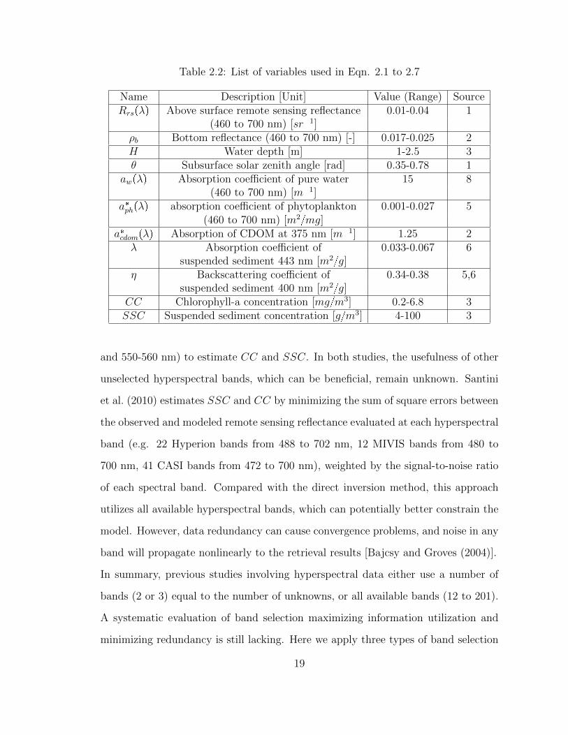
Table 2.2: List of variables used in Eqn. 2.1 to 2.7
Name Description [Unit] Value (Range) SourceRrspλq Above surface remote sensing reflectance 0.01-0.04 1
(460 to 700 nm) [sr�1]ρb Bottom reflectance (460 to 700 nm) [-] 0.017-0.025 2H Water depth [m] 1-2.5 3θ Subsurface solar zenith angle [rad] 0.35-0.78 1
awpλq Absorption coefficient of pure water 15 8(460 to 700 nm) [m�1]
a�phpλq absorption coefficient of phytoplankton 0.001-0.027 5(460 to 700 nm) [m2{mg]
a�cdompλq Absorption of CDOM at 375 nm [m�1] 1.25 2λ Absorption coefficient of 0.033-0.067 6
suspended sediment 443 nm [m2{g]η Backscattering coefficient of 0.34-0.38 5,6
suspended sediment 400 nm [m2{g]CC Chlorophyll-a concentration [mg{m3] 0.2-6.8 3SSC Suspended sediment concentration [g{m3] 4-100 3
and 550-560 nm) to estimate CC and SSC. In both studies, the usefulness of other
unselected hyperspectral bands, which can be beneficial, remain unknown. Santini
et al. (2010) estimates SSC and CC by minimizing the sum of square errors between
the observed and modeled remote sensing reflectance evaluated at each hyperspectral
band (e.g. 22 Hyperion bands from 488 to 702 nm, 12 MIVIS bands from 480 to
700 nm, 41 CASI bands from 472 to 700 nm), weighted by the signal-to-noise ratio
of each spectral band. Compared with the direct inversion method, this approach
utilizes all available hyperspectral bands, which can potentially better constrain the
model. However, data redundancy can cause convergence problems, and noise in any
band will propagate nonlinearly to the retrieval results [Bajcsy and Groves (2004)].
In summary, previous studies involving hyperspectral data either use a number of
bands (2 or 3) equal to the number of unknowns, or all available bands (12 to 201).
A systematic evaluation of band selection maximizing information utilization and
minimizing redundancy is still lacking. Here we apply three types of band selection
19
procedures to calibrate and validate both the radiative transfer model (with two
unknown parameter λ and η in Eqn. 2.8) and the empirical models (up to three
fitting parameters in Eqn. 2.9). First, we use all available bands (24), similar to
Santini et al. (2010). Then, we choose bands centered at 560 nm and 660 nm fol-
lowing Brando and Dekker (2003) and Giardino et al. (2007). The bands centered
at 490 nm were not considered because the blue spectral region presents relatively
more noise compared with other regions [Brando and Dekker (2003); Giardino et al.
(2007)]. Finally, given the model complexity (2-3 unknown parameters), we explore
a subset of band combinations composed of up to 4 bands (°4i�1
�24i
�, where i is the
number of bands). Ideally, all combinations of bands should be tested since a large
number of bands could be beneficial for model calibration. However, we observed
diminishing returns when exploring band combinations up to 4 bands (see Section
3.3), suggesting that an further increase of bands may provide little improvement.
In addition, given the size of our dataset (24 candidate Hyperion bands), further
increasing the number of bands would be computational demanding given the non-
linearity of Eqn. 2.8. As a result, we only tested the band combinations up to 4
bands to relieve the computational burden of the model.
2.3 Results
2.3.1 Atmospheric correction validation
In Fig. 2.2, we plot the reflectance estimated from MODIS against the Hyperion Syn-
thetic MODIS (HSM), with each row of subplots represents different MODIS bands
derived from a single Hyperion scene and each column of subplots represents different
Hyperion scenes with identical MODIS band. The correlation coefficient (COR) and
the Nash-Sutcliffe efficiency (NSE) coefficient [Hash and Sutcliffe (1970)] are calcu-
lated for each subplot to quantify the agreement between the two datasets. For each
subplot, NSE is estimated as: 1�°pMODIS �HSMq2{°pMODIS �MODISq2,
20
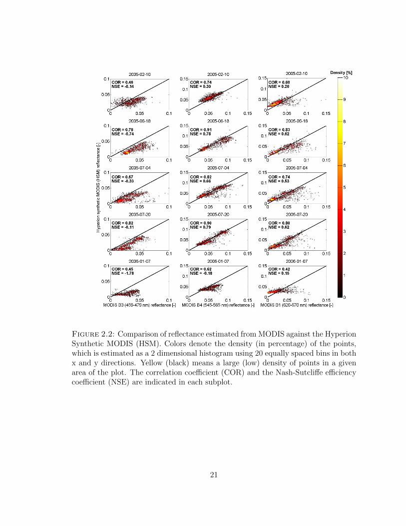
Figure 2.2: Comparison of reflectance estimated from MODIS against the HyperionSynthetic MODIS (HSM). Colors denote the density (in percentage) of the points,which is estimated as a 2 dimensional histogram using 20 equally spaced bins in bothx and y directions. Yellow (black) means a large (low) density of points in a givenarea of the plot. The correlation coefficient (COR) and the Nash-Sutcliffe efficiencycoefficient (NSE) are indicated in each subplot.
21
which ranges from �8 to 1. A NSE value of 1 means a perfect match between
MODIS and HSM, a value of 0 indicates that HSM predicts MODIS as accurate as
its average value (MODIS), and a negative values shows that the predictability of
HSM is worse than MODIS.
The values of the correlation coefficient show that the HSM reflectance is positively
correlated with MODIS reflectance for all data. A scene-to-scene comparison indi-
cates that HSM and MODIS reflectance is less-correlated for data collected in the
winter compared with summer datasets. The 2006-01-07 scene has the lowest re-
flectance across all bands and the smallest COR and NSE values compared with the
remaining scenes. We suggest that this difference may be caused by a very low signal
emerging from the water surfaces due to the small irradiance, which is typical for
winter when the sun elevation in the northern hemisphere is low, and consequently
leads to a lower signal-to-noise ratio (SNR) in winter season compared with sum-
mer. A band-to-band comparison shows that the NSE values are generally highest
for band 4 (545-565 nm), medium for band 1 (620-670 nm) and lowest for band 3
(459-479 nm). This can be attributed to the fact that the spectral reflectance of a
water surface tends to be higher in the green part of the spectrum compared with red
and blue reflectances. Also, the Hyperion data were found to be more noisy in the
blue part of the spectrum [Brando and Dekker (2003); Giardino et al. (2007)], which
potentially leads to a low NSE and COR for this band. Given the different spec-
tral and spatial resolution, the difference in the acquisition times ( 30 minutes), and
the uncertainties associated with the atmospheric correction algorithm and the con-
struction of the synthetic bands, the generally good agreement between MODIS and
HSM reflectances gives us confidence in the accuracy of the atmospheric correction
procedure applied to the Hyperion data.
22
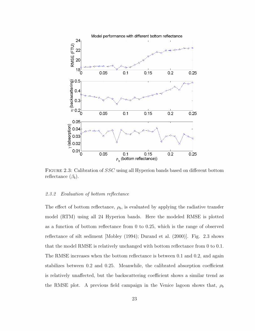
Figure 2.3: Calibration of SSC using all Hyperion bands based on different bottomreflectance (βb).
2.3.2 Evaluation of bottom reflectance
The effect of bottom reflectance, ρb, is evaluated by applying the radiative transfer
model (RTM) using all 24 Hyperion bands. Here the modeled RMSE is plotted
as a function of bottom reflectance from 0 to 0.25, which is the range of observed
reflectance of silt sediment [Mobley (1994); Durand et al. (2000)]. Fig. 2.3 shows
that the model RMSE is relatively unchanged with bottom reflectance from 0 to 0.1.
The RMSE increases when the bottom reflectance is between 0.1 and 0.2, and again
stabilizes between 0.2 and 0.25. Meanwhile, the calibrated absorption coefficient
is relatively unaffected, but the backscattering coefficient shows a similar trend as
the RMSE plot. A previous field campaign in the Venice lagoon shows that, ρb
23
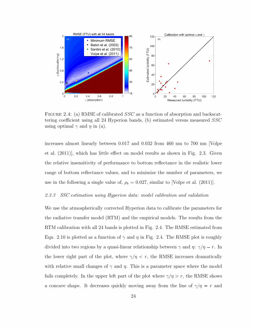
Figure 2.4: (a) RMSE of calibrated SSC as a function of absorption and backscat-tering coefficient using all 24 Hyperion bands, (b) estimated versus measured SSCusing optimal γ and η in (a).
increases almost linearly between 0.017 and 0.032 from 460 nm to 700 nm [Volpe
et al. (2011)], which has little effect on model results as shown in Fig. 2.3. Given
the relative insensitivity of performance to bottom reflectance in the realistic lower
range of bottom reflectance values, and to minimize the number of parameters, we
use in the following a single value of, ρb = 0.027, similar to [Volpe et al. (2011)].
2.3.3 SSC estimation using Hyperion data: model calibration and validation
We use the atmospherically corrected Hyperion data to calibrate the parameters for
the radiative transfer model (RTM) and the empirical models. The results from the
RTM calibration with all 24 bands is plotted in Fig. 2.4. The RMSE estimated from
Eqn. 2.10 is plotted as a function of γ and η in Fig. 2.4. The RMSE plot is roughly
divided into two regions by a quasi-linear relationship between γ and η: γ{η � r. In
the lower right part of the plot, where γ{η r, the RMSE increases dramatically
with relative small changes of γ and η. This is a parameter space where the model
fails completely. In the upper left part of the plot where γ{η ¡ r, the RMSE shows
a concave shape. It decreases quickly moving away from the line of γ{η � r and
24
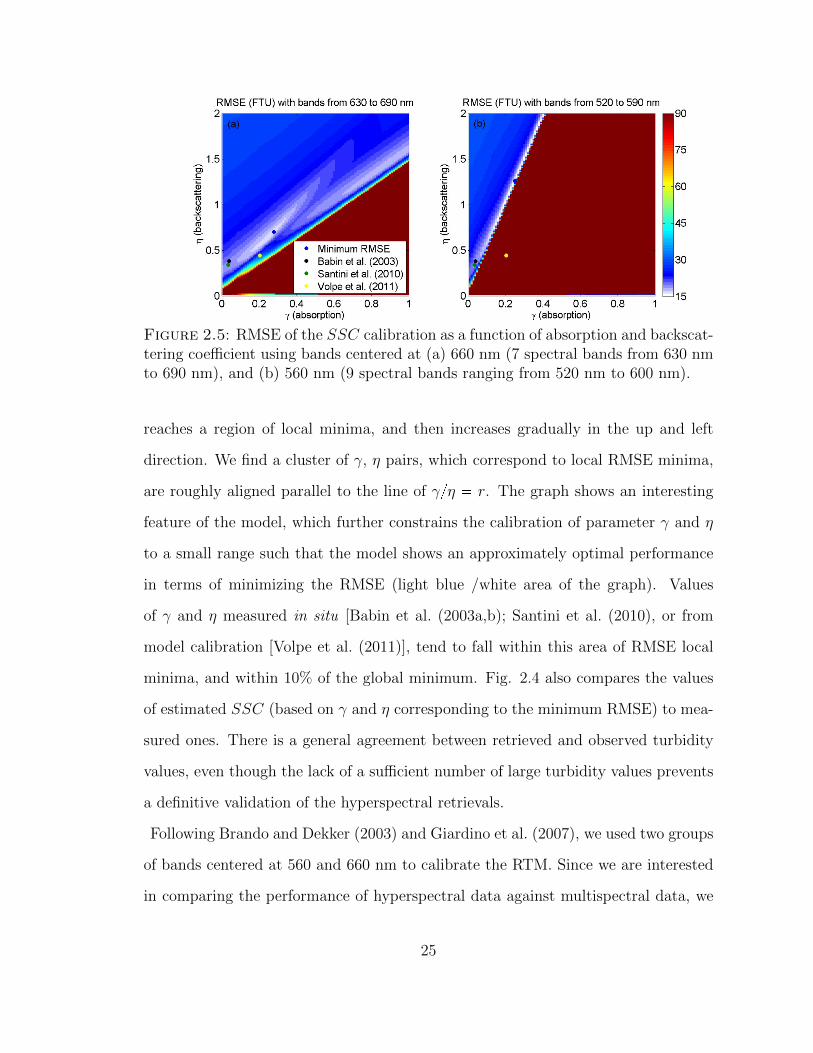
Figure 2.5: RMSE of the SSC calibration as a function of absorption and backscat-tering coefficient using bands centered at (a) 660 nm (7 spectral bands from 630 nmto 690 nm), and (b) 560 nm (9 spectral bands ranging from 520 nm to 600 nm).
reaches a region of local minima, and then increases gradually in the up and left
direction. We find a cluster of γ, η pairs, which correspond to local RMSE minima,
are roughly aligned parallel to the line of γ{η � r. The graph shows an interesting
feature of the model, which further constrains the calibration of parameter γ and η
to a small range such that the model shows an approximately optimal performance
in terms of minimizing the RMSE (light blue /white area of the graph). Values
of γ and η measured in situ [Babin et al. (2003a,b); Santini et al. (2010), or from
model calibration [Volpe et al. (2011)], tend to fall within this area of RMSE local
minima, and within 10% of the global minimum. Fig. 2.4 also compares the values
of estimated SSC (based on γ and η corresponding to the minimum RMSE) to mea-
sured ones. There is a general agreement between retrieved and observed turbidity
values, even though the lack of a sufficient number of large turbidity values prevents
a definitive validation of the hyperspectral retrievals.
Following Brando and Dekker (2003) and Giardino et al. (2007), we used two groups
of bands centered at 560 and 660 nm to calibrate the RTM. Since we are interested
in comparing the performance of hyperspectral data against multispectral data, we
25
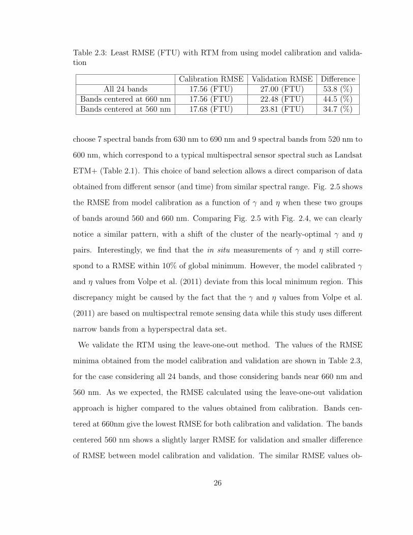
Table 2.3: Least RMSE (FTU) with RTM from using model calibration and valida-tion
Calibration RMSE Validation RMSE DifferenceAll 24 bands 17.56 (FTU) 27.00 (FTU) 53.8 (%)
Bands centered at 660 nm 17.56 (FTU) 22.48 (FTU) 44.5 (%)Bands centered at 560 nm 17.68 (FTU) 23.81 (FTU) 34.7 (%)
choose 7 spectral bands from 630 nm to 690 nm and 9 spectral bands from 520 nm to
600 nm, which correspond to a typical multispectral sensor spectral such as Landsat
ETM+ (Table 2.1). This choice of band selection allows a direct comparison of data
obtained from different sensor (and time) from similar spectral range. Fig. 2.5 shows
the RMSE from model calibration as a function of γ and η when these two groups
of bands around 560 and 660 nm. Comparing Fig. 2.5 with Fig. 2.4, we can clearly
notice a similar pattern, with a shift of the cluster of the nearly-optimal γ and η
pairs. Interestingly, we find that the in situ measurements of γ and η still corre-
spond to a RMSE within 10% of global minimum. However, the model calibrated γ
and η values from Volpe et al. (2011) deviate from this local minimum region. This
discrepancy might be caused by the fact that the γ and η values from Volpe et al.
(2011) are based on multispectral remote sensing data while this study uses different
narrow bands from a hyperspectral data set.
We validate the RTM using the leave-one-out method. The values of the RMSE
minima obtained from the model calibration and validation are shown in Table 2.3,
for the case considering all 24 bands, and those considering bands near 660 nm and
560 nm. As we expected, the RMSE calculated using the leave-one-out validation
approach is higher compared to the values obtained from calibration. Bands cen-
tered at 660nm give the lowest RMSE for both calibration and validation. The bands
centered 560 nm shows a slightly larger RMSE for validation and smaller difference
of RMSE between model calibration and validation. The similar RMSE values ob-
26
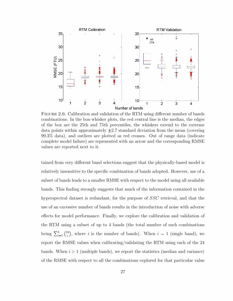
Figure 2.6: Calibration and validation of the RTM using different number of bandscombinations. In the box-whisker plots, the red central line is the median, the edgesof the box are the 25th and 75th percentiles, the whiskers extend to the extremedata points within approximately �2.7 standard deviation from the mean (covering99.3% data), and outliers are plotted as red crosses. Out of range data (indicatecomplete model failure) are represented with an arrow and the corresponding RMSEvalues are reported next to it.
tained from very different band selections suggest that the physically-based model is
relatively insensitive to the specific combination of bands adopted. However, use of a
subset of bands leads to a smaller RMSE with respect to the model using all available
bands. This finding strongly suggests that much of the information contained in the
hyperspectral dataset is redundant, for the purpose of SSC retrieval, and that the
use of an excessive number of bands results in the introduction of noise with adverse
effects for model performance. Finally, we explore the calibration and validation of
the RTM using a subset of up to 4 bands (the total number of such combinations
being°4i�1
�24i
�, where i is the number of bands). When i � 1 (single band), we
report the RMSE values when calibrating/validating the RTM using each of the 24
bands. When i ¡ 1 (multiple bands), we report the statistics (median and variance)
of the RMSE with respect to all the combinations explored for that particular value
27

of i. We plot in Fig. 2.6 the modeled RMSE as a function of the number of bands
used for both model calibration and validation. It shows that the combination of
two bands performs nearly as well as the combination of three or four bands in terms
of minimum and median RMSE for both model calibration and validation, showing
that adding bands does not significantly improve the model performance. This can
be further validated when comparing with the RMSE estimated using all available
bands and two groups of bands recommended by other studies (Table 2.3). Compared
with the cases of 2-4 bands combinations, the single band method has higher data
variability around the median. Though the single band approach yields the smallest
median and minimum RMSE for model calibration, its performance decreases dra-
matically in the model validation. In contrast, for both calibration and validation,
2-4 bands combinations show more robust performance and are more consistent than
the single band approach. These results can be interpreted by considering that the
two underlying parameters remain poorly constrained when just one band is used in
the calibration/validation process (even though the system is still over-determined,
since as many conditions as observations, i.e. 20, are imposed in the calculation of
the RMSE). Using more than two bands is found not to improve retrieval perfor-
mance.
To explore the relative performance of each of the 24 bands for calibrating and val-
idating the RTM, we calculate the RMSE for the different band combinations (Fig.
2.7). In the case of 2-4 bands combinations, the statistics (mean, minimum, and
standard deviation) of a band centered at a specific wavelength is computed using
all the possible combinations of that band with the others. In general, the results
confirm that even if the single band method performs slightly better in calibration,
it performs clearly worse in validation when compared with the multiple band com-
binations (Fig. 2.7). For the single band case, there are four bands (528 nm, 589
nm, 640 nm, and 701 nm) that yield locally-optimal and consistent performance for
28
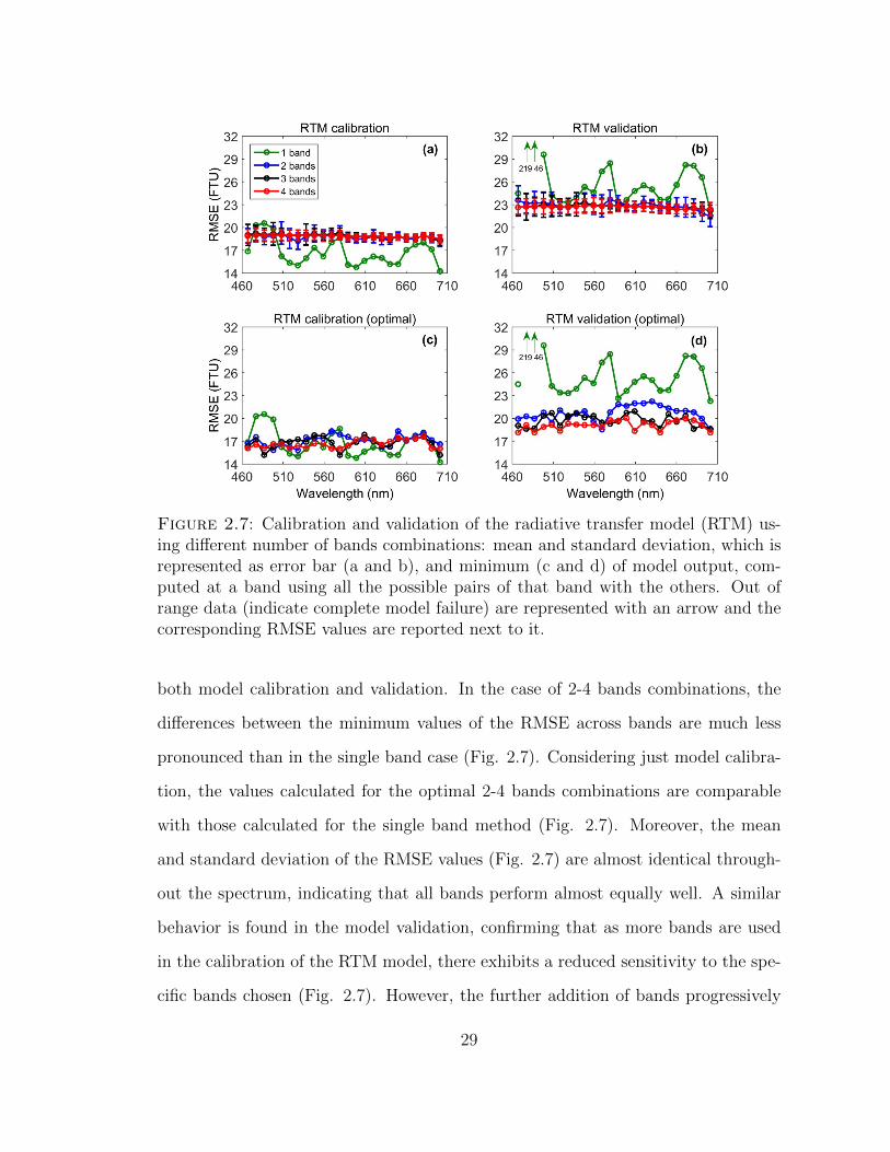
Figure 2.7: Calibration and validation of the radiative transfer model (RTM) us-ing different number of bands combinations: mean and standard deviation, which isrepresented as error bar (a and b), and minimum (c and d) of model output, com-puted at a band using all the possible pairs of that band with the others. Out ofrange data (indicate complete model failure) are represented with an arrow and thecorresponding RMSE values are reported next to it.
both model calibration and validation. In the case of 2-4 bands combinations, the
differences between the minimum values of the RMSE across bands are much less
pronounced than in the single band case (Fig. 2.7). Considering just model calibra-
tion, the values calculated for the optimal 2-4 bands combinations are comparable
with those calculated for the single band method (Fig. 2.7). Moreover, the mean
and standard deviation of the RMSE values (Fig. 2.7) are almost identical through-
out the spectrum, indicating that all bands perform almost equally well. A similar
behavior is found in the model validation, confirming that as more bands are used
in the calibration of the RTM model, there exhibits a reduced sensitivity to the spe-
cific bands chosen (Fig. 2.7). However, the further addition of bands progressively
29
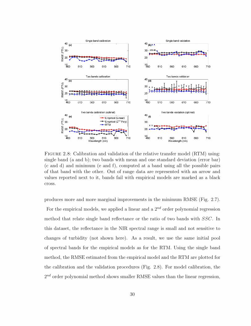
Figure 2.8: Calibration and validation of the relative transfer model (RTM) using:single band (a and b); two bands with mean and one standard deviation (error bar)(c and d) and minimum (e and f), computed at a band using all the possible pairsof that band with the other. Out of range data are represented with an arrow andvalues reported next to it, bands fail with empirical models are marked as a blackcross.
produces more and more marginal improvements in the minimum RMSE (Fig. 2.7).
For the empirical models, we applied a linear and a 2nd order polynomial regression
method that relate single band reflectance or the ratio of two bands with SSC. In
this dataset, the reflectance in the NIR spectral range is small and not sensitive to
changes of turbidity (not shown here). As a result, we use the same initial pool
of spectral bands for the empirical models as for the RTM. Using the single band
method, the RMSE estimated from the empirical model and the RTM are plotted for
the calibration and the validation procedures (Fig. 2.8). For model calibration, the
2nd order polynomial method shows smaller RMSE values than the linear regression,
30
partly due to its additional degree of freedom. However, the linear regression gives
smaller RMSE values than the 2nd polynomial method in the validation. Meanwhile,
the RTM with one band has the least RMSE values for model calibration, and similar
RMSE values for most of the bands compared with the linear regression method in
model validation mode. Overall, when a single band method is selected, the RTM
and the empirical models have similar performances.
Fig. 2.8 shows that the linear regression of the band-ratio has slightly larger (smaller)
mean RMSE compared with the 2nd order polynomial regression method for calibra-
tion (validation). However, the linear regression method has much less variance and
thus it is more robust compared with the 2nd order polynomial method. In addi-
tion, the optimal RMSE values obtained for the 2nd order polynomial method are
smaller than those obtained with the linear regression method for both calibration
and validation (Fig. 2.8) across wavelengths. These results show that the 2nd order
polynomial regression of band ratios has a better performance in terms of RMSE.
However this method is sensitive to band selections. Comparing both linear and 2nd
order polynomial regression with the RTM, the RTM has smaller mean RMSE and
variance for both model calibration and validation; slightly higher (similar) optimal
RMSE for calibration (validation). This comparison suggests that the RTM method
with two bands has superior performances compared with both linear and 2nd poly-
nomial regression when the band ratio is optimally selected.
Based on these results, the linear and 2nd order polynomial empirical models with
either single band or band ratio cannot achieve equivalent performance (in terms of
mean, least, and variance of RMSE for both calibration and leave-one-out validation)
as the RTM with one or two bands. Though the RTM is not robust as may have
been expected, it is the most reliable approach according to our analyses.
31
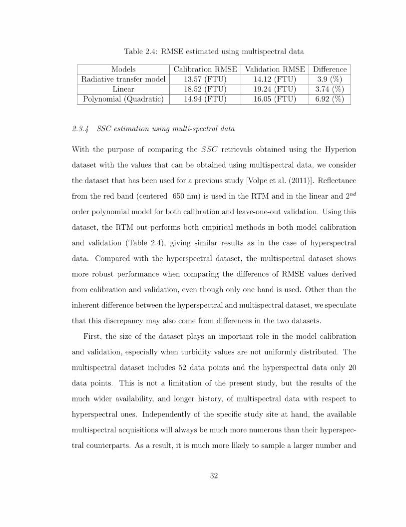
Table 2.4: RMSE estimated using multispectral data
Models Calibration RMSE Validation RMSE DifferenceRadiative transfer model 13.57 (FTU) 14.12 (FTU) 3.9 (%)
Linear 18.52 (FTU) 19.24 (FTU) 3.74 (%)Polynomial (Quadratic) 14.94 (FTU) 16.05 (FTU) 6.92 (%)
2.3.4 SSC estimation using multi-spectral data
With the purpose of comparing the SSC retrievals obtained using the Hyperion
dataset with the values that can be obtained using multispectral data, we consider
the dataset that has been used for a previous study [Volpe et al. (2011)]. Reflectance
from the red band (centered 650 nm) is used in the RTM and in the linear and 2nd
order polynomial model for both calibration and leave-one-out validation. Using this
dataset, the RTM out-performs both empirical methods in both model calibration
and validation (Table 2.4), giving similar results as in the case of hyperspectral
data. Compared with the hyperspectral dataset, the multispectral dataset shows
more robust performance when comparing the difference of RMSE values derived
from calibration and validation, even though only one band is used. Other than the
inherent difference between the hyperspectral and multispectral dataset, we speculate
that this discrepancy may also come from differences in the two datasets.
First, the size of the dataset plays an important role in the model calibration
and validation, especially when turbidity values are not uniformly distributed. The
multispectral dataset includes 52 data points and the hyperspectral data only 20
data points. This is not a limitation of the present study, but the results of the
much wider availability, and longer history, of multispectral data with respect to
hyperspectral ones. Independently of the specific study site at hand, the available
multispectral acquisitions will always be much more numerous than their hyperspec-
tral counterparts. As a result, it is much more likely to sample a larger number and
32
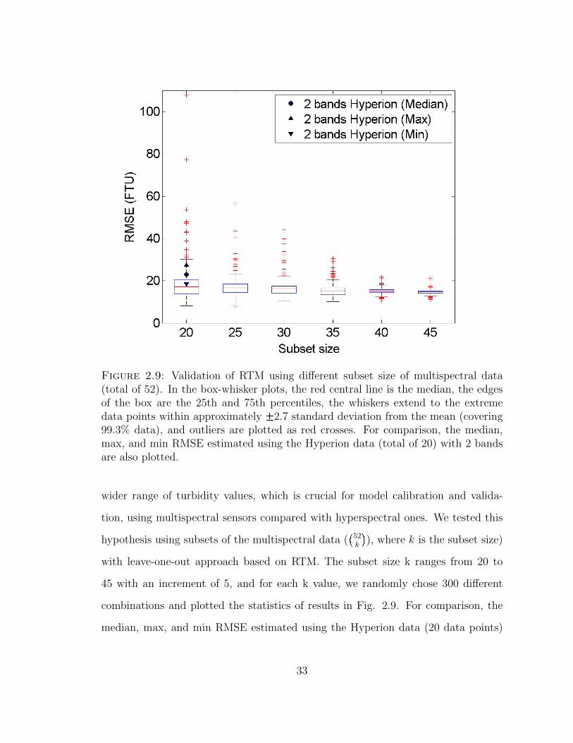
Figure 2.9: Validation of RTM using different subset size of multispectral data(total of 52). In the box-whisker plots, the red central line is the median, the edgesof the box are the 25th and 75th percentiles, the whiskers extend to the extremedata points within approximately �2.7 standard deviation from the mean (covering99.3% data), and outliers are plotted as red crosses. For comparison, the median,max, and min RMSE estimated using the Hyperion data (total of 20) with 2 bandsare also plotted.
wider range of turbidity values, which is crucial for model calibration and valida-
tion, using multispectral sensors compared with hyperspectral ones. We tested this
hypothesis using subsets of the multispectral data (�
52k
�), where k is the subset size)
with leave-one-out approach based on RTM. The subset size k ranges from 20 to
45 with an increment of 5, and for each k value, we randomly chose 300 different
combinations and plotted the statistics of results in Fig. 2.9. For comparison, the
median, max, and min RMSE estimated using the Hyperion data (20 data points)
33
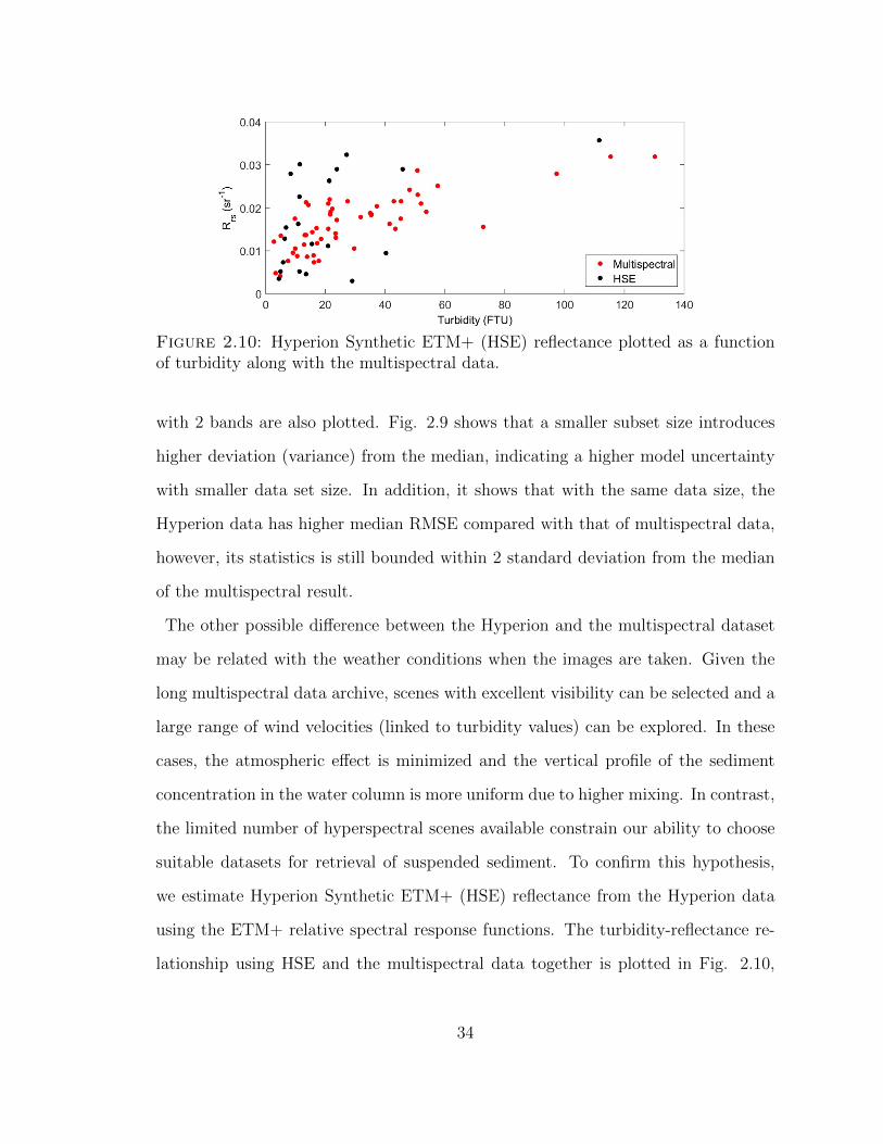
Figure 2.10: Hyperion Synthetic ETM+ (HSE) reflectance plotted as a functionof turbidity along with the multispectral data.
with 2 bands are also plotted. Fig. 2.9 shows that a smaller subset size introduces
higher deviation (variance) from the median, indicating a higher model uncertainty
with smaller data set size. In addition, it shows that with the same data size, the
Hyperion data has higher median RMSE compared with that of multispectral data,
however, its statistics is still bounded within 2 standard deviation from the median
of the multispectral result.
The other possible difference between the Hyperion and the multispectral dataset
may be related with the weather conditions when the images are taken. Given the
long multispectral data archive, scenes with excellent visibility can be selected and a
large range of wind velocities (linked to turbidity values) can be explored. In these
cases, the atmospheric effect is minimized and the vertical profile of the sediment
concentration in the water column is more uniform due to higher mixing. In contrast,
the limited number of hyperspectral scenes available constrain our ability to choose
suitable datasets for retrieval of suspended sediment. To confirm this hypothesis,
we estimate Hyperion Synthetic ETM+ (HSE) reflectance from the Hyperion data
using the ETM+ relative spectral response functions. The turbidity-reflectance re-
lationship using HSE and the multispectral data together is plotted in Fig. 2.10,
34
where it is clearly shown that the HSE data is more scattered in the low turbidity
range, and has only one high turbidity point. In contrast, the multi-spectral data
more uniformly sample the turbidity-reflectance space, with multiple high turbidity
data points. We calibrated and validated both RTM and empirical model with the
combined HSE and multispectral data, and the results show that the inclusion of
the HSE data will increase the model RMSE with respect to case of using only the
multispectral data. In conclusion, the hyperspectral data are highly scattered and
provide a less robust turbidity-reflectance correlation compared with multispectral
data.
2.4 Conclusion and Discussion
This study used a systematic approach to assess the performance of several empiri-
cal methods and a semi-analytic radiative transfer model (RTM) for the retrieval of
suspended sediment concentration (SSC) in a shallow water environment using both
hyperspectral and multispectral data. First, we found a dependence between the ab-
sorption and backscattering coefficients in calibrating the RTM, which is consistent
with literature values (Fig. 2.4 and Fig. 2.5). This result can help constrain the
parameter space in the model calibration phase. We then explored the effects of in-
formation redundancy and band selection for the RTM for calibration and validation.
Our results show that with two calibration parameters, a two-band approach pro-
vides sufficient performance in terms of mean and minimum RMSE for both model
calibration and validation. The two band approach shows more robust performance
and less sensitivity to band selection compared with the use of a single band, espe-
cially in the validation phase using the leave-one-out approach. Additional bands
(three or four) do not improve the model performance significantly. Comparisons
between the RTM and two empirical models (linear and 2nd order polynomial re-
gressions) show that the RTM is more reliable in terms of minimum, median, and
35
variance of RMSE estimated from both model calibration and validation. When
compared to a set of multispectral data, the hyperspectral data showed a limited
ability of predicting SSC. We speculate that the inferior performance of the Hy-
perion data comes from two possible sources: lack of long-term measurements and
suitable datasets. To confirm our hypothesis of data availability, we used subsets
of the multispectral data and found that a larger data size can better constrain the
model and cause less uncertainty in the retrieval. Given the same sizes for multi-
spectral and hyperspectral data, retrievals using hyperspectral data are comparable
with those obtained from multispectral data. To explore the effect of data qual-
ity, we compared the turbidity-reflectance relationship using the Hyperion Synthetic
ETM+ (HSE) reflectance and the multispectral data. The results show that HSE
data is more scattered and strongly skewed towards low turbidity, indicating that the
hyperspectral dataset is less suitable for estimating suspended sediment compared
with the multispectral data. Hence, on one hand the availability of a larger number
of bands does not provide significant improvements in the estimation of SSC, on the
other, the smaller number of hyperspectral acquisitions available at any given site
very significantly limits the possibility of establishing a robust observational relation
between SSC and remote sensing reflectance.
With the two RMSE values estimated from the same dataset using model calibra-
tion and leave-one-out validation, we give more weight to the validation result when
evaluating model performance since it is a more robust estimator to assess model’s
predictability especially when the size of dataset is relatively small. When comparing
the RTM against empirical models (linear and a 2nd order polynomial regressions),
we found out that the RTM with one band has the least RMSE values with model
calibration mode, and similar RMSE values for most bands compared with the em-
pirical methods in model validation mode. Overall, given a single spectral band,
the RTM has slightly better performance compared with empirical methods. Com-
36
paring against linear and 2nd order polynomial regression of band ratios, the RTM
with 2 bands has smaller mean RMSE and variance for both model calibration and
validation (Fig. 2.8). This comparison suggests that compared with both linear
and 2nd polynomial regression methods, the RTM method has a wider applicabil-
ity and robust performance with respect to band selections. This attribute can be
beneficial when the ideal bands suffer from low SNR due to sensor characteristics
or atmospheric conditions, less preferable band combinations can be used without
introducing a significant error. When bands are optimally selected, the RTM has
a slightly higher (similar) RMSE for calibration (validation) as shown in Fig. 2.8,
respectively. This suggests that even though RTM has inferior data fitting skills, it
has equally accurate predictability compared against empirical model. In sum, we
conclude that the RTM has superior performances compared with both linear and
2nd polynomial regression methods with two bands.
Though we used only one multispectral band for model calibration and validation, it
shows superior and more robust performance compared with the hyperspectral data
regardless of model and band selections. In this case, the high spectral resolution
doesnt improve the retrieval of SSC significantly. More specifically, we found that
the use of two bands is sufficient to achieve good performance. In contrast, we found
that a larger size dataset can significantly reduce retrieval uncertainty (Fig. 2.9). In
sum, we did not find a trade-off between number of spectral bands and number of
data points with hyperspectral dataset for estimating SSC. As a result, the lack of
a long archive dataset may jeopardize the usefulness of the hyperspectral data for
monitoring SSC. We have only five cloud-free Hyperion images, which include a
total of 20 pixels coincide with valid probe measurement. With such a small number
of measurement data, the uncertainty of atmospheric correction and probe data will
cause significant errors in model results. In addition, the RMSE method will give
more weight towards the high turbidity values, and the probe measured turbidity
37
is highly skewed towards low values. This mismatch will cause a high dependence
of model accuracy on the large turbidity data points. In contrast, there are much
longer historical archive of multispectral images that are publically available. For
retrieving suspended sediment in shallow lagoon, remote sensing scenes taken during
cloud-free and windy summer time are ideal. In these conditions, the uncertainty of
atmospheric correction is be minimized because of the high visibility and relatively
large surface reflectance due to small sun angle in summer time. Wind shear will
enhance sediment re-suspension from river bed and the in situ sensor can detect
larger turbidity values, which can better help model calibration and validation.
Hyperspectral images have shown considerable success when evaluating concentra-
tions of water constituents in coastal regions and lagoons using data collected during
field campaigns [Brando and Dekker (2003); Giardino et al. (2007); Lee et al. (2007);
Santini et al. (2010)]. However, this study implies that larger archives of hyperspec-
tral data are needed to provide a solid retrieval of suspended sediment when the
models are forced with in situ probe data. To our knowledge, the Venice lagoon is
one of the most densely monitored lagoon system in the world, but we still face the
challenge of obtaining enough data to validate our model. As a result, we anticipate
the remote sensing retrieval of suspended sediment using in situ data with hyper-
spectral image to be further deteriorated in other shallow water systems with sparse,
short-term monitoring stations. Up until now, multispectral data with longer data
archive is more valuable for long-term monitoring suspended sediment in shallow
waters compared with hyperspectral images.
38
3
Development and Evaluation of a LightweightSensor System for Aerial Emission Sampling from
Open Area Sources
This chapter is based on the article: Zhou, X., Aurell, J., Mitchell, W., Tabor, D.,
and Gullett, B., A lightweight sensor/sampler system for aerial emission sampling
from open area sources, under preparation
3.1 Introduction
Open burning, particularly forest and agricultural fires, is one of the largest sources
of trace gases and aerosol particles in the atmosphere and plays an important role
in the atmospheric chemistry and climate by affecting chemical composition, ra-
diation budget, and biogeochemical cycles [Crutzen and Andreae (1990); Andreae
and Merlet (2001); Bond et al. (2004)]. To better understand its impact on human
health and climate system, various models have characterized this process quanti-
tatively based on emission factors, which are the amount of pollutant quantity per
unit amount of the raw material burned (e.g., biomass) [Reid et al. (2005)]. Emission
39
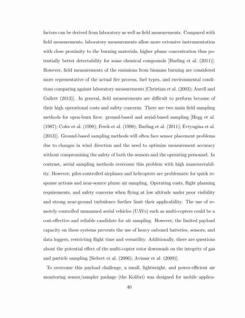
factors can be derived from laboratory as well as field measurements. Compared with
field measurements, laboratory measurements allow more extensive instrumentation
with close proximity to the burning materials, higher plume concentration thus po-
tentially better detectability for some chemical compounds [Burling et al. (2011)].
However, field measurements of the emissions from biomass burning are considered
more representative of the actual fire process, fuel types, and environmental condi-
tions comparing against laboratory measurements [Christian et al. (2003); Aurell and
Gullett (2013)]. In general, field measurements are difficult to perform because of
their high operational costs and safety concerns. There are two main field sampling
methods for open-burn fires: ground-based and aerial-based sampling [Hegg et al.
(1987); Cofer et al. (1998); Ferek et al. (1998); Burling et al. (2011); Evtyugina et al.
(2013)]. Ground-based sampling methods will often face sensor placement problems
due to changes in wind direction and the need to optimize measurement accuracy
without compromising the safety of both the sensors and the operating personnel. In
contrast, aerial sampling methods overcome this problem with high maneuverabil-
ity. However, pilot-controlled airplanes and helicopters are problematic for quick re-
sponse actions and near-source plume air sampling. Operating costs, flight planning
requirements, and safety concerns when flying at low altitude under poor visibility
and strong near-ground turbulence further limit their applicability. The use of re-
motely controlled unmanned aerial vehicles (UAVs) such as multi-copters could be a
cost-effective and reliable candidate for air sampling. However, the limited payload
capacity on these systems prevents the use of heavy onboard batteries, sensors, and
data loggers, restricting flight time and versatility. Additionally, there are questions
about the potential effect of the multi-copter rotor downwash on the integrity of gas
and particle sampling [Siebert et al. (2006); Avissar et al. (2009)].
To overcome this payload challenge, a small, lightweight, and power-efficient air
monitoring sensor/sampler package (the Kolibri) was designed for mobile applica-
40
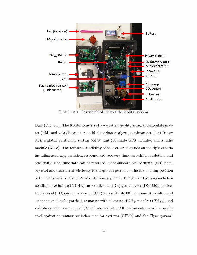
Figure 3.1: Disassembled view of the Kolibri system
tions (Fig. 3.1). The Kolibri consists of low-cost air quality sensors, particulate mat-
ter (PM) and volatile samplers, a black carbon analyzer, a microcontroller (Teensy
3.1), a global positioning system (GPS) unit (Ultimate GPS module), and a radio
module (Xbee). The technical feasibility of the sensors depends on multiple criteria
including accuracy, precision, response and recovery time, zero-drift, resolution, and
sensitivity. Real-time data can be recorded in the onboard secure digital (SD) mem-
ory card and transferred wirelessly to the ground personnel, the latter aiding position
of the remote-controlled UAV into the source plume. The onboard sensors include a
nondispersive infrared (NDIR) carbon dioxide (CO2) gas analyzer (DX6220), an elec-
trochemical (EC) carbon monoxide (CO) sensor (EC4-500), and miniature filter and
sorbent samplers for particulate matter with diameter of 2.5 µm or less (PM2.5), and
volatile organic compounds (VOCs), respectively. All instruments were first evalu-
ated against continuous emission monitor systems (CEMs) and the Flyer system1
41
in an Open Burn Test Facility (OBTF). Measurement accuracy, noise, response and
recovery time, and zero-drift were quantified to ensure the system’s applicability to
the transient nature of some open area emission events.
3.2 Method
A new sensor system was designed to measure CO, CO2, PM2.5 and VOC using cri-
teria of technical feasibility, low weight, and limited power consumption. The sensor
response time and recovery time are particularly challenging for sensors in appli-
cations such as forest fires where the concentrations rapidly fluctuate and response
delays are unacceptable. The limitation on sensor/sampler weight is particularly crit-
ical for UAV applications to maximize flight time. In addition, sensor selectivity is
particularly important as many sensors are affected by other pollutants as well as rel-
ative humidity and temperature. The technical feasibility of select sensors/samplers
are evaluated in this paper against benchmark CEMs and calibration gases.
The CO2 concentration on the Kolibri is measured by a NDIR gas analyzer (DX6220)
manufactured by RMT Ltd., Moscow, Russian. It has a measurement range from 0
to 20% (1% = 10,000 ppm). Its rated accuracy (noise) is 20 (10) ppm when CO2
concentration is less than 1,000 ppm and 1% (0.4%) of reading when concentration
is less than 20%. This sensor is based on the double channel optical design, where
two infrared light beams are emitted on one side of the sampling cell and detected
on the other side. The spectrum of these two beams is calibrated such that only
one of them can be absorbed by CO2, and the other one is used as a reference. The
intensity of the light beam before and after absorption is measured from the emitter
and detector, respectively. These data can be used to estimate CO2 concentration
through the Beer-Lambert law given path length of light beam and gas absorption
coefficient at a chosen spectrum. The measurement of the reference light beam is
used to eliminate background environmental influences (optics imperfection, trans-
42
parency of gas, etc.). In addition, temperature and pressure effects are compensated
based on the ideal gas law using built-in temperature and pressure sensors.
There are two main kinds of low-cost CO sensors: metal oxide semiconductor (MOS)
and electrochemical (EC). The MOS sensors consist of a metal oxide semiconductor
such that its conductivity will increase when contacted with a reducing gas such as
CO. MOS sensors are usually inexpensive (less than $15) and have fast response.
However, MOS sensors can have high cross-sensitivity to other reducing gases and
need daily or weekly calibration [Piedrahita et al. (2014)]. The EC sensors either
oxidize or reduce the contacting gas at an electrode, which produces an electrical cur-
rent and its magnitude is linearly proportional to the gas concentration. Compared
with MOS sensors, EC sensors have low cross-sensitivity with interfering gases and
low power consumption, however, they are relatively more expensive ($50 to $100)
and need more complicated measurement circuitry. In this study, we used an EC
sensor (EC4-500-CO from SGX Sensortech, High Wycombe, Buckinghamshire, UK)
with a self-designed amplify circuit compatible with our data logging system.
PM2.5 was sampled using a small and light-weight filter sampler (personal environ-
mental monitor from SKC, Eighty Four, PA, USA) including an inertial impactor
operating at a constant pump flow rate of 10 L/min. The sampler contained a 37
mm diameter Polytetrafluoroethylene (PTFE) filter with a pore size of µm. The
CO2 concentration served as an indicator of combustion pollutants, triggering on
(and off) a micro air pump (Sensidyne Inc., St. Petersburg, FL, USA) when the
CO2 concentration was higher (lower) than a user-specified value. When the pump
was running, a control board was used to maintain the 10 L/min required flow rate
by the sampler. If a pressure sensor indicates that the flow rate could not be main-
tained within � 0.5 L/min, the pump automatically stops.
VOCs were sampled using a Tenax sorbent tube (Tenax TA 35/60 from Supelco,
Bellefonte, PA, USA), which is designed specifically for trapping certain VOCs and
43
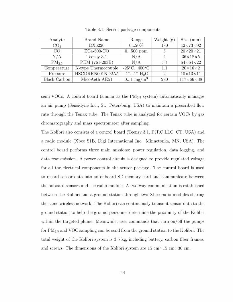
Table 3.1: Sensor package components
Analyte Brand Name Range Weight (g) Size (mm)CO2 DX6220 0...20% 180 42�73�92CO EC4-500-CO 0...500 ppm 5 20�20�21N/A Teensy 3.1 N/A 4 36�18�5
PM2.5 PEM (761-203B) N/A 53 64�64�22Temperature K-type Thermocouple -25�C...400�C 1.1 20�16�2
Pressure HSCDRRN001ND2A5 -1”...1” H2O 2 10�13�11Black Carbon MicoAeth AE51 0...1 mg/m3 280 117�66�38
semi-VOCs. A control board (similar as the PM2.5 system) automatically manages
an air pump (Sensidyne Inc., St. Petersburg, USA) to maintain a prescribed flow
rate through the Tenax tube. The Tenax tube is analyzed for certain VOCs by gas
chromatography and mass spectrometer after sampling.
The Kolibri also consists of a control board (Teensy 3.1, PJRC LLC, CT, USA) and
a radio module (Xbee S1B, Digi International Inc. Minnetonka, MN, USA). The
control board performs three main missions: power regulation, data logging, and
data transmission. A power control circuit is designed to provide regulated voltage
for all the electrical components in the sensor package. The control board is used
to record sensor data into an onboard SD memory card and communicate between
the onboard sensors and the radio module. A two-way communication is established
between the Kolibri and a ground station through two Xbee radio modules sharing
the same wireless network. The Kolibri can continuously transmit sensor data to the
ground station to help the ground personnel determine the proximity of the Kolibri
within the targeted plume. Meanwhile, user commands that turn on/off the pumps
for PM2.5 and VOC sampling can be send from the ground station to the Kolibri. The
total weight of the Kolibri system is 3.5 kg, including battery, carbon fiber frames,
and screws. The dimensions of the Kolibri system are 15 cm�15 cm�30 cm.
44
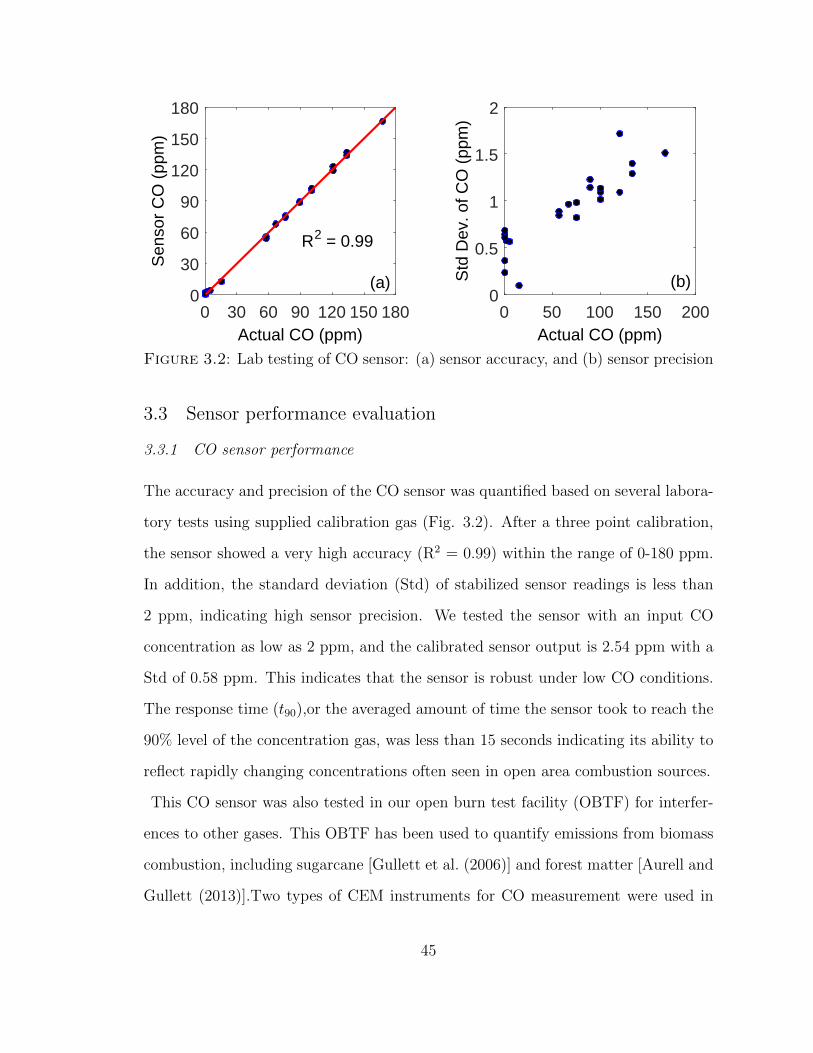
0 30 60 90 120 150 180Actual CO (ppm)
0
30
60
90
120
150
180
Sen
sor
CO
(pp
m)
0 50 100 150 200Actual CO (ppm)
0
0.5
1
1.5
2
Std
Dev
. of C
O (
ppm
)
R2 = 0.99
(b)(a)
Figure 3.2: Lab testing of CO sensor: (a) sensor accuracy, and (b) sensor precision
3.3 Sensor performance evaluation
3.3.1 CO sensor performance
The accuracy and precision of the CO sensor was quantified based on several labora-
tory tests using supplied calibration gas (Fig. 3.2). After a three point calibration,
the sensor showed a very high accuracy (R2 = 0.99) within the range of 0-180 ppm.
In addition, the standard deviation (Std) of stabilized sensor readings is less than
2 ppm, indicating high sensor precision. We tested the sensor with an input CO
concentration as low as 2 ppm, and the calibrated sensor output is 2.54 ppm with a
Std of 0.58 ppm. This indicates that the sensor is robust under low CO conditions.
The response time (t90),or the averaged amount of time the sensor took to reach the
90% level of the concentration gas, was less than 15 seconds indicating its ability to
reflect rapidly changing concentrations often seen in open area combustion sources.
This CO sensor was also tested in our open burn test facility (OBTF) for interfer-
ences to other gases. This OBTF has been used to quantify emissions from biomass
combustion, including sugarcane [Gullett et al. (2006)] and forest matter [Aurell and
Gullett (2013)].Two types of CEM instruments for CO measurement were used in
45
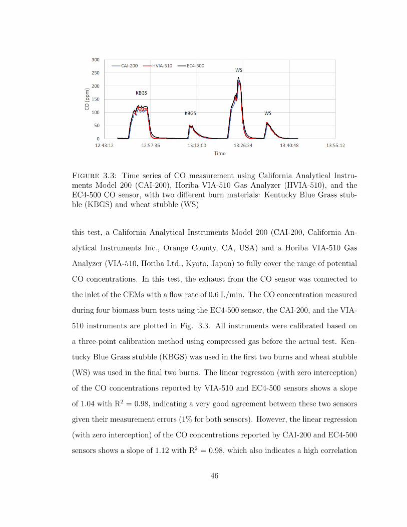
Figure 3.3: Time series of CO measurement using California Analytical Instru-ments Model 200 (CAI-200), Horiba VIA-510 Gas Analyzer (HVIA-510), and theEC4-500 CO sensor, with two different burn materials: Kentucky Blue Grass stub-ble (KBGS) and wheat stubble (WS)
this test, a California Analytical Instruments Model 200 (CAI-200, California An-
alytical Instruments Inc., Orange County, CA, USA) and a Horiba VIA-510 Gas
Analyzer (VIA-510, Horiba Ltd., Kyoto, Japan) to fully cover the range of potential
CO concentrations. In this test, the exhaust from the CO sensor was connected to
the inlet of the CEMs with a flow rate of 0.6 L/min. The CO concentration measured
during four biomass burn tests using the EC4-500 sensor, the CAI-200, and the VIA-
510 instruments are plotted in Fig. 3.3. All instruments were calibrated based on
a three-point calibration method using compressed gas before the actual test. Ken-
tucky Blue Grass stubble (KBGS) was used in the first two burns and wheat stubble
(WS) was used in the final two burns. The linear regression (with zero interception)
of the CO concentrations reported by VIA-510 and EC4-500 sensors shows a slope
of 1.04 with R2 = 0.98, indicating a very good agreement between these two sensors
given their measurement errors (1% for both sensors). However, the linear regression
(with zero interception) of the CO concentrations reported by CAI-200 and EC4-500
sensors shows a slope of 1.12 with R2 = 0.98, which also indicates a high correlation
46
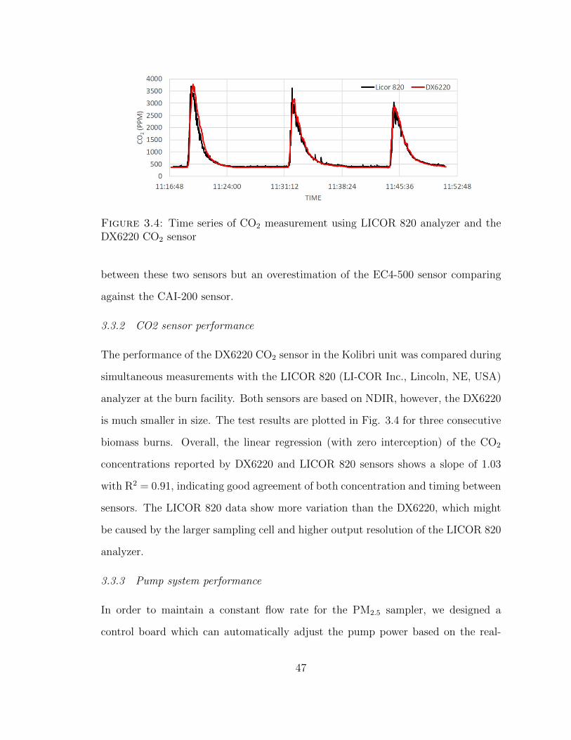
Figure 3.4: Time series of CO2 measurement using LICOR 820 analyzer and theDX6220 CO2 sensor
between these two sensors but an overestimation of the EC4-500 sensor comparing
against the CAI-200 sensor.
3.3.2 CO2 sensor performance
The performance of the DX6220 CO2 sensor in the Kolibri unit was compared during
simultaneous measurements with the LICOR 820 (LI-COR Inc., Lincoln, NE, USA)
analyzer at the burn facility. Both sensors are based on NDIR, however, the DX6220
is much smaller in size. The test results are plotted in Fig. 3.4 for three consecutive
biomass burns. Overall, the linear regression (with zero interception) of the CO2
concentrations reported by DX6220 and LICOR 820 sensors shows a slope of 1.03
with R2 = 0.91, indicating good agreement of both concentration and timing between
sensors. The LICOR 820 data show more variation than the DX6220, which might
be caused by the larger sampling cell and higher output resolution of the LICOR 820
analyzer.
3.3.3 Pump system performance
In order to maintain a constant flow rate for the PM2.5 sampler, we designed a
control board which can automatically adjust the pump power based on the real-
47
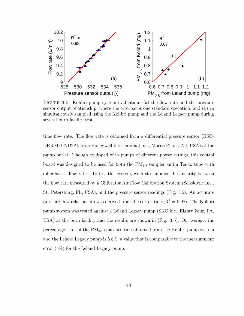
0.6 0.7 0.8 0.9 1 1.1 1.2PM
2.5 from Leland pump (mg)
0.6
0.7
0.8
0.9
1
1.1
1.2
PM
2.5 fr
om K
olib
ri (m
g)
528 530 532 534 536Pressure sensor output [-]
9
9.2
9.4
9.6
9.8
10
10.2
Flo
w r
ate
(L/m
in)
1:1
(a) (b)
R2 =0.87
R2 =0.98
Figure 3.5: Kolibri pump system evaluation: (a) the flow rate and the pressuresensor output relationship, where the errorbar is one standard deviation, and (b) 2.5
simultaneously sampled using the Kolibri pump and the Leland Legacy pump duringseveral burn facility tests
time flow rate. The flow rate is obtained from a differential pressure sensor (HSC-
DRRN001ND2A5 from Honeywell International Inc., Morris Plains, NJ, USA) at the
pump outlet. Though equipped with pumps of different power ratings, this control
board was designed to be used for both the PM2.5 sampler and a Tenax tube with
different set flow rates. To test this system, we first examined the linearity between
the flow rate measured by a Gilibrator Air Flow Calibration System (Sensidyne Inc.,
St. Petersburg, FL, USA), and the pressure sensor readings (Fig. 3.5). An accurate
pressure-flow relationship was derived from the correlation (R2 = 0.98). The Kolibri
pump system was tested against a Leland Legacy pump (SKC Inc., Eighty Four, PA,
USA) at the burn facility and the results are shown in (Fig. 3.5). On average, the
percentage error of the PM2.5 concentration obtained from the Kolibri pump system
and the Leland Legacy pump is 5.8%, a value that is comparable to the measurement
error (5%) for the Leland Legacy pump.
48
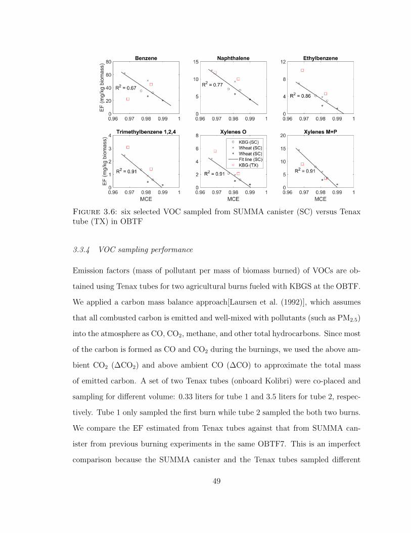
Figure 3.6: six selected VOC sampled from SUMMA canister (SC) versus Tenaxtube (TX) in OBTF
3.3.4 VOC sampling performance
Emission factors (mass of pollutant per mass of biomass burned) of VOCs are ob-
tained using Tenax tubes for two agricultural burns fueled with KBGS at the OBTF.
We applied a carbon mass balance approach[Laursen et al. (1992)], which assumes
that all combusted carbon is emitted and well-mixed with pollutants (such as PM2.5)
into the atmosphere as CO, CO2, methane, and other total hydrocarbons. Since most
of the carbon is formed as CO and CO2 during the burnings, we used the above am-
bient CO2 (∆CO2) and above ambient CO (∆CO) to approximate the total mass
of emitted carbon. A set of two Tenax tubes (onboard Kolibri) were co-placed and
sampling for different volume: 0.33 liters for tube 1 and 3.5 liters for tube 2, respec-
tively. Tube 1 only sampled the first burn while tube 2 sampled the both two burns.
We compare the EF estimated from Tenax tubes against that from SUMMA can-
ister from previous burning experiments in the same OBTF7. This is an imperfect
comparison because the SUMMA canister and the Tenax tubes sampled different
49
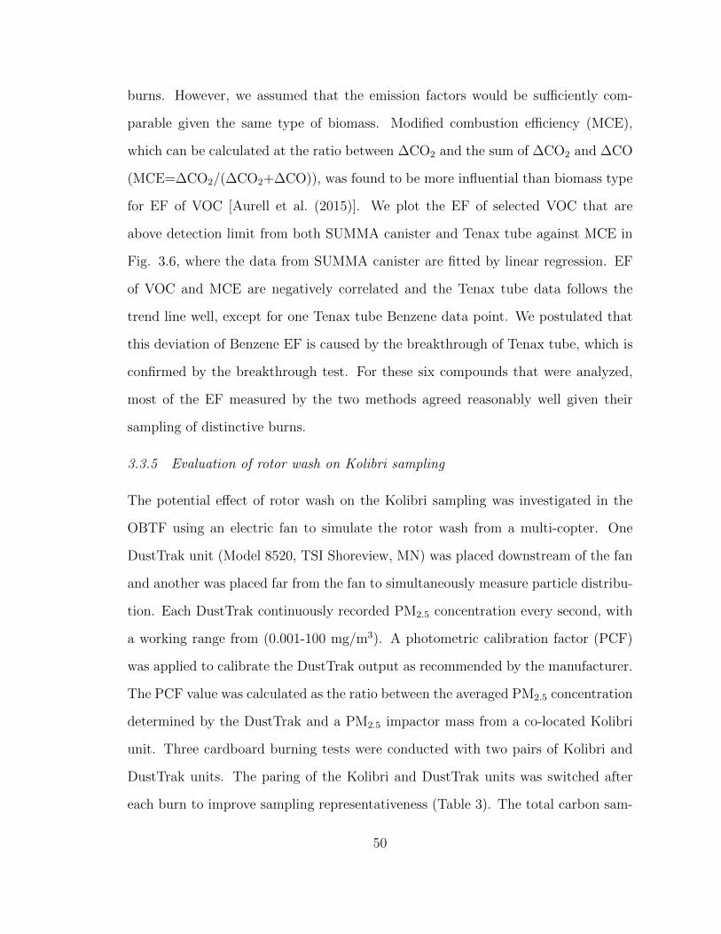
burns. However, we assumed that the emission factors would be sufficiently com-
parable given the same type of biomass. Modified combustion efficiency (MCE),
which can be calculated at the ratio between ∆CO2 and the sum of ∆CO2 and ∆CO
(MCE=∆CO2/(∆CO2+∆CO)), was found to be more influential than biomass type
for EF of VOC [Aurell et al. (2015)]. We plot the EF of selected VOC that are
above detection limit from both SUMMA canister and Tenax tube against MCE in
Fig. 3.6, where the data from SUMMA canister are fitted by linear regression. EF
of VOC and MCE are negatively correlated and the Tenax tube data follows the
trend line well, except for one Tenax tube Benzene data point. We postulated that
this deviation of Benzene EF is caused by the breakthrough of Tenax tube, which is
confirmed by the breakthrough test. For these six compounds that were analyzed,
most of the EF measured by the two methods agreed reasonably well given their
sampling of distinctive burns.
3.3.5 Evaluation of rotor wash on Kolibri sampling
The potential effect of rotor wash on the Kolibri sampling was investigated in the
OBTF using an electric fan to simulate the rotor wash from a multi-copter. One
DustTrak unit (Model 8520, TSI Shoreview, MN) was placed downstream of the fan
and another was placed far from the fan to simultaneously measure particle distribu-
tion. Each DustTrak continuously recorded PM2.5 concentration every second, with
a working range from (0.001-100 mg/m3). A photometric calibration factor (PCF)
was applied to calibrate the DustTrak output as recommended by the manufacturer.
The PCF value was calculated as the ratio between the averaged PM2.5 concentration
determined by the DustTrak and a PM2.5 impactor mass from a co-located Kolibri
unit. Three cardboard burning tests were conducted with two pairs of Kolibri and
DustTrak units. The paring of the Kolibri and DustTrak units was switched after
each burn to improve sampling representativeness (Table 3). The total carbon sam-
50
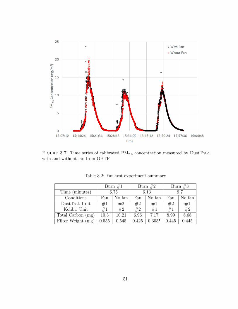
Figure 3.7: Time series of calibrated PM2.5 concentration measured by DustTrakwith and without fan from OBTF
Table 3.2: Fan test experiment summary
Burn #1 Burn #2 Burn #3Time (minutes) 6.75 6.13 9.7
Conditions Fan No fan Fan No fan Fan No fanDustTrak Unit #1 #2 #2 #1 #2 #1Kolibri Unit #1 #2 #2 #1 #1 #2
Total Carbon (mg) 10.3 10.21 6.96 7.17 8.99 8.68Filter Weight (mg) 0.555 0.545 0.425 0.305� 0.445 0.445
51
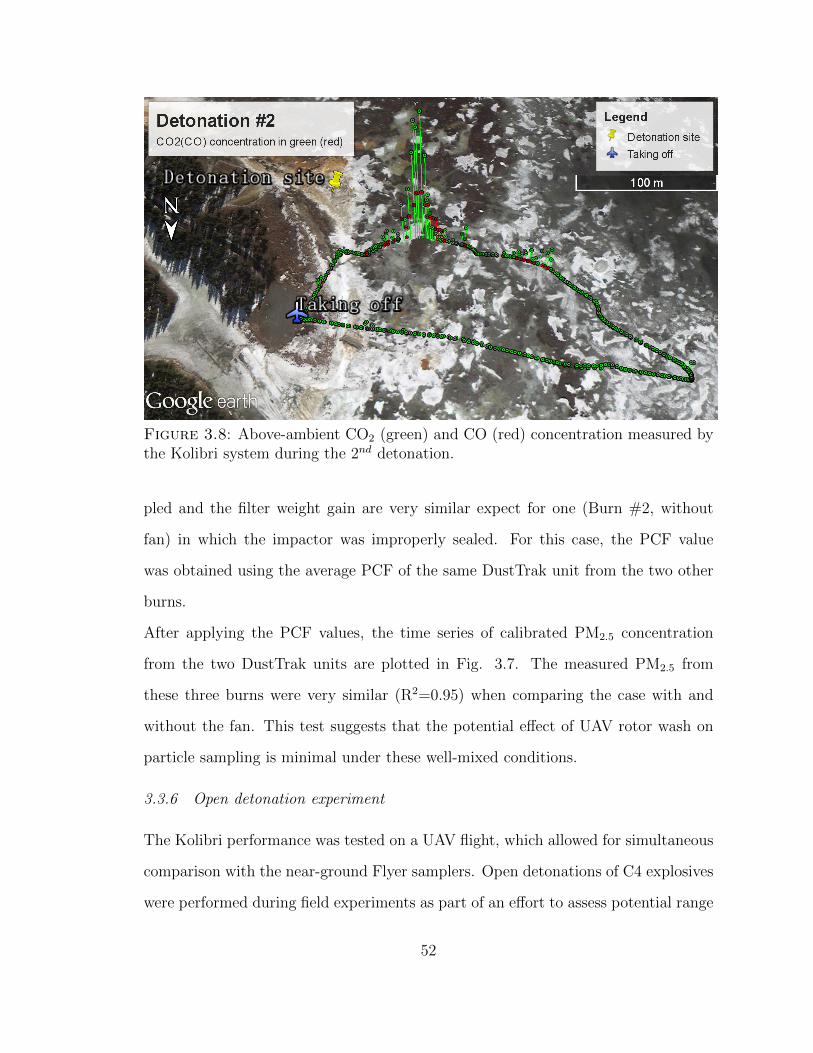
Figure 3.8: Above-ambient CO2 (green) and CO (red) concentration measured bythe Kolibri system during the 2nd detonation.
pled and the filter weight gain are very similar expect for one (Burn #2, without
fan) in which the impactor was improperly sealed. For this case, the PCF value
was obtained using the average PCF of the same DustTrak unit from the two other
burns.
After applying the PCF values, the time series of calibrated PM2.5 concentration
from the two DustTrak units are plotted in Fig. 3.7. The measured PM2.5 from
these three burns were very similar (R2=0.95) when comparing the case with and
without the fan. This test suggests that the potential effect of UAV rotor wash on
particle sampling is minimal under these well-mixed conditions.
3.3.6 Open detonation experiment
The Kolibri performance was tested on a UAV flight, which allowed for simultaneous
comparison with the near-ground Flyer samplers. Open detonations of C4 explosives
were performed during field experiments as part of an effort to assess potential range
52
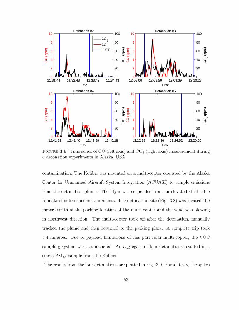
11:31:44 11:32:43 11:33:42 11:34:43Time
0
2
4
6
8
10
CO
(pp
m)
Detonation #2
11:31:44 11:32:43 11:33:42 11:34:430
20
40
60
80
100
CO
2 (
ppm
)
CO2
COPump
12:08:00 12:08:50 12:09:39 12:10:28Time
0
2
4
6
8
10
CO
(pp
m)
Detonation #3
12:08:00 12:08:50 12:09:39 12:10:280
20
40
60
80
100
CO
2 (
ppm
)
12:41:21 12:42:40 12:43:59 12:45:18Time
0
2
4
6
8
10
CO
(pp
m)
Detonation #4
12:41:21 12:42:40 12:43:59 12:45:180
20
40
60
80
100
CO
2 (
ppm
)
13:22:28 13:23:40 13:24:52 13:26:06Time
0
2
4
6
8
10
CO
(pp
m)
Detonation #5
13:22:28 13:23:40 13:24:52 13:26:060
20
40
60
80
100
CO
2 (
ppm
)
Figure 3.9: Time series of CO (left axis) and CO2 (right axis) measurement during4 detonation experiments in Alaska, USA
contamination. The Kolibri was mounted on a multi-copter operated by the Alaska
Center for Unmanned Aircraft System Integration (ACUASI) to sample emissions
from the detonation plume. The Flyer was suspended from an elevated steel cable
to make simultaneous measurements. The detonation site (Fig. 3.8) was located 100
meters south of the parking location of the multi-copter and the wind was blowing
in northwest direction. The multi-copter took off after the detonation, manually
tracked the plume and then returned to the parking place. A complete trip took
3-4 minutes. Due to payload limitations of this particular multi-copter, the VOC
sampling system was not included. An aggregate of four detonations resulted in a
single PM2.5 sample from the Kolibri.
The results from the four detonations are plotted in Fig. 3.9. For all tests, the spikes
53
of CO and CO2 concentration coincide with each other and indicate the times when
the Kolibri was successfully within the plume. Calculations of the carbon mass
using ∆CO2 and ∆CO when the Kolibri was sampling PM2.5 (pump on) enabled
determination of a PM2.5 emission factor of the C4 explosive from its carbon fraction
(0.2034). We obtained 39.4 mg PM2.5/gram C4 from the Kolibri system. A sensitivity
analysis performed using the errors from the CO (0.5 ppm) and CO2 (1% of readings)
sensors resulted in a PM2.5 emission factor ranging from 27.9 to 47.8 mg PM2.5/gram
C4. For comparison, the Flyer system reported 26.3 and 32.5 mg PM2.5/gram C4,
indicating comparable data from these limited tests.
3.4 Conclusion
A sensor/sampler system was designed and built for mobile and aerial emission sam-
pling. Both the CO and CO2 sensors show high accuracy, low noise, and quick
response. The PM2.5 sampler equipped with pump control system performed well
against a calibrated commercial pump. Emission factors of most VOCs sampled from
the Tenax tube show comparable results with previous SUMMA cannister sampling,
except in the case of volatile benzene which exhibits breakthrough. This system
is applicable to ground, ground-mobile, and aerial use. Its compact size and light
weight make it amenable for use on aerostats and UAVs. Trials of the system in
laboratory combustion tests and field applications sampling detonation plumes from
military explosives indicate that the system performs well and PM2.5 values are unaf-
fected by rotor wash under well-mixed conditions. The system can be readily applied
to a variety of open area emission scenarios with ground-based or airborne platforms
and can be modified to suit application-specific scenarios.
54
4
Fenceline Monitoring: A Bayesian Approach toLocating Fugitive Leaks
This chapter is based on the article: Zhou, X., Amaral, V., and Albertson, J. D.
Fenceline Monitoring: A Bayesian Approach to Locating Fugitive Leaks, under prepa-
ration
4.1 Introduction
Fugitive emissions from industrial facilities releases considerable amount of green-
house gases (GHG) and hazardous air pollutants (HAP) into the atmosphere. New
Source Performance Standards (NSPS) and National Emission Standards for Haz-
ardous Air Pollutants (NESHAP) regulates fugitive leaks from flanges/connectors,
valves, pumps, compressors, pressure relief devices, and agitators using Federal Ref-
erence Method 21 (FRM 21) suggested by United States Environmental Protection
Agency (USEPA). According to FRM 21, determination of emission compliance re-
quire exclusive inspection of all potential sources using specialized analyzers that is
labor-intensive and expensive depending on the scale of the facility. Also, this inspec-
55
tion is periodic thus emission between inspections are unknown. Average emission
factors are also been used to annual emissions of some pollutants based on installed
instruments and their operating conditions. However, this estimates have large un-
certainties and site-to-site variability can be high comparing against direct measure-
ments [Chambers et al. (2008); Allen et al. (2013)].
Various new monitoring techniques and source detection algorithms are available in
the literature. Brereton and Johnson (2012) applied a trajectory statistical methods
(TSM) to trace large leak source locations in complex refinery domains. However,
this method cannot determine leak rates effectively, which is equally important in
prioritizing the remediation of leaks given limited resources. Thoma et al. (2011)
tested the usage of 2-week passive sampler network in Corpus Christi, TX dur-
ing a year-long field study and the results are promising. Humphries et al. (2012)
used a network of sensors and successfully identified the location and release rate
of a controlled leak surrounded by the sensors based on Bayesian inference. Using
a similar Bayesian inference model, Yee (2007) proposed a Markov Chain Monte
Carlo (MCMC) method to estimate multiple leak. Recently, the USEPA issued a
updated the national emission standard for HAP that would require petroleum re-
fineries to continuously monitor along the fenceline of refinery facilities using passive
tube samplers at a two-weeks sampling frequency [U.S. Environmental Protection
Agency (EPA) (2015b)]. This newly proposed rule also reviewed other sensor tech-
nology for long-term fenceline monitoring [U.S. Environmental Protection Agency
(EPA) (2015b)]: active daily monitoring sensor networks, ”open-path” sensors based
on spectrum analysis in ultraviolet (UV-DOAS), and open-path sensors based on
spectrum analysis in infrared (FTIR). The emergence of low-cost sensors provides
another possibility for fenceline monitoring. Though this type of sensor usually has
a narrow detectable range, considerable sensor noise, and slow response, its low price
allows for a much denser sensor network which can potentially compensate for the
56
undesirable sensor performance.
As a first step, this paper seeks to evaluate the trade-off between sensor quality and
quantity of different fenceline monitoring methods for leak detection. Since the devel-
opment of sensor industry allows rapid improvement of sensor quality and application
of new sensing technology, the evaluation a specific sensor can be outdated soon. In-
stead, we focus on “idealized” sensors with different sensing mechanism and qualities
in this study. According to U.S. Environmental Protection Agency (EPA) (2015b),
we categorize the candidate sensors for fenceline monitoring into three main types:
point-scale real-time sensors, point-scale time-integrated sensors, and line-averaged
real-time sensors. The 2-week passive tube samplers and active daily monitoring sen-
sors can be grouped as point-scale time-integrated sensors with different sampling
frequency. Both the UV-DOAS and the FTIR ”open-path” sensors can be classified
as line-averaged real-time sensors. There is a large amount of point-scale real-time
sensors available in the market with varying quality and sensing mechanism, such
as the photoionization sensors, cavity ring down spectroscopy, and open-path CH4
analyzer. For a given monitoring method, its “skill” of leak detection is a function
of sensor quantity and quality of the chosen sensor.
For a simple reference comparison, we consider an imaginary domain with one con-
tinuous leak and evenly distributed sensors on the domain edge. First, a disper-
sion model is used to simulate concentration field from the emitting leak driven by
prescribed wind data. Then, a sensor reception model is formulated to estimate
sensor-measured concentration as a function of actual gas concentration and sensor
characteristics such as sensor type, sensor error, and sampling duration. Finally,
a Bayesian inference model is utilized to identify location and emission rate of the
leak based on the sensor-measured concentration. Bayesian inference has been used
extensively for leak detection largely due to its concrete mechanism of combining
the evidence with prior knowledge, easily interpretable probabilistic result, and con-
57
venient compliance with other models. We use errors of leak localization and rate
estimation to evaluate the performance of different fenceline monitoring techniques,
which is also a function of sensor quality and quantity. Results show that different
sensing methods have their own strength and weakness based on possible source of
errors. More importantly, we found that a dense network can always provide faster
estimations, and can compensate for some sensor inferiority such as sensor noise and
produce similar or even superior leak-identification ability compare against sparse
sensor network. Though idealized, this result shows promise of applying low-cost,
point-scale sensor networks for fenceline monitoring.
4.2 Method
Here we describe the scheme of the Bayesian inference from fenceline monitoring mea-
surements Fig. 4.1. Consider a real-world leak scenario with a continuous and steady
leak located at x0 emitting at a rate of Q0. The leak will generate a elevated concen-
tration field CDP0 pxq|I0 based on the actual landscape and meteorological conditions
I0 such as wind speed, wind direction, surface roughness and atmospheric stability
conditions. The leak is surround by several fenceline sensors location at (xk) they will
output a signal of CSP0 pxkq according to its sensor characteristics, such as sampling
frequency, detection limit. The Bayesian inference model is aim to identify the leak
location x0 and its leak rate Q0 based on the measured concentration CSP0 pxkq and
our knowledge of plume dispersion, sensor characteristics, and possible errors. To do
so, we first model a concentration field, CDMi,j pxq|I, generated from a leak located at
xi with emission rate of Qj based on measured landscape and meteorological condi-
tions I. It should be noted the modeled concentration field may differ from the actual
one even if the leak location and leak rate are the same. This can be attributed to
the error of the dispersion model in representing the actual physical process of plume
transport and mixing, and the mismatch between the actual (I0) and measured (I)
58
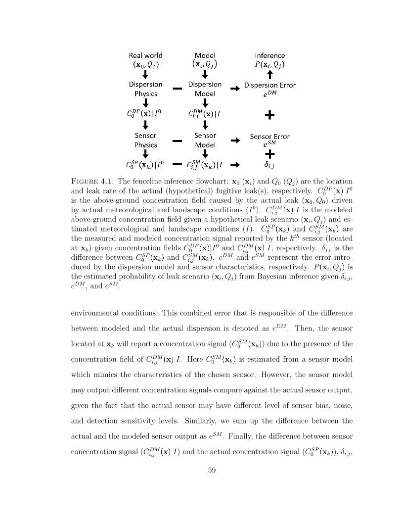
Figure 4.1: The fenceline inference flowchart: x0 (xi) and Q0 (Qj) are the locationand leak rate of the actual (hypothetical) fugitive leak(s), respectively. CDP
0 pxq|I0
is the above-ground concentration field caused by the actual leak (x0, Q0) drivenby actual meteorological and landscape conditions (I0). CDM
i,j pxq|I is the modeledabove-ground concentration field given a hypothetical leak scenario (xi, Qj) and es-timated meteorological and landscape conditions (I). CSP
0 pxkq and CSMi,j pxkq are
the measured and modeled concentration signal reported by the kth sensor (locatedat xk) given concentration fields CDP
0 pxq|I0 and CDMi,j pxq|I, respectively. δj,i is the
difference between CSP0 pxkq and CSM
i,j pxkq. eDM and eSM represent the error intro-duced by the dispersion model and sensor characteristics, respectively. P pxi, Qjq isthe estimated probability of leak scenario (xi, Qj) from Bayesian inference given δi,j,eDM , and eSM .
environmental conditions. This combined error that is responsible of the difference
between modeled and the actual dispersion is denoted as eDM . Then, the sensor
located at xk will report a concentration signal (CSM0 pxkq) due to the presence of the
concentration field of CDMi,j pxq|I. Here CSM
0 pxkq is estimated from a sensor model
which mimics the characteristics of the chosen sensor. However, the sensor model
may output different concentration signals compare against the actual sensor output,
given the fact that the actual sensor may have different level of sensor bias, noise,
and detection sensitivity levels. Similarly, we sum up the difference between the
actual and the modeled sensor output as eSM . Finally, the difference between sensor
concentration signal (CDMi,j pxq|I) and the actual concentration signal (CSP
0 pxkq), δi,j,
59
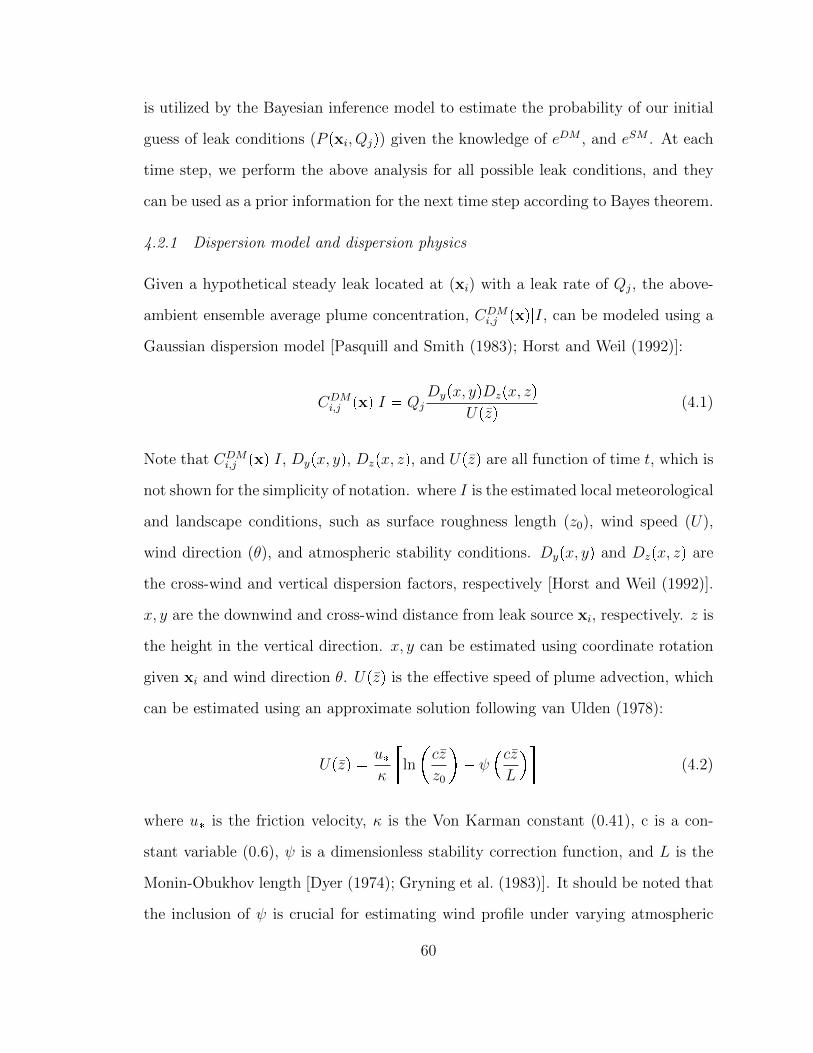
is utilized by the Bayesian inference model to estimate the probability of our initial
guess of leak conditions (P pxi, Qjq) given the knowledge of eDM , and eSM . At each
time step, we perform the above analysis for all possible leak conditions, and they
can be used as a prior information for the next time step according to Bayes theorem.
4.2.1 Dispersion model and dispersion physics
Given a hypothetical steady leak located at (xi) with a leak rate of Qj, the above-
ambient ensemble average plume concentration, CDMi,j pxq|I, can be modeled using a
Gaussian dispersion model [Pasquill and Smith (1983); Horst and Weil (1992)]:
CDMi,j pxq|I � Qj
Dypx, yqDzpx, zqUpzq (4.1)
Note that CDMi,j pxq|I, Dypx, yq, Dzpx, zq, and Upzq are all function of time t, which is
not shown for the simplicity of notation. where I is the estimated local meteorological
and landscape conditions, such as surface roughness length (z0), wind speed (U),
wind direction (θ), and atmospheric stability conditions. Dypx, yq and Dzpx, zq are
the cross-wind and vertical dispersion factors, respectively [Horst and Weil (1992)].
x, y are the downwind and cross-wind distance from leak source xi, respectively. z is
the height in the vertical direction. x, y can be estimated using coordinate rotation
given xi and wind direction θ. Upzq is the effective speed of plume advection, which
can be estimated using an approximate solution following van Ulden (1978):
Upzq � u�κ
�ln
�cz
z0
� ψ
�czL
�(4.2)
where u� is the friction velocity, κ is the Von Karman constant (0.41), c is a con-
stant variable (0.6), ψ is a dimensionless stability correction function, and L is the
Monin-Obukhov length [Dyer (1974); Gryning et al. (1983)]. It should be noted that
the inclusion of ψ is crucial for estimating wind profile under varying atmospheric
60
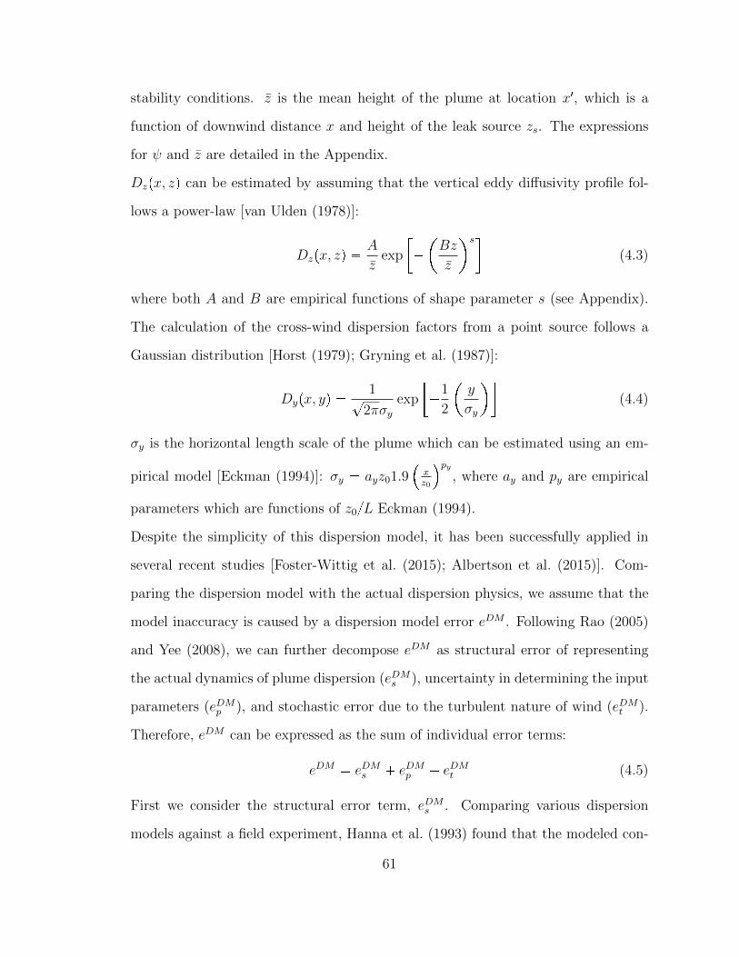
stability conditions. z is the mean height of the plume at location x1, which is a
function of downwind distance x and height of the leak source zs. The expressions
for ψ and z are detailed in the Appendix.
Dzpx, zq can be estimated by assuming that the vertical eddy diffusivity profile fol-
lows a power-law [van Ulden (1978)]:
Dzpx, zq � A
zexp
���Bz
z
s�(4.3)
where both A and B are empirical functions of shape parameter s (see Appendix).
The calculation of the cross-wind dispersion factors from a point source follows a
Gaussian distribution [Horst (1979); Gryning et al. (1987)]:
Dypx, yq � 1?2πσy
exp
��1
2
�y
σy
�(4.4)
σy is the horizontal length scale of the plume which can be estimated using an em-
pirical model [Eckman (1994)]: σy � ayz01.9�xz0
py, where ay and py are empirical
parameters which are functions of z0{L Eckman (1994).
Despite the simplicity of this dispersion model, it has been successfully applied in
several recent studies [Foster-Wittig et al. (2015); Albertson et al. (2015)]. Com-
paring the dispersion model with the actual dispersion physics, we assume that the
model inaccuracy is caused by a dispersion model error eDM . Following Rao (2005)
and Yee (2008), we can further decompose eDM as structural error of representing
the actual dynamics of plume dispersion (eDMs ), uncertainty in determining the input
parameters (eDMp ), and stochastic error due to the turbulent nature of wind (eDMt ).
Therefore, eDM can be expressed as the sum of individual error terms:
eDM � eDMs � eDMp � eDMt (4.5)
First we consider the structural error term, eDMs . Comparing various dispersion
models against a field experiment, Hanna et al. (1993) found that the modeled con-
61
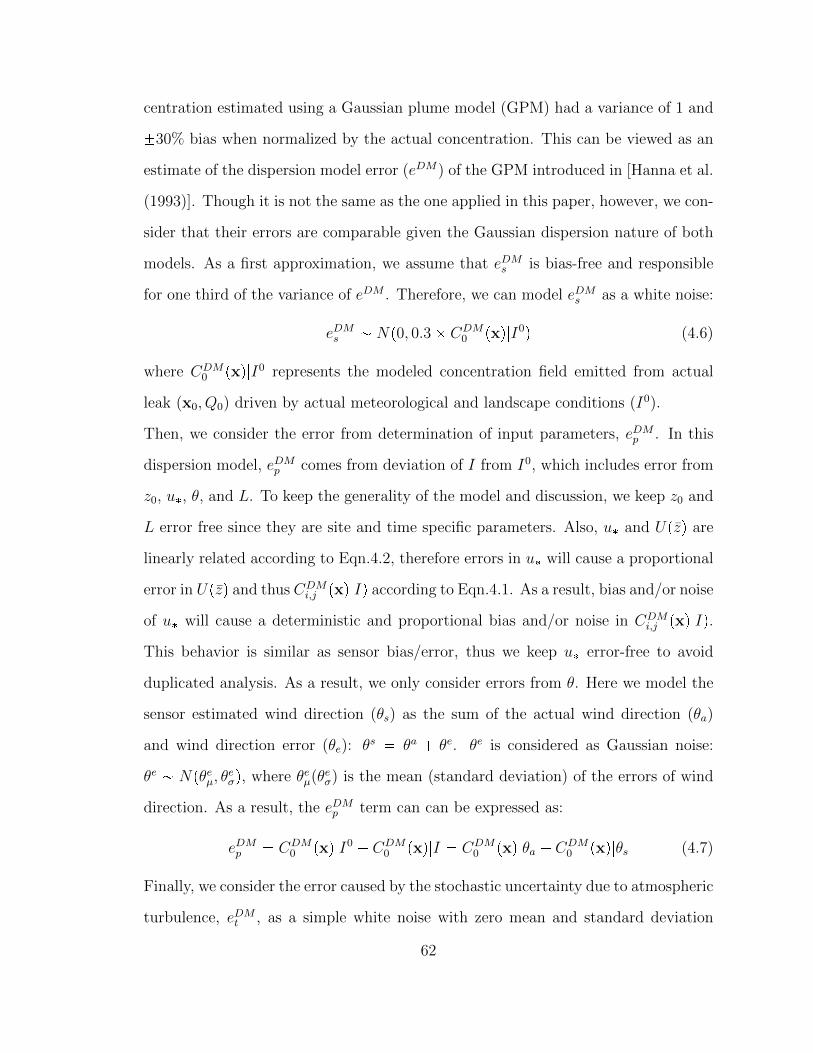
centration estimated using a Gaussian plume model (GPM) had a variance of 1 and
�30% bias when normalized by the actual concentration. This can be viewed as an
estimate of the dispersion model error (eDM) of the GPM introduced in [Hanna et al.
(1993)]. Though it is not the same as the one applied in this paper, however, we con-
sider that their errors are comparable given the Gaussian dispersion nature of both
models. As a first approximation, we assume that eDMs is bias-free and responsible
for one third of the variance of eDM . Therefore, we can model eDMs as a white noise:
eDMs � Np0, 0.3 � CDM0 pxq|I0q (4.6)
where CDM0 pxq|I0 represents the modeled concentration field emitted from actual
leak (x0, Q0) driven by actual meteorological and landscape conditions (I0).
Then, we consider the error from determination of input parameters, eDMp . In this
dispersion model, eDMp comes from deviation of I from I0, which includes error from
z0, u�, θ, and L. To keep the generality of the model and discussion, we keep z0 and
L error free since they are site and time specific parameters. Also, u� and Upzq are
linearly related according to Eqn.4.2, therefore errors in u� will cause a proportional
error in Upzq and thus CDMi,j pxq|Iq according to Eqn.4.1. As a result, bias and/or noise
of u� will cause a deterministic and proportional bias and/or noise in CDMi,j pxq|Iq.
This behavior is similar as sensor bias/error, thus we keep u� error-free to avoid
duplicated analysis. As a result, we only consider errors from θ. Here we model the
sensor estimated wind direction (θs) as the sum of the actual wind direction (θa)
and wind direction error (θe): θs � θa � θe. θe is considered as Gaussian noise:
θe � Npθeµ, θeσq, where θeµ(θeσ) is the mean (standard deviation) of the errors of wind
direction. As a result, the eDMp term can can be expressed as:
eDMp � CDM0 pxq|I0 � CDM
0 pxq|I � CDM0 pxq|θa � CDM
0 pxq|θs (4.7)
Finally, we consider the error caused by the stochastic uncertainty due to atmospheric
turbulence, eDMt , as a simple white noise with zero mean and standard deviation
62
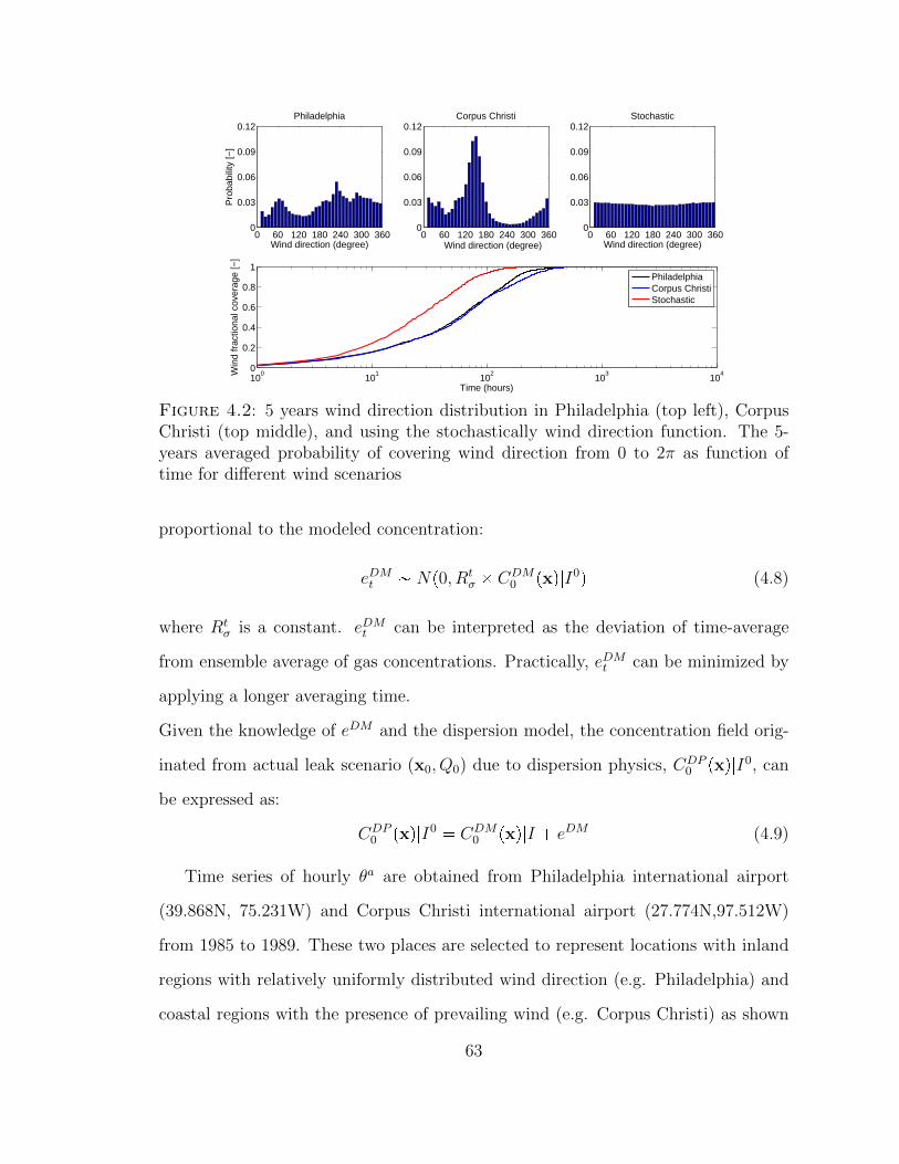
0 60 120 180 240 300 3600
0.03
0.06
0.09
0.12Stochastic
Wind direction (degree)
100
101
102
103
104
0
0.2
0.4
0.6
0.8
1
Time (hours)
Win
d fr
actio
nal c
over
age
[−]
0 60 120 180 240 300 3600
0.03
0.06
0.09
0.12Philadelphia
Wind direction (degree)
Pro
babi
lity
[−]
0 60 120 180 240 300 3600
0.03
0.06
0.09
0.12Corpus Christi
Wind direction (degree)
PhiladelphiaCorpus ChristiStochastic
Figure 4.2: 5 years wind direction distribution in Philadelphia (top left), CorpusChristi (top middle), and using the stochastically wind direction function. The 5-years averaged probability of covering wind direction from 0 to 2π as function oftime for different wind scenarios
proportional to the modeled concentration:
eDMt � Np0, Rtσ � CDM
0 pxq|I0q (4.8)
where Rtσ is a constant. eDMt can be interpreted as the deviation of time-average
from ensemble average of gas concentrations. Practically, eDMt can be minimized by
applying a longer averaging time.
Given the knowledge of eDM and the dispersion model, the concentration field orig-
inated from actual leak scenario (x0, Q0) due to dispersion physics, CDP0 pxq|I0, can
be expressed as:
CDP0 pxq|I0 � CDM
0 pxq|I � eDM (4.9)
Time series of hourly θa are obtained from Philadelphia international airport
(39.868N, 75.231W) and Corpus Christi international airport (27.774N,97.512W)
from 1985 to 1989. These two places are selected to represent locations with inland
regions with relatively uniformly distributed wind direction (e.g. Philadelphia) and
coastal regions with the presence of prevailing wind (e.g. Corpus Christi) as shown
63
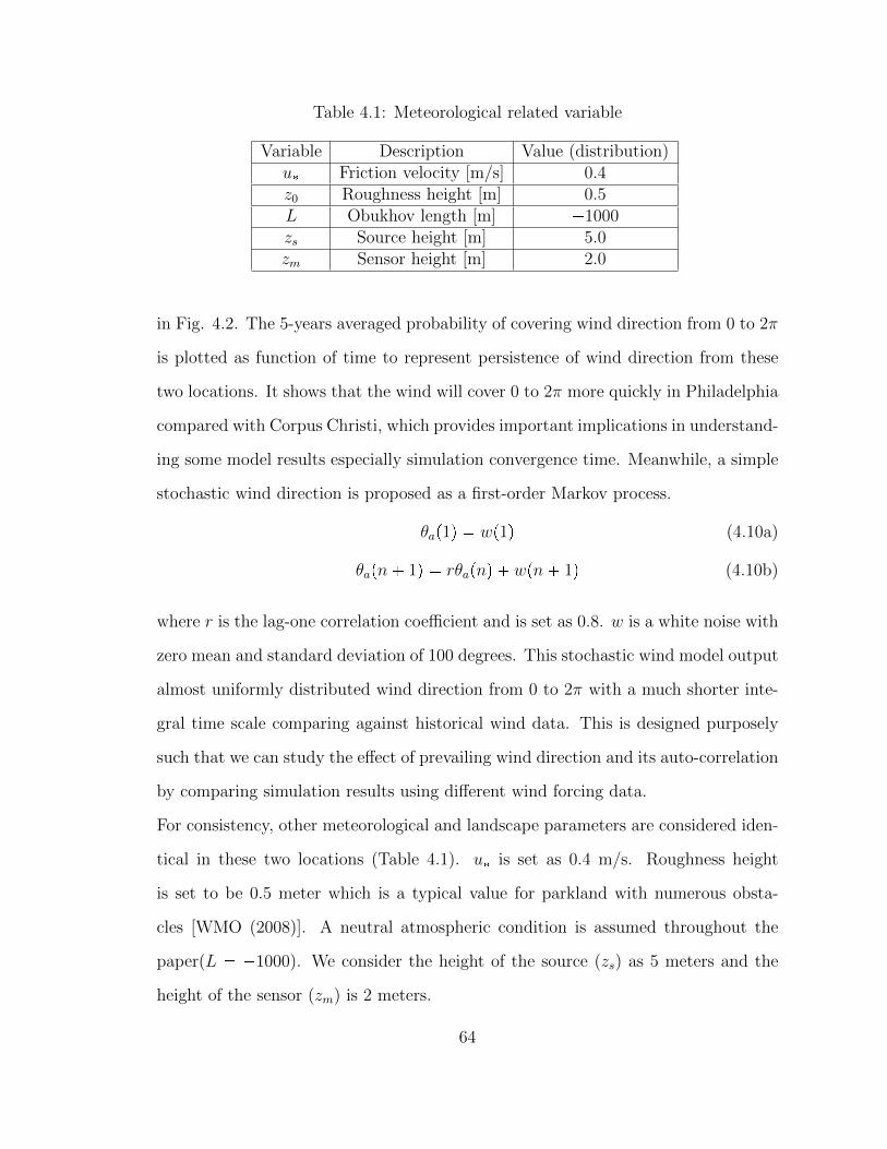
Table 4.1: Meteorological related variable
Variable Description Value (distribution)u� Friction velocity [m/s] 0.4z0 Roughness height [m] 0.5L Obukhov length [m] �1000zs Source height [m] 5.0zm Sensor height [m] 2.0
in Fig. 4.2. The 5-years averaged probability of covering wind direction from 0 to 2π
is plotted as function of time to represent persistence of wind direction from these
two locations. It shows that the wind will cover 0 to 2π more quickly in Philadelphia
compared with Corpus Christi, which provides important implications in understand-
ing some model results especially simulation convergence time. Meanwhile, a simple
stochastic wind direction is proposed as a first-order Markov process.
θap1q � wp1q (4.10a)
θapn� 1q � rθapnq � wpn� 1q (4.10b)
where r is the lag-one correlation coefficient and is set as 0.8. w is a white noise with
zero mean and standard deviation of 100 degrees. This stochastic wind model output
almost uniformly distributed wind direction from 0 to 2π with a much shorter inte-
gral time scale comparing against historical wind data. This is designed purposely
such that we can study the effect of prevailing wind direction and its auto-correlation
by comparing simulation results using different wind forcing data.
For consistency, other meteorological and landscape parameters are considered iden-
tical in these two locations (Table 4.1). u� is set as 0.4 m/s. Roughness height
is set to be 0.5 meter which is a typical value for parkland with numerous obsta-
cles [WMO (2008)]. A neutral atmospheric condition is assumed throughout the
paper(L � �1000). We consider the height of the source (zs) as 5 meters and the
height of the sensor (zm) is 2 meters.
64
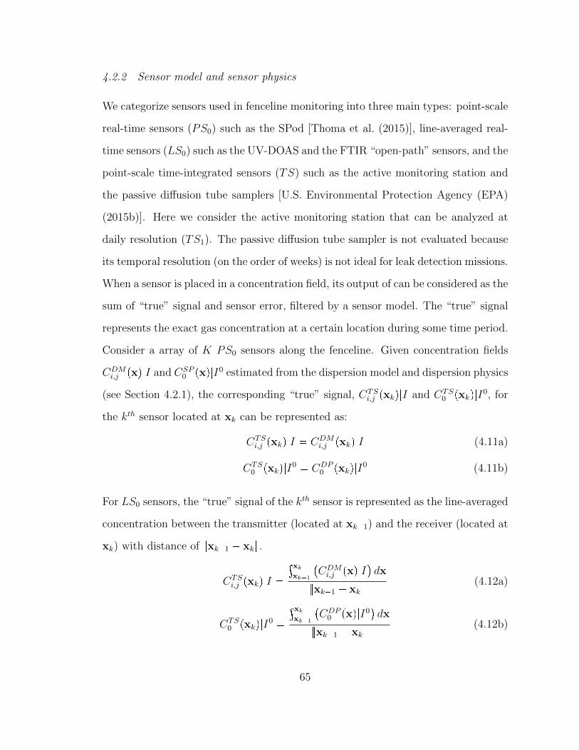
4.2.2 Sensor model and sensor physics
We categorize sensors used in fenceline monitoring into three main types: point-scale
real-time sensors (PS0) such as the SPod [Thoma et al. (2015)], line-averaged real-
time sensors (LS0) such as the UV-DOAS and the FTIR “open-path” sensors, and the
point-scale time-integrated sensors (TS) such as the active monitoring station and
the passive diffusion tube samplers [U.S. Environmental Protection Agency (EPA)
(2015b)]. Here we consider the active monitoring station that can be analyzed at
daily resolution (TS1). The passive diffusion tube sampler is not evaluated because
its temporal resolution (on the order of weeks) is not ideal for leak detection missions.
When a sensor is placed in a concentration field, its output of can be considered as the
sum of “true” signal and sensor error, filtered by a sensor model. The “true” signal
represents the exact gas concentration at a certain location during some time period.
Consider a array of K PS0 sensors along the fenceline. Given concentration fields
CDMi,j pxq|I and CSP
0 pxq|I0 estimated from the dispersion model and dispersion physics
(see Section 4.2.1), the corresponding “true” signal, CTSi,j pxkq|I and CTS
0 pxkq|I0, for
the kth sensor located at xk can be represented as:
CTSi,j pxkq|I � CDM
i,j pxkq|I (4.11a)
CTS0 pxkq|I0 � CDP
0 pxkq|I0 (4.11b)
For LS0 sensors, the “true” signal of the kth sensor is represented as the line-averaged
concentration between the transmitter (located at xk�1) and the receiver (located at
xk) with distance of }xk�1 � xk}.
CTSi,j pxkq|I �
³xk
xk�1
�CDMi,j pxq|I� dx
}xk�1 � xk} (4.12a)
CTS0 pxkq|I0 �
³xk
xk�1
�CDP
0 pxq|I0�dx
}xk�1 � xk} (4.12b)
65
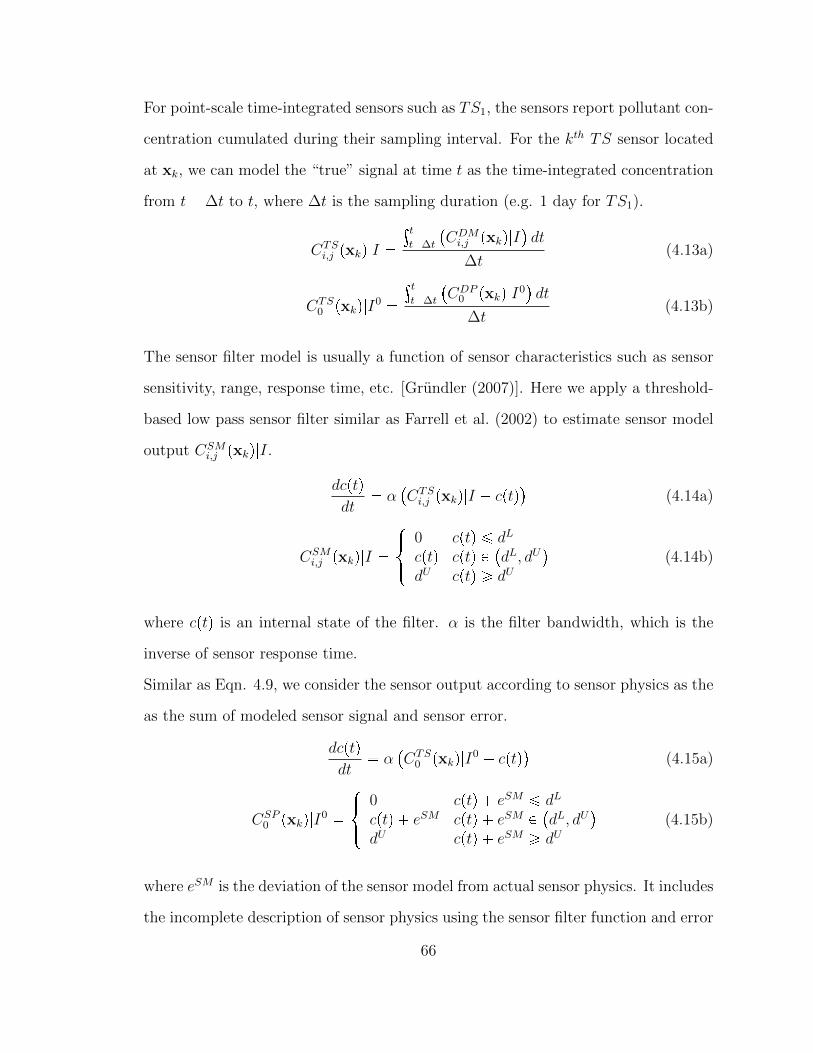
For point-scale time-integrated sensors such as TS1, the sensors report pollutant con-
centration cumulated during their sampling interval. For the kth TS sensor located
at xk, we can model the “true” signal at time t as the time-integrated concentration
from t� ∆t to t, where ∆t is the sampling duration (e.g. 1 day for TS1).
CTSi,j pxkq|I �
³tt�∆t
�CDMi,j pxkq|I
�dt
∆t(4.13a)
CTS0 pxkq|I0 �
³tt�∆t
�CDP
0 pxkq|I0�dt
∆t(4.13b)
The sensor filter model is usually a function of sensor characteristics such as sensor
sensitivity, range, response time, etc. [Grundler (2007)]. Here we apply a threshold-
based low pass sensor filter similar as Farrell et al. (2002) to estimate sensor model
output CSMi,j pxkq|I.
dcptqdt
� α�CTSi,j pxkq|I � cptq� (4.14a)
CSMi,j pxkq|I �
$&%
0 cptq ¤ dL
cptq cptq P �dL, dU�dU cptq ¥ dU
(4.14b)
where cptq is an internal state of the filter. α is the filter bandwidth, which is the
inverse of sensor response time.
Similar as Eqn. 4.9, we consider the sensor output according to sensor physics as the
as the sum of modeled sensor signal and sensor error.
dcptqdt
� α�CTS
0 pxkq|I0 � cptq� (4.15a)
CSP0 pxkq|I0 �
$&%
0 cptq � eSM ¤ dL
cptq � eSM cptq � eSM P �dL, dU�dU cptq � eSM ¥ dU
(4.15b)
where eSM is the deviation of the sensor model from actual sensor physics. It includes
the incomplete description of sensor physics using the sensor filter function and error
66
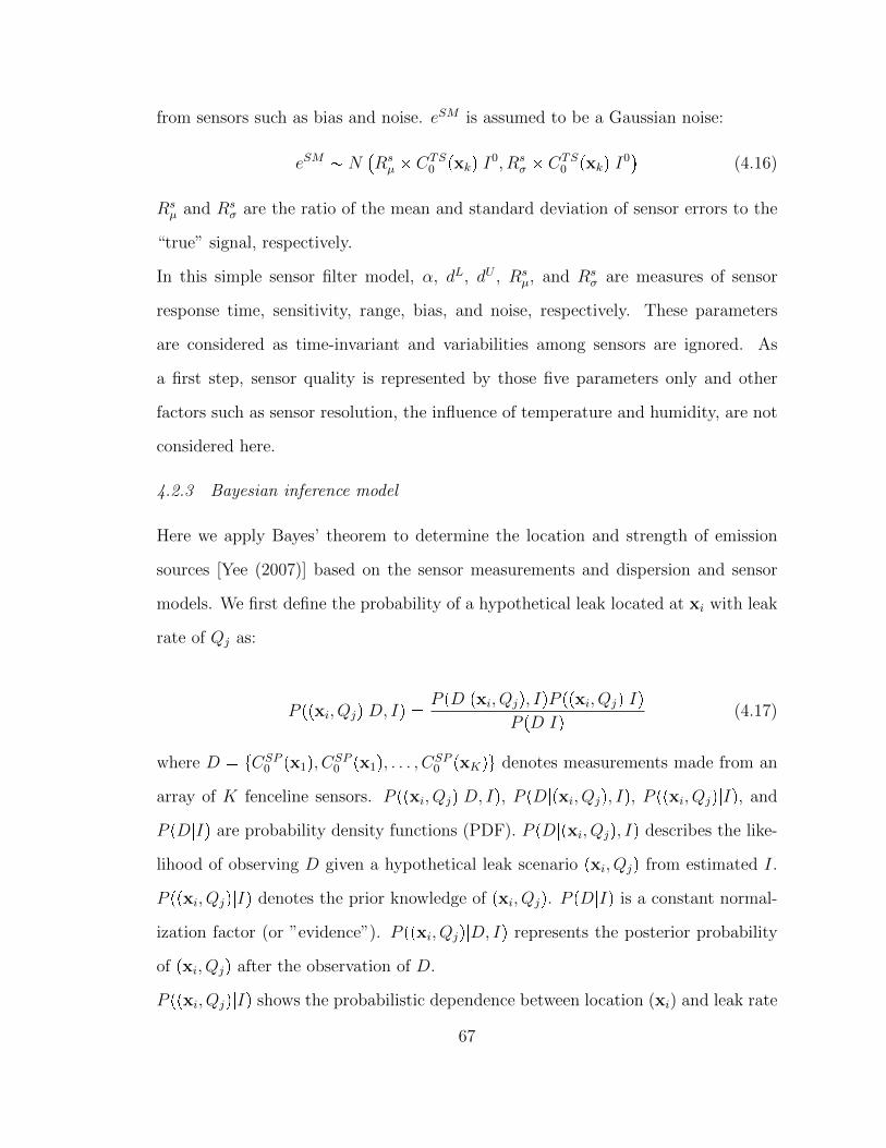
from sensors such as bias and noise. eSM is assumed to be a Gaussian noise:
eSM � N�Rsµ � CTS
0 pxkq|I0, Rsσ � CTS
0 pxkq|I0�
(4.16)
Rsµ and Rs
σ are the ratio of the mean and standard deviation of sensor errors to the
“true” signal, respectively.
In this simple sensor filter model, α, dL, dU , Rsµ, and Rs
σ are measures of sensor
response time, sensitivity, range, bias, and noise, respectively. These parameters
are considered as time-invariant and variabilities among sensors are ignored. As
a first step, sensor quality is represented by those five parameters only and other
factors such as sensor resolution, the influence of temperature and humidity, are not
considered here.
4.2.3 Bayesian inference model
Here we apply Bayes’ theorem to determine the location and strength of emission
sources [Yee (2007)] based on the sensor measurements and dispersion and sensor
models. We first define the probability of a hypothetical leak located at xi with leak
rate of Qj as:
P ppxi, Qjq|D, Iq � P pD|pxi, Qjq, IqP ppxi, Qjq|IqP pD|Iq (4.17)
where D � tCSP0 px1q, CSP
0 px1q, . . . , CSP0 pxKqu denotes measurements made from an
array of K fenceline sensors. P ppxi, Qjq|D, Iq, P pD|pxi, Qjq, Iq, P ppxi, Qjq|Iq, and
P pD|Iq are probability density functions (PDF). P pD|pxi, Qjq, Iq describes the like-
lihood of observing D given a hypothetical leak scenario pxi, Qjq from estimated I.
P ppxi, Qjq|Iq denotes the prior knowledge of pxi, Qjq. P pD|Iq is a constant normal-
ization factor (or ”evidence”). P ppxi, Qjq|D, Iq represents the posterior probability
of pxi, Qjq after the observation of D.
P ppxi, Qjq|Iq shows the probabilistic dependence between location (xi) and leak rate
67
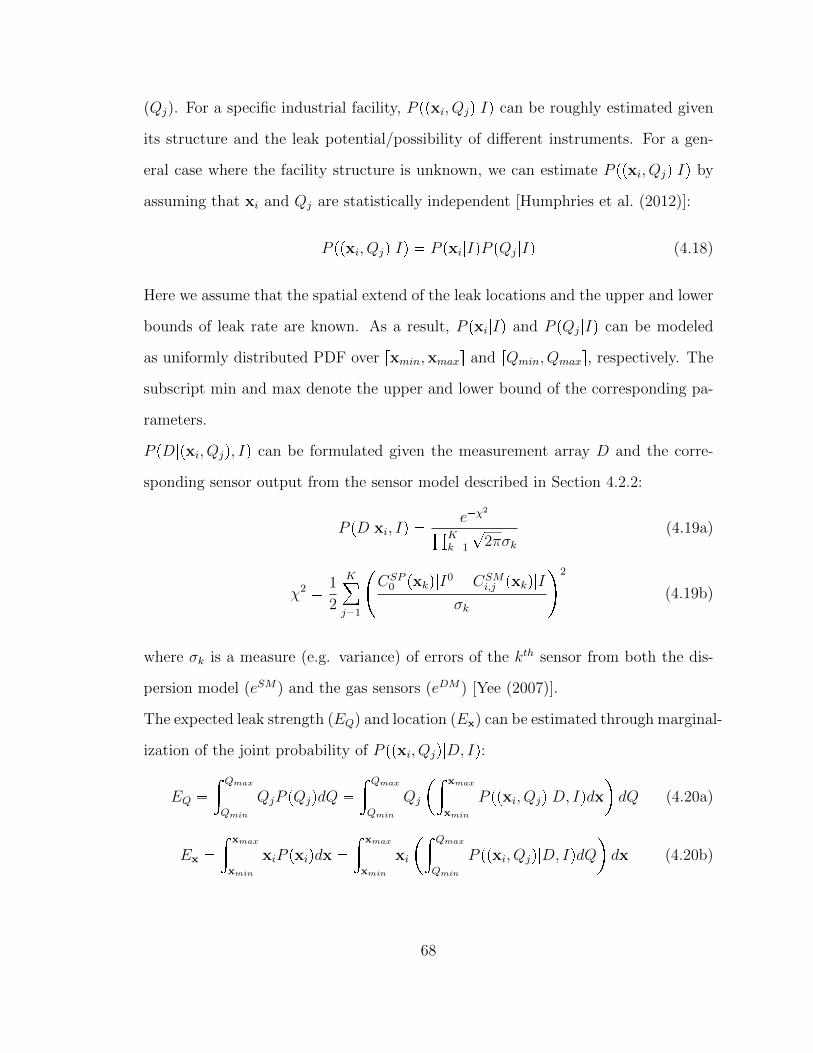
(Qj). For a specific industrial facility, P ppxi, Qjq|Iq can be roughly estimated given
its structure and the leak potential/possibility of different instruments. For a gen-
eral case where the facility structure is unknown, we can estimate P ppxi, Qjq|Iq by
assuming that xi and Qj are statistically independent [Humphries et al. (2012)]:
P ppxi, Qjq|Iq � P pxi|IqP pQj|Iq (4.18)
Here we assume that the spatial extend of the leak locations and the upper and lower
bounds of leak rate are known. As a result, P pxi|Iq and P pQj|Iq can be modeled
as uniformly distributed PDF over rxmin,xmaxs and rQmin, Qmaxs, respectively. The
subscript min and max denote the upper and lower bound of the corresponding pa-
rameters.
P pD|pxi, Qjq, Iq can be formulated given the measurement array D and the corre-
sponding sensor output from the sensor model described in Section 4.2.2:
P pD|xi, Iq � e�χ2±K
k�1
?2πσk
(4.19a)
χ2 � 1
2
K
j�1
�CSP
0 pxkq|I0 � CSMi,j pxkq|I
σk
�2
(4.19b)
where σk is a measure (e.g. variance) of errors of the kth sensor from both the dis-
persion model (eSM) and the gas sensors (eDM) [Yee (2007)].
The expected leak strength (EQ) and location (Ex) can be estimated through marginal-
ization of the joint probability of P ppxi, Qjq|D, Iq:
EQ �» Qmax
Qmin
QjP pQjqdQ �» Qmax
Qmin
Qj
�» xmax
xmin
P ppxi, Qjq|D, IqdxdQ (4.20a)
Ex �» xmax
xmin
xiP pxiqdx �» xmax
xmin
xi
�» Qmax
Qmin
P ppxi, Qjq|D, IqdQdx (4.20b)
68
Figure 4.3: A cartoon of the computational domain containing rectangular gridcells with a size of ∆x�∆y. Each grid cell (e.g. xi) is treated as a hypothetical leaklocation with leak rate Qj, which is detonated by an open circle. The actual leaklocated at x0 with leak rate of Q0 is shown as a solid circle. Sensors (solid triangles)are evenly distributed along each side of the fenceline with a length of L0
4.2.4 Simulation setup
Here we perform some computational simulations to test the Bayesian inference
model under different combinations of sensor quality and quantity. As an exam-
ple, methane is chosen as the gas type motivated by recent White House statement
of reducing methane emission. We consider a square computational domain of 25
hectares (side length, L0, is 500 meters), which is comparable with a small natural
gas refinery (Fig. 4.3). It includes one leak located at x0 � p0.75L0, 0.25L0q, and gas
sensors that are evenly placed along each side of the domain with 10 meters away
from the boundary (Fig. 4.3). The location of the leak is chosen arbitrarily such
69
that it is not at a special position (e.g. the center of the field, close to the boundary).
Varying leak locations will lead to a different concentration fields thus cause quan-
titatively different simulation results. However, the qualitative results stays similar
especially when comparing different fenceline monitoring methods (not shown here).
The experimental period is one year as suggested by Thoma et al. (2011), and we
consider a constant methane leak rate of Q0 = 110 g/min based on the 2012 EPA
GHG inventory [U.S. Environmental Protection Agency (EPA) (2015a)]. During this
study period, hourly wind direction (θa) are obtained from historical wind data (see
Section 4.2.1) . For simplicity, we assume spatially homogeneous wind conditions in
the simulation domain and neglect the effect of obstacles on wind. Wind directions
change from hour to hour but remain constant within each hour, which allows the es-
tablishment of ensemble average concentration as described by the dispersion model
(Eqn. 4.1). Given the one hour averaging time, we made two simplifications of the
model. First, the uncertainty caused by atmospheric turbulent flow (eDMt ) is minimal
comparing against eDMs and eDMp after applying the time-averaging. As a result, we
set Rtσ � 0 in Eqn.4.8. Second, the sensor filter bandwidth (α) in Eqn. 4.14a and
Eqn.4.15a are assumed to be infinity given that the response time of mainstream
real-time sensors are usually in the order of seconds, which is much less than the one
hour averaging time. As a result, the low-pass filter is ignored and the cptq term in
4.14b and Eqn.4.15b equals to the “true” signal from t ¡ 0. For the time-integrate
sensors such as TS1, α varies depends on the type of sorbent, the flow rate controlled
by the external pump, the actual gas concentration, and environmental conditions
such as temperature and humidity. Without losing generality, we consider the effect
of α as a potential source of sensor bias, which will be discussed in Section 4.3.4.
Therefore, Eqn. 4.14 and Eqn. 4.15 are simplified for TS type of sensors similar as
the real-time sensors.
The Bayesian inference model is updated when a new set of measurement D is
70
available, which is hourly for real-time sensors (PS0 and LS0) and daily for TS1
sensors. However, for TS1, dt in the “true” signal function (Eqn. 4.13) is still set
as one hour. The evaluation of the “true” signal for the LS0 sensors (Eqn.4.12)
and the expectation function (Eqn.4.20) are discretized such that dQ � 0.05Q0 and
dx � p∆x,∆yq � p0.01L0, 0.01L0q as shown in Fig. 4.3. The simulation starts on
Jan. 1st of the first year and the prior term P ppxi, Qjq|Iq is estimated from Eqn.4.18
using the discretization of dQ over rQmin, Qmaxs and dx over rxmin,xmaxs. After that,
P ppxi, Qjq|Iq is replaced by the posterior PDF, P ppxi, Qjq|D, Iq, of the previous time
step and P ppxi, Qjq|D, Iq is updated recursively. At the end of the one-year period,
the model re-initializes and starts from the beginning of next month (e.g. Feb 1st)
and runs for another 12 months. Wind directions data are obtained from Philadel-
phia, Corpus Christi, or the stochastic wind direction model. Simulation results are
averaged over the 60 one-year simulations (12 for each year with different starting
time) to minimize the randomness generated from the error terms and monthly wind
variations.
The main goal of this study is to evaluate leak detection skills of different fenceline
monitoring configurations (sensor type and quantity) under varying sensor quality
(eSM) and dispersion model uncertainties (eDM). Here we use the normalized error
of leak location (εX) and strength (εQ) to evaluate the performance of a specific
fenceline monitoring configuration.
εQptq � |EQptq �Q0|{Q0 (4.21a)
εxptq � }Exptq � x0} {L0 (4.21b)
4.3 Results and discussion
Using the systems of models presented above, we can evaluate the strength and weak-
ness of different fenceline monitoring techniques by performing sensitivity analysis of
71
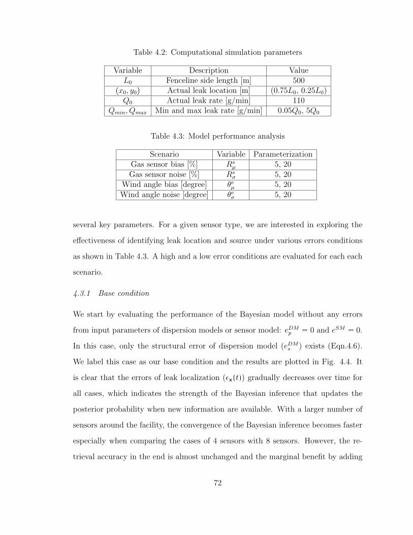
Table 4.2: Computational simulation parameters
Variable Description ValueL0 Fenceline side length [m] 500
px0, y0q Actual leak location [m] (0.75L0, 0.25L0)Q0 Actual leak rate [g/min] 110
Qmin, Qmax Min and max leak rate [g/min] 0.05Q0, 5Q0
Table 4.3: Model performance analysis
Scenario Variable ParameterizationGas sensor bias [%] Rs
µ 5, 20
Gas sensor noise [%] Rsσ 5, 20
Wind angle bias [degree] θeµ 5, 20
Wind angle noise [degree] θeσ 5, 20
several key parameters. For a given sensor type, we are interested in exploring the
effectiveness of identifying leak location and source under various errors conditions
as shown in Table 4.3. A high and a low error conditions are evaluated for each each
scenario.
4.3.1 Base condition
We start by evaluating the performance of the Bayesian model without any errors
from input parameters of dispersion models or sensor model: eDMp � 0 and eSM � 0.
In this case, only the structural error of dispersion model (eDMs ) exists (Eqn.4.6).
We label this case as our base condition and the results are plotted in Fig. 4.4. It
is clear that the errors of leak localization (εxptq) gradually decreases over time for
all cases, which indicates the strength of the Bayesian inference that updates the
posterior probability when new information are available. With a larger number of
sensors around the facility, the convergence of the Bayesian inference becomes faster
especially when comparing the cases of 4 sensors with 8 sensors. However, the re-
trieval accuracy in the end is almost unchanged and the marginal benefit by adding
72
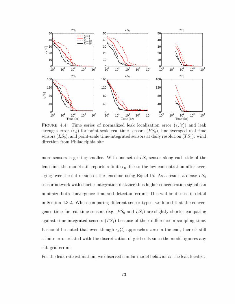
100
101
102
103
104
0
10
20
30
40
50
ǫX[%
]
PS0
K=4K=8K=12K=16
100
101
102
103
104
0
10
20
30
40
50LS0
100
101
102
103
104
0
10
20
30
40
50TS1
100
101
102
103
104
0
40
80
120
160
Time (hr)
ǫQ[%
]
PS0
100
101
102
103
104
0
40
80
120
160
Time (hr)
LS0
100
101
102
103
104
0
40
80
120
160
Time (hr)
TS1
Figure 4.4: Time series of normalized leak localization error (εxptq) and leakstrength error (εQ) for point-scale real-time sensors (PS0), line-averaged real-timesensors (LS0), and point-scale time-integrated sensors at daily resolution (TS1): winddirection from Philadelphia site
more sensors is getting smaller. With one set of LS0 sensor along each side of the
fenceline, the model still reports a finite εx due to the low concentration after aver-
aging over the entire side of the fenceline using Eqn.4.15. As a result, a dense LS0
sensor network with shorter integration distance thus higher concentration signal can
minimize both convergence time and detection errors. This will be discuss in detail
in Section 4.3.2. When comparing different sensor types, we found that the conver-
gence time for real-time sensors (e.g. PS0 and LS0) are slightly shorter comparing
against time-integrated sensors (TS1) because of their difference in sampling time.
It should be noted that even though εxptq approaches zero in the end, there is still
a finite error related with the discretization of grid cells since the model ignores any
sub-grid errors.
For the leak rate estimation, we observed similar model behavior as the leak localiza-
73
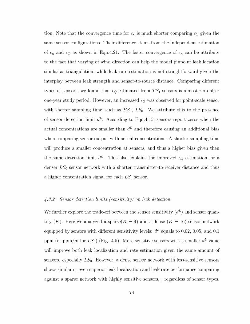
tion. Note that the convergence time for εx is much shorter comparing εQ given the
same sensor configurations. Their difference stems from the independent estimation
of εx and εQ as shown in Eqn.4.21. The faster convergence of εx can be attribute
to the fact that varying of wind direction can help the model pinpoint leak location
similar as triangulation, while leak rate estimation is not straightforward given the
interplay between leak strength and sensor-to-source distance. Comparing different
types of sensors, we found that εQ estimated from TS1 sensors is almost zero after
one-year study period. However, an increased εQ was observed for point-scale sensor
with shorter sampling time, such as PS0, LS0. We attribute this to the presence
of sensor detection limit dL. According to Eqn.4.15, sensors report zeros when the
actual concentrations are smaller than dL and therefore causing an additional bias
when comparing sensor output with actual concentrations. A shorter sampling time
will produce a smaller concentration at sensors, and thus a higher bias given then
the same detection limit dL. This also explains the improved εQ estimation for a
denser LS0 sensor network with a shorter transmitter-to-receiver distance and thus
a higher concentration signal for each LS0 sensor.
4.3.2 Sensor detection limits (sensitivity) on leak detection
We further explore the trade-off between the sensor sensitivity (dL) and sensor quan-
tity (K). Here we analyzed a sparse(K � 4) and a dense (K � 16) sensor network
equipped by sensors with different sensitivity levels: dL equals to 0.02, 0.05, and 0.1
ppm (or ppm/m for LS0) (Fig. 4.5). More sensitive sensors with a smaller dL value
will improve both leak localization and rate estimation given the same amount of
sensors. especially LS0. However, a dense sensor network with less-sensitive sensors
shows similar or even superior leak localization and leak rate performance comparing
against a sparse network with highly sensitive sensors, , regardless of sensor types.
74
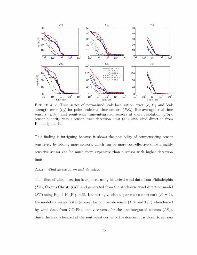
100
101
102
103
104
0
10
20
30
40
50
ǫX/L0[%
]
PS0
100
101
102
103
104
0
10
20
30
40
50LS0
100
101
102
103
104
0
10
20
30
40
50TS1
100
101
102
103
104
0
40
80
120
160
Time (hr)
ǫQ/Q
0[%
]
PS0
100
101
102
103
104
0
40
80
120
160
Time (hr)
LS0
dL = 0.1(K = 4)
dL = 0.05(K = 4)
dL = 0.02(K = 4)
dL = 0.1(K = 16)
dL = 0.05(K = 16)
dL = 0.02(K = 16)
100
101
102
103
104
0
40
80
120
160
Time (hr)
TS1
Figure 4.5: Time series of normalized leak localization error (εxptq) and leakstrength error (εQ) for point-scale real-time sensors (PS0), line-averaged real-timesensors (LS0), and point-scale time-integrated sensors at daily resolution (TS1):sensor quantity versus sensor lower detection limit (dL) with wind direction fromPhiladelphia site
This finding is intriguing because it shows the possibility of compensating sensor
sensitivity by adding more sensors, which can be more cost-effective since a highly
sensitive sensor can be much more expensive than a sensor with higher detection
limit.
4.3.3 Wind direction on leak detection
The effect of wind direction is explored using historical wind data from Philadelphia
(Ph), Corpus Christi (CC) and generated from the stochastic wind direction model
(ST ) using Eqn.4.10 (Fig. 4.6). Interestingly, with a sparse sensor network (K � 4),
the model converges faster (slower) for point-scale sensor (PS0 and TS1) when forced
by wind data from CC(Ph), and vice-versa for the line-integrated sensors (LS0).
Since the leak is located at the south-east corner of the domain, it is closer to sensors
75
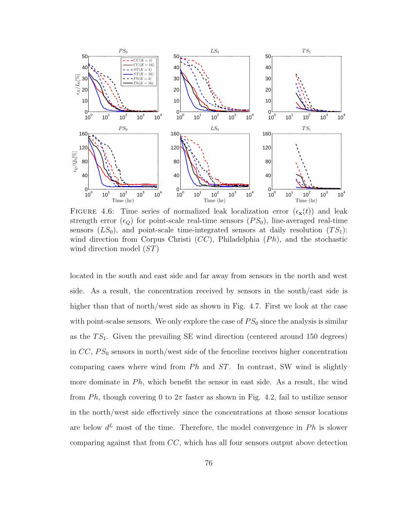
100
101
102
103
104
0
10
20
30
40
50
ǫX/L0[%
]
PS0
CC(K = 4)CC(K = 16)ST(K = 4)ST(K = 16)Ph(K = 4)Ph(K = 16)
100
101
102
103
104
0
10
20
30
40
50LS0
100
101
102
103
104
0
10
20
30
40
50TS1
100
101
102
103
104
0
40
80
120
160
Time (hr)
ǫQ/Q
0[%
]
PS0
100
101
102
103
104
0
40
80
120
160
Time (hr)
LS0
100
101
102
103
104
0
40
80
120
160
Time (hr)
TS1
Figure 4.6: Time series of normalized leak localization error (εxptq) and leakstrength error (εQ) for point-scale real-time sensors (PS0), line-averaged real-timesensors (LS0), and point-scale time-integrated sensors at daily resolution (TS1):wind direction from Corpus Christi (CC), Philadelphia (Ph), and the stochasticwind direction model (ST )
located in the south and east side and far away from sensors in the north and west
side. As a result, the concentration received by sensors in the south/east side is
higher than that of north/west side as shown in Fig. 4.7. First we look at the case
with point-scalse sensors. We only explore the case of PS0 since the analysis is similar
as the TS1. Given the prevailing SE wind direction (centered around 150 degrees)
in CC, PS0 sensors in north/west side of the fenceline receives higher concentration
comparing cases where wind from Ph and ST . In contrast, SW wind is slightly
more dominate in Ph, which benefit the sensor in east side. As a result, the wind
from Ph, though covering 0 to 2π faster as shown in Fig. 4.2, fail to ustilize sensor
in the north/west side effectively since the concentrations at those sensor locations
are below dL most of the time. Therefore, the model convergence in Ph is slower
comparing against that from CC, which has all four sensors output above detection
76
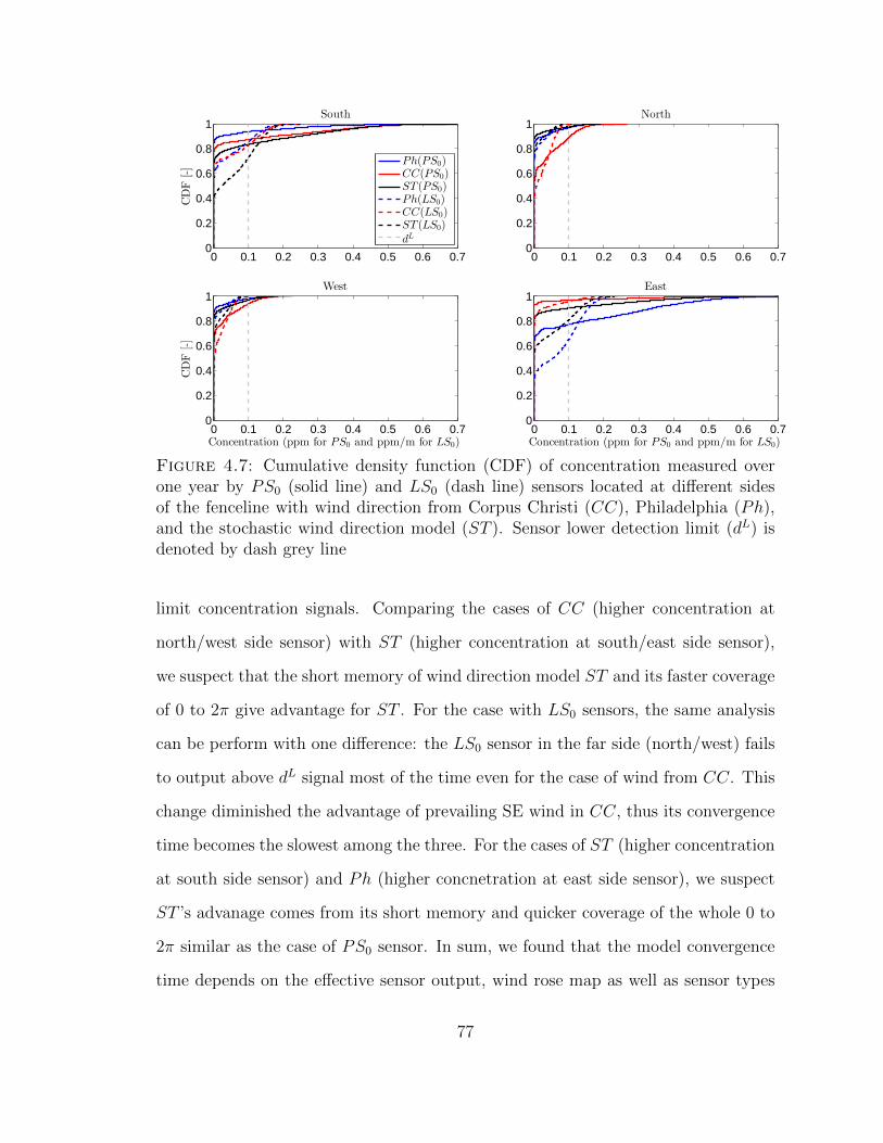
0 0.1 0.2 0.3 0.4 0.5 0.6 0.70
0.2
0.4
0.6
0.8
1South
CDF[-]
0 0.1 0.2 0.3 0.4 0.5 0.6 0.70
0.2
0.4
0.6
0.8
1North
0 0.1 0.2 0.3 0.4 0.5 0.6 0.70
0.2
0.4
0.6
0.8
1West
Concentration (ppm for PS0 and ppm/m for LS0)
CDF[-]
0 0.1 0.2 0.3 0.4 0.5 0.6 0.70
0.2
0.4
0.6
0.8
1East
Concentration (ppm for PS0 and ppm/m for LS0)
Ph(PS0)CC(PS0)ST (PS0)Ph(LS0)CC(LS0)ST (LS0)dL
Figure 4.7: Cumulative density function (CDF) of concentration measured overone year by PS0 (solid line) and LS0 (dash line) sensors located at different sidesof the fenceline with wind direction from Corpus Christi (CC), Philadelphia (Ph),and the stochastic wind direction model (ST ). Sensor lower detection limit (dL) isdenoted by dash grey line
limit concentration signals. Comparing the cases of CC (higher concentration at
north/west side sensor) with ST (higher concentration at south/east side sensor),
we suspect that the short memory of wind direction model ST and its faster coverage
of 0 to 2π give advantage for ST . For the case with LS0 sensors, the same analysis
can be perform with one difference: the LS0 sensor in the far side (north/west) fails
to output above dL signal most of the time even for the case of wind from CC. This
change diminished the advantage of prevailing SE wind in CC, thus its convergence
time becomes the slowest among the three. For the cases of ST (higher concentration
at south side sensor) and Ph (higher concnetration at east side sensor), we suspect
ST ’s advanage comes from its short memory and quicker coverage of the whole 0 to
2π similar as the case of PS0 sensor. In sum, we found that the model convergence
time depends on the effective sensor output, wind rose map as well as sensor types
77
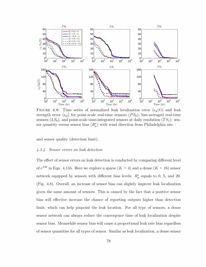
100
101
102
103
104
0
10
20
30
40
50
60
ǫX/L0[%
]
PS0
Rs
µ=0(K=4)
Rsµ=5(K=4)
Rsµ=20(K=4)
Rsµ=0(K=16)
Rsµ=5(K=16)
Rsµ=20(K=16)
100
101
102
103
104
0
10
20
30
40
50
60LS0
100
101
102
103
104
0
10
20
30
40
50
60TS1
100
101
102
103
104
0
40
80
120
160
Time (hr)
ǫQ/Q
0[%
]
PS0
100
101
102
103
104
0
40
80
120
160
Time (hr)
LS0
100
101
102
103
104
0
40
80
120
160
Time (hr)
TS1
Figure 4.8: Time series of normalized leak localization error (εxptq) and leakstrength error (εQ) for point-scale real-time sensors (PS0), line-averaged real-timesensors (LS0), and point-scale time-integrated sensors at daily resolution (TS1): sen-sor quantity versus sensor bias (Rs
µ) with wind direction from Philadelphia site
and sensor quality (detection limit).
4.3.4 Sensor errors on leak detection
The effect of sensor errors on leak detection is conducted by comparing different level
of eSM in Eqn. 4.15b. Here we explore a sparse (K � 4) and a dense (K � 16) sensor
network equipped by sensors with different bias levels: Rsµ equals to 0, 5, and 20.
(Fig. 4.8). Overall, an increase of sensor bias can slightly improve leak localization
given the same amount of sensors. This is caused by the fact that a positive sensor
bias will effective increase the chance of reporting outputs higher than detection
limit, which can help pinpoint the leak location. For all type of sensors, a dense
sensor network can always reduce the convergence time of leak localization despite
sensor bias. Meanwhile sensor bias will cause a proportional leak rate bias regardless
of sensor quantities for all types of sensor. Similar as leak localization, a dense sensor
78
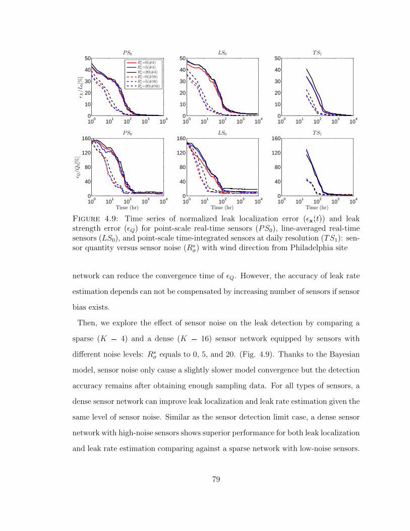
100
101
102
103
104
0
10
20
30
40
50
ǫX/L0[%
]
PS0
Rs
σ=0(#4)
Rsσ=5(#4)
Rsσ=20(#4)
Rsσ=0(#16)
Rsσ=5(#16)
Rsσ=20(#16)
100
101
102
103
104
0
10
20
30
40
50LS0
100
101
102
103
104
0
10
20
30
40
50TS1
100
101
102
103
104
0
40
80
120
160
Time (hr)
ǫQ/Q
0[%
]
PS0
100
101
102
103
104
0
40
80
120
160
Time (hr)
LS0
100
101
102
103
104
0
40
80
120
160
Time (hr)
TS1
Figure 4.9: Time series of normalized leak localization error (εxptq) and leakstrength error (εQ) for point-scale real-time sensors (PS0), line-averaged real-timesensors (LS0), and point-scale time-integrated sensors at daily resolution (TS1): sen-sor quantity versus sensor noise (Rs
σ) with wind direction from Philadelphia site
network can reduce the convergence time of εQ. However, the accuracy of leak rate
estimation depends can not be compensated by increasing number of sensors if sensor
bias exists.
Then, we explore the effect of sensor noise on the leak detection by comparing a
sparse (K � 4) and a dense (K � 16) sensor network equipped by sensors with
different noise levels: Rsσ equals to 0, 5, and 20. (Fig. 4.9). Thanks to the Bayesian
model, sensor noise only cause a slightly slower model convergence but the detection
accuracy remains after obtaining enough sampling data. For all types of sensors, a
dense sensor network can improve leak localization and leak rate estimation given the
same level of sensor noise. Similar as the sensor detection limit case, a dense sensor
network with high-noise sensors shows superior performance for both leak localization
and leak rate estimation comparing against a sparse network with low-noise sensors.
79
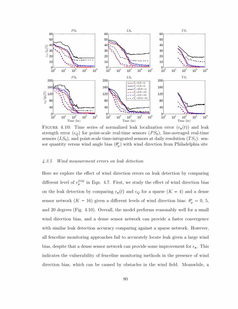
100
101
102
103
104
0
10
20
30
40
50
60
ǫ X/L0[%
]
PS0
100
101
102
103
104
0
10
20
30
40
50
60LS0
100
101
102
103
104
0
10
20
30
40
50
60TS1
100
101
102
103
104
0
40
80
120
160
200
Time (hr)
ǫ Q/Q
0[%
]
PS0
100
101
102
103
104
0
40
80
120
160
200
Time (hr)
LS0
θeµ=0(K=4)
θeµ=5(K=4)
θeµ=20(K=4)
θeµ=0(K=16)
θeµ=5(K=16)
θeµ=20(K=16)
100
101
102
103
104
0
40
80
120
160
200
Time (hr)
TS1
Figure 4.10: Time series of normalized leak localization error (εxptq) and leakstrength error (εQ) for point-scale real-time sensors (PS0), line-averaged real-timesensors (LS0), and point-scale time-integrated sensors at daily resolution (TS1): sen-sor quantity versus wind angle bias (θeµ) with wind direction from Philadelphia site
4.3.5 Wind measurement errors on leak detection
Here we explore the effect of wind direction errors on leak detection by comparing
different level of eDMp in Eqn. 4.7. First, we study the effect of wind direction bias
on the leak detection by comparing εxptq and εQ for a sparse (K � 4) and a dense
sensor network (K � 16) given a different levels of wind direction bias: θeµ = 0, 5,
and 20 degrees (Fig. 4.10). Overall, the model performs reasonably well for a small
wind direction bias, and a dense sensor network can provide a faster convergence
with similar leak detection accuracy comparing against a sparse network. However,
all fenceline monitoring approaches fail to accurately locate leak given a large wind
bias, despite that a dense sensor network can provide some improvement for εx. This
indicates the vulnerability of fenceline monitoring methods in the presence of wind
direction bias, which can be caused by obstacles in the wind field. Meanwhile, a
80
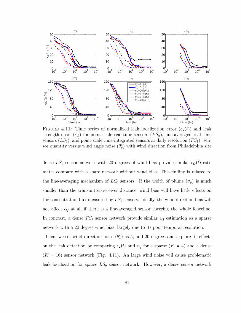
100
101
102
103
104
0
10
20
30
40
50
ǫX/L0[%
]
PS0
100
101
102
103
104
0
10
20
30
40
50LS0
100
101
102
103
104
0
10
20
30
40
50TS1
100
101
102
103
104
0
40
80
120
160
Time (hr)
ǫQ/Q
0[%
]
PS0
100
101
102
103
104
0
40
80
120
160
Time (hr)
LS0
θeσ=0(#4)θeσ=5(#4)θeσ=20(#4)θeσ=0(#16)θeσ=5(#16)θeσ=20(#16)
100
101
102
103
104
0
40
80
120
160
Time (hr)
TS1
Figure 4.11: Time series of normalized leak localization error (εxptq) and leakstrength error (εQ) for point-scale real-time sensors (PS0), line-averaged real-timesensors (LS0), and point-scale time-integrated sensors at daily resolution (TS1): sen-sor quantity versus wind angle noise (θeσ) with wind direction from Philadelphia site
dense LS0 sensor network with 20 degrees of wind bias provide similar εQptq esti-
mates compare with a spare network without wind bias. This finding is related to
the line-averaging mechanism of LS0 sensors. If the width of plume (σy) is much
smaller than the transmitter-receiver distance, wind bias will have little effects on
the concentration flux measured by LS0 sensors. Ideally, the wind direction bias will
not affect εQ at all if there is a line-averaged sensor covering the whole fenceline.
In contrast, a dense TS1 sensor network provide similar εQ estimation as a sparse
network with a 20 degree wind bias, largely due to its poor temporal resolution.
Then, we set wind direction noise (θeσ) as 5, and 20 degrees and explore its effects
on the leak detection by comparing εxptq and εQ for a sparse (K � 4) and a dense
(K � 16) sensor network (Fig. 4.11). An large wind noise will cause problematic
leak localization for sparse LS0 sensor network. However, a dense sensor network
81
can successfully improve leak localization despite wind noises. Overall, wind noise
will cause longer convergence time but can be quickly recovered when more mea-
surements become available due to the Bayesian updating scheme. In the end, the
accuracy of leak localization and leak rate are not greatly affected by wind noise
except for the sparse LS0 sensor network.
4.4 Conclusion
In this paper we propose a Bayesian inference model to evaluate leak detection skills
of different fenceline monitoring methods, including point scale sensors at real-time
(PS0), daily resolution (TS0), and line averaged sensors at real-time (LS0). First, we
tested the leak detection with only error from dispersion model, and we observed an
improved detection accuracy and faster convergence of estimates with a dense sensor
network. Then, we tested the effect of sensor sensitivity by comparing simulation
results with different levels of detection limits. The results is encouraging since we
found a trade-off between number of sensors and sensor detection limits, indicat-
ing that a dense sensor network has the potential of compensate low-sensitivity of
individual sensors. We further studied the effect of wind forcing data on Finally,
we performed some sensitivity test with varying levels of sensor and meteorological
errors. In sum, we found that all methods can partly correct noises from sensor or
wind direction when more measurements become available thanks to the Bayesian
scheme. Even though a higher sensor/wind direction noise will cause a slower model
convergence, it can be improved by adding more sensor nodes along the fenceline.
In contrast, all fenceline monitoring approaches fail to make an accurate leak rate
estimation when a sensor bias exists. However, they are still capable of pinpoint the
leak location, and a dense sensor network can produce a faster convergence. Mean-
while, time-integrated point-scale sensors can neither localize leak nor estimate its
leak strength. Though a dense LS0 or PS0 sensor network is able to reduce leak rate
82
given wind direction bias, they both fails to accurately localize the leak.
As we expected, a dense sensor network can always provide similar or faster conver-
gence for leak detection given the same level of sensor quality. This is encouraging
for applying low-cost sensor network with appropriate sensor detection limit for leak
localization. Comparing different methods, we find that real-time sensors such as
PS0 are slightly faster in leak localization and leak rate estimation, giving them
considerable advantage for application such as emission alarm systems. While time-
integrated sensors such as TS1 are more accurate when evaluated at the end of one
year study period, which is better for identifying annual leak budget from facilities.
LS0 sensors have distinctive advantage with the presence of wind direction bias,
which can be helpful given the distorted wind measurement due to facility obstacles
. However, its performance is also limited by sensor sensitivity. Overall, each type
of fenceline monitoring has its own strength and weakness and largely depends on
local conditions.
The model is heavily limited by our no-obstacle assumption. In reality, we would
anticipate errors in wind measurements along the path from the leak to the sensors.
The dispersion model used here is also a simple, and a CFD type of simulation tool
will be needed to better characterize wind field in the refinery. Also, our considera-
tion of single-source and continuous leaking is also a big simplification. In addition,
we did not consider sources from outside of the domain, such as nearby road and
pipelines.
83
5
A Mobile Sensing Approach for OperationalDetection of Fugitive Methane Emissions
5.1 Introduction
Given the detected amount of shale gas in continental U.S.[U.S. Energy Informa-
tion Adminstration (EIA) (2011)], natural gas is considered as a bridge fuel towards
clean energy due to its potential lower greenhouse gas (GHG) emission comparing
with other fossil fuels [Alvarez et al. (2012)]. Meanwhile, natural gas is the largest
source of anthropogenic emission of methane (CH4), which is a more potent GHG
than CO2. Natural gas leak could happen anywhere from its production to the end
users, thus jeopardizing its potential GHG reduction over competing fossil fuels such
as coal. There has been significant debates surrounding the aggregate magnitude of
fugitive emissions of natural gas. Much of the debate centers on whether the total
leak is above or below the tipping point of 3.2%, beyond which natural gas is consid-
ered to be worse than coal from a GHG reduction perspective [Alvarez et al. (2012)].
Current literature focuses on characterizing budgets of fugitive methane emissions
to improve the inventory of GHG emissions. Generally, sampling methods can be
84
categorized into top-down approaches, which estimate regional methane fluxes using
aerial platforms [Gentner et al. (2014); Caulton et al. (2014)], and bottom-up ap-
proaches, which conduct numerous in situ measurements of individual sites [Allen
et al. (2013)] to obtain a representative emission estimates of a certain type of indus-
try. Phillips et al. (2013) showed roadside methane concentrations in metropolitan
area of Boston, MA. using a mobile sensor. However, these efforts do not address the
practical need of identifying the location and strength of individual leaks in order to
guide direct mitigation efforts.
This work examines the feasibility of quantifying fugitive methane emission in sub-
urban and rural environments using a mobile sensor platform. A recently developed
plume integration method [Albertson et al. (2015)] is used to probabilistically infer
leak rate based on Bayesian inference and recursively update the estimates when
more information become available. Data collected from a series of controlled release
experiments is used to validate the mobile sensing method and compare against an-
other method [Brantley et al. (2014); U.S. Environmental Protection Agency (EPA)
(2014)]. Then, this mobile sensing approach is applied to estimate fugitive methane
emissions from several ammonia fertilizer plants based on field data. With access via
public roads, the mobile monitoring method is able to quickly assess the emission
strength of facilities. This work aims to develop the capacity of efficient regional
coverage of potential methane emissions in support of leak detection and mitigation
efforts.
5.2 Source inference from a mobile sensor
Foster-Wittig et al. (2015) developed a modified Gaussian plume model to identify
strength of fugitive methane emissions from a point source. Time series of methane
and meteorological data (around 20 minutes) collected by a sensor located in the
near- to middle- fields (18-200 meters downwind) was used as model input. Methane
85
concentration were binned according to wind direction to represent the ensemble
average. Instead of using stationary sensor data, Albertson et al. (2015) used data
collected by a mobile sensor platform and modified this approach by integrating
methane concentration across the plume. Comparing with the stationary approach,
this cross-plume integration method avoids the need to establish an ensemble av-
erage of plume concentration by oversampling in a mobile manner. However, the
performance of the mobile sensing approach has yet to be validated and compared
against the stationary method.
Here we briefly introduce the mobile sensing approach. Readers may refer to Albert-
son et al. (2015) for details. Consider a steady leak located at (x0) with a leak rate
of Q. Using a local coordinate system F � pX, Y, Zq with origin O at the leak source
and its X axis directed along the mean wind direction. The above-ambient ensem-
ble average plume concentration, Cpxq, can be modeled using a modified Gaussian
dispersion model [Pasquill and Smith (1983); Horst and Weil (1992)]:
Cpxq � QDypx, yqDzpx, zq
Upzq (5.1)
where Upzq is the effective speed of plume advection. Dypx, yq and Dzpx, zq are
the cross-wind and vertical dispersion factors, respectively [Horst and Weil (1992)].
The instantaneous and ensemble average are treated similarly given the cross-plume
sampling strategies [Albertson et al. (2015)]. Moreover, it is important to note that
we focus here on the scenario a single source. In practice, the measured concentration
can be a sum of multiple sources located upwind, which can be a straightforward
extension of the methods presented here.
In the cases of a mobile sensor traversing a plume along the path that is perpendicular
to the main wind direction, the cross-plume integral of Dy is unity (³8�8
Dypx, yqdy �1) when Dy is formulated in both instantaneous or ensemble-average manner. This
86
removes most of randomness caused by the lateral dispersion of instantaneous plumes.
The cross-plume integrated concentration can be represented as:
Cy �» 8
�8
Cpxqdy � QDzpx, zqUpzq (5.2)
where Cy is the cross-plume integrated concentration. Dz can be estimated as:
Dz � Az
exp
���Bzz
s�, where s, A, and B are functions of atmospheric stability
[Gryning et al. (1987); Foster-Wittig et al. (2015)]. Eqn.5.2 is strictly applicable only
when the path of the mobile sensor is perpendicular to the main wind direction.
In field applications, however, the sensor paths are typically limited by road access
that may not always perpendicular to the wind direction. In these cases, a numerical
integration of Eqn.5.2 can be used [Albertson et al. (2015)]:
Cy �8
i�0
Cpxiq∆tV � Q8
i�0
∆tV
Upziq�A
ziexp
���Bzzi
s�����
exp
�� 1
2
�yiσy
2�
?2πσy
��� (5.3)
where i is a index for the sensor position, ∆t is the sensor time step, V is the vehicle
speed, Dy is approximated by the traditional Gaussian shape function, σy is the
lateral dispersion length of the plume, and yi is the crosswind distance from the
plume center [Foster-Wittig et al. (2015); Albertson et al. (2015)].
Though individual mobile pass is not sufficient for source inference, we expect the
cumulative information gathered through multiple passes can be used to estimate leak
rate with each pass contributes partially to reduce the overall uncertainty. Therefore,
we treat the unknown leak rate as a random variable and apply a Bayesian inference
method that recursively updates the probability of leak rate after each pass with
reduced uncertainty. Comparing with the stationary method such as OTM33A [U.S.
Environmental Protection Agency (EPA) (2014)] and the Gaussian reconstruction
87
[Foster-Wittig et al. (2015)], this mobile sampling method simplified the need to
quantify plume lateral dispersion by integrating across-plume as shown in Eqn.5.2.
Also, the Bayesian inference method provide an updated estimate of the leak rate
in a quasi-real time manner, which provides an advantage for decision making in
real-world operational leak detection practice.
Following Bayes theorem, we can estimate the posterior probability density function
(pdf) of the source rate Q given the cross-plume integrated concentration Cy and
the local meteorological and landscape conditions I, such as surface roughness length
(z0) and atmospheric stability conditions.
ppQ|Cy, Iq � ppQqppCy|Q, IqppCy|Iq (5.4)
where ppQ|Cy, Iq, ppQq represent posterior and prior distribution of Q, respectively.
ppCy|Q, Iq is the likelihood function, which represents the probability of observing
Cy given Q. ppCy|Iq is the “evidence” which normalize the ppQ|Cy, Iq [Yee and
Flesch (2010)].
Prior to the sensing activities in a region of interest, we have no specific information
on the source rates of individual leaks. For a specific industrial facility, ppQq can be
roughly estimated given its structure and the leak potential/possibility of different
instruments. Also, past measurements can be served as a first estimate of ppQq as
shown in Brantley et al. (2014). For a general case, however, we adapt a uniform
distribution of Q assume that the upper (Qmax) and lower (Qmin) bounds of leak rate
are known. However, after jth successful samples of the leak, the recursive approach
update the prior as the ppQ|D, Iq of the previous pass.
ppQq �#
1{ pQmax �Qminq j � 1
ppQ|D, Iqj�1 j ¡ 1(5.5)
88
The likelihood function can be described by a traditional Gaussian likelihood function
[Yee and Flesch (2010)]:
ppD|Q, Iq � 1
σe?
2πexp
�� 1
2
�Cy � Cy
MpQqσe
2 �(5.6)
where CyMpQq is the integral of modeled cross-plume concentration for a given Q,
and σe is combined model and measurement errors Yee (2012). By integrating across
plume, this likelihood function becomes less sensitive to mismatches between actual
and modeled plume locations and widths, which is common due to plume meandering
and the randomness of turbulent dispersion.
Note that Eqn.5.6 assumes a unbiased estimate of Cy from CyMpQT q, where QT is
the actual leak rate. With known QT , we can estimate σe as:
σe �bEpCy � Cy
MpQT qq2 (5.7)
where the operator E denotes expectation estimation. Clearly Eqn. 5.7 is a function
of sensor error that will affect Cy and model error that will influence CyMpQT q. Be-
sides, atmospheric stability, landscape conditions such as the presence of obstacles
and surface roughness, and leak rate (QT ) itself all plays a role in the determination
of σe.
5.3 Source inference from a stationary sensor
Here we briefly introduce the OTM33A method [Brantley et al. (2014); U.S. En-
vironmental Protection Agency (EPA) (2014)]. The OTM33A method first bin the
concentration data according to the wind direction when the van is parked downwind
the source and estimate mean wind velocity U . Then, a Gaussian curve is used to
fit the binned wind direction against the concentration to obtained the peak concen-
tration (C). Finally, lateral (σy) and vertical (σz) dispersion are determined from a
89
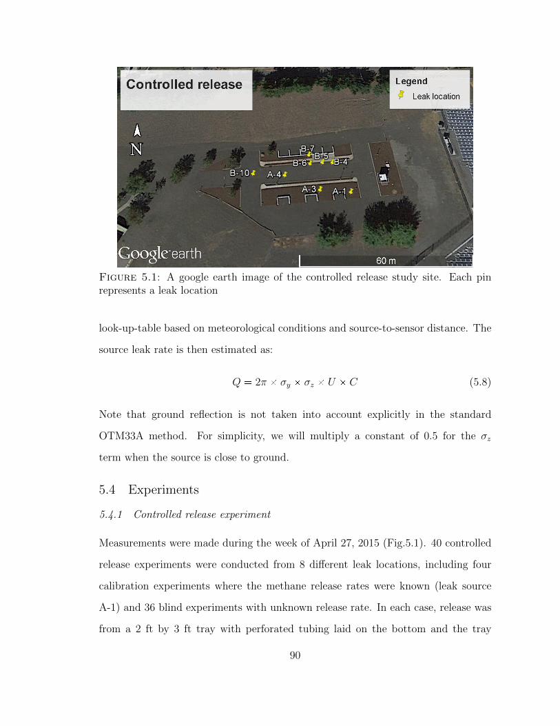
Figure 5.1: A google earth image of the controlled release study site. Each pinrepresents a leak location
look-up-table based on meteorological conditions and source-to-sensor distance. The
source leak rate is then estimated as:
Q � 2π � σy � σz � U � C (5.8)
Note that ground reflection is not taken into account explicitly in the standard
OTM33A method. For simplicity, we will multiply a constant of 0.5 for the σz
term when the source is close to ground.
5.4 Experiments
5.4.1 Controlled release experiment
Measurements were made during the week of April 27, 2015 (Fig.5.1). 40 controlled
release experiments were conducted from 8 different leak locations, including four
calibration experiments where the methane release rates were known (leak source
A-1) and 36 blind experiments with unknown release rate. In each case, release was
from a 2 ft by 3 ft tray with perforated tubing laid on the bottom and the tray
90
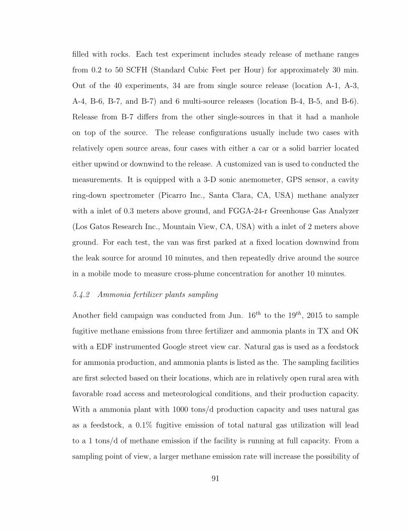
filled with rocks. Each test experiment includes steady release of methane ranges
from 0.2 to 50 SCFH (Standard Cubic Feet per Hour) for approximately 30 min.
Out of the 40 experiments, 34 are from single source release (location A-1, A-3,
A-4, B-6, B-7, and B-7) and 6 multi-source releases (location B-4, B-5, and B-6).
Release from B-7 differs from the other single-sources in that it had a manhole
on top of the source. The release configurations usually include two cases with
relatively open source areas, four cases with either a car or a solid barrier located
either upwind or downwind to the release. A customized van is used to conducted the
measurements. It is equipped with a 3-D sonic anemometer, GPS sensor, a cavity
ring-down spectrometer (Picarro Inc., Santa Clara, CA, USA) methane analyzer
with a inlet of 0.3 meters above ground, and FGGA-24-r Greenhouse Gas Analyzer
(Los Gatos Research Inc., Mountain View, CA, USA) with a inlet of 2 meters above
ground. For each test, the van was first parked at a fixed location downwind from
the leak source for around 10 minutes, and then repeatedly drive around the source
in a mobile mode to measure cross-plume concentration for another 10 minutes.
5.4.2 Ammonia fertilizer plants sampling
Another field campaign was conducted from Jun. 16th to the 19th, 2015 to sample
fugitive methane emissions from three fertilizer and ammonia plants in TX and OK
with a EDF instrumented Google street view car. Natural gas is used as a feedstock
for ammonia production, and ammonia plants is listed as the. The sampling facilities
are first selected based on their locations, which are in relatively open rural area with
favorable road access and meteorological conditions, and their production capacity.
With a ammonia plant with 1000 tons/d production capacity and uses natural gas
as a feedstock, a 0.1% fugitive emission of total natural gas utilization will lead
to a 1 tons/d of methane emission if the facility is running at full capacity. From a
sampling point of view, a larger methane emission rate will increase the possibility of
91
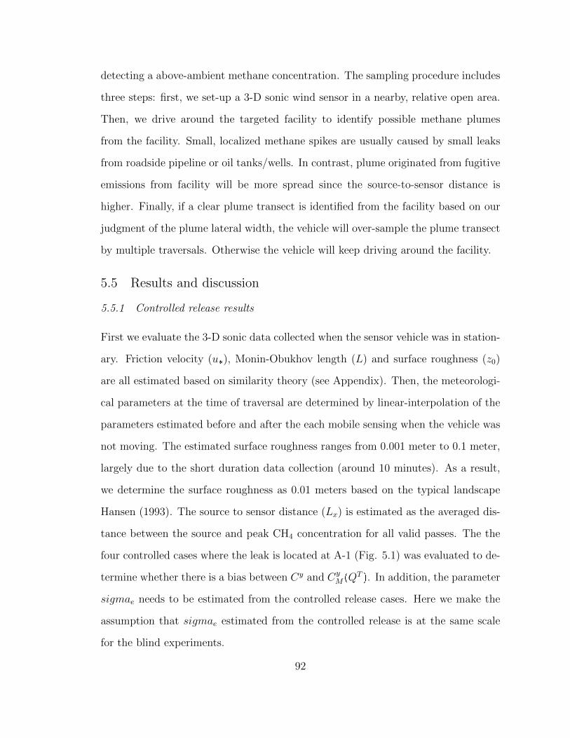
detecting a above-ambient methane concentration. The sampling procedure includes
three steps: first, we set-up a 3-D sonic wind sensor in a nearby, relative open area.
Then, we drive around the targeted facility to identify possible methane plumes
from the facility. Small, localized methane spikes are usually caused by small leaks
from roadside pipeline or oil tanks/wells. In contrast, plume originated from fugitive
emissions from facility will be more spread since the source-to-sensor distance is
higher. Finally, if a clear plume transect is identified from the facility based on our
judgment of the plume lateral width, the vehicle will over-sample the plume transect
by multiple traversals. Otherwise the vehicle will keep driving around the facility.
5.5 Results and discussion
5.5.1 Controlled release results
First we evaluate the 3-D sonic data collected when the sensor vehicle was in station-
ary. Friction velocity (u�), Monin-Obukhov length (L) and surface roughness (z0)
are all estimated based on similarity theory (see Appendix). Then, the meteorologi-
cal parameters at the time of traversal are determined by linear-interpolation of the
parameters estimated before and after the each mobile sensing when the vehicle was
not moving. The estimated surface roughness ranges from 0.001 meter to 0.1 meter,
largely due to the short duration data collection (around 10 minutes). As a result,
we determine the surface roughness as 0.01 meters based on the typical landscape
Hansen (1993). The source to sensor distance (Lx) is estimated as the averaged dis-
tance between the source and peak CH4 concentration for all valid passes. The the
four controlled cases where the leak is located at A-1 (Fig. 5.1) was evaluated to de-
termine whether there is a bias between Cy and CyMpQT q. In addition, the parameter
sigmae needs to be estimated from the controlled release cases. Here we make the
assumption that sigmae estimated from the controlled release is at the same scale
for the blind experiments.
92
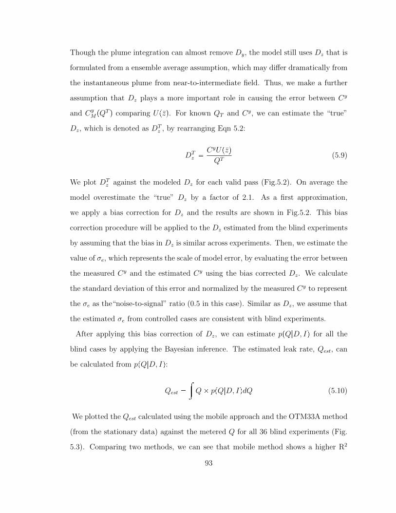
Though the plume integration can almost remove Dy, the model still uses Dz that is
formulated from a ensemble average assumption, which may differ dramatically from
the instantaneous plume from near-to-intermediate field. Thus, we make a further
assumption that Dz plays a more important role in causing the error between Cy
and CyMpQT q comparing Upzq. For known QT and Cy, we can estimate the “true”
Dz, which is denoted as DTz , by rearranging Eqn 5.2:
DTz �
CyUpzqQT
(5.9)
We plot DTz against the modeled Dz for each valid pass (Fig.5.2). On average the
model overestimate the “true” Dz by a factor of 2.1. As a first approximation,
we apply a bias correction for Dz and the results are shown in Fig.5.2. This bias
correction procedure will be applied to the Dz estimated from the blind experiments
by assuming that the bias in Dz is similar across experiments. Then, we estimate the
value of σe, which represents the scale of model error, by evaluating the error between
the measured Cy and the estimated Cy using the bias corrected Dz. We calculate
the standard deviation of this error and normalized by the measured Cy to represent
the σe as the“noise-to-signal” ratio (0.5 in this case). Similar as Dz, we assume that
the estimated σe from controlled cases are consistent with blind experiments.
After applying this bias correction of Dz, we can estimate ppQ|D, Iq for all the
blind cases by applying the Bayesian inference. The estimated leak rate, Qest, can
be calculated from ppQ|D, Iq:
Qest �»Q� ppQ|D, IqdQ (5.10)
We plotted the Qest calculated using the mobile approach and the OTM33A method
(from the stationary data) against the metered Q for all 36 blind experiments (Fig.
5.3). Comparing two methods, we can see that mobile method shows a higher R2
93
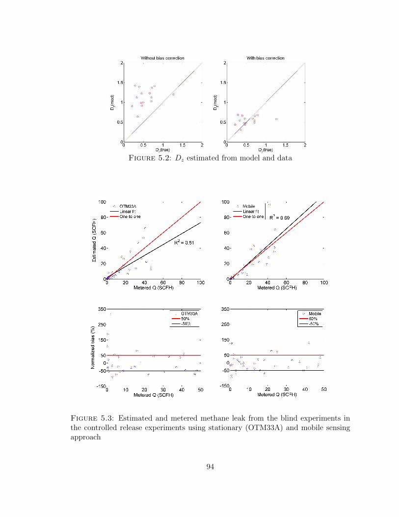
Figure 5.2: Dz estimated from model and data
Figure 5.3: Estimated and metered methane leak from the blind experiments inthe controlled release experiments using stationary (OTM33A) and mobile sensingapproach
94
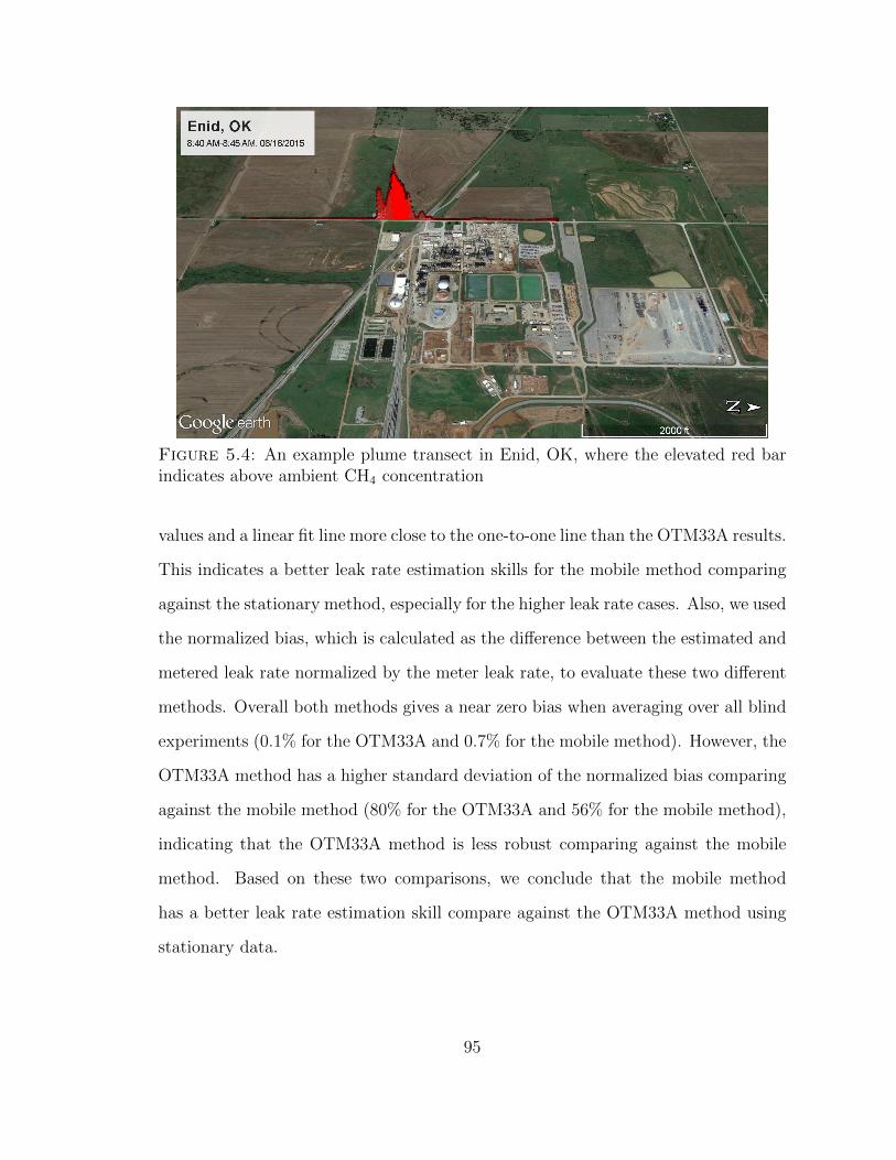
Figure 5.4: An example plume transect in Enid, OK, where the elevated red barindicates above ambient CH4 concentration
values and a linear fit line more close to the one-to-one line than the OTM33A results.
This indicates a better leak rate estimation skills for the mobile method comparing
against the stationary method, especially for the higher leak rate cases. Also, we used
the normalized bias, which is calculated as the difference between the estimated and
metered leak rate normalized by the meter leak rate, to evaluate these two different
methods. Overall both methods gives a near zero bias when averaging over all blind
experiments (0.1% for the OTM33A and 0.7% for the mobile method). However, the
OTM33A method has a higher standard deviation of the normalized bias comparing
against the mobile method (80% for the OTM33A and 56% for the mobile method),
indicating that the OTM33A method is less robust comparing against the mobile
method. Based on these two comparisons, we conclude that the mobile method
has a better leak rate estimation skill compare against the OTM33A method using
stationary data.
95
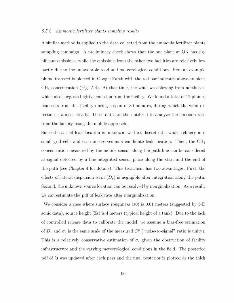
5.5.2 Ammonia fertilizer plants sampling results
A similar method is applied to the data collected from the ammonia fertilizer plants
sampling campaign. A preliminary check shows that the one plant at OK has sig-
nificant emissions, while the emissions from the other two facilities are relatively low
partly due to the unfavorable road and meteorological conditions. Here an example
plume transect is plotted in Google Earth with the red bar indicates above-ambient
CH4 concentration (Fig. 5.4). At that time, the wind was blowing from northeast,
which also suggests fugitive emission from the facility. We found a total of 12 plumes
transects from this facility during a span of 30 minutes, during which the wind di-
rection is almost steady. These data are then utilized to analyze the emission rate
from the facility using the mobile approach.
Since the actual leak location is unknown, we first discrete the whole refinery into
small grid cells and each one serves as a candidate leak location. Then, the CH4
concentration measured by the mobile sensor along the path line can be considered
as signal detected by a line-integrated sensor place along the start and the end of
the path (see Chapter 4 for details). This treatment has two advantages. First, the
effects of lateral dispersion term (Dy) is negligible after integration along the path.
Second, the unknown source location can be resolved by marginalization. As a result,
we can estimate the pdf of leak rate after marginalization.
We consider a case where surface roughness (z0) is 0.01 meters (suggested by 3-D
sonic data), source height (Zs) is 4 meters (typical height of a tank). Due to the lack
of controlled release data to calibrate the model, we assume a bias-free estimation
of Dz and σe is the same scale of the measured Cy (“noise-to-signal” ratio is unity).
This is a relatively conservative estimation of σe given the obstruction of facility
infrastructure and the varying meteorological conditions in the field. The posterior
pdf of Q was updated after each pass and the final posterior is plotted as the thick
96
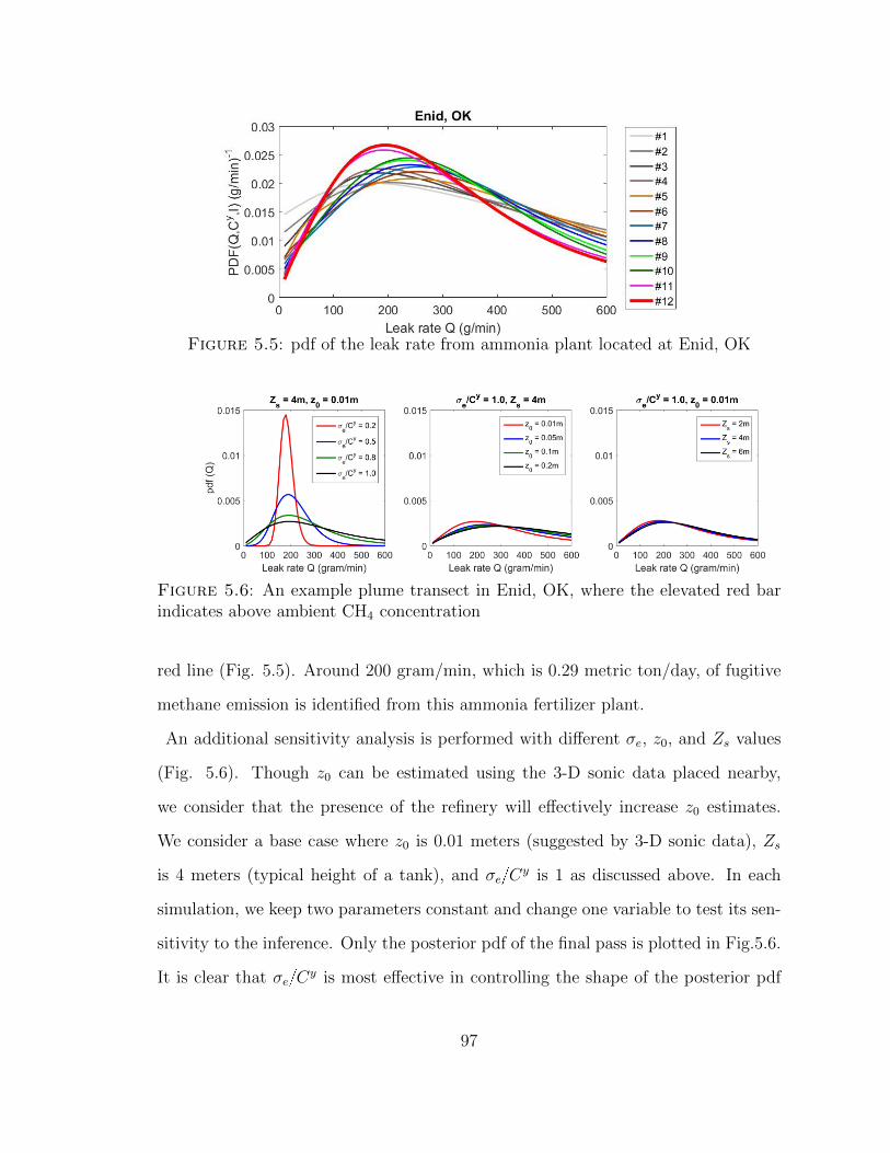
Figure 5.5: pdf of the leak rate from ammonia plant located at Enid, OK
Figure 5.6: An example plume transect in Enid, OK, where the elevated red barindicates above ambient CH4 concentration
red line (Fig. 5.5). Around 200 gram/min, which is 0.29 metric ton/day, of fugitive
methane emission is identified from this ammonia fertilizer plant.
An additional sensitivity analysis is performed with different σe, z0, and Zs values
(Fig. 5.6). Though z0 can be estimated using the 3-D sonic data placed nearby,
we consider that the presence of the refinery will effectively increase z0 estimates.
We consider a base case where z0 is 0.01 meters (suggested by 3-D sonic data), Zs
is 4 meters (typical height of a tank), and σe{Cy is 1 as discussed above. In each
simulation, we keep two parameters constant and change one variable to test its sen-
sitivity to the inference. Only the posterior pdf of the final pass is plotted in Fig.5.6.
It is clear that σe{Cy is most effective in controlling the shape of the posterior pdf
97
comparing with z0 and Zs. A small σe{Cy indicates higher confidence thus help the
inference converges faster with narrow pdf. Despite the different simulation results,
a leak rate around 200 gram/min, which is 0.29 metric ton/day of fugitive methane
emission is identified from this ammonia fertilizer plant.
5.6 Conclusion
Considerable success has been achieved using the mobile sensing approach for detect-
ing fugitive methane emission from suburban and rural environments. Comparing
with the OTM33A method using stationary data, the mobile methods can be more
effective in sampling emissions when the source is unknown and the wind is chang-
ing over time. In addition, it shows better skills in estimating leak rate comparing
against the OTM33A approach in the controlled release experiments.
The mobile method can be further improved in many different ways. Our first at-
tempt here is to remove its need of a prescribed leak location. However, we still
assume a single source scenario, which can be eliminated by constraining the space
of candidate leak locations and superimposing plumes from all of them. However,
more experiments and analytical work are need to further quantify the key param-
eters in the model such as Dz and σe under varying meteorological and obstacle
conditions.
98
6
Conclusion
Studies presented in this dissertation are motivated by the need to monitor environ-
mental and industrial state variables and their dynamics through sensor data. The
main objective is to utilize environmental data for source inference in a more sys-
tematic and rigorous way. The inference tools are developed based on the underlying
physical/chemical process that cause the phenomena. Meanwhile, data is evaluated
rigorously according to its specific application such that the problem of data redun-
dancy is directly addressed and data errors are included in our model evaluation and
predictions. Key findings from each chapter are summarized below.
In chapter 2, several different remote sensing data sets and retrieval algorithms were
used to retrieve suspended sediment concentration (SSC) in shallow water environ-
ment. For the hyperspectral remote sensing data, information redundancy and cross-
correlation were evaluated by comparing simulations using different combinations of
remote sensing bands and the result showed that a two-band combination is neces-
sary and almost sufficient to constrain the physically-based model. We also found
that the RMSE estimated using the leave-one-out cross-validation approach is a more
robust evaluation criterion comparing against the model calibration. When compar-
99
ing different retrieval methods, we found that the physically-based model has smaller
RMSE than two widely-used empirical models (linear and a 2nd order polynomial re-
gressions) using the same remote sensing data set. Meanwhile, the physically-based
model showed a wider applicability and robust performance with respect to band
selections of remote sensing data. This attribute can be beneficial when the ideal
bands suffer from low signal-to-noise ratio due to sensor malfunctioning or unfavor-
able atmospheric conditions, less preferable band combinations can be used without
introducing a significant amount of error. When comparing different remote sensing
data sets, our analysis implied that multispectral data with larger data archive can
provide more accurate retrieval of SSC in shallow waters comparing with hyperspec-
tral data. For SSC retrieval, the improved spectral resolution of the hyperspectral
data could not compensate for the lack of dataset partly due to its information re-
dundancy and cross-correlation. Though the Venice lagoon, Italy, is one of the most
densely monitored lagoon system in the world, we still face the challenge of obtain-
ing enough hyperspectral remote sensing data to validate our model. As a result,
we anticipate that the remote sensing retrieval of SSC using hyperspectral data to
be further deteriorated in other shallow water systems with sparse, short-term mon-
itoring stations.
In chapter 3, a novel sensor/sampling system (termed Kolibri) was developed for
mobile and aerial emission sampling of open area sources. Thanks to its compact
size, lightweight, and internal power supply, the Kolibri system can be carried by
unmanned aerial vehicles (UAVs) or aerostat system and is particularly suitable for
sampling missions with complex terrain and harsh environments. Onboard sensors
were selected based on laboratory testing for accuracy, delay and response, cross-
sensitivity, and precision. We first tested the Kolibri system against continuous
emission monitors (CEMs) and another sampling instrument (the “Flyer”). Our
results showed that the time series of CO2 and CO concentration and the PM2.5
100
measured by the Kolibri agreed well with those from the CEMs and the Flyer. The
emission factors of VOCs derived using the Kolibri are comparable with existing lit-
erature values. Then, we tested the effects of rotor wash on the PM2.5 distribution
using DustTrak and Kolibri systems in a indoor environment and the result showed
that the rotor wash has little effects on PM2.5 distribution under well-mixed condi-
tion. Finally, we utilized the Kolibri system for a open detonation sampling mission
and the measured PM2.5 emission factor are comparable with the value obtained
using the “Flyer” system.
In chapter 4, Bayesian inference method was introduced to detect and quantify fugi-
tive emission of gas and hazardous air pollutants using fenceline monitoring. The
strength and weakness of several existing fenceline monitoring methods are evalu-
ated under different kinds of sensor and model errors, which can be specified in the
Bayesian inference scheme. We found that all fenceline monitoring methods can
correct sensor noise thanks to the Bayesian method, however, they all fail to make
an accurate leak detection when a sensor/model bias exists. This finding suggested
that a bias-correction is necessary for the Bayesian inference, which can correct sen-
sor noise when more data become available. Under some circumstances, we found a
trade-off between sensor quality and quantity, indicating that a dense sensor network
has the potential of compensating the low-quality of individual sensors. This finding
suggests a cost-effective way to improve the performance of fenceline monitoring.
In chapter 5, a mobile sensing approach was introduced to estimate fugitive methane
emissions from industrial facilities and pipeline leaks in suburban and rural environ-
ments. We first tested the mobile sensing approach against a point source Gaussian
(PSG) approach [U.S. Environmental Protection Agency (EPA) (2014)] using a se-
ries of controlled release experiments. The mobile sensing model was first calibrated
by bias-correction of the vertical dispersion factors using a subset of measurements.
When evaluated using the rest dataset that are not included in the model calibration,
101
we found that the mobile sensing method can reduce estimation bias and uncertainty
comparing against the PSG approach. Then, we applied the mobile sensing approach
to quantify fugitive emissions from several ammonia fertilizer plants located in rural
areas. Significant methane emission was identified from one facility while the other
two shows relatively low emissions. Sensitivity analysis of several model parameters
showed that one parameter (error term in the Bayesian inference) was key to deter-
mine the model uncertainty while other two (surface roughness and source height)
were less influential. In sum, the mobile sensing approach showed considerable suc-
cess in quantifying fugitive methane emission, however, more field experiments are
needed to quantify the σe parameters in the future to help improve model perfor-
mance.
102
Appendix A
Modified Gaussian plume model (Chapter 4)
ψ is a dimensionless stability correction function, which can be estimated from Dyer
(1974)
ψpz{Lq �#p1 � 16z{Lq1{4 � 1 L 0
�5z{L L ¡ 0(A.1)
Upzq is the effective speed of plume advection at mean height z, which can be ap-
proximated following Gryning et al. (1987):
x1 � xc � z
κ2
#rlnp cz
z0q � p1 � a2
czLq1{4 � 1sr1 � pa1
z4Ls�1{2 L 0
rlnp czz0q � 2pb2
z3Lsr1 � pb1
z2Ls � pp b1
4� b2
6q zL
L ¡ 0(A.2)
where xc is a integration constant which accounts for the height of the source, zs. p
is an empirical constant (1.55). We used a1 � a2 � 16 and b1 � b2 � 5 following
Gryning Gryning et al. (1983). To solve for z, we first assign z � zs to solve for
x0. Then, z is estimated numerically through iteration with x1 set as the downwind
distance from the leak to the sensor and z � zm.
103
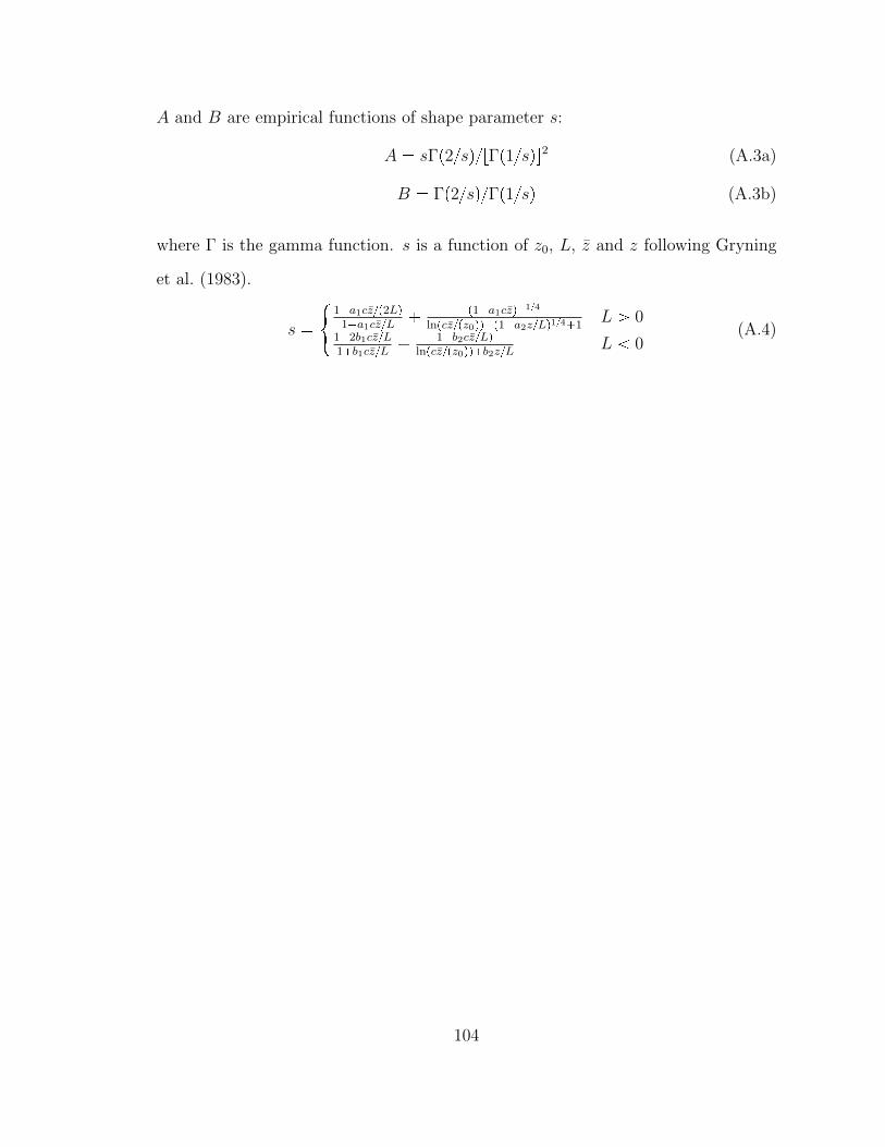
A and B are empirical functions of shape parameter s:
A � sΓp2{sq{rΓp1{sqs2 (A.3a)
B � Γp2{sq{Γp1{sq (A.3b)
where Γ is the gamma function. s is a function of z0, L, z and z following Gryning
et al. (1983).
s �#
1�a1cz{p2Lq1�a1cz{L
� p1�a1czq�1{4
lnpcz{pz0qq�p1�a2z{Lq1{4�1L ¡ 0
1�2b1cz{L1�b1cz{L
� 1�b2cz{Lqlnpcz{pz0qq�b2z{L
L 0(A.4)
104
Bibliography
Acharya, P. K., Berk, A., Bernstein, L. S., Matthew, M. W., Adler-Golden, S. M.,Robertson, D. C., Anderson, G. P., Chetwynd, J. H., Kneizys, F. X., and Shettle,E. P. (1998), “MODTRAN users manual versions 3.7 and 4.0,” Air Force ResearchLaboratory, Space Vehicles Directorate, Hanscom Air Force Base, Mass.
Albertson, J. D., Harvey, T., Foderaro, G., Zhu, P., Zhou, X., Ferrari, S., Amin,M. S., Modrak, M., Brantley, H., and Thoma, E. D. (2015), “A Mobile SensingApproach for Regional Surveillance of Fugitive Methane Emissions in Oil and GasProduction,” .
Allen, D. T., Torres, V. M., Thomas, J., Sullivan, D. W., Harrison, M., Hendler, A.,Herndon, S. C., Kolb, C. E., Fraser, M. P., Hill, A. D., Lamb, B. K., Miskimins,J., Sawyer, R. F., and Seinfeld, J. H. (2013), “Measurements of methane emissionsat natural gas production sites in the United States,” Proceedings of the NationalAcademy of Sciences, 110, 17768–17773.
Alvarez, R., Pacala, S., Winebrake, J., Chameides, W., and Hamburg, S. (2012),“Greater focus needed on methane leakage from natural gas infrastructure,” Pro-ceedings of the National Academy of Sciences, 109, 6435–6440.
Andreae, M. O. and Merlet, P. (2001), “Emission of trace gases and aerosols frombiomass burning,” Global biogeochemical cycles, 15, 955–966.
Aurell, J. and Gullett, B. K. (2013), “Emission factors from aerial and ground mea-surements of field and laboratory forest burns in the southeastern US: PM2. 5,black and brown carbon, VOC, and PCDD/PCDF,” Environmental science &technology, 47, 8443–8452.
Aurell, J., Gullett, B. K., Pressley, C., Tabor, D. G., and Gribble, R. D. (2011),“Aerostat-lofted instrument and sampling method for determination of emissionsfrom open area sources,” Chemosphere, 85, 806–811.
Aurell, J., Gullett, B. K., and Dennis, T. (2015), “Emissions from southeastern U.S.Grasslands and pine savannas: Comparison of aerial and ground field measure-ments with laboratory burns,” Atmospheric Environment, 111, 170–178.
105
Avissar, R., Holder, H. E., Abehserra, N., Bolch, M. A., Canning, P., Magalhaes, J.,Walko, R. L., Novick, K., Katul, G., Prince, K., et al. (2009), “The Duke Universityhelicopter observation platform,” Bulletin of the American Meteorological Society,90, 939–954.
Babin, M., Morel, A., Fournier-Sicre, V., Fell, F., and Stramski, D. (2003a), “Lightscattering properties of marine particles in coastal and open ocean waters as relatedto the particle mass concentration,” Limnology and Oceanography, 48, 843–859.
Babin, M., Stramski, D., Ferrari, G. M., Claustre, H., Bricaud, A., Obolensky, G.,and Hoepffner, N. (2003b), “Variations in the light absorption coefficients of phyto-plankton, nonalgal particles, and dissolved organic matter in coastal waters aroundEurope,” Journal of Geophysical Research-Oceans, 108.
Bajcsy, P. and Groves, P. (2004), “Methodology for hyperspectral band selection,”Photogrammetric Engineering and Remote Sensing, 70, 793–802.
Binding, C. E., Bowers, D. G., and Mitchelson-Jacob, E. G. (2005), “Estimatingsuspended sediment concentrations from ocean colour measurements in moder-ately turbid waters; the impact of variable particle scattering properties,” RemoteSensing of Environment, 94, 373–383.
Blum, M. D. and Roberts, H. H. (2009), “Drowning of the Mississippi Delta dueto insufficient sediment supply and global sea-level rise,” Nature Geoscience, 2,488–491.
Bond, T. C., Streets, D. G., Yarber, K. F., Nelson, S. M., Woo, J.-H., and Klimont,Z. (2004), “A technology-based global inventory of black and organic carbon emis-sions from combustion,” Journal of Geophysical Research: Atmospheres, 109.
Brando, V. E. and Dekker, A. G. (2003), “Satellite hyperspectral remote sensing forestimating estuarine and coastal water quality,” Ieee Transactions on Geoscienceand Remote Sensing, 41, 1378–1387.
Brantley, H., Thoma, E., Squier, W., Guven, B., and Lyon, D. (2014), “Assessmentof Methane Emissions from Oil and Gas Production using Mobile Measurements,”Environmental Science and Technology, 48, 14508–14515.
Brereton, C. A. and Johnson, M. R. (2012), “Identifying sources of fugitive emissionsin industrial facilities using trajectory statistical methods,” Atmospheric Environ-ment, 51, 46–55.
Burling, I., Yokelson, R. J., Akagi, S. K., Urbanski, S., Wold, C. E., Griffith, D.W. T., Johnson, T. J., Reardon, J., and Weise, D. (2011), “Airborne and ground-based measurements of the trace gases and particles emitted by prescribed fires inthe United States,” Atmospheric Chemistry and Physics, 11, 12197–12216.
106
Carniello, L., Defina, A., and D’Alpaos, L. (2009), “Morphological evolution of theVenice lagoon: Evidence from the past and trend for the future,” Journal of Geo-physical Research-Earth Surface, 114.
Carr, J., D’Odorico, P., McGlathery, K., and Wiberg, P. (2010), “Stability andbistability of seagrass ecosystems in shallow coastal lagoons: Role of feedbacks withsediment resuspension and light attenuation,” Journal of Geophysical Research-Biogeosciences, 115.
Caulton, D. R., Shepson, P. B., Santoro, R. L., Sparks, J. P., Howarth, R. W.,Ingraffea, A. R., Cambaliza, M. O., Sweeney, C., Karion, A., Davis, K. J., et al.(2014), “Toward a better understanding and quantification of methane emissionsfrom shale gas development,” Proceedings of the National Academy of Sciences,111, 6237–6242.
Chambers, A. K., Strosher, M., Wootton, T., Moncrieff, J., and McCready, P. (2008),“Direct measurement of fugitive emissions of hydrocarbons from a refinery,” Jour-nal of the Air & Waste Management Association, 58, 1047–1056.
Chen, Z. M., Hanson, J. D., and Curran, P. J. (1991), “The Form of the Relation-ship between Suspended Sediment Concentration and Spectral Reflectance - ItsImplications for the Use of Daedalus 1268 Data,” International Journal of RemoteSensing, 12, 215–222.
Christian, T. J., Kleiss, B., Yokelson, R. J., Holzinger, R., Crutzen, P., Hao, W. M.,Saharjo, B., and Ward, D. E. (2003), “Comprehensive laboratory measurementsof biomass-burning emissions: 1. Emissions from Indonesian, African, and otherfuels,” Journal of Geophysical Research: Atmospheres (1984–2012), 108.
Cofer, W., Winstead, E., Stocks, B., Goldammer, J., and Cahoon, D. (1998), “Crownfire emissions of CO2, CO, H2, CH4, and TNMHC from a dense jack pine borealforest fire,” Geophysical Research Letters, 25, 3919–3922.
Crutzen, P. J. and Andreae, M. O. (1990), “Biomass burning in the tropics: Impacton atmospheric chemistry and biogeochemical cycles,” Science, 250, 1669–1678.
D’Alpaos, A., Mudd, S. M., and Carniello, L. (2011), “Dynamic response of marshesto perturbations in suspended sediment concentrations and rates of relative sealevel rise,” Journal of Geophysical Research-Earth Surface, 116.
Datt, B., McVicar, T. R., Van Niel, T. G., Jupp, D. L. B., and Pearlman, J. S. (2003),“Preprocessing EO-1 Hyperion hyperspectral data to support the application ofagricultural indexes,” Ieee Transactions on Geoscience and Remote Sensing, 41,1246–1259.
107
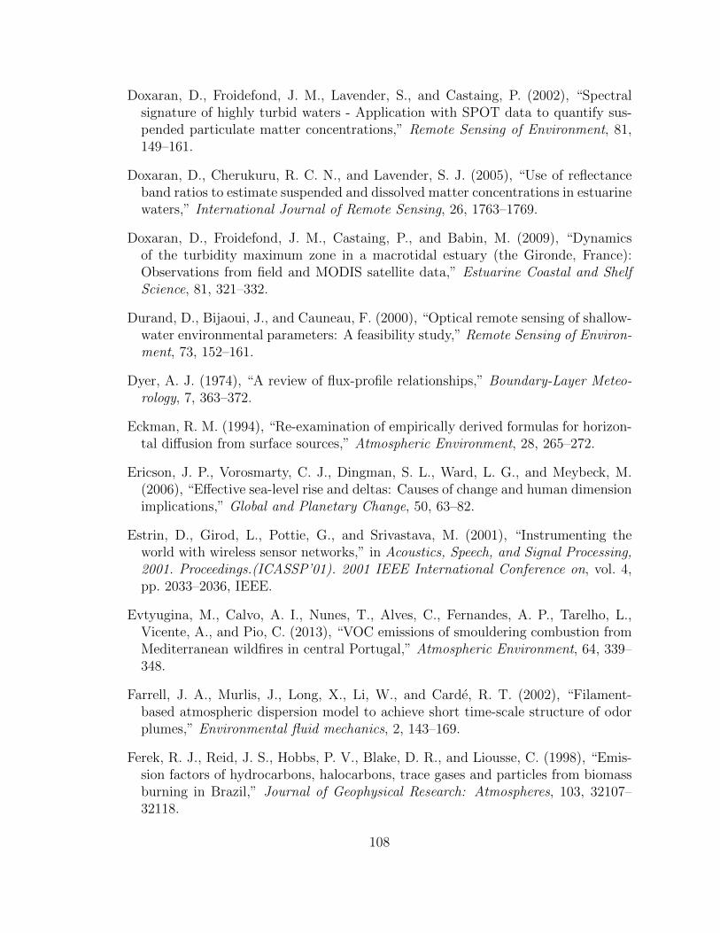
Doxaran, D., Froidefond, J. M., Lavender, S., and Castaing, P. (2002), “Spectralsignature of highly turbid waters - Application with SPOT data to quantify sus-pended particulate matter concentrations,” Remote Sensing of Environment, 81,149–161.
Doxaran, D., Cherukuru, R. C. N., and Lavender, S. J. (2005), “Use of reflectanceband ratios to estimate suspended and dissolved matter concentrations in estuarinewaters,” International Journal of Remote Sensing, 26, 1763–1769.
Doxaran, D., Froidefond, J. M., Castaing, P., and Babin, M. (2009), “Dynamicsof the turbidity maximum zone in a macrotidal estuary (the Gironde, France):Observations from field and MODIS satellite data,” Estuarine Coastal and ShelfScience, 81, 321–332.
Durand, D., Bijaoui, J., and Cauneau, F. (2000), “Optical remote sensing of shallow-water environmental parameters: A feasibility study,” Remote Sensing of Environ-ment, 73, 152–161.
Dyer, A. J. (1974), “A review of flux-profile relationships,” Boundary-Layer Meteo-rology, 7, 363–372.
Eckman, R. M. (1994), “Re-examination of empirically derived formulas for horizon-tal diffusion from surface sources,” Atmospheric Environment, 28, 265–272.
Ericson, J. P., Vorosmarty, C. J., Dingman, S. L., Ward, L. G., and Meybeck, M.(2006), “Effective sea-level rise and deltas: Causes of change and human dimensionimplications,” Global and Planetary Change, 50, 63–82.
Estrin, D., Girod, L., Pottie, G., and Srivastava, M. (2001), “Instrumenting theworld with wireless sensor networks,” in Acoustics, Speech, and Signal Processing,2001. Proceedings.(ICASSP’01). 2001 IEEE International Conference on, vol. 4,pp. 2033–2036, IEEE.
Evtyugina, M., Calvo, A. I., Nunes, T., Alves, C., Fernandes, A. P., Tarelho, L.,Vicente, A., and Pio, C. (2013), “VOC emissions of smouldering combustion fromMediterranean wildfires in central Portugal,” Atmospheric Environment, 64, 339–348.
Farrell, J. A., Murlis, J., Long, X., Li, W., and Carde, R. T. (2002), “Filament-based atmospheric dispersion model to achieve short time-scale structure of odorplumes,” Environmental fluid mechanics, 2, 143–169.
Ferek, R. J., Reid, J. S., Hobbs, P. V., Blake, D. R., and Liousse, C. (1998), “Emis-sion factors of hydrocarbons, halocarbons, trace gases and particles from biomassburning in Brazil,” Journal of Geophysical Research: Atmospheres, 103, 32107–32118.
108
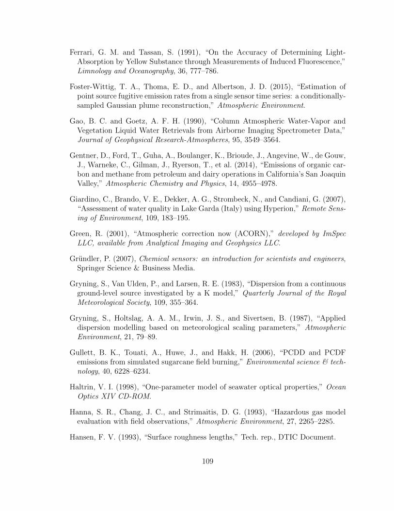
Ferrari, G. M. and Tassan, S. (1991), “On the Accuracy of Determining Light-Absorption by Yellow Substance through Measurements of Induced Fluorescence,”Limnology and Oceanography, 36, 777–786.
Foster-Wittig, T. A., Thoma, E. D., and Albertson, J. D. (2015), “Estimation ofpoint source fugitive emission rates from a single sensor time series: a conditionally-sampled Gaussian plume reconstruction,” Atmospheric Environment.
Gao, B. C. and Goetz, A. F. H. (1990), “Column Atmospheric Water-Vapor andVegetation Liquid Water Retrievals from Airborne Imaging Spectrometer Data,”Journal of Geophysical Research-Atmospheres, 95, 3549–3564.
Gentner, D., Ford, T., Guha, A., Boulanger, K., Brioude, J., Angevine, W., de Gouw,J., Warneke, C., Gilman, J., Ryerson, T., et al. (2014), “Emissions of organic car-bon and methane from petroleum and dairy operations in California’s San JoaquinValley,” Atmospheric Chemistry and Physics, 14, 4955–4978.
Giardino, C., Brando, V. E., Dekker, A. G., Strombeck, N., and Candiani, G. (2007),“Assessment of water quality in Lake Garda (Italy) using Hyperion,” Remote Sens-ing of Environment, 109, 183–195.
Green, R. (2001), “Atmospheric correction now (ACORN),” developed by ImSpecLLC, available from Analytical Imaging and Geophysics LLC.
Grundler, P. (2007), Chemical sensors: an introduction for scientists and engineers,Springer Science & Business Media.
Gryning, S., Van Ulden, P., and Larsen, R. E. (1983), “Dispersion from a continuousground-level source investigated by a K model,” Quarterly Journal of the RoyalMeteorological Society, 109, 355–364.
Gryning, S., Holtslag, A. A. M., Irwin, J. S., and Sivertsen, B. (1987), “Applieddispersion modelling based on meteorological scaling parameters,” AtmosphericEnvironment, 21, 79–89.
Gullett, B. K., Touati, A., Huwe, J., and Hakk, H. (2006), “PCDD and PCDFemissions from simulated sugarcane field burning,” Environmental science & tech-nology, 40, 6228–6234.
Haltrin, V. I. (1998), “One-parameter model of seawater optical properties,” OceanOptics XIV CD-ROM.
Hanna, S. R., Chang, J. C., and Strimaitis, D. G. (1993), “Hazardous gas modelevaluation with field observations,” Atmospheric Environment, 27, 2265–2285.
Hansen, F. V. (1993), “Surface roughness lengths,” Tech. rep., DTIC Document.
109
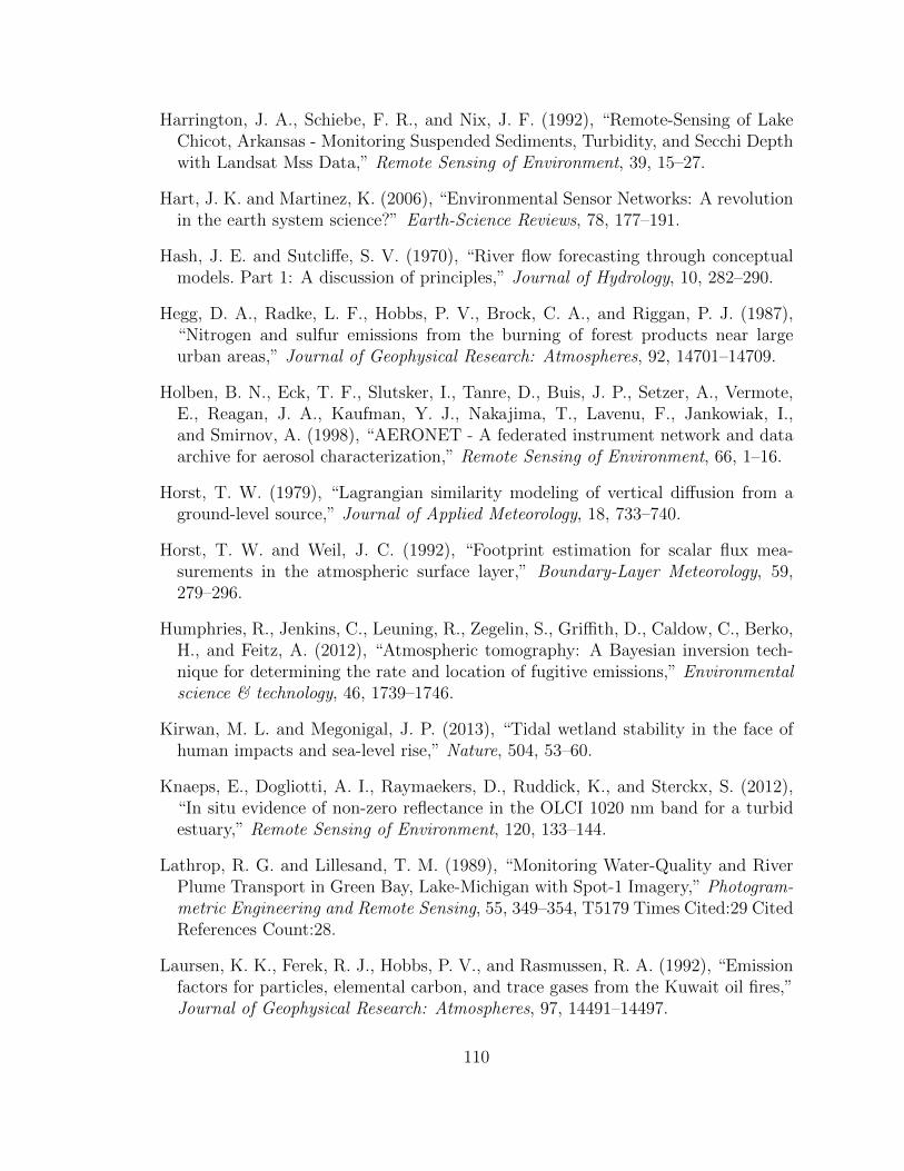
Harrington, J. A., Schiebe, F. R., and Nix, J. F. (1992), “Remote-Sensing of LakeChicot, Arkansas - Monitoring Suspended Sediments, Turbidity, and Secchi Depthwith Landsat Mss Data,” Remote Sensing of Environment, 39, 15–27.
Hart, J. K. and Martinez, K. (2006), “Environmental Sensor Networks: A revolutionin the earth system science?” Earth-Science Reviews, 78, 177–191.
Hash, J. E. and Sutcliffe, S. V. (1970), “River flow forecasting through conceptualmodels. Part 1: A discussion of principles,” Journal of Hydrology, 10, 282–290.
Hegg, D. A., Radke, L. F., Hobbs, P. V., Brock, C. A., and Riggan, P. J. (1987),“Nitrogen and sulfur emissions from the burning of forest products near largeurban areas,” Journal of Geophysical Research: Atmospheres, 92, 14701–14709.
Holben, B. N., Eck, T. F., Slutsker, I., Tanre, D., Buis, J. P., Setzer, A., Vermote,E., Reagan, J. A., Kaufman, Y. J., Nakajima, T., Lavenu, F., Jankowiak, I.,and Smirnov, A. (1998), “AERONET - A federated instrument network and dataarchive for aerosol characterization,” Remote Sensing of Environment, 66, 1–16.
Horst, T. W. (1979), “Lagrangian similarity modeling of vertical diffusion from aground-level source,” Journal of Applied Meteorology, 18, 733–740.
Horst, T. W. and Weil, J. C. (1992), “Footprint estimation for scalar flux mea-surements in the atmospheric surface layer,” Boundary-Layer Meteorology, 59,279–296.
Humphries, R., Jenkins, C., Leuning, R., Zegelin, S., Griffith, D., Caldow, C., Berko,H., and Feitz, A. (2012), “Atmospheric tomography: A Bayesian inversion tech-nique for determining the rate and location of fugitive emissions,” Environmentalscience & technology, 46, 1739–1746.
Kirwan, M. L. and Megonigal, J. P. (2013), “Tidal wetland stability in the face ofhuman impacts and sea-level rise,” Nature, 504, 53–60.
Knaeps, E., Dogliotti, A. I., Raymaekers, D., Ruddick, K., and Sterckx, S. (2012),“In situ evidence of non-zero reflectance in the OLCI 1020 nm band for a turbidestuary,” Remote Sensing of Environment, 120, 133–144.
Lathrop, R. G. and Lillesand, T. M. (1989), “Monitoring Water-Quality and RiverPlume Transport in Green Bay, Lake-Michigan with Spot-1 Imagery,” Photogram-metric Engineering and Remote Sensing, 55, 349–354, T5179 Times Cited:29 CitedReferences Count:28.
Laursen, K. K., Ferek, R. J., Hobbs, P. V., and Rasmussen, R. A. (1992), “Emissionfactors for particles, elemental carbon, and trace gases from the Kuwait oil fires,”Journal of Geophysical Research: Atmospheres, 97, 14491–14497.
110
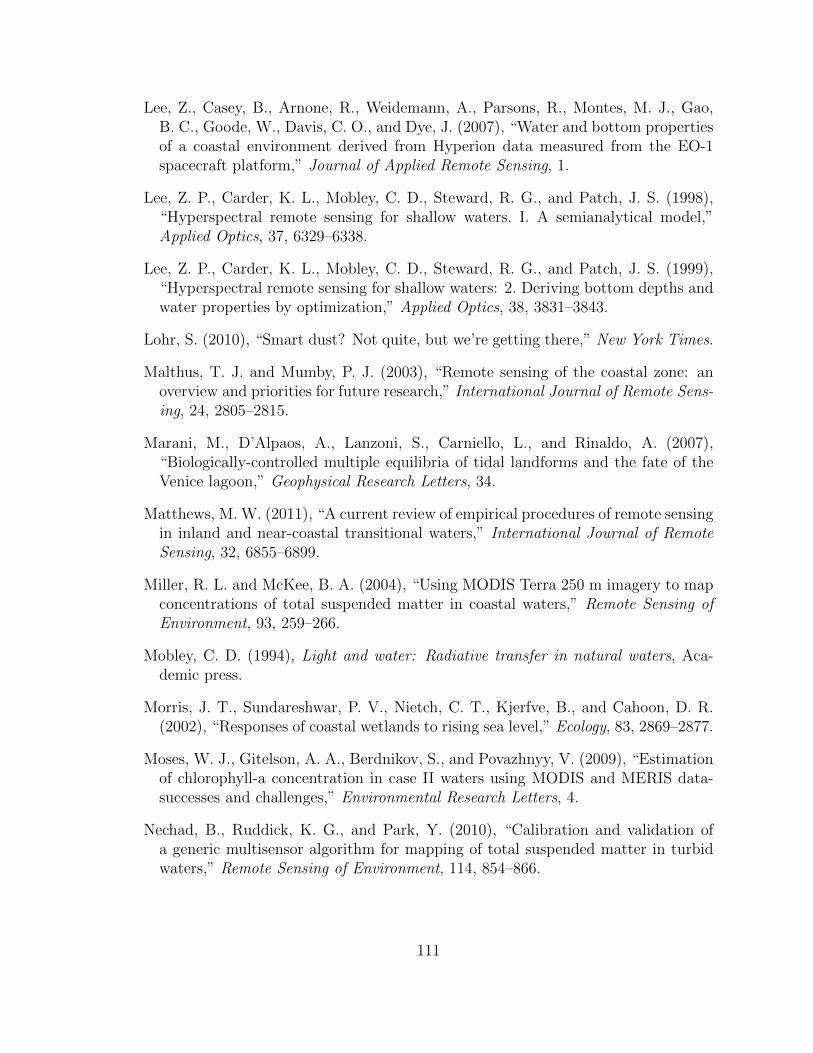
Lee, Z., Casey, B., Arnone, R., Weidemann, A., Parsons, R., Montes, M. J., Gao,B. C., Goode, W., Davis, C. O., and Dye, J. (2007), “Water and bottom propertiesof a coastal environment derived from Hyperion data measured from the EO-1spacecraft platform,” Journal of Applied Remote Sensing, 1.
Lee, Z. P., Carder, K. L., Mobley, C. D., Steward, R. G., and Patch, J. S. (1998),“Hyperspectral remote sensing for shallow waters. I. A semianalytical model,”Applied Optics, 37, 6329–6338.
Lee, Z. P., Carder, K. L., Mobley, C. D., Steward, R. G., and Patch, J. S. (1999),“Hyperspectral remote sensing for shallow waters: 2. Deriving bottom depths andwater properties by optimization,” Applied Optics, 38, 3831–3843.
Lohr, S. (2010), “Smart dust? Not quite, but we’re getting there,” New York Times.
Malthus, T. J. and Mumby, P. J. (2003), “Remote sensing of the coastal zone: anoverview and priorities for future research,” International Journal of Remote Sens-ing, 24, 2805–2815.
Marani, M., D’Alpaos, A., Lanzoni, S., Carniello, L., and Rinaldo, A. (2007),“Biologically-controlled multiple equilibria of tidal landforms and the fate of theVenice lagoon,” Geophysical Research Letters, 34.
Matthews, M. W. (2011), “A current review of empirical procedures of remote sensingin inland and near-coastal transitional waters,” International Journal of RemoteSensing, 32, 6855–6899.
Miller, R. L. and McKee, B. A. (2004), “Using MODIS Terra 250 m imagery to mapconcentrations of total suspended matter in coastal waters,” Remote Sensing ofEnvironment, 93, 259–266.
Mobley, C. D. (1994), Light and water: Radiative transfer in natural waters, Aca-demic press.
Morris, J. T., Sundareshwar, P. V., Nietch, C. T., Kjerfve, B., and Cahoon, D. R.(2002), “Responses of coastal wetlands to rising sea level,” Ecology, 83, 2869–2877.
Moses, W. J., Gitelson, A. A., Berdnikov, S., and Povazhnyy, V. (2009), “Estimationof chlorophyll-a concentration in case II waters using MODIS and MERIS data-successes and challenges,” Environmental Research Letters, 4.
Nechad, B., Ruddick, K. G., and Park, Y. (2010), “Calibration and validation ofa generic multisensor algorithm for mapping of total suspended matter in turbidwaters,” Remote Sensing of Environment, 114, 854–866.
111
Old, G. H., Leeks, G. J. L., Cooper, D., McNeil, D., and Smith, P. (2002), “Two tech-nological advances in continuous monitoring of suspended sediment transport andparticle characteristics,” Erosion and sediment transport measurement in rivers:Technological and methodological advances.
Pasquill, F. and Smith, F. B. (1983), Atmospheric diffusion: study of the dispersionof windborne material from industrial and other sources, JOHN WILEY & SONS,605 THIRD AVE., NEW YORK, NY 10016, USA.
Pearlman, J. S., Barry, P. S., Segal, C. C., Shepanski, J., Beiso, D., and Carman,S. L. (2003), “Hyperion, a space-based imaging spectrometer,” Ieee Transactionson Geoscience and Remote Sensing, 41, 1160–1173.
Petzold, T. J. (1972), “Volume scattering functions for selected ocean waters,” Re-port, DTIC Document.
Phillips, N. G., Ackley, R., Crosson, E. R., Down, A., Hutyra, L. R., Brondfield, M.,Karr, J. D., Zhao, K., and Jackson, R. B. (2013), “Mapping urban pipeline leaks:Methane leaks across Boston,” Environmental Pollution, 173, 1–4.
Piedrahita, R., Xiang, Y., Masson, N., Ortega, J., Collier, A., Jiang, Y., Li, K.,Dick, R., Lv, Q., Hannigan, M., et al. (2014), “The next generation of low-costpersonal air quality sensors for quantitative exposure monitoring,” AtmosphericMeasurement Techniques, 7, 3325–3336.
Pope, R. M. and Fry, E. S. (1997), “Absorption spectrum (380-700 nm) of purewater. II. Integrating cavity measurements,” Applied Optics, 36, 8710–8723.
Rao, K. S. (2005), “Uncertainty analysis in atmospheric dispersion modeling,” Pureand applied geophysics, 162, 1893–1917.
Ravera, O. (2000), “The Lagoon of Venice: the result of both natural factors andhuman influence,” Journal of Limnology, 59, 19–30.
Reid, J., Koppmann, R., Eck, T., and Eleuterio, D. (2005), “A review of biomassburning emissions part II: intensive physical properties of biomass burning parti-cles,” Atmospheric Chemistry and Physics, 5, 799–825.
Richter, R. and Schlpfer, D. (2007), “ATCOR-2/3 User Guide,” .
Ritchie, J. C., Zimba, P. V., and Everitt, J. H. (2003), “Remote sensing techniquesto assess water quality,” Photogrammetric Engineering and Remote Sensing, 69,695–704.
Santini, F., Alberotanza, L., Cavalli, R. M., and Pignatti, S. (2010), “A two-stepoptimization procedure for assessing water constituent concentrations by hyper-spectral remote sensing techniques: An application to the highly turbid Venicelagoon waters,” Remote Sensing of Environment, 114, 887–898.
112
Shi, W. and Wang, M. H. (2009), “An assessment of the black ocean pixel assumptionfor MODIS SWIR bands,” Remote Sensing of Environment, 113, 1587–1597.
Siebert, H., Lehmann, K., Wendisch, M., Franke, H., Maser, R., Schell, D., Wei Saw,E., and Shaw, R. A. (2006), “Probing finescale dynamics and microphysics ofclouds with helicopter-borne measurements,” Bulletin of the American Meteoro-logical Society, 87, 1727–1738.
Syvitski, J. P. M., Kettner, A. J., Overeem, I., Hutton, E. W. H., Hannon, M. T.,Brakenridge, G. R., Day, J., Vorosmarty, C., Saito, Y., Giosan, L., and Nicholls,R. J. (2009), “Sinking deltas due to human activities,” Nature Geoscience, 2, 681–686.
Thoma, E. D., Miller, M. C., Chung, K. C., Parsons, N. L., and Shine, B. C. (2011),“Facility Fence-Line Monitoring Using Passive Samplers,” Journal of the Air &Waste Management Association, 61, 834–842.
Thoma, E. D., Jiao, W., Brantley, H., Wu, T., Squier, W., Mitchell, W., Oliver,K., Whitaker, D., S, M., Colon, M., Alston, L., Gross-Davis, C. A., Schmidt,H., Landy, R., DeWees, J., R., M., Escobar, E., Amin, S. M., Modrak, M., andCousett, T. (2015), “South Philadelphia Passive Sampler and Sensor Study: In-terim Report,” .
Tyler, A. N., Svab, E., Preston, T., Presing, M., and Kovacs, W. A. (2006), “Remotesensing of the water quality of shallow lakes: A mixture modelling approach toquantifying phytoplankton in water characterized by high-suspended sediment,”International Journal of Remote Sensing, 27, 1521–1537.
U.S. Energy Information Adminstration (EIA) (2011), “Natural Gas Annual Re-port.” .
U.S. Environmental Protection Agency (EPA) (2014), “Other Test Method OTM33A Geospatial Measurement of Air Pollution-Remote Emissions Quantification-Direct Assessment (GMAP-REQ-DA),” .
U.S. Environmental Protection Agency (EPA) (2015a), “Inventory of US GreenhouseGas Emissions and Sinks: 1990-2013,” .
U.S. Environmental Protection Agency (EPA) (2015b), “Petroleum Refinery SectorRisk and Technology Review and New Source Performance Standards,” .
van Ulden, A. P. (1978), “Simple estimates for vertical diffusion from sources nearthe ground,” Atmospheric Environment, 12, 2125–2129.
Vermote, E. F. and Kotchenova, S. (2008), “Atmospheric correction for the monitor-ing of land surfaces,” Journal of Geophysical Research-Atmospheres, 113.
113
Volpe, V., Silvestri, S., and Marani, M. (2011), “Remote sensing retrieval of sus-pended sediment concentration in shallow waters,” Remote Sensing of Environ-ment, 115, 44–54.
Wang, F., Han, L., Kung, H. T., and van Arsdale, R. B. (2006), “Applications ofLandsat-5 TM imagery in assessing and mapping water quality in Reelfoot Lake,Tennessee,” International Journal of Remote Sensing, 27, 5269–5283.
Wang, H. J., Saito, Y., Zhang, Y., Bi, N. S., Sun, X. X., and Yang, Z. S. (2011),“Recent changes of sediment flux to the western Pacific Ocean from major riversin East and Southeast Asia,” Earth-Science Reviews, 108, 80–100.
Wang, X. J. and Ma, T. (2001), “Application of remote sensing techniques in moni-toring and assessing the water quality of Taihu Lake,” Bulletin of EnvironmentalContamination and Toxicology, 67, 863–870, 492CT Times Cited:12 Cited Refer-ences Count:11.
White, D. (2013), “Hyperion Tools 2.0 Installation and User Guide,” Report.
Wilks, D. S. (2006), Statistical methods in the atmospheric sciences, Internationalgeophysics series, Academic Press, Amsterdam ; Boston, 2nd edn.
WMO (2008), Guide to Meteorological Instruments and Methods of Observation(WMO-No.8), World Meteorological Organisation.
Yang, S. L., Milliman, J. D., Li, P., and Xu, K. (2011), “50,000 dams later: Erosionof the Yangtze River and its delta,” Global and Planetary Change, 75, 14–20.
Yee, E. (2007), “Bayesian probabilistic approach for inverse source determinationfrom limited and noisy chemical or biological sensor concentration measurements,”in Defense and Security Symposium, pp. 65540W–65540W, International Societyfor Optics and Photonics.
Yee, E. (2008), “Theory for reconstruction of an unknown number of contaminantsources using probabilistic inference,” Boundary-layer meteorology, 127, 359–394.
Yee, E. (2012), “Probability Theory as Logic: Data Assimilation for Multiple SourceReconstruction,” Pure and Applied Geophysics, 169, 499–517.
Yee, E. and Flesch, T. (2010), “Inference of emission rates from multiple sources usingBayesian probability theory,” Journal of Environmental Monitoring, 12, 622–634.
114
Biography
Xiaochi Zhou was born on March 29, 1987 in Changsha, Hunan, People’s Republic
of China. Xiaochi received his B.Eng. degree from School of Water Resources and
Hydropower, Wuhan University (China) in 2009 and a M.S.C.E degree from Depart-
ment of Civil and Environmental Engineering, University of Washington, Seattle in
2011. Based on his Ph.D. research at Duke, Xiaochi has coauthored 3 journal arti-
cles under review and 3 under preparation. He also served as a part-time student
service contractor at USEPA, office of research and development at RTP under the
supervision of Dr. Brian K. Gullett.
115