Novel Algorithms for Modeling Sedimentation and Compaction using 3D Unstructured Meshes.

Ulisses T. Mello - IBM T. J. Watson Research Center, Yorktown Heights, NY, 10598 José R. P. Rodrigues - PETROBRÁS R&D Center (CENPES), Rio de Janeiro, Brazil Paulo R. Cavalcanti - Federal University of Rio de Janeiro, Rio de Janeiro, Brazil

Abstract In this paper, we discuss some novel techniques for modeling sedimentation and compaction using fully unstructured meshes. The numerical modeling of the sedimentation process is a critical part of basin simulation and synthetic stratigraphy modeling. Normally, structured curvilinear meshes are used to represent sedimentary sequences to be deposited during the simulation. Using this approach, 2D grids represent layers of newly deposited sediments of a sequence during the simulation. In simulations that involve compaction, the 3D meshes are restricted to have vertical planes parallel to depth direction in order to accommodate the compaction calculation since most compaction algorithms in basin modeling are essentially one-dimensional. This kind of curvilinear mesh poses severe limitations to represent complex geological structures such as non-vertical faults, pinch-outs and salt domes. Unstructured meshes are much more flexible for representing complex geometry. We have developed new algorithms to use arbitrarily defined unstructured meshes for modeling numerically sedimentation and compaction in 2D and 3D. These algorithms (1) allow the generation of stratigraphic meshes by solving the Laplace equation to generate isosurfaces representing time lines that constrain the triangulation and (2) use a Streamline Upwind Finite Element formulation (SUPG) to calculate compaction during the simulation of evolving sedimentary basins. These algorithms have being applied with success in a 3D multiphase fluid flow simulator that we are developing to handle complex geometries with distinct degrees of mesh refinement/resolution during the simulation.

Introduction In many geoscientific applications, a flexible discretization method is extremely useful in the definition of complex geological geometries, discontinuity, and to enhance the resolution close to areas of interest. Traditional Cartesian grids with finite difference methods are not appropriate for representing complex geometries or grid refinement. It is desirable to adopt the intrinsic mesh flexibility of finite element or finite volume methods to simulate numerically geological processes. Although curvilinear grids are extensively used in the literature (e.g., Bathke, 1985; Burrus & Audebert, 1990), they do not provide

sufficient flexibility to align the grids with arbitrarily shaped geological structures such as salt domes, pinch-outs, faults and etc. Additional limitations arise to align structured grids with varying permeability and conductivity tensors, when solving heat and fluid transfer equations. Flexible unstructured meshes overcome limitations of the structured grids (Cartesian and curvilinear). Despite the advantages of unstructured meshes for representing complex geometries, their use is not widespread due to the lack of algorithms to take advantage of unstructured grids. In this paper, we suggest novel techniques for fully exploit the intrinsic flexibility of unstructured meshes to model sedimentation and compaction. These techniques are being applied with success in a 3D multi-phase and single-phase fluid flow simulator that we are developing to handle complex geometries with distinct degrees of mesh refinement and resolution during the simulation. In the following sections, we present a brief summary about the advantages and limitations of the most commonly adopted meshing strategies in basin modeling, then we present a technique to generate stratigraphic meshes in 2D and 3D for modeling sedimentation and compaction. In the sequel, we discuss a method to calculate the lithostatic pressure and compaction of sediments in 2D and 3D that does not required the mesh cells to be separated by vertical planes or lines. At the end, we apply these techniques to simple test cases to demonstrate their correctness and accuracy.

Meshing and basin representation In this section we discuss the advantages and limitations of the most common gridding strategies used to represent geological objects in basin modeling.

Curvilinear grids Curvilinear grids (Figure 1) are one the most popular form of discretization of geological layers for basin modeling and reservoir simulation. This kind of grid has various advantages: (1) it is relatively easy to generate in 2D and (2) there are many algorithms available for 2D cases (e.g., Knupp & Steinberg, 1993). Because these grids are structured, or regular, it is simple to obtain adjacency information from neighboring cells because they have constant and implicit adjacency. In addition, cells, or elements, of a structured curvilinear grid can be addressed programmatically by a triplet of indices, (i, j, k), which is quite convenient for finite difference methods. Irregular basin layers can be mapped with finite difference grid by making the x-direction curvilinear along stratigraphic time lines and maps it to the i-direction of the computational grid. This characteristic makes curvilinear grids highly adaptable to represent lateral heterogeneities, and to be used efficiently with geostatistical algorithms with one variogram for each major axis of the grid.

The disadvantages of curvilinear grids become apparent in Figure 1. If one wishes to represent the border of a basin accurately without truncation (Figure 2), the quadrangular elements close to the border would become degenerated since it would have to become triangular in shape. This problem is accentuated in cases of complex geometries such as salt domes. In addition, if internal boundaries representing faults and fractures are necessary in simulations, the generation of conformal curvilinear grids including internal boundaries is more complex (e.g., Shape & Anderson, 1990). In addition, these algorithms are not easily extendable to 3D, especially if grid orthogonality is required. It is important to note that the grid displayed in Figure 1b is clearly non-orthogonal. Non-orthogonal grids produce cross-flow terms in the solution of heat and fluid transfer problems, resulting in inaccurate solutions if the full cross-derivative terms are not included in the numerical solution (and they are normally not). Another significant limitation is the representation of anisotropy in these grids. If anisotropy does not align with the time lines in the grid, it extremely difficult, if not impossible, to generate a grid that aligns to arbitrary directions of anisotropy and stratigraphic time lines simultaneously.

Meshes based on triangle-strips This class of meshes emerged out of the need for more flexibility in representing geological features such as pinch-outs and borders of basins. Typical examples of this class of meshes can be found in Person & Garven (1989) and Bitzer (1996) in which geological layers are represented by a strip of triangles properly connected between two time lines (Figure 3). Although the generation of this kind of mesh is not much more difficult than the curvilinear grids, it provides much greater flexibility in terms of geometry representation and anisotropy discretization. Even simple cases of salt motion can be handled by this meshing technique (e.g., Mello et al., 1995). In theory, this class of meshes can be extended to 3D but usually they present the same sort of limitations in terms of geometry that curvilinear grids possess. This happens because they are generated in two steps. First the generation of a curvilinear grid that is then, in a second step, converted to a tetrahedral grid. This conversion is performed by subdividing each hexagonal element into 5 or 6 tetrahedral elements. However, in terms of anisotropy discretization, triangular and tetrahedral elements can accommodate arbitrary anisotropy directions easily if methods such as Finite Element and Finite Volumes are used (e.g., Zienkiewicz et al., 1966). Despite the greater flexibility of this class of meshes, they are not fully exploited for basin modeling applications due to the lack of algorithms that can handle compaction in 2D or 3D. In basin modeling, compaction is assumed to occur only in the vertical direction and it is considered essentially a one-dimensional process (e.g., Athy, 1930). To take advantage of 1D compaction algorithms (Sclater & Christie, 1980; Bethke, 1985), 2D and 3D meshes are restricted to have vertical planes parallel to depth direction (Figure 3b). Similarly to curvilinear grids, this severely restricts the ability of these meshes to represent complex geological structures.

Unstructured triangular and tetrahedral meshes Fully unstructured meshes are the most flexible to represent both complex geometry and anisotropy (Figure 4). The generation of triangular and tetrahedral meshes for arbitrary shapes is well understood (e.g., George, 2000) and Delaunay triangulations can be applied effectively to create meshes for very complex geological shapes (Cavalcanti & Mello, 1999; Mello & Cavalcanti, 2000). Unlike the triangle-strip based meshes, the generation of unstructured meshes is straightforward and they do not require an initial curvilinear grid. This is very advantageous for steady-state simulations in which sedimentation and active compaction is not modeled. However, in order to model sedimentation, unstructured meshes must be constrained by boundaries and by predefined stratigraphic time lines of the geological layer. This can be achieved using constrained Delaunay triangulation methods, as it will be described in the following section.

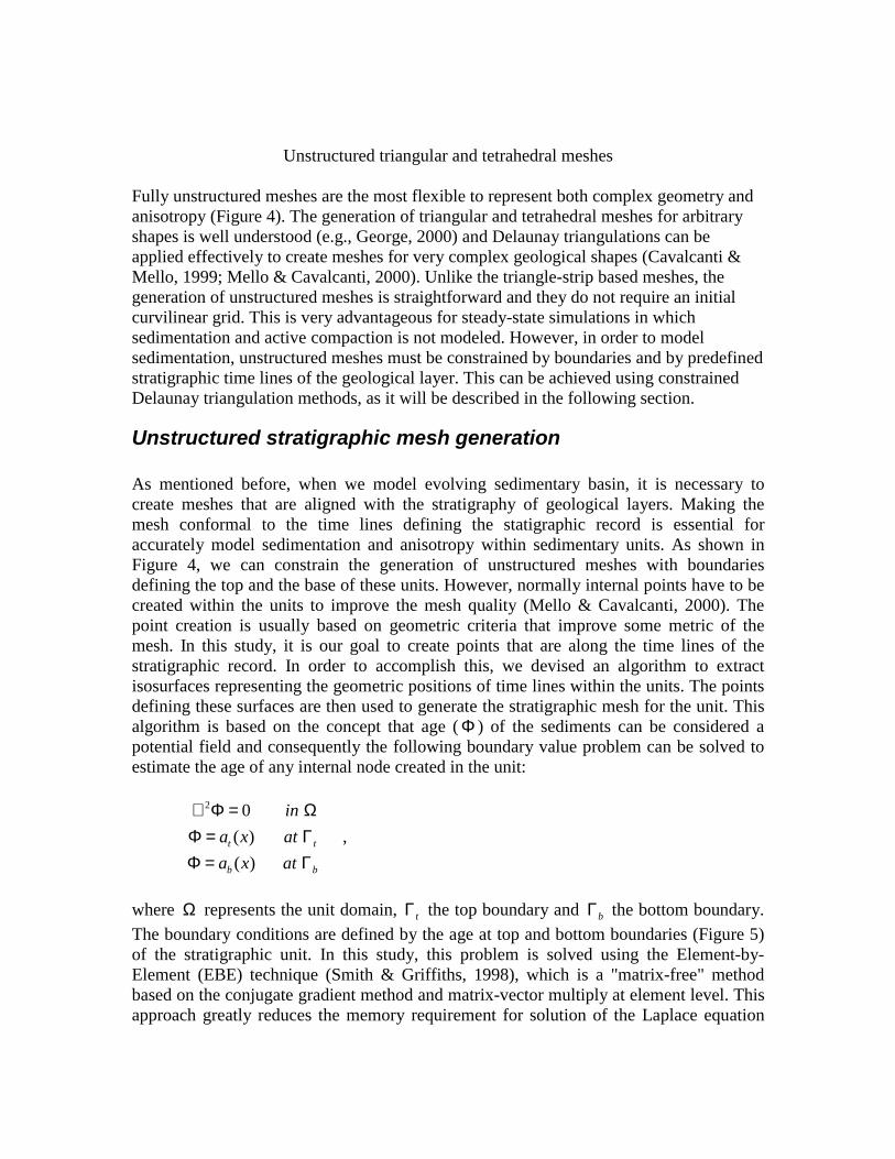
Unstructured stratigraphic mesh generation As mentioned before, when we model evolving sedimentary basin, it is necessary to create meshes that are aligned with the stratigraphy of geological layers. Making the mesh conformal to the time lines defining the statigraphic record is essential for accurately model sedimentation and anisotropy within sedimentary units. As shown in Figure 4, we can constrain the generation of unstructured meshes with boundaries defining the top and the base of these units. However, normally internal points have to be created within the units to improve the mesh quality (Mello & Cavalcanti, 2000). The point creation is usually based on geometric criteria that improve some metric of the mesh. In this study, it is our goal to create points that are along the time lines of the stratigraphic record. In order to accomplish this, we devised an algorithm to extract isosurfaces representing the geometric positions of time lines within the units. The points defining these surfaces are then used to generate the stratigraphic mesh for the unit. This algorithm is based on the concept that age ( Φ ) of the sediments can be considered a potential field and consequently the following boundary value problem can be solved to estimate the age of any internal node created in the unit:

2 0( )( )

t t

b b

in a x at a x at

∇ Φ = ΩΦ = ΓΦ = Γ

,

where Ω represents the unit domain, tΓ the top boundary and bΓ the bottom boundary. The boundary conditions are defined by the age at top and bottom boundaries (Figure 5) of the stratigraphic unit. In this study, this problem is solved using the Element-by-Element (EBE) technique (Smith & Griffiths, 1998), which is a "matrix-free" method based on the conjugate gradient method and matrix-vector multiply at element level. This approach greatly reduces the memory requirement for solution of the Laplace equation

because there is no need to assemble the global stiffness matrix. Only the storage of the element stiffness matrices is required. The algorithm to generate unstructured stratigraphic meshes follows the steps:

1. Select the stratigraphic unit to be subdivided; 2. Create a general mesh within the unit; 3. Define the ages on the top and bottom of the unit; 4. Solve the Laplace equation using Finite Elements (Zienkiewics & Taylor, 1989); 5. Generate isosurfaces defining time lines using a variation of the Marching cubes

algorithm for triangles or tetrahedra (Schroeder et al., 1997); 6. Insert the isosurfaces in the triangulation as internal boundaries; 7. Generate a Delaunay triangulation with internal boundaries as constrain

(Cavalcanti & Mello, 1999). A simple example of the application of this algorithm can be seen in Figures 6 and 7. In Figure 6, we started from a geological object representing a sigmoid geometry, typical of progradational sequences in deltaic depositional environments. For these examples, we assumed that the age at the top and bottom of the sigmoid were constant. After generating a general unstructured mesh, we solve the Laplace equation described before to find time lines (iso-ages). The time lines were then used to constrain the generation of a new mesh that contains these constraining lines. This technique is quite general and can be applied to regions with complex geometry. Figure 7 was generated in the same manner but in 3D. Note that in 3D, the definition of boundary conditions can be difficult to be accomplished automatically because the creation and maintenance of 3D models for basin modeling can be very complex (Mello & Henderson, 1997; Mello & Cavalcanti, in press). This algorithm has been implemented in MultiMesh Toolkit, which is described in detail in Mello & Cavalcanti (in press).

Compaction in unstructured meshes Before deriving the equations for compaction using unstructured meshes is useful to derive the equations to calculate the weight of the sediments, or the overburden lithostatic pressure, because these equations have the same characteristics of the compaction equations but they are simpler to understand.

Sediment overburden lithostatic pressure

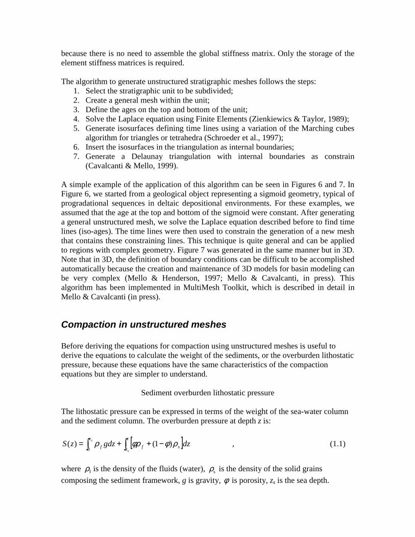
The lithostatic pressure can be expressed in terms of the weight of the sea-water column and the sediment column. The overburden pressure at depth z is:

[ ] −++=z

z sf

z

fs

s dzdzgzS ρφφρρ )1()(0

, (1.1)

where fρ is the density of the fluids (water), sρ is the density of the solid grains composing the sediment framework, g is gravity, φ is porosity, zs is the sea depth.

If the water density in the sea column is assumed to constant, the first integral of equation (1.1) can be integrated analytically:

[ ] −++=z

z sfsfs

dzgzzS ρφφρρ )1()( . (1.2)

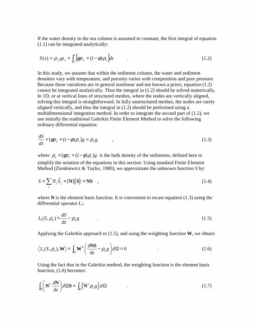
In this study, we assume that within the sediment column, the water and sediment densities vary with temperature, and porosity varies with composition and pore pressure. Because these variations are in general nonlinear and not known a priori, equation (1.2) cannot be integrated analytically. Thus the integral in (1.2) should be solved numerically. In 1D, or at vertical lines of structured meshes, where the nodes are vertically aligned, solving this integral is straightforward. In fully unstructured meshes, the nodes are rarely aligned vertically, and thus the integral in (1.2) should be performed using a multidimensional integration method. In order to integrate the second part of (1.2), we use initially the traditional Galerkin Finite Element Method to solve the following ordinary differential equation:

[ (1 ) ]f s adS g gdz

φρ φ ρ ρ= + − = , (1.3)

where [ (1 ) ]a f s gρ φρ φ ρ= + − is the bulk density of the sediments, defined here to simplify the notation of the equations in this section. Using standard Finite Element Method (Zienkiewicz & Taylor, 1989), we approximate the unknown function S by:

ˆ [ ]j jj

S N S= = = N S NS , (1.4)

where N is the element basis function. It is convenient to recast equation (1.3) using the differential operator L1:

1( , )ρ ρ= −a adSL S gdz

. (1.5)

Applying the Galerkin approach to (1.5), and using the weighting function W, we obtain:

1( , ), 0ρ ρΩ

= − Ω =

NSW WT

a adL S g ddz

. (1.6)

Using the fact that in the Galerkin method, the weighting function is the element basis function, (1.6) becomes:

( )ρΩ Ω

Ω = Ω

NN S NT T

ad d g ddz

. (1.7)

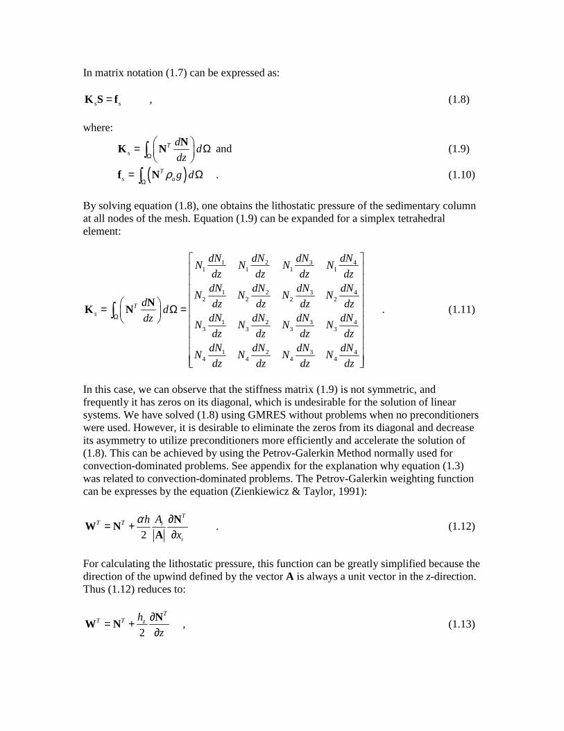
In matrix notation (1.7) can be expressed as:

s s=K S f , (1.8) where:

Ts

d ddzΩ

= Ω

NK N and (1.9)

( )ρΩ

= Ωf NTs a g d . (1.10)

By solving equation (1.8), one obtains the lithostatic pressure of the sedimentary column at all nodes of the mesh. Equation (1.9) can be expanded for a simplex tetrahedral element:

31 2 41 1 1 1

31 2 42 2 2 2

31 2 43 3 3 3

31 2 44 4 4 4

Ω

= Ω =

NK NT

s

dNdN dN dNN N N Ndz dz dz dz

dNdN dN dNN N N Nd dz dz dz dzd

dNdN dN dNdz N N N Ndz dz dz dz

dNdN dN dNN N N Ndz dz dz dz

. (1.11)

In this case, we can observe that the stiffness matrix (1.9) is not symmetric, and frequently it has zeros on its diagonal, which is undesirable for the solution of linear systems. We have solved (1.8) using GMRES without problems when no preconditioners were used. However, it is desirable to eliminate the zeros from its diagonal and decrease its asymmetry to utilize preconditioners more efficiently and accelerate the solution of (1.8). This can be achieved by using the Petrov-Galerkin Method normally used for convection-dominated problems. See appendix for the explanation why equation (1.3) was related to convection-dominated problems. The Petrov-Galerkin weighting function can be expresses by the equation (Zienkiewicz & Taylor, 1991):

2

TT T i

i

Ahx

α ∂= +∂NW N

A . (1.12)

For calculating the lithostatic pressure, this function can be greatly simplified because the direction of the upwind defined by the vector A is always a unit vector in the z-direction. Thus (1.12) reduces to:

2

TT T zh

z∂= +∂NW N , (1.13)

where zh is the element size in the z-direction. Applying (1.13) into (1.6), we obtain:

02

ρ ρΩ Ω

∂ − Ω = + − Ω = ∂

NS N NSW NT

T T za a

d h dg d g ddz z dz

, (1.14)

which expands to:

2 2ρ ρ

Ω Ω

∂ ∂+ Ω = + Ω ∂ ∂

N N N NN S NT T

T Tz za a

d h d hd g g ddz z dz z

. (1.15)

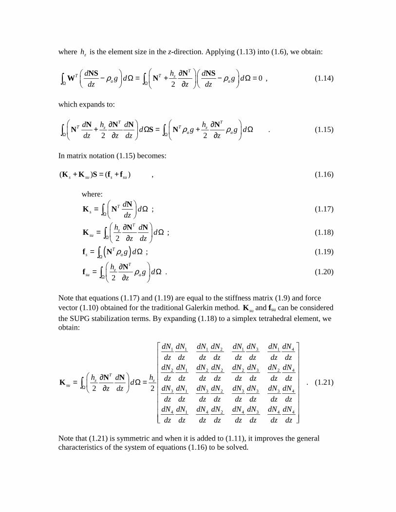
In matrix notation (1.15) becomes: ( ) ( )+ = +K K S f fs su s su , (1.16) where:

Ω

= Ω

NK NT

sd ddz

; (1.17)

2Ω

∂= Ω ∂

N NKT

zsu

h d dz dz

; (1.18)

( )ρΩ

= Ωf NTs a g d ; (1.19)

2ρ

Ω

∂= Ω ∂

NfT

zsu a

h g dz

. (1.20)

Note that equations (1.17) and (1.19) are equal to the stiffness matrix (1.9) and force vector (1.10) obtained for the traditional Galerkin method. suK and fsu can be considered the SUPG stabilization terms. By expanding (1.18) to a simplex tetrahedral element, we obtain:

31 1 1 2 1 1 4

32 1 2 2 2 2 4

3 3 3 3 31 2 4

34 1 4 2 4 4 4

2 2

Tz z

su

dNdN dN dN dN dN dN dNdz dz dz dz dz dz dz dz

dNdN dN dN dN dN dN dNh d h dz dz dz dz dz dz dz dzd

dN dN dN dN dNdN dN dNz dzdz dz dz dz dz dz dz dz

dNdN dN dN dN dN dN dNdz dz dz dz dz dz dz dz

Ω

∂= Ω = ∂

N NK

. (1.21)

Note that (1.21) is symmetric and when it is added to (1.11), it improves the general characteristics of the system of equations (1.16) to be solved.

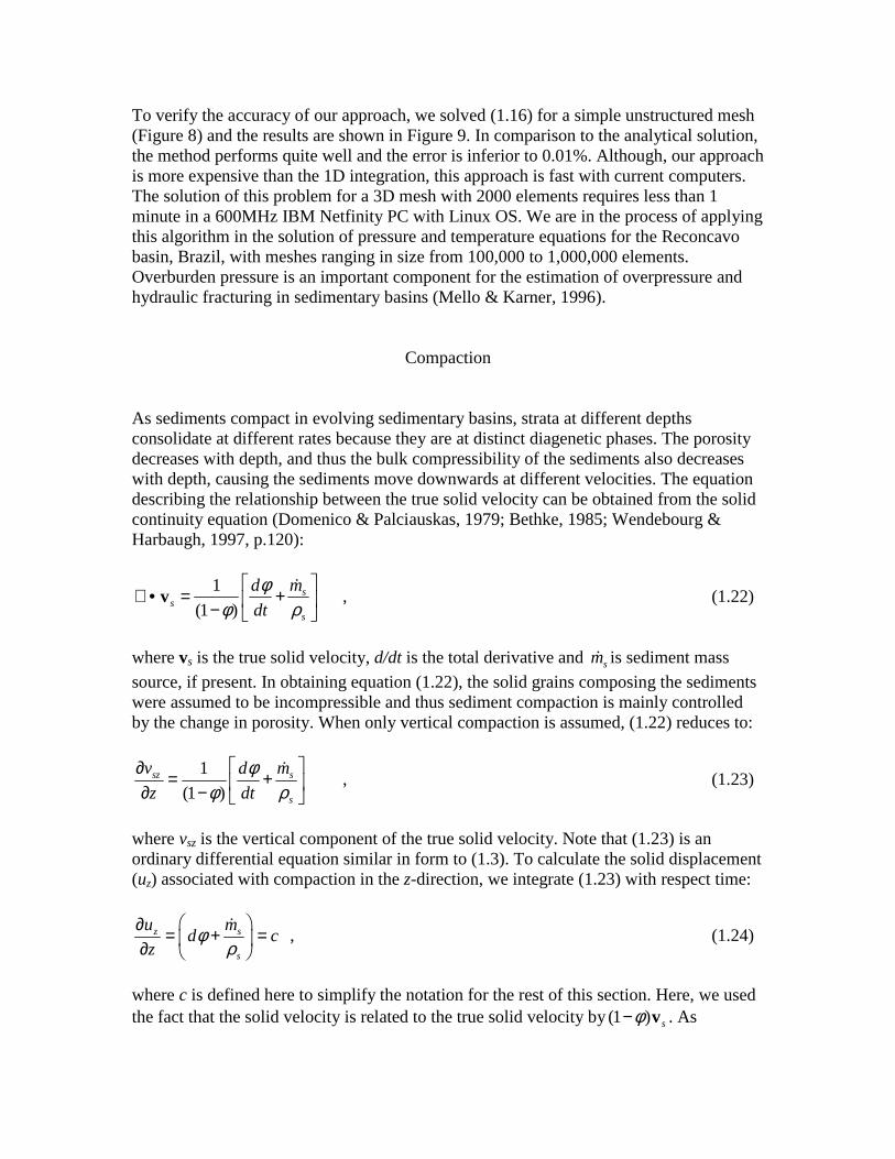
To verify the accuracy of our approach, we solved (1.16) for a simple unstructured mesh (Figure 8) and the results are shown in Figure 9. In comparison to the analytical solution, the method performs quite well and the error is inferior to 0.01%. Although, our approach is more expensive than the 1D integration, this approach is fast with current computers. The solution of this problem for a 3D mesh with 2000 elements requires less than 1 minute in a 600MHz IBM Netfinity PC with Linux OS. We are in the process of applying this algorithm in the solution of pressure and temperature equations for the Reconcavo basin, Brazil, with meshes ranging in size from 100,000 to 1,000,000 elements. Overburden pressure is an important component for the estimation of overpressure and hydraulic fracturing in sedimentary basins (Mello & Karner, 1996).

Compaction

As sediments compact in evolving sedimentary basins, strata at different depths consolidate at different rates because they are at distinct diagenetic phases. The porosity decreases with depth, and thus the bulk compressibility of the sediments also decreases with depth, causing the sediments move downwards at different velocities. The equation describing the relationship between the true solid velocity can be obtained from the solid continuity equation (Domenico & Palciauskas, 1979; Bethke, 1985; Wendebourg & Harbaugh, 1997, p.120):

1(1 )

φφ ρ

∇ • = + −

v s

ss

mddt

, (1.22)

where vs is the true solid velocity, d/dt is the total derivative and sm is sediment mass source, if present. In obtaining equation (1.22), the solid grains composing the sediments were assumed to be incompressible and thus sediment compaction is mainly controlled by the change in porosity. When only vertical compaction is assumed, (1.22) reduces to:

1(1 )

φφ ρ

∂ = + ∂ −

sz s

s

v mdz dt

, (1.23)

where vsz is the vertical component of the true solid velocity. Note that (1.23) is an ordinary differential equation similar in form to (1.3). To calculate the solid displacement (uz) associated with compaction in the z-direction, we integrate (1.23) with respect time:

φρ

∂ = + = ∂

sz

s

mu d cz

, (1.24)

where c is defined here to simplify the notation for the rest of this section. Here, we used the fact that the solid velocity is related to the true solid velocity by (1 )φ− vs . As

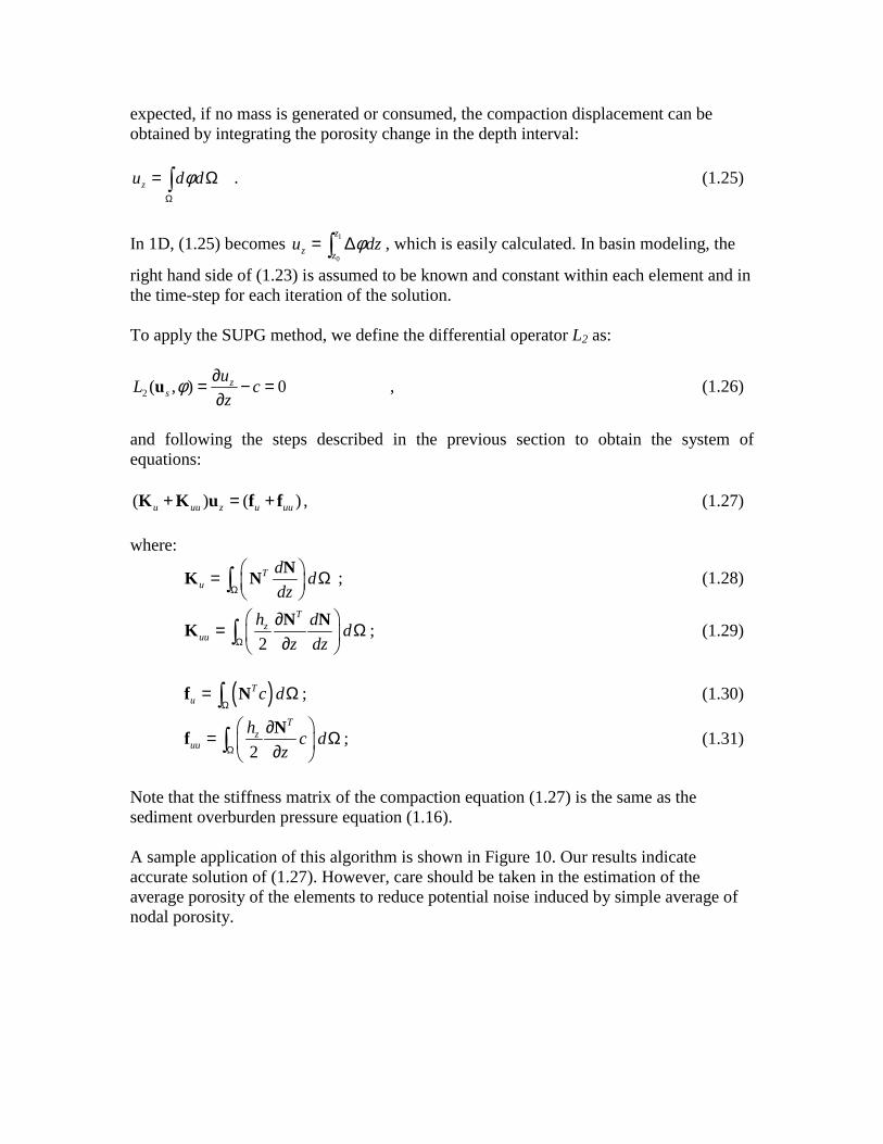
expected, if no mass is generated or consumed, the compaction displacement can be obtained by integrating the porosity change in the depth interval:

φΩ

= Ωzu d d . (1.25)

In 1D, (1.25) becomes 1

0φ= ∆

z

z zu dz , which is easily calculated. In basin modeling, the

right hand side of (1.23) is assumed to be known and constant within each element and in the time-step for each iteration of the solution. To apply the SUPG method, we define the differential operator L2 as:

2 ( , ) 0φ ∂= − =∂

u zs

uL cz

, (1.26)

and following the steps described in the previous section to obtain the system of equations: ( ) ( )+ = +K K u f fu uu z u uu , (1.27) where:

Ω

= Ω

NK NT

ud ddz

; (1.28)

2Ω

∂= Ω ∂

N NKT

zuu

h d dz dz

; (1.29)

( )

Ω= Ωf NT

u c d ; (1.30)

2Ω

∂= Ω ∂

NfT

zuu

h c dz

; (1.31)

Note that the stiffness matrix of the compaction equation (1.27) is the same as the sediment overburden pressure equation (1.16). A sample application of this algorithm is shown in Figure 10. Our results indicate accurate solution of (1.27). However, care should be taken in the estimation of the average porosity of the elements to reduce potential noise induced by simple average of nodal porosity.

Conclusions In this paper, we have presented techniques that fully exploit the characteristics of unstructured meshes in the modeling of evolving sedimentary basins in 2D and 3D. Unstructured meshes are more flexible than curvilinear grids and allow realistic representation of both complex geometry and anisotropy during the modeling. Realistic modeling is critical for using its results for prediction and risk assessment purposes. The techniques we described in this paper allow (1) the generation of stratigraphic meshes using Laplace equation to generate surfaces representing time lines that constrain the triangulation and (2) use a Streamline Upwind Finite Element formulation (SUPG) to calculate compaction during the simulation of evolving sedimentary basins. Although this paper has focused on basin modeling, many of the issues related to mesh generation discussed here are pertinent to other areas such as reservoir simulation. This is especially true nowadays, because of the need to incorporate more geological detail, anisotropy and complex well paths in reservoir simulations.

Acknowledgements This work was partially supported by Petrobrás and ENI-AGIP. P. R. Cavalcanti acknowledges the CNPq CTPETRO Grant # 468447/2000-8. We thank Gelonia Dent for reviewing this manuscript.

References Athy, L. F., 1930, Density, porosity, and compaction of sedimentary rocks, American Association of

Petroleum Geologists Bulletin, v.14:1-23. Bethke, C. M., 1985, A numerical model of compaction-driven groundwater flow and heat transfer and its

application to the paleohydrology of intracratonic sedimentary basins, Journal of Geophysical Research, v.90(B8):6817-6828.

Bitzer, K, 1996, Modeling consolidation and fluid flow in sedimentary basins, Computers & Geosciences,

v. 22(5):467-478. Burrus, J. and Audebert, F., 1990, Thermal and compaction processes in a young rifted basin containing

evaporates: Gulf of Lions, France, American Association of Petroleum Geologists Bulletin, v.74(9):1420-1440.

Cavalcanti, P. R. and Mello, U. T., 1999, Three-dimensional constrained Delaunay triangulation: a

minimalist approach, Proceedings of the 8th International Meshing Roundtable ’99, Lake Tahoe, CA, Oct. 10-13 1999, p. 119-129.

Domenico, P. A. and Palciauskas, V. V., 1979, Thermal expansion of fluids and fracture initiation in

compacting sediments, part II, Geological Society of America Bulletin, v. 90:953-979. George, P. L., 2000, Automatic mesh generation: application to finite element method, Hermes Science

Publications, 816pp.

Knupp, P. and Steinberg, S., 1993, Fundamentals of grid generation, CRC Press. Mello, U. T.; Karner, G. D. and Anderson, R. N., 1995, Role of salt in restraining the maturation of subsalt

source rocks, Marine and Petroleum Geology, v. 12(7):697-716. Mello, U. T. and Karner, G. D., 1996, Development of sediment overpressure and its effect on thermal

maturation: application to the Gulf of Mexico basin, American Association of Petroleum Geologists Bulletin, v. 80:1367-1396.

Mello, U. T. and Henderson, M. E., 1997, Techniques for including large deformations associated with salt

and fault motion in basin modeling, Marine and Petroleum Geology, v. 14(5):551-564. Mello, U. T. and Cavalcanti, P. R., 2000, A point creation strategy for mesh generation using crystal

lattices as templates, Proceedings of the 9th International Meshing Roundtable, New Orleans, Louisiana, Oct. 2000, p253-261.

Mello, U. T. and Cavalcanti, P. R., in press, A topologically-based framework for simulating complex

geological processes, AAPG Special Volume on the AAPG Hedberg Conference on Basin Modeling, Colorado Springs, Colorado, May 1999.

Person, M. and Garven, G., 1989, Hydrologic constraints on thermal evolution of the Rhine Graben, in

Beck, A. E; Garven, G.; Stegena, L., eds., , Hydrological regimes and their subsurface thermal effects: Geophysical Monograph 47, IUGG Volume 2, American Geophysical Union, p. 35-58.

Schroeder, W.; Martin, K. and Lorensen, B., 1997, The Visualization Toolkit : An object-oriented approach

to 3-D graphics, 2nd Edition, Prentice Hall Computer Books, 672p. Sclater, J. G. and Christie, P. A., 1980, Continental stretching: an explanation of post Mid-Cretaceous

subsidence of the central North Sea basin, Journal of Geophysical Research, v.85:3711-3739. Sharpe, H. N. and Anderson, D. A., 1990, Orthogonal curvilinear grid generation with preset internal

boundaries for reservoir simulation. SPE Paper 21235. Smith, I. M. and Griffiths, D. V., 1998, Programming the Finite Element Method, 3rd edition, John Wiley,

534p. Wendebourg, J. and Harbaugh, J. W., 1997, Simulating oil entrapment in clastic sequences (Computer

Methods in the Geosciences, v.16), Pergamon Press, 212p. Zienkiewicz, O. C. and Taylor, R. L., 1989, The finite element method, volume 1, 4th Edition, McGraw

Hill, 648p. Zienkiewicz, O. C.and Taylor, R. L., 1991, The finite element method, volume 2, McGraw Hill. Zienkiewicz, O. C.; Cheung, Y. K. & Stagg, K. G., 1966, Stresses in anysotropic media with particular

reference to problem of rock mechanics, Journal of Strain Analysis, V.1(2):172-182.

Appendix A convection-dominated process can be expressed, for example, by the equation:

T T Qdt∂ + • ∇ =v ,

where v is velocity, Q is the source term, t is time and T is the unknown quantity. In the steady-state it reduces to:

T Q• ∇ =v . If we assume that the velocity is non-zero only in the z-direction, it simplifies to:

zdTv Qdz

= .

Note that if vz is assumed to be equal the unit, this equation is an ODE with the same form of equations (1.3) and (1.24).

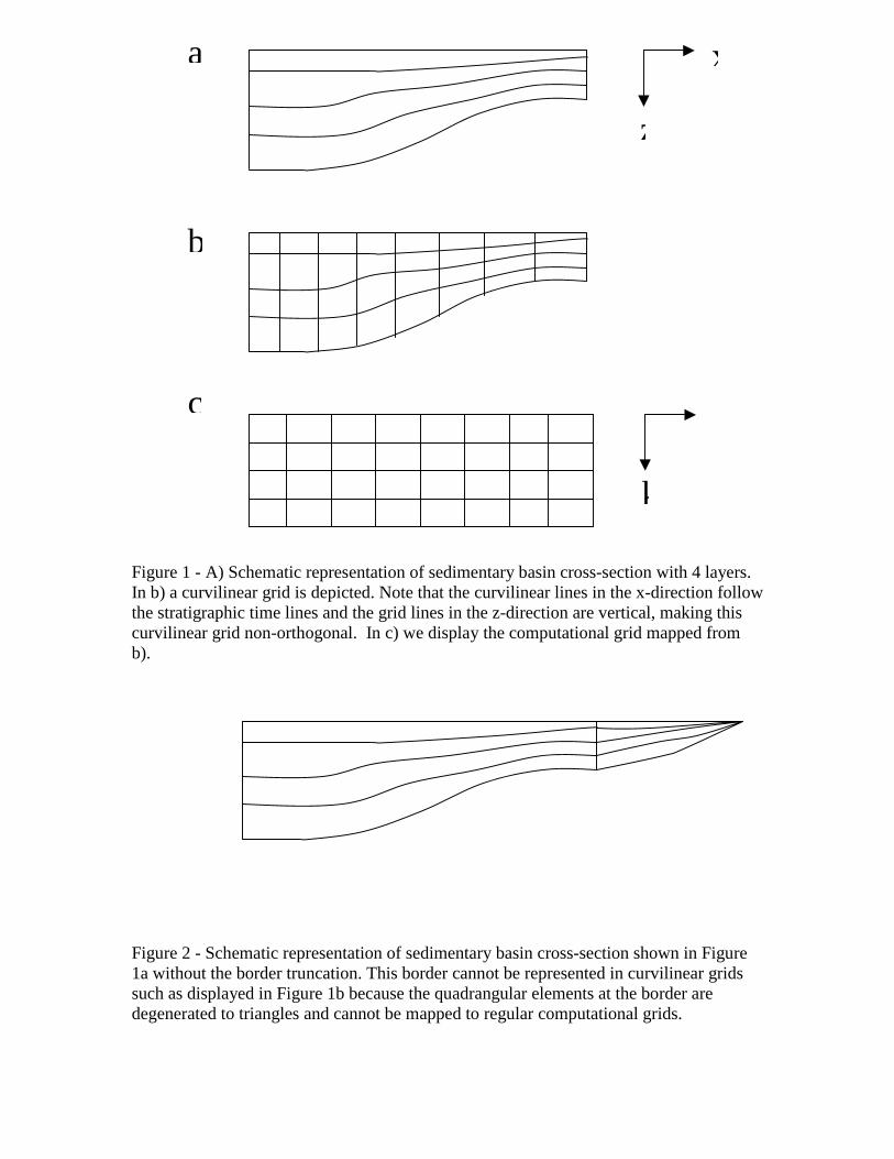
Figure 1 - A) Schematic representation of sedimentary basin cross-section with 4 layers. In b) a curvilinear grid is depicted. Note that the curvilinear lines in the x-direction follow the stratigraphic time lines and the grid lines in the z-direction are vertical, making this curvilinear grid non-orthogonal. In c) we display the computational grid mapped from b).

Figure 2 - Schematic representation of sedimentary basin cross-section shown in Figure 1a without the border truncation. This border cannot be represented in curvilinear grids such as displayed in Figure 1b because the quadrangular elements at the border are degenerated to triangles and cannot be mapped to regular computational grids.

x

z

a

b

c i

k

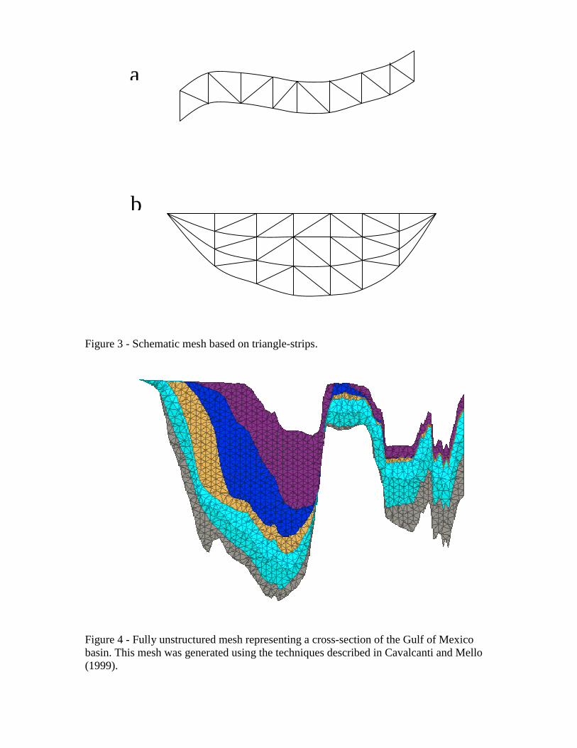
Figure 3 - Schematic mesh based on triangle-strips.

Figure 4 - Fully unstructured mesh representing a cross-section of the Gulf of Mexico basin. This mesh was generated using the techniques described in Cavalcanti and Mello (1999).

a

b

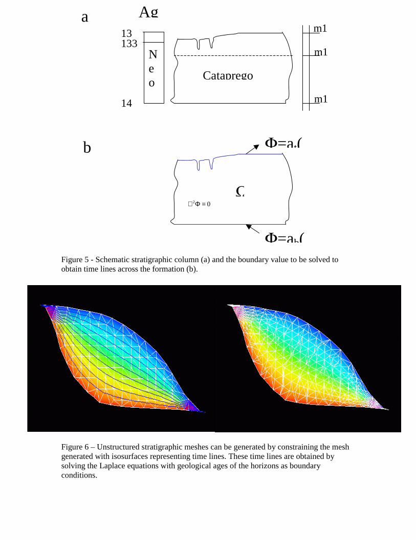
Figure 5 - Schematic stratigraphic column (a) and the boundary value to be solved to obtain time lines across the formation (b).

Figure 6 – Unstructured stratigraphic meshes can be generated by constraining the mesh generated with isosurfaces representing time lines. These time lines are obtained by solving the Laplace equations with geological ages of the horizons as boundary conditions.

m1

m1

m1

Neo

14

13133

Ag

Cataprego

=at(

=ab(

a

b

2 0∇ Φ =

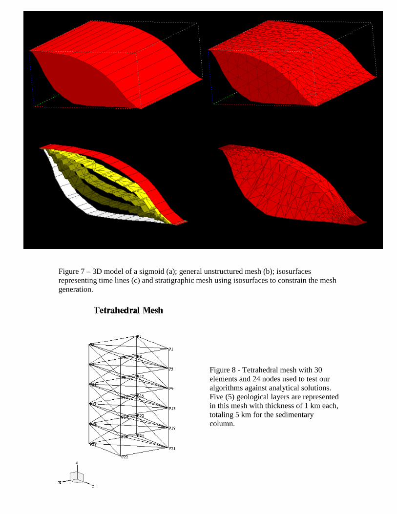
Figure 7 – 3D model of a sigmoid (a); general unstructured mesh (b); isosurfaces representing time lines (c) and stratigraphic mesh using isosurfaces to constrain the mesh generation.

Figure 8 - Tetrahedral mesh with 30 elements and 24 nodes used to test our algorithms against analytical solutions. Five (5) geological layers are represented in this mesh with thickness of 1 km each, totaling 5 km for the sedimentary column.

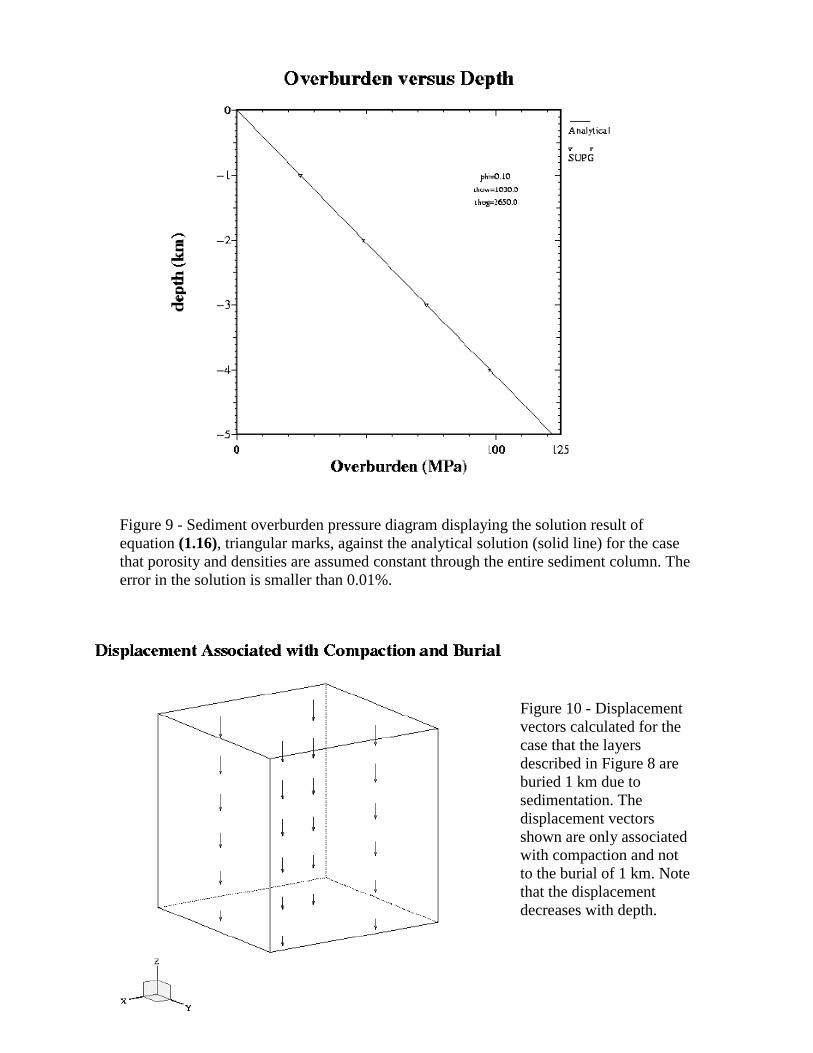
Figure 9 - Sediment overburden pressure diagram displaying the solution result of equation (1.16), triangular marks, against the analytical solution (solid line) for the case that porosity and densities are assumed constant through the entire sediment column. The error in the solution is smaller than 0.01%.

Figure 10 - Displacement vectors calculated for the case that the layers described in Figure 8 are buried 1 km due to sedimentation. The displacement vectors shown are only associated with compaction and not to the burial of 1 km. Note that the displacement decreases with depth.