Notes on S-PLUS - biostat.userweb.mwn.debiostat.userweb.mwn.de/teaching/compint2004/lit/splustutorial.pdfNotes on S-PLUS: A Programming Environment for Data Analysis and Graphics Bill

Notes on S-PLUS:

A Programming Environment for

Data Analysis and Graphics

Bill Venables and Dave Smith

Department of Statistics

The University of Adelaide

Email: [email protected]

c© W. Venables, 1990, 1992.

Version 2.2, September, 1992

Preface

These notes were originally intended only for local consumption at the University of Adelaide,South Australia. After some encouraging comments from students, the author decided to releasethem to a larger readership in the hope that in some small way they promote good data analysis. S

(or S-PLUS) is no panacea, of course, but in my view it represents the single complete environmentmost conducive to good data analysis so far available.

The authors are indebted to many people for useful contributions, but in particular Lucien W. VanElsen, who did the basic TEX to LaTEX conversion and Rick Becker who offered an authoritativeand extended critique on an earlier version. Others to offer useful comments and correctionsinclude Doug Bates, Ron Baxter, Ray Brownrigg, Sue Clancy, Kathy Haskard, Martin Maechler,James Pearce, Andreas Ruckstuhl and Catarina Savi.

Responsibility for this version, however, remains entirely with the authors, and the notes continueto enjoy a fully unofficial and unencumbered status.

These notes may be freely copied and redistributed provided the copyright notice remains intact.Where appropriate, a small charge to cover the costs of production and distribution, only, maybe made.

Comments and corrections are always welcome. Please address email correspondence to the firstauthor at [email protected].

Suggestions to the reader

Most S-PLUS novices will start with the introductory session in Appendix A. This should givesome familiarity with the style of S-PLUS sessions and more importantly some instant feedbackon what actually happens.

Many users will come to S-PLUS mainly for its graphical facilities. In this case section 11 onthe graphics facilities can be read at almost any time and need not wait until all the precedingsections have been digested.

Bill Venables and David Smith,University of Adelaide,6th September, 1992.

Contents

Preface

1 Introduction and Preliminaries 1

1.1 The S environment . . . . . . . . . . . . . . . . . . . . . . . . . . . . . . . . . . . 1

1.2 The S-PLUS environment . . . . . . . . . . . . . . . . . . . . . . . . . . . . . . . 1

1.3 Reference manuals . . . . . . . . . . . . . . . . . . . . . . . . . . . . . . . . . . . 1

1.4 S-PLUS and X–windows . . . . . . . . . . . . . . . . . . . . . . . . . . . . . . . . 1

1.5 Using S-PLUS interactively . . . . . . . . . . . . . . . . . . . . . . . . . . . . . . 2

1.6 An introductory session . . . . . . . . . . . . . . . . . . . . . . . . . . . . . . . . 2

1.7 S-PLUS and UNIX . . . . . . . . . . . . . . . . . . . . . . . . . . . . . . . . . . . 3

1.8 Getting help with functions and features . . . . . . . . . . . . . . . . . . . . . . . 3

1.9 S-PLUS commands. Case sensitivity. . . . . . . . . . . . . . . . . . . . . . . . . . 3

1.10 Recall and correction of previous commands . . . . . . . . . . . . . . . . . . . . . 4

1.10.1 S-PLUS . . . . . . . . . . . . . . . . . . . . . . . . . . . . . . . . . . . . . 4

1.10.2 S . . . . . . . . . . . . . . . . . . . . . . . . . . . . . . . . . . . . . . . . . 4

1.11 Executing commands from, or diverting output to, a file . . . . . . . . . . . . . . 4

1.12 Data directories. Permanency. Removing objects. . . . . . . . . . . . . . . . . . . 4

2 Simple manipulations; numbers and vectors 6

2.1 Vectors and Assignments . . . . . . . . . . . . . . . . . . . . . . . . . . . . . . . . 6

2.2 Vector arithmetic . . . . . . . . . . . . . . . . . . . . . . . . . . . . . . . . . . . . 6

2.3 Generating regular sequences . . . . . . . . . . . . . . . . . . . . . . . . . . . . . 7

2.4 Logical vectors . . . . . . . . . . . . . . . . . . . . . . . . . . . . . . . . . . . . . 8

2.5 Missing values . . . . . . . . . . . . . . . . . . . . . . . . . . . . . . . . . . . . . . 8

2.6 Character vectors . . . . . . . . . . . . . . . . . . . . . . . . . . . . . . . . . . . . 8

2.7 Index vectors. Selecting and modifying subsets of a data set . . . . . . . . . . . . 9

3 Objects, their modes and attributes 11

3.1 Intrinsic attributes: mode and length . . . . . . . . . . . . . . . . . . . . . . . . . 11

3.2 Changing the length of an object . . . . . . . . . . . . . . . . . . . . . . . . . . . 11

3.3 attributes() and attr() . . . . . . . . . . . . . . . . . . . . . . . . . . . . . . . 12

3.4 The class of an object . . . . . . . . . . . . . . . . . . . . . . . . . . . . . . . . . 12

4 Categories and factors 13

4.1 A specific example . . . . . . . . . . . . . . . . . . . . . . . . . . . . . . . . . . . 13

4.2 The function tapply() and ragged arrays . . . . . . . . . . . . . . . . . . . . . . 14

i

5 Arrays and matrices 15

5.1 Arrays . . . . . . . . . . . . . . . . . . . . . . . . . . . . . . . . . . . . . . . . . . 15

5.2 Array indexing. Subsections of an array . . . . . . . . . . . . . . . . . . . . . . . 15

5.3 Index arrays . . . . . . . . . . . . . . . . . . . . . . . . . . . . . . . . . . . . . . . 15

5.4 The array() function . . . . . . . . . . . . . . . . . . . . . . . . . . . . . . . . . 17

5.4.1 Mixed vector and array arithmetic. The recycling rule . . . . . . . . . . . 17

5.5 The outer product of two arrays . . . . . . . . . . . . . . . . . . . . . . . . . . . 17

5.5.1 An example: Determinants of 2 × 2 digit matrices . . . . . . . . . . . . . 18

5.6 Generalized transpose of an array . . . . . . . . . . . . . . . . . . . . . . . . . . . 18

5.7 Matrix facilities. Multiplication, inversion and solving linear equations. . . . . . . 19

5.8 Forming partitioned matrices. cbind() and rbind(). . . . . . . . . . . . . . . . 19

5.9 The concatenation function, c(), with arrays. . . . . . . . . . . . . . . . . . . . . 20

5.10 Frequency tables from factors. The table() function . . . . . . . . . . . . . . . . 20

6 Lists, data frames, and their uses 22

6.1 Lists . . . . . . . . . . . . . . . . . . . . . . . . . . . . . . . . . . . . . . . . . . . 22

6.2 Constructing and modifying lists . . . . . . . . . . . . . . . . . . . . . . . . . . . 22

6.2.1 Concatenating lists . . . . . . . . . . . . . . . . . . . . . . . . . . . . . . . 23

6.3 Some functions returning a list result . . . . . . . . . . . . . . . . . . . . . . . . . 23

6.3.1 Eigenvalues and eigenvectors . . . . . . . . . . . . . . . . . . . . . . . . . 23

6.3.2 Singular value decomposition and determinants . . . . . . . . . . . . . . . 23

6.3.3 Least squares fitting and the QR decomposition . . . . . . . . . . . . . . 24

6.4 Data frames . . . . . . . . . . . . . . . . . . . . . . . . . . . . . . . . . . . . . . . 24

6.4.1 Making data frames . . . . . . . . . . . . . . . . . . . . . . . . . . . . . . 25

6.4.2 attach() and detach() . . . . . . . . . . . . . . . . . . . . . . . . . . . . 25

6.4.3 Working with data frames . . . . . . . . . . . . . . . . . . . . . . . . . . . 25

6.4.4 Attaching arbitrary lists . . . . . . . . . . . . . . . . . . . . . . . . . . . . 26

7 Reading data from files 27

7.1 The read.table() function . . . . . . . . . . . . . . . . . . . . . . . . . . . . . . 27

7.2 The scan() function . . . . . . . . . . . . . . . . . . . . . . . . . . . . . . . . . . 27

7.3 Other facilities; editing data . . . . . . . . . . . . . . . . . . . . . . . . . . . . . . 28

8 More language features. Loops and conditional execution 29

8.1 Grouped expressions . . . . . . . . . . . . . . . . . . . . . . . . . . . . . . . . . . 29

8.2 Control statements . . . . . . . . . . . . . . . . . . . . . . . . . . . . . . . . . . . 29

8.2.1 Conditional execution: if statements . . . . . . . . . . . . . . . . . . . . 29

8.2.2 Repetitive execution: for loops, repeat and while . . . . . . . . . . . . . 29

ii

9 Writing your own functions 31

9.1 Simple examples . . . . . . . . . . . . . . . . . . . . . . . . . . . . . . . . . . . . 31

9.2 Defining new binary operators. . . . . . . . . . . . . . . . . . . . . . . . . . . . . 32

9.3 Named arguments and defaults. “. . . ” . . . . . . . . . . . . . . . . . . . . . . . . 32

9.4 Assignments within functions are local. Frames. . . . . . . . . . . . . . . . . . . . 33

9.5 More advanced examples . . . . . . . . . . . . . . . . . . . . . . . . . . . . . . . . 33

9.5.1 Efficiency factors in block designs . . . . . . . . . . . . . . . . . . . . . . . 33

9.5.2 Dropping all names in a printed array . . . . . . . . . . . . . . . . . . . . 34

9.5.3 Recursive numerical integration . . . . . . . . . . . . . . . . . . . . . . . . 35

9.6 Customising the environment. .First and .Last . . . . . . . . . . . . . . . . . . 35

9.7 Classes, generic functions and object orientation . . . . . . . . . . . . . . . . . . 36

10 Statistical models in S-PLUS 38

10.1 Defining statistical models; formulæ . . . . . . . . . . . . . . . . . . . . . . . . . 38

10.2 Regression models; fitted model objects . . . . . . . . . . . . . . . . . . . . . . . 40

10.3 Generic functions for extracting information . . . . . . . . . . . . . . . . . . . . . 40

10.4 Analysis of variance; comparing models . . . . . . . . . . . . . . . . . . . . . . . 40

10.4.1 ANOVA tables . . . . . . . . . . . . . . . . . . . . . . . . . . . . . . . . . 41

10.5 Updating fitted models. The ditto name “.” . . . . . . . . . . . . . . . . . . . . 42

10.6 Generalized linear models; families . . . . . . . . . . . . . . . . . . . . . . . . . . 42

10.6.1 Families . . . . . . . . . . . . . . . . . . . . . . . . . . . . . . . . . . . . . 43

10.6.2 The glm() function . . . . . . . . . . . . . . . . . . . . . . . . . . . . . . 43

10.7 Nonlinear regression models; parametrized data frames . . . . . . . . . . . . . . . 46

10.7.1 Changes to the form of the model formula . . . . . . . . . . . . . . . . . . 46

10.7.2 Specifying the parameters . . . . . . . . . . . . . . . . . . . . . . . . . . . 47

10.8 Some non-standard models . . . . . . . . . . . . . . . . . . . . . . . . . . . . . . 47

11 Graphical procedures 49

11.1 High-level plotting commands . . . . . . . . . . . . . . . . . . . . . . . . . . . . . 49

11.1.1 The plot() function . . . . . . . . . . . . . . . . . . . . . . . . . . . . . . 49

11.1.2 Displaying multivariate data . . . . . . . . . . . . . . . . . . . . . . . . . 50

11.1.3 Display graphics . . . . . . . . . . . . . . . . . . . . . . . . . . . . . . . . 50

11.1.4 Arguments to high-level plotting functions . . . . . . . . . . . . . . . . . . 51

11.2 Low-level plotting commands . . . . . . . . . . . . . . . . . . . . . . . . . . . . . 52

11.3 Interactive graphics functions . . . . . . . . . . . . . . . . . . . . . . . . . . . . . 53

11.4 Using graphics parameters . . . . . . . . . . . . . . . . . . . . . . . . . . . . . . . 54

11.4.1 Permanent changes: The par() function . . . . . . . . . . . . . . . . . . . 54

11.4.2 Temporary changes: Arguments to graphics functions . . . . . . . . . . . 55

iii

iv CONTENTS

11.5 Graphics parameters list . . . . . . . . . . . . . . . . . . . . . . . . . . . . . . . . 55

11.5.1 Graphical elements . . . . . . . . . . . . . . . . . . . . . . . . . . . . . . . 55

11.5.2 Axes and tick marks . . . . . . . . . . . . . . . . . . . . . . . . . . . . . . 56

11.5.3 Figure margins . . . . . . . . . . . . . . . . . . . . . . . . . . . . . . . . . 57

11.5.4 Multiple figure environment . . . . . . . . . . . . . . . . . . . . . . . . . . 58

11.6 Device drivers . . . . . . . . . . . . . . . . . . . . . . . . . . . . . . . . . . . . . . 59

11.6.1 PostScript diagrams for typeset documents. . . . . . . . . . . . . . . . . . 60

11.6.2 Multiple graphics devices . . . . . . . . . . . . . . . . . . . . . . . . . . . 60

A S-PLUS: An introductory session 62

B The Inbuilt Command Line Editor in S-PLUS 65

B.1 Preliminaries . . . . . . . . . . . . . . . . . . . . . . . . . . . . . . . . . . . . . . 65

B.2 Editing Actions . . . . . . . . . . . . . . . . . . . . . . . . . . . . . . . . . . . . . 65

B.3 Command Line Editor Summary . . . . . . . . . . . . . . . . . . . . . . . . . . . 66

C Exercises 67

C.1 The cloud point data . . . . . . . . . . . . . . . . . . . . . . . . . . . . . . . . . . 67

C.2 The Janka hardness data . . . . . . . . . . . . . . . . . . . . . . . . . . . . . . . 67

C.3 The Tuggeranong house price data . . . . . . . . . . . . . . . . . . . . . . . . . . 68

C.4 Yorke Penninsula wheat yield data . . . . . . . . . . . . . . . . . . . . . . . . . . 69

C.5 The Iowa wheat yield data . . . . . . . . . . . . . . . . . . . . . . . . . . . . . . . 70

C.6 The gasoline yield data . . . . . . . . . . . . . . . . . . . . . . . . . . . . . . . . 70

C.7 The Michaelson and Morley speed of light data . . . . . . . . . . . . . . . . . . . 72

C.8 The rat genotype data . . . . . . . . . . . . . . . . . . . . . . . . . . . . . . . . . 73

C.9 Fisher’s sugar beet data . . . . . . . . . . . . . . . . . . . . . . . . . . . . . . . . 74

C.10 A barley split plot field trial . . . . . . . . . . . . . . . . . . . . . . . . . . . . . . 75

C.11 The snail mortality data . . . . . . . . . . . . . . . . . . . . . . . . . . . . . . . . 76

C.12 The Kalythos blindness data . . . . . . . . . . . . . . . . . . . . . . . . . . . . . 77

C.13 The Stormer viscometer calibration data . . . . . . . . . . . . . . . . . . . . . . . 78

C.14 The chlorine availability data . . . . . . . . . . . . . . . . . . . . . . . . . . . . . 79

C.15 The saturated steam pressure data . . . . . . . . . . . . . . . . . . . . . . . . . . 79

C.16 Count Rumford’s friction data . . . . . . . . . . . . . . . . . . . . . . . . . . . . 80

C.17 The jellyfish data . . . . . . . . . . . . . . . . . . . . . . . . . . . . . . . . . . . . 81

C.18 The Archæological pottery data . . . . . . . . . . . . . . . . . . . . . . . . . . . . 81

C.19 The Beaujolais quality data . . . . . . . . . . . . . . . . . . . . . . . . . . . . . . 82

C.20 The painters data of de Piles . . . . . . . . . . . . . . . . . . . . . . . . . . . . . 83

Introduction and Preliminaries 1

1 Introduction and Preliminaries

1.1 The S environment

S is an integrated suite of software facilities for data manipulation, calculation and graphicaldisplay. Among other things it has

• an effective data handling and storage facility,

• a suite of operators for calculations on arrays, in particular matrices,

• a large, coherent, integrated collection of intermediate tools for data analysis,

• graphical facilities for data analysis and display either at a workstation or on hardcopy,and

• a well developed, simple and effective programming language which includes conditionals,loops, user defined recursive functions and input and output facilities. (Indeed most of thesystem supplied functions are themselves written in the S language.)

The term “environment” is intended to characterize it as a fully planned and coherent system,rather than an incremental accretion of very specific and inflexible tools, as is frequently the casewith other data analysis software.

S is very much a vehicle for newly developing methods of interactive data analysis. As such it isvery dynamic, and new releases have not always been fully upwardly compatible with previousreleases. Some users welcome the changes because of the bonus of new technology and newmethods that come with new releases; others seem to be more worried by the fact that old codeno longer works. Although S is intended as a programming language, in my view one shouldregard programs written in S as essentially ephemeral.

The name S as with many names within the UNIX world, is not explained, but left as a crypticpuzzle, and probably a weak pun. However its authors insist it does not stand for “Statistics”!

1.2 The S-PLUS environment

These notes will be mainly concerned with S-PLUS, an enhanced version of S distributed byStatistical Sciences, Inc., Seattle, Washington. Most of what we will have to say, however,applies interchangably to S and S-PLUS

1.3 Reference manuals

The basic reference is The New S Language: A Programming Environment for Data Analysis

and Graphics by Richard A. Becker, John M. Chambers and Allan R. Wilks. The new features ofthe August 1991 release of S are covered in Statistical Models in S Edited by John M. Chambersand Trevor J. Hastie. In addition there are specifically S-PLUS reference books: S-PLUS User’s

Manual (Volumes 1 & 2) and S-PLUS Reference Manual (in two volumes, A–K and L–Z).

It is not the intention of these notes to replace these manuals. Rather these notes are intendedas a brief introduction to the S-PLUS programming language and a minor amplification of someimportant points. Ultimately the user of S-PLUS will need to consult this reference manual,probably frequently.

1.4 S-PLUS and X–windows

The most convenient way to use S-PLUS is at a high quality graphics workstation running awindowing system. Since these are becoming more readily available, these notes are aimed at


users who have this facility. In particular we will occasionally refer to the use of S-PLUS on anX–window system, and even with the motif window manager, although the vast bulk of what issaid applies generally to any implementation of the S-PLUS environment.

Setting up a workstation to take full advantage of the customizable features of S-PLUS is astraightforward if somewhat tedious procedure, and will not be considered further here. Users indifficulty should seek local expert help.

1.5 Using S-PLUS interactively

When you use the S-PLUS program it issues a prompt when it expects input commands. Thedefault prompt is “>”, which is sometimes the same as the shell prompt, and so it may appearthat nothing is happening. However, as we shall see, it is easy to change to a different S-PLUS

prompt if you wish. In these notes we will assume that the shell prompt is “$ ”.

In using S-PLUS the suggested procedure for the first occasion is as follows:

1. Create a separate sub-directory, say work, to hold data files on which you will use S-PLUS

for this problem. This will be the working directory whenever you use S-PLUS for thisparticular problem.

$ mkdir work

$ cd work

2. Place any data files you wish to use with S-PLUS in work.

3. Create a sub-directory of work called .Data for use by S-PLUS.

$ mkdir .Data

4. Start the S-PLUS program editor with the command

$ Splus -e

(The -e flag is optional, but it allows the inbuilt line editor to be used, which is very handyfor correcting typing errors.)

5. At this point S-PLUS commands may be issued (see later).

6. To quit the S-PLUS program the command is

> q()

$

The procedure is simpler using S-PLUS after the first time:

Make work the working directory and start the program as before:

$ cd work

$ Splus -e

Use the S-PLUS program, terminating with the q() command at the end of the session.

1.6 An introductory session

Readers wishing to get a feel for S-PLUS at a workstation (or terminal) before proceeding arestrongly advised to work through the model introductory session given in Appendix A, startingon page 62.

1.7 S-PLUS and UNIX 3

1.7 S-PLUS and UNIX

S-PLUS allows escape to the operating system at any time in the session. If a command, on anew line, begins with an exclamation mark then the rest of the line is interpreted as a UNIX

command. So for example to look through a data file without leaving S-PLUS you could use

> !more curious.dat

When you finish paging the file the S-PLUS session is resumed.

In fact the integration of S-PLUS into UNIX is very complete. For example, there is a command,unix(. . .), that executes any unix command, (specified as a character string argument), andpasses on any output from the command as a character string to the program. Essentially thefull power of the operating system remains easily available to the user of the S-PLUS programduring any session.

The only non-UNIX implementation of S-PLUS so far is one for the DOS operating system. Usersshould consult the appropriate user guides for more information.

1.8 Getting help with functions and features

S-PLUS has an inbuilt help facility similar to the man facility of UNIX. To get more informationon any specific named function, for example solve the command is

> help(solve)

An alternative is

> ?solve

For a feature specified by special characters, the argument must be enclosed in double or singlequotes, making it a ‘character string’:

> help("[[")

Either form of quote mark may be used to escape the other, as in the string "It’s important".Our convention in these notes is to use double quote marks for preference.

A much more comprehensive help facility is available with the X windows version of S-PLUS Thecommand

> help.start(gui="motif")

causes a “help window” to appear (with the “motif” graphical user interface). It is at this pointpossible to select items interactively from a series of menus, and the selection process again causesother windows to appear with the help information. This may be either scanned at the screenand dismissed, or sent to a printer for hardcopy, or both.

1.9 S-PLUS commands. Case sensitivity.

Technically S-PLUS is a function language with a very simple syntax. It is case sensitive as aremost UNIX based packages, so A and a are different variables.

Elementary commands consist of either expressions or assignments. If an expression is givenas a command, it is evaluated, printed, and the value is lost. An assignment also evaluates anexpression and passes the value to a variable but the result is not automatically printed.

Commands are separated either by a semi-colon, ;, or by a newline. If a command is not completeat the end of a line, S-PLUS will give a different prompt, for example

+


on second and subsequent lines and continue to read input until the command is syntacticallycomplete. This prompt may also be changed if the user wishes. In these notes we will generallyomit the continuation prompt and indicate continuation by simple indenting.

1.10 Recall and correction of previous commands

1.10.1 S-PLUS

S-PLUS (but not plain S) provides a mechanism for recall and correction of previous commands.For interactive use this is a vital facility and greatly increases the productive output of mostpeople. To invoke S-PLUS with the command recall facility enabled use the -e flag:

> Splus -e

Within the session, command recall is available using either emacs-style or vi-style commands.The former is very similar to command recall with an interactive shell such as tcsh. Details aregiven in Appendix B of these notes, or they may be found in the reference manual or the onlinehelp documents.

1.10.2 S

With S no built-in mechanism is available, but there are two common ways of obtaining commandrecall for interactive sessions.

• Run the S session under emacs using S–mode, a major mode designed to support S. This isprobably more convenient than even the inbuilt editor of S-PLUS in the long term, howeverit does require a good deal of preliminary effort for persons not familiar with the emacs

editor. It also often requires a dedicated workstation with a good deal of memory and otherresources.

• Run the S session under some front end processor, such as the public domain fep program,available from the public sources archives. This provides essentially the same service as theinbuilt S-PLUS editor, but with somewhat more overhead, (but a great deal less overheadthan emacs requires.)

1.11 Executing commands from, or diverting output to, a file

If commands are stored on an external file, say commands.S in the working directory work, theymay be executed at any time in an S-PLUS session with the command

> source("commands.S")

Similarly

> sink("record.lis")

will divert all subsequent output from the terminal to an external file, record.lis. The command

> sink()

restores it to the terminal once again.

1.12 Data directories. Permanency. Removing objects.

The entities that S-PLUS creates and manipulates are known as objects. These may be vari-ables, arrays of numbers, character strings, functions, or more general structures built from suchcomponents.

1.12 Data directories. Permanency. Removing objects. 5

All objects created during your S-PLUS sessions are stored as files, in a special form, in the .Datasub-directory of your working directory work, say.

Each object is held as a separate file of the same name and so may be manipulated by the usualUNIX commands such as rm, cp and mv. This means that if you resume your S-PLUS session ata later time, objects created in previous sessions are still available, which is a highly convenientfeature.

This also explains why it is recommended that you should use separate working directories fordifferent jobs. Common names for objects are single letter names like x, y and so on, and if twoproblems share the same .Data sub-directory the objects will become mixed up and you mayoverwrite one with another.

There is, however, another method of partitioning variables within the same .Data directoryusing data frames. These are discussed further in §6.4.

In S-PLUS, to get a list of names of the objects currently defined use the command

> objects()

whose result is a vector of character strings giving the names.

When S-PLUS looks for an object, it searches in turn through a sequence of places known as thesearch list. Usually the first entry in the search list is the .Data sub-directory of the currentworking directory. The names of the places currently on the search list are displayed by thefunction

> search()

The names of the objects held in any place in the search list can be displayed by giving theobjects() function an argument. For example

> objects(2)

lists the contents of the entity at position 2 of the search list. The search list can contain eitherdata frames and allies, which are themselves internal S-PLUS objects, as well as directories offiles which are UNIX objects.

Extra entities can be added to this list with the attach() function and removed with thedetach() function, details of which can be found in the manual or the help facility.

To remove objects permanently the function rm is available:

> rm(x, y, z, ink, junk, temp, foo, bar)

The function remove() can be used to remove objects with non-standard names. Also theordinary UNIX facility, rm, may be used to remove the appropriate files in the .Data directory,as mentioned above.

6 Simple manipulations; numbers and vectors


2.1 Vectors and Assignments

S-PLUS operates on named data structures. The simplest such structure is the vector, which isa single entity consisting of an ordered collection of numbers. To set up a vector named x, say,consisting of five numbers, namely 10.4, 5.6, 3.1, 6.4 and 21.7, use the S-PLUS command

> x <- c(10.4, 5.6, 3.1, 6.4, 21.7)

This is an assignment statement using the function c() which in this context can take an arbitrarynumber of vector arguments and whose value is a vector got by concatenating its arguments endto end.1

A number occurring by itself in an expression is taken as a vector of length one.

Notice that the assignment operator is not the usual = operator, which is reserved for anotherpurpose. It consists of the two characters < (‘less than’) and - (‘minus’) occurring strictly side-by-side and it ‘points’ to the object receiving the value of the expression.2

Assignments can also be made in the other direction, using the obvious change in the assignmentoperator. So the same assignment could be made using

> c(10.4, 5.6, 3.1, 6.4, 21.7) -> x

If an expression is used as a complete command, the value is printed and lost. So now if we wereto use the command

> 1/x

the reciprocals of the five values would be printed at the terminal (and the value of x, of course,unchanged).

The further assignment

> y <- c(x, 0, x)

would create a vector y with 11 entries consisting of two copies of x with a zero in the middleplace.

2.2 Vector arithmetic

Vectors can be used in arithmetic expressions, in which case the operations are performed elementby element. Vectors occurring in the same expression need not all be of the same length. If theyare not, the value of the expression is a vector with the same length as the longest vector whichoccurs in the expression. Shorter vectors in the expression are recycled as often as need be(perhaps fractionally) until they match the length of the longest vector. In particular a constantis simply repeated. So with the above assignments the command

> v <- 2*x + y + 1

generates a new vector v of length 11 constructed by adding together, element by element, 2*xrepeated 2.2 times, y repeated just once, and 1 repeated 11 times.

The elementary arithmetic operators are the usual +, -, *, / and ^ for raising to a power. Inaddition all of the common arithmetic functions are available. log, exp, sin, cos, tan, sqrt, andso on, all have their usual meaning. max and min select the largest and smallest elements of anvector respectively. range is a function whose value is a vector of length two, namely c(min(x),

1With other than vector types of argument, such as list mode arguments, the action of c() is rather different.See §6.2.1.

2The underscore character, “ ” is an allowable synonym for the left pointing assignment operator “<-”, howeverwe discourage this option, as it can easily lead to much less readible code.

2.3 Generating regular sequences 7

max(x)). length(x) is the number of elements in x, sum(x) gives the total of the elements in x

and prod(x) their product.

Two statistical functions are mean(x) which calculates the sample mean, which is the same assum(x)/length(x), and var(x) which gives

sum((x-mean(x))^2)/(length(x)-1)

or sample variance. If the argument to var() is an n × p matrix the value is a p × p samplecovariance matrix got by regarding the rows as independent p−variate sample vectors.

sort(x) returns a vector of the same size as x with the elements arranged in increasing order;however there are other more flexible sorting facilities available (see order() or sort.list()

which produce a permutation to do the sorting).

rnorm(x) is a function which generates a vector (or more generally an array) of pseudo-randomstandard normal deviates, of the same size as x.

2.3 Generating regular sequences

S-PLUS has a number of facilities for generating commonly used sequences of numbers. Forexample 1:30 is the vector c(1,2, . . . ,29,30). The colon operator has highest priority withinan expression, so, for example 2*1:15 is the vector c(2,4,6, . . . ,28,30). Put n <- 10 andcompare the sequences 1:n-1 and 1:(n-1).

The construction 30:1 may be used to generate a sequence backwards.

The function seq() is a more general facility for generating sequences. It has five arguments,only some of which may be specified in any one call. The first two arguments, if given, specifythe beginning and end of the sequence, and if these are the only two arguments given the resultis the same as the colon operator. That is seq(2,10) is the same vector as 2:10.

Parameters to seq(), and to many other S-PLUS functions, can also be given in named form,in which case the order in which they appear is irrelevant. The first two parameters maybe named from=value and to=value; thus seq(1,30), seq(from=1, to=30) and seq(to=30,

from=1) are all the same as 1:30. The next two parameters to seq() may be named by=value

and length=value, which specify a step size and a length for the sequence respectively. If neitherof these is given, the default by=1 is assumed.

For example

> seq(-5, 5, by=.2) -> s3

generates in s3 the vector c(-5.0, -4.8, -4.6, . . ., 4.6, 4.8, 5.0). Similarly

> s4 <- seq(length=51, from=-5, by=.2)

generates the same vector in s4.

The fifth parameter may be named along=vector, which if used must be the only parameter, andcreates a sequence 1, 2, . . . , length(vector), or the empty sequence if the vector is empty (asit can be).

A related function is rep() which can be used for replicating an object in various complicatedways. The simplest form is

> s5 <- rep(x, times=5)

which will put five copies of x end-to-end in s5.


2.4 Logical vectors

As well as numerical vectors, S-PLUS allows manipulation of logical quantities. The elements ofa logical vectors have just two possible values, represented formally as F (for ‘false’) and T (for‘true’).

Logical vectors are generated by conditions. For example

> temp <- x>13

sets temp as a vector of the same length as x with values F corresponding to elements of x wherethe condition is not met and T where it is.

The logical operators are <, <=, >, >=, == for exact equality and != for inequality. In additionif c1 and c2 are logical expressions, then c1 & c2 is their intersection, c1 | c2 is their union and! c1 is the negation of c1.

Logical vectors may be used in ordinary arithmetic, in which case they are coerced into numericvectors, F becoming 0 and T becoming 1. However there are situations where logical vectors andtheir coerced numeric counterparts are not equivalent, for example see the next subsection.

2.5 Missing values

In some cases the components of a vector may not be completely known. When an elementor value is “not available” or a “missing value” in the statistical sense, a place within a vectormay be reserved for it by assigning it the special value NA. In general any operation on an NA

becomes an NA. The motivation for this rule is simply that if the specification of an operation isincomplete, the result cannot be known and hence is not available.

The function is.na(x) gives a logical vector of the same size as x with value T if and only if thecorresponding element in x is NA.

> ind <- is.na(z)

Notice that the logical expression x == NA is quite different from is.na(x) since NA is not reallya value but a marker for a quantity that is not available. Thus x == NA is a vector of the samelength as x all of whose values are NA as the logical expression itself is incomplete and henceundecidable.

2.6 Character vectors

Character quantities and character vectors are used frequently in S-PLUS, for example as plotlabels. Where needed they are denoted by a sequence of characters delimited by the double quotecharacter. E. g. "x-values", "New iteration results".

Character vectors may be concatenated into a vector by the c() function; examples of their usewill emerge frequently.

The paste() function takes an arbitrary number of arguments and concatenates them into asingle character string. Any numbers given among the arguments are coerced into characterstrings in the evident way, that is, in the same way they would be if they were printed. Thearguments are by default separated in the result by a single blank character, but this can bechanged by the named parameter, sep=string , which changes it to string , possibly empty.

For example

> labs <- paste(c("X","Y"), 1:10, sep="")

makes labs into the character vector

("X1", "Y2", "X3", "Y4", "X5", "Y6", "X7", "Y8", "X9", "Y10")

2.7 Index vectors. Selecting and modifying subsets of a data set 9

Note particularly that recycling of short lists takes place here too; thus c("X", "Y") is repeated5 times to match the sequence 1:10.

2.7 Index vectors. Selecting and modifying subsets of a data set

Subsets of the elements of a vector may be selected by appending to the name of the vector anindex vector in square brackets. More generally any expression that evaluates to a vector mayhave subsets of its elements similarly selected by appending an index vector in square bracketsimmediately after the expression.

Such index vectors can be any of four distinct types.

1. A logical vector. In this case the index vector must be of the same length as the vectorfrom which elements are to be selected. Values corresponding to T in the index vector areselected and those corresponding to F omitted. For example

> y <- x[!is.na(x)]

creates (or re-creates) an object y which will contain the non-missing values of x, in thesame order. Note that if x has missing values, y will be shorter than x. Also

> (x+1)[(!is.na(x)) & x>0] -> z

creates an object z and places in it the values of the vector x+1 for which the correspondingvalue in x was both non-missing and positive.

2. A vector of positive integral quantities. In this case the values in the index vector mustlie in the the set {1, 2, . . . , length(x)}. The corresponding elements of the vector areselected and concatenated, in that order, in the result. The index vector can be of anylength and the result is of the same length as the index vector. For example x[6] is thesixth component of x and

> x[1:10]

selects the first 10 elements of x, (assuming length(x) ≥ 10). Also

> c("x","y")[rep(c(1,2,2,1), times=4)]

(an admittedly unlikely thing to do) produces a character vector of length 16 consisting of"x", "y", "y", "x" repeated four times.

3. A vector of negative integral quantities. Such an index vector specifies the values to beexcluded rather than included. Thus

> y <- x[-(1:5)]

gives y all but the first five elements of x.

4. A vector of character strings. This possibility only applies where an object has a names

attribute to identify its components. In this case a subvector of the names vector may beused in the same way as the positive integral labels in 2. above.

> fruit <- c(5, 10, 1, 20)

> names(fruit) <- c("orange", "banana", "apple", "peach")

> lunch <- fruit[c("apple","orange")]

The advantage is that alphanumeric names are often easier to remember than numeric

indices. This option is particularly useful in connection with data frames, as we shall seelater.

An indexed expression can also appear on the receiving end of an assignment, in which case theassignment operation is performed only on those elements of the vector. The expression must be


of the form vector[index vector] as having an arbitrary expression in place of the vector namedoes not make much sense here.

The vector assigned must match the length of the index vector, and in the case of a logical indexvector it must again be the same length as the vector it is indexing.

For example

> x[is.na(x)] <- 0

replaces any missing values in x by zeros and

> y[y<0] <- -y[y<0]

has the same effect as

> y <- abs(y)3

3Note that abs() does not work as expected with complex arguments. The appropriate function for the complexmodulus is Mod().

Objects, their modes and attributes 11

3 Objects, their modes and attributes

3.1 Intrinsic attributes: mode and length

The entities S-PLUS operates on are technically known as objects. Examples are vectors ofnumeric (real) or complex values, vectors of logical values and vectors of character strings. Theseare known as ‘atomic’ structures since their components are all of the same type, or mode, namelynumeric4, complex, logical and character respectively.

Vectors must have their values all of the same mode. Thus any given vector must be unambigu-ously either logical, numeric, complex or character. The only mild exception to this rule is thespecial “value” listed as NA for quantities not available. Note that a vector can be empty andstill have a mode. For example the empty character string vector is listed as character(0) andthe empty numeric vector as numeric(0).

S-PLUS also operates on objects called lists, which are of mode list. These are ordered sequencesof objects which individually can be of any mode. lists are known as ‘recursive’ rather thanatomic structures since their components can themselves be lists in their own right.

The other recursive structures are those of mode function and expression. Functions are thefunctions that form part of the S-PLUS system along with similar user written functions, whichwe discuss in some detail later in these notes. Expressions as objects form an advanced part ofS-PLUS which will not be discussed in these notes, except indirectly when we discuss formulæ

used with modelling in S-PLUS.

By the mode of an object we mean the basic type of its fundamental constituents. This is a specialcase of an attribute of an object. The attributes of an object provide specific information aboutthe object itself. Another attribute of every object is its length. The functions mode(object) andlength(object) can be used to find out the mode and length of any defined structure.

For example, if z is a complex vector of length 100, then in an expression mode(z) is the characterstring "complex" and length(z) is 100.

S-PLUS caters for changes of mode almost anywhere it could be considered sensible to do so,(and a few where it might not be). For example with

> z <- 0:9

we could put

> digits <- as.character(z)

after which digits is the character vector ("0", "1", "2", . . ., "9"). A further coercion, orchange of mode, reconstructs the numerical vector again:

> d <- as.numeric(digits)

Now d and z are the same.5 There is a large collection of functions of the form as.something()

for either coercion from one mode to another, or for investing an object with some other attributeit may not already possess. The reader should consult the help file to become familiar with them.

3.2 Changing the length of an object

An “empty” object may still have a mode. For example

> e <- numeric()

4numeric mode is actually an amalgam of three distinct modes, namely integer, single precision and double

precision, as explained in the manual.5In general coercion from numeric to character and back again will not be exactly reversible, because of roundoff

errors in the character representation.

12 Objects, their modes and attributes

makes e an empty vector structure of mode numeric. Similarly character() is a empty charactervector, and so on. Once an object of any size has been created, new components may be addedto it simply by giving it an index value outside its previous range. Thus

> e[3] <- 17

now makes e a vector of length 3, (the first two components of which are at this point both NA).This applies to any structure at all, provided the mode of the additional component(s) agreeswith the mode of the object in the first place.

This automatic adjustment of lengths of an object is used often, for example in the scan()

function for input. (See §7.2.)

Conversely to truncate the size of an object requires only an assignment to do so. Hence if alphais an object of length 10, then

> alpha <- alpha[2 * 1:5]

makes it an object of length 5 consisting of just the former components with even index. Theold indices are not retained, of course.

3.3 attributes() and attr()

The function attributes(object) gives a list of all the non-intrinsic attributes currently definedfor that object. The function attr(object,name) can be used to select a specific attribute.These functions are rarely used, except in rather special circumstances when some new attributeis being created for some particular purpose, for example to associate a creation date or anoperator with an S-PLUS object. The concept, however, is very important.

3.4 The class of an object

A special attribute known as the class of the object has been introduced in the August 1991release of S and S-PLUS to allow for an object oriented style of programming in S-PLUS.

For example if an object has class data.frame, it will be printed in a certain way, the plot()

function will display it graphically in a certain way, and other generic functions such as summary()will react to it as an argument in a way sensitive to its class.

To remove temporarily the effects of class, use the function unclass(). For example if winterhas the class data.frame then

> winter

will print it in data frame form, which is rather like a matrix, whereas

> unclass(winter)

will print it as an ordinary list. Only in rather special situations do you need to use this facility,but one is when you are learning to come to terms with the idea of class and generic functions.

Generic functions and classes will be discussed further in §9.7, but only briefly.

Categories and factors 13

4 Categories and factors

A category is a vector object used to specify a discrete classification of the components of othervectors of the same length. A factor is similar, but has the class factor, which means that itis adapted to the generic function mechanism. Whereas a category can also be used as a plainnumeric vector, for example, a factor generally cannot.

4.1 A specific example

Suppose, for example, we have a sample of 30 tax accountants from the all states and territories6

and their individual state of origin is specified by a character vector of state mnemonics as

> state <- c("tas", "sa", "qld", "nsw", "nsw", "nt", "wa", "wa",

"qld", "vic", "nsw", "vic", "qld", "qld", "sa", "tas",

"sa", "nt", "wa", "vic", "qld", "nsw", "nsw", "wa",

"sa", "act", "nsw", "vic", "vic", "act")

For some purposes it is convenient to represent such information by a numeric vector with thedistinct values in the original (in this case the state labels) represented by a small integer. Sucha numeric vector is called a category. However at the same time it is important to preserve thecorrespondence of these new integer labels with the originals. This is done via the levels attributeof the category.

More formally, when a category is formed from such a vector the sorted unique values in thevector form the levels attribute of the category, and the values in the category are in the set 1,2, . . ., k where k is the number of unique values. The value at position j in the factor is i ifthe ith sorted unique value occurred at position j of the original vector.

Hence the assignment

> stcode <- category(state)

creates a category with values and attributes as follows

> stcode

[1] 6 5 4 2 2 3 8 8 4 7 2 7 4 4 5 6 5 3 8 7 4 2 2 8 5 1 2 7 7 1

attr(, "levels"):

[1] "act" "nsw" "nt" "qld" "sa" "tas" "vic" "wa"

Notice that in the case of a character vector, “sorted” means sorted in alphabetical order.

A factor is similarly created using the factor() function:

> statef <- factor(state)

The print() function now handles the factor object slightly differently:

> statef

[1] tas sa qld nsw nsw nt wa wa qld vic nsw vic qld qld sa

[16] tas sa nt wa vic qld nsw nsw wa sa act nsw vic vic act

If we remove the factor class, however, using the function unclass(), it becomes virtually iden-tical to the category:

> unclass(statef)

[1] 6 5 4 2 2 3 8 8 4 7 2 7 4 4 5 6 5 3 8 7 4 2 2 8 5 1 2 7 7 1

attr(, "levels"):

[1] "act" "nsw" "nt" "qld" "sa" "tas" "vic" "wa"

6Foreign readers should note that there are eight states and territories in Australia, namely the AustralianCapital Territory, New South Wales, the Northern Territory, Queensland, South Australia, Tasmania, Victoriaand Western Australia.

14 Categories and factors

4.2 The function tapply() and ragged arrays

To continue the previous example, suppose we have the incomes of the same tax accountants inanother vector (in suitably large units of money)

> incomes <- c(60, 49, 40, 61, 64, 60, 59, 54, 62, 69, 70, 42, 56,

61, 61, 61, 58, 51, 48, 65, 49, 49, 41, 48, 52, 46,

59, 46, 58, 43)

To calculate the sample mean income for each state we can now use the special function tapply():

> incmeans <- tapply(incomes, statef, mean)

giving a means vector with the components labelled by the levels

> incmeans

act nsw nt qld sa tas vic wa

44.5 57.333 55.5 53.6 55 60.5 56 52.25

The function tapply() is used to apply a function, here mean(), to each group of components ofthe first argument, here incomes, defined by the levels of the second component, here statef, asif they were separate vector structures. The result is a structure of the same length as the levelsattribute of the factor containing the results. The reader should consult the help document formore details.

Suppose further we needed to calculate the standard errors of the state income means. To dothis we need to write an S-PLUS function to calculate the standard error for any given vector.We discuss functions more fully later in these notes, but since there is an in built function var()

to calculate the sample variance, such a function is a very simple one liner, specified by theassignment:

> stderr <- function(x) sqrt(var(x)/length(x))

(Writing functions will be considered later in §9.) After this assignment, the standard errors arecalculated by

> incster <- tapply(incomes, statef, stderr)

and the values calculated are then

> incster


1.5 4.3102 4.5 4.1061 2.7386 0.5 5.244 2.6575

As an exercise you may care to find the usual 95% confidence limits for the state mean incomes.To do this you could use tapply() once more with the length() function to find the samplesizes, and the qt() function to find the percentage points of the appropriate t−distributions.

The function tapply() can be used to handle more complicated indexing of a vector by multiplecategories. For example, we might wish to split the tax accountants by both state and sex.However in this simple instance what happens can be thought of as follows. The values in thevector are collected into groups corresponding to the distinct entries in the category. The functionis then applied to each of these groups individually. The value is a vector of function results,labelled by the levels attribute of the category.

The combination of a vector and a labelling factor or category is an example of what is calleda ragged array, since the subclass sizes are possibly irregular. When the subclass sizes are allthe same the indexing may be done implicitly and much more efficiently, as we see in the nextsection.

Arrays and matrices 15

5 Arrays and matrices

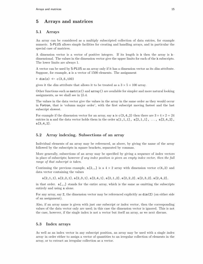
5.1 Arrays

An array can be considered as a multiply subscripted collection of data entries, for examplenumeric. S-PLUS allows simple facilities for creating and handling arrays, and in particular thespecial case of matrices.

A dimension vector is a vector of positive integers. If its length is k then the array is k–dimensional. The values in the dimension vector give the upper limits for each of the k subscripts.The lower limits are always 1.

A vector can be used by S-PLUS as an array only if it has a dimension vector as its dim attribute.Suppose, for example, z is a vector of 1500 elements. The assignment

> dim(z) <- c(3,5,100)

gives it the dim attribute that allows it to be treated as a 3 × 5 × 100 array.

Other functions such as matrix() and array() are available for simpler and more natural lookingassignments, as we shall see in §5.4.

The values in the data vector give the values in the array in the same order as they would occurin Fortran, that is ‘column major order’, with the first subscript moving fastest and the lastsubscript slowest.

For example if the dimension vector for an array, say a is c(3,4,2) then there are 3× 4× 2 = 24entries in a and the data vector holds them in the order a[1,1,1], a[2,1,1], . . . , a[2,4,2],

a[3,4,2].

5.2 Array indexing. Subsections of an array

Individual elements of an array may be referenced, as above, by giving the name of the arrayfollowed by the subscripts in square brackets, separated by commas.

More generally, subsections of an array may be specified by giving a sequence of index vectors

in place of subscripts; however if any index position is given an empty index vector, then the full

range of that subscript is taken.

Continuing the previous example, a[2,,] is a 4 × 2 array with dimension vector c(4,2) anddata vector containing the values

a[2,1,1], a[2,2,1], a[2,3,1], a[2,4,1], a[2,1,2], a[2,2,2], a[2,3,2], a[2,4,2],

in that order. a[,,] stands for the entire array, which is the same as omitting the subscriptsentirely and using a alone.

For any array, say Z, the dimension vector may be referenced explicitly as dim(Z) (on either sideof an assignment).

Also, if an array name is given with just one subscript or index vector, then the correspondingvalues of the data vector only are used; in this case the dimension vector is ignored. This is notthe case, however, if the single index is not a vector but itself an array, as we next discuss.

5.3 Index arrays

As well as an index vector in any subscript position, an array may be used with a single index

array in order either to assign a vector of quantities to an irregular collection of elements in thearray, or to extract an irregular collection as a vector.


A matrix example makes the process clear. In the case of a doubly indexed array, an indexmatrix may be given consisting of two columns and as many rows as desired. The entries in theindex matrix are the row and column indices for the doubly indexed array. Suppose for examplewe have a 4 × 5 array X and we wish to do the following:

• Extract elements X[1,3], X[2,2] and X[3,1] as a vector structure, and

• Replace these entries in the array X by 0s.

In this case we need a 3× 2 subscript array, as in the example given in Figure 1.

> x <- array(1:20,dim=c(4,5)) # Generate a 4 x 5 array.

> x

[,1] [,2] [,3] [,4] [,5]

[1,] 1 5 9 13 17

[2,] 2 6 10 14 18

[3,] 3 7 11 15 19

[4,] 4 8 12 16 20

> i <- array(c(1:3,3:1),dim=c(3,2))

> i # i is a 3 x 2 index array.

[,1] [,2]

[1,] 1 3

[2,] 2 2

[3,] 3 1

> x[i] # Extract those elements

[1] 9 6 3

> x[i] <- 0 # Replace those elements by zeros.

> x

[,1] [,2] [,3] [,4] [,5]

[1,] 1 5 0 13 17

[2,] 2 0 10 14 18

[3,] 0 7 11 15 19

[4,] 4 8 12 16 20

>

Figure 1: Using an index array

As a less trivial example, suppose we wish to generate an (unreduced) design matrix for a blockdesign defined by factors blocks (b levels) and varieties, (v levels). Further suppose there aren plots in the experiment. We could proceed as follows:

> Xb <- matrix(0, n, b)

> Xv <- matrix(0, n, v)

> ib <- cbind(1:n, blocks)

> iv <- cbind(1:n, varieties)

> Xb[ib] <- 1

> Xv[iv] <- 1

> X <- cbind(Xb, Xv)

Further, to construct the incidence matrix, N say, we could use

> N <- crossprod(Xb, Xv)

However a simpler direct way of producing this matrix is to use table():

> N <- table(blocks, varieties)

5.4 The array() function 17

5.4 The array() function

As well as giving a vector structure a dim attribute, arrays can be constructed from vectors bythe array function, which has the form

> Z <- array(data vector,dim vector)

For example, if the vector h contains 24, or fewer, numbers then the command

> Z <- array(h, dim=c(3,4,2))

would use h to set up 3 × 4× 2 array in Z. If the size of h is exactly 24 the result is the same as

> dim(Z) <- c(3,4,2)

However if h is shorter than 24, its values recycled from the beginning again to make it up tosize 24. See §5.4.1 below. As an extreme but common example

> Z <- array(0, c(3,4,2)

makes Z an array of all zeros.

At this point dim(Z) stands for the dimension vector c(3,4,2), and Z[1:24] stands for the datavector as it was in h, and Z[] with an empty subscript or Z with no subscript stands for theentire array as an array.

Arrays may be used in arithmetic expressions and the result is an array formed by element byelement operations on the data vector. The dim attributes of operands generally need to be thesame, and this becomes the dimension vector of the result. So if A, B and C are all similar arrays,then

> D <- 2*A*B + C + 1

makes D a similar array with data vector the result of the evident element by element operations.However the precise rule concerning mixed array and vector calculations has to be considered alittle more carefully.

5.4.1 Mixed vector and array arithmetic. The recycling rule

The precise rule affecting element by element mixed calculations with vectors and arrays issomewhat quirky and hard to find in the references. From experience I have found the followingto be a reliable guide.

• The expression is scanned from left to right.

• Any short vector operands are extended by recycling their values until they match the sizeof any previous (or subsequent) operands.

• As long as short vectors and arrays, only, are encountered, the arrays must all have thesame dim attribute or an error results.

• Any vector operand longer than some previous array immediately converts the calculationto one in which all operands are coerced to vectors. A diagnostic message is issued if thesize of the long vector is not a multiple of the (common) size of all previous arrays.

• If array structures are present and no error or coercion to vector has been precipitated, theresult is an array structure with the common dim attribute of its array operands.

5.5 The outer product of two arrays

An important operation on arrays is the outer product. If a and b are two numeric arrays, theirouter product is an array whose dimension vector is got by concatenating their two dimension


vectors, (order is important), and whose data vector is got by forming all possible products ofelements of the data vector of a with those of b. The outer product is formed by the specialoperator %o%:

> ab <- a %o% b

An alternative is

> ab <- outer(a, b, ’*’)

The multiplication function can be replaced by an arbitrary function of two variables. Forexample if we wished to evaluate the function

f(x, y) =cos(y)

1 + x2

over a regular grid of values with x− and y−coordinates defined by the S-PLUS vectors x and y

respectively, we could proceed as follows:

> f <- function(x,y) cos(y)/(1 + x^2)

> z <- outer(x, y, f)

In particular the outer product of two ordinary vectors is a doubly subscripted array (that is amatrix, of rank at most 1). Notice that the outer product operator is of course non-commutative.Defining your own S-PLUS functions will be considered further in Chapter 9.

5.5.1 An example: Determinants of 2 × 2 digit matrices

As an artificial but cute example, consider the determinants of 2 × 2 matrices

[

a bc d

]

where

each entry is a non-negative integer in the range 0, 1, . . . , 9, that is a digit.

The problem is to find the determinants, ad−bc, of all possible matrices of this form and representthe frequency with which each value occurs as a high density plot. This amounts to finding theprobability distribution of the determinant if each digit is chosen independently and uniformlyat random.

A neat way of doing this uses the outer() function twice:

> d <- outer(0:9, 0:9)

> fr <- table(outer(d, d, "-"))

> plot(as.numeric(names(fr)), fr, type="h",

xlab="Determinant", ylab="Frequency")

Notice the coercion of the names attribute of the frequency table to numeric in order to recoverthe range of the determinant values. The “obvious” way of doing this problem with for–loops,to be discussed in §8.2, is so inefficient as to be impractical.

It is also perhaps surprising that about 1 in 20 such matrices is singular.

5.6 Generalized transpose of an array

The function aperm(a, perm) may be used to permute an array, a. The argument perm mustbe a permutation of the integers {1, 2, . . . , k}, where k is the number of subscripts in a. Theresult of the function is an array of the same size as a but with old dimension given by perm[j]

becoming the new jth dimension. The easiest way to think of this operation is as a generalizationof transposition for matrices. Indeed if A is a matrix, (that is, a doubly subscripted array) thenB given by

> B <- aperm(A, c(2,1))

5.7 Matrix facilities. Multiplication, inversion and solving linear equations. 19

is just the transpose of A. For this special case a simpler function t() is available, so we couldhave used B <- t(A).

5.7 Matrix facilities. Multiplication, inversion and solving linear equa-

tions.

As noted above, a matrix is just an array with two subscripts. However it is such an importantspecial case it needs a separate discussion. S-PLUS contains many operators and functions thatare available only for matrices. For example t(X) is the matrix transpose function, as notedabove. The functions nrow(A) and ncol(A) give the number of rows and columns in the matrixA respectively.

The operator %*% is used for matrix multiplication. An n × 1 or 1 × n matrix may of course beused as an n−vector if in the context such is appropriate. Conversely vectors which occur inmatrix multiplication expressions are automatically promoted either to row or column vectors,whichever is multiplicatively coherent, if possible, (although this is not always unambiguouslypossible, as we see later).

If, for example, A and B are square matrices of the same size, then

> A * B

is the matrix of element by element products and

> A %*% B

is the matrix product. If x is a vector, then

> x %*% A %*% x

is a quadratic form.7

The function crossprod() forms “crossproducts”, meaning that

> crossprod(X, y) is the same as t(X) %*% y

but the operation is more efficient. If the second argument to crossprod() is omitted it is takento be the same as the first.

Other important matrix functions include solve(A, b) for solving equations, solve(A) for thematrix inverse, svd() for the singular value decomposition, qr() for QR decomposition andeigen() for eigenvalues and eigenvectors of symmetric matrices.

The meaning of diag() depends on its argument. diag(vector) gives a diagonal matrix withelements of the vector as the diagonal entries. On the other hand diag(matrix) gives the vectorof main diagonal entries of matrix. This is the same convention as that used for diag() inMATLAB. Also, somewhat confusingly, if k is a single numeric value then diag(k) is the k × kidentity matrix!

A surprising omission from the suite of matrix facilities is a function for the determinant of asquare matrix, however the absolute value of the determinant is easy to calculate for example asthe product of the singular values. (See later.)

5.8 Forming partitioned matrices. cbind() and rbind().

As we have already seen informally, matrices can be built up from other vectors and matricesby the functions cbind() and rbind(). Roughly cbind() forms matrices by binding together

7Note that x %*% x is ambiguous, as it could mean either x′x or xx′, where x is the column form. In suchcases the smaller matrix seems implicitly to be the interpretation adopted, so the scalar x′x is in this case theresult. The matrix xx′ may be calculated either by cbind(x) %*% x or x %*% rbind(x) since the result of rbind()or cbind() is always a matrix.


matrices horizontally, or column-wise, and rbind() vertically, or row-wise.

In the assignment

> X <- cbind(arg1, arg2, arg3, . . . )

the arguments to cbind() must be either vectors of any length, or matrices with the same columnsize, that is the same number of rows. The result is a matrix with the concatenated argumentsarg1, arg2, . . . forming the columns.

If some of the arguments to cbind() are vectors they may be shorter than the column size ofany matrices present, in which case they are cyclically extended to match the matrix column size(or the length of the longest vector if no matrices are given).

The function rbind() does the corresponding operation for rows. In this case any vector argu-ment, possibly cyclically extended, are of course taken as row vectors.

Suppose X1 and X2 have the same number of rows. To combine these by columns into a matrixX, together with an initial column of 1s we can use

> X <- cbind(1, X1, X2)

The result of rbind() or cbind() always has matrix status. Hence cbind(x) and rbind(x)

are possibly the simplest ways explicitly to allow the vector x to be treated as a column or rowmatrix respectively.

5.9 The concatenation function, c(), with arrays.

It should be noted that whereas cbind() and rbind() are concatenation functions that respectdim attributes, the basic c() function does not, but rather clears numeric objects of all dim anddimnames attributes. This is occasionally useful in its own right.

The official way to coerce an array back to a simple vector object is to use as.vector()

> vec <- as.vector(X)

However a similar result can be achieved by using c() with just one argument, simply for thisside-effect:

> vec <- c(X)

There are slight differences between the two, but ultimately the choice between them is largelya matter of style (with the former being preferable).

5.10 Frequency tables from factors. The table() function

Recall that a factor defines a partition into groups. Similarly a pair of factors defines a two waycross classification, and so on. The function table() allows frequency tables to be calculatedfrom equal length factors. If there are k category arguments, the result is a k−way array offrequencies.

Suppose, for example, that statef is a factor giving the state code for each entry in a datavector. The assignment

> statefr <- table(statef)

gives in statefr a table of frequencies of each state in the sample. The frequencies are orderedand labelled by the levels attribute of the category. This simple case is equivalent to, but moreconvenient than,

> statefr <- tapply(statef, statef, length)

5.10 Frequency tables from factors. The table() function 21

Further suppose that incomef is a category giving a suitably defined “income class” for eachentry in the data vector, for example with the cut() function:

> factor(cut(incomes,breaks=35+10*(0:7))) -> incomef

Then to calculate a two-way table of frequencies:

> table(incomef,statef)


35+ thru 45 1 1 0 1 0 0 1 0

45+ thru 55 1 1 1 1 2 0 1 3

55+ thru 65 0 3 1 3 2 2 2 1

65+ thru 75 0 1 0 0 0 0 1 0

Extension to higher way frequency tables is immediate.

22 Lists, data frames, and their uses


6.1 Lists

An S-PLUS list is an object consisting of an ordered collection of objects known as its components.

There is no particular need for the components to be of the same mode or type, and, for example,a list could consist of a numeric vector, a logical value, a matrix, a complex vector, a characterarray, a function, and so on. Here is a simple example of how to make a list:

> Lst <- list(name="Fred", wife="Mary", no.children=3, child.ages=c(4,7,9))

Components are always numbered and may always be referred to as such. Thus if Lst is the nameof a list with four components, these may be individually referred to as Lst[[1]], Lst[[2]],Lst[[3]] and Lst[[4]]. If, further, Lst[[4]] is a vector subscripted array then Lst[[4]][1]

is its first entry.

If Lst is a list, then the function length(Lst) gives the number of (top level) components it has.

Components of lists may also be named, and in this case the component may be referred toeither by giving the component name as a character string in place of the number in doublesquare brackets, or, more conveniently, by giving an expression of the form

> name$component name

for the same thing.

This is a very useful convention as it makes it easier to get the right component if you forget thenumber.

So in the simple example given above:

Lst$name is the same as Lst[[1]] and is the string "Fred",

Lst$wife is the same as Lst[[2]] and is the string "Mary",

Lst$child.ages[1] is the same as Lst[[4]][1] and is the number 4.

It is very important to distinguish Lst[[1]] from Lst[1]. “[[. . .]]” is the operator used toselect a single element, whereas “[. . .]” is a general subscripting operator. Thus the former isthe first object in the list Lst, and if it is a named list the name is not included. The latteris a sublist of the list Lst consisting of the first entry only. If it is a named list, the name is

transferred to the sublist.

The names of components may be abbreviated down to the minimum number of letters neededto identify them uniquely. Thus Lst$coefficients may be minimally specified as Lst$coe andLst$covariance as Lst$cov.

The vector of names is in fact simply an attribute of the list like any other and may be handledas such. Other structures besides lists may, of course, similarly be given a names attribute also.

6.2 Constructing and modifying lists

New lists may be formed from existing objects by the function list(). An assignment of theform

> Lst <- list(name1=object1, name2=object2, . . . ,namem=objectm)

sets up a list Lst of m components using object1, . . . , objectm for the components and givingthem names as specified by the argument names, (which can be freely chosen). If these names areomitted, the components are numbered only. The components used to form the list are copied

when forming the new list and the originals are not affected.

6.3 Some functions returning a list result 23

Lists, like any subscripted object, can be extended by specifying additional components. Forexample

> Lst[5] <- list(matrix=Mat)

6.2.1 Concatenating lists

When the concatenation function c() is given list arguments, the result is an object of mode listalso, whose components are those of the argument lists joined together in sequence.

> list.ABC <- c(list.A, list.B, list.C)

Recall that with vector objects as arguments the concatenation function similarly joined to-gether all arguments into a single vector structure. In this case all other attributes, such as dimattributes, are discarded.

6.3 Some functions returning a list result

Functions and expressions in S-PLUS must return a single object as their result; in cases wherethe result has several component parts, the usual form is that of a list with named components.

6.3.1 Eigenvalues and eigenvectors

The function eigen(Sm) calculates the eigenvalues and eigenvectors of a symmetric matrix Sm.The result of this function is a list of two components named values and vectors. The assign-ment

> ev <- eigen(Sm)

will assign this list to ev. Then ev$val is the vector of eigenvalues of Sm and ev$vec is thematrix of corresponding eigenvectors. Had we only needed the eigenvalues we could have usedthe assignment:

> evals <- eigen(Sm)$values

evals now holds the vector of eigenvalues and the second component is discarded. If the expres-sion

> eigen(Sm)

is used by itself as a command the two components are printed, with their names, at the terminal.

6.3.2 Singular value decomposition and determinants

The function svd(M) takes an arbitrary matrix argument, M, and calculates the singular valuedecomposition of M. This consists of a matrix of orthonormal columns U with the same columnspace as M, a second matrix of orthonormal columns V whose column space is the row space ofM and a diagonal matrix of positive entries D such that M = U %*% D %*% t(V). D is actuallyreturned as a vector of the diagonal elements. The result of svd(M) is actually a list of threecomponents named d, u and v, with evident meanings.

If M is in fact square, then, it is not hard to see that

> absdetM <- prod(svd(M)$d)

calculates the absolute value of the determinant of M. If this calculation were needed often witha variety of matrices it could be defined as an S-PLUS function

> absdet <- function(M) prod(svd(M)$d)


after which we could use absdet() as just another S-PLUS function. As a further trivial butpotentially useful example, you might like to consider writing a function, say tr(), to calculatethe trace of a square matrix. [Hint: You will not need to use an explicit loop. Look again at thediag() function.]

Functions will be discussed formally later in these notes.

6.3.3 Least squares fitting and the QR decomposition

The function lsfit() returns a list giving results of a least squares fitting procedure. Anassignment such as

> ans <- lsfit(X, y)

gives the results of a least squares fit where y is the vector of observations and X is the designmatrix. See the help facility for more details, and also for the follow-up function ls.diag()

for, among other things, regression diagnostics. Note that a grand mean term is automaticallyincluded and need not be included explicitly as a column of X.

Another closely related function is qr() and its allies. Consider the following assignments

> Xplus <- qr(X)

> b <- qr.coef(Xplus, y)

> fit <- qr.fitted(Xplus, y)

> res <- qr.resid(Xplus, y)

These compute the orthogonal projection of y onto the range of X in fit, the projection ontothe orthogonal complement in res and the coefficient vector for the projection in b, that is, b isessentially the result of the MATLAB ‘backslash’ operator.

It is not assumed that X has full column rank. Redundancies will be discovered and removed asthey are found.

This alternative is the older, low level way to perform least squares calculations. Although stilluseful in some contexts, it would now generally be replaced by the statistical models features, aswill be discussed in §10.

6.4 Data frames

A data frame is a list with class data.frame. There are restrictions on lists that may be madeinto data frames, namely

• The components must be vectors (numeric, character, or logical), factors, numeric matrices,lists, or other data frames.

• Matrices, lists, and data frames provide as many variables to the new data frame as theyhave columns, elements, or variables, respectively.

• Numeric vectors and factors are included as is, and non-numeric vectors are coerced to befactors, whose levels are the unique values appearing in the vector.

• Vector structures appearing as variables of the data frame must all have the same length,and matrix structures must all have the same row size.

Data frames may in many ways be regarded as a matrix with columns possibly of differing modesand attributes. It may be displayed in matrix form, and its rows and columns extracted usingmatrix indexing conventions.

6.4 Data frames 25

6.4.1 Making data frames

Objects satisfying the restrictions placed on the columns (components) of a data frame may beused to form one using the function data.frame:

> accountants <- data.frame(home=statef,loot=income, shot=incomef)

A list whose components conform to the restrictions of a data frame may be coerced into a dataframe using the function as.data.frame()

The simplest way to construct a data frame from scratch is to use the read.table() function toread an entire data frame from an external file. This is discussed further in §7.

6.4.2 attach() and detach()

The $ notation, such as accountants$statef, for list components is not always very convenient.A useful facility would be somehow to make the components of a list or data frame temporarilyvisible as variables under their component name, without the need to quote the list name explicitlyeach time.

The attach() function, as well as having a directory name as its argument, may also have adata frame. Thus suppose lentils is a data frame with three variables lentils$u, lentils$v,lentils$w. The attach

> attach(lentils)

places the data frame in the search list at position 2, and provided there are no variables u, v orw in position 1, u, v and w are available as variables from the data frame in their own right. Atthis point an assignment such as

> u <- v+w

does not replace the component u of the data frame, but rather masks it with another variableu in the working directory at position 1 on the search list. To make a permanent change to thedata frame itself, the simplest way is to resort once again to the $ notation:

> lentils$u <- v+w

However the new value of component u is not visible until the data frame is detached and attachedagain.

To detach a data frame, use the function

> detach()

More precisely, this statement detaches from the search list the entity currently at position 2.Thus in the present context the variables u, v and w would be no longer visible, except under thelist notation as lentils$u and so on.

NOTE: With the current release of S-PLUS the search list can contain at most 20 items. Avoidattaching the same data frame more than once. Always detach the data frame as soon as youhave finished using its variables.

6.4.3 Working with data frames

A useful convention that allows you to work with many different problems comfortably togetherin the same working directory is

• gather together all variables for any well defined and separate problem in a data frameunder a suitably informative name;


• when working with a problem attach the appropriate data frame at position 2, and use theworking directory at level 1 for operational quantities and temporary variables;

• before leaving a problem, add any variables you wish to keep for future reference to thedata frame using the $ form of assignment, and then detach();

• finally remove all unwanted variables from the working directory and keep it as clean ofleft-over temporary variables as possible.

In this way it is quite simple to work with many problems in the same directory, all of whichhave variables named x, y and z, for example.

6.4.4 Attaching arbitrary lists

attach() is a generic function that allows not only directories and data frames to be attachedto the search list, but other classes of object as well. In particular any object of mode list maybe attached in the same way:

> attach(any.old.list)

It is also possible to attach objects of class pframe, to so-called parametrized data frames, neededfor nonlinear regression and elsewhere.

Being a generic function it is also possible to add methods for attaching yet more classes of objectshould the need arise.

Reading data from files 27

7 Reading data from files

Large data objects will usually be read as values from external files rather than entered duringan S-PLUS session at the keyboard. S-PLUS input facilities are simple and their requirements arefairly strict and even rather inflexible. There is a clear presumption by the designers of S-PLUS

that you will be able to modify your input files using other tools, such file editors and the UNIX

utilities sed and awk to fit in with the requirements of S-PLUS. Generally this is very simple.

There is, however, a function make.fields() that can be used to convert a file with fixedwidth, non separated, input fields into a file with separated fields. There is also a facilitycount.fields() that will count the number of fields on each line of such a file. Occasion-ally for very simple conversion and checking problems these may be adequate to the task, but inmost cases it is better to do the preliminary spade work before the S-PLUS session begins.

If variables are to be held mainly in data frames, as we strongly suggest, they should be, anentire data frame can be read directly with the read.table() function. There is also an older,more primitive input function, scan(), that is still occasionally useful in special circumstances.

7.1 The read.table() function

To read an entire data frame directly, the external file will normally have a special form.

• The first line of the file should have a name for each variable in the data frame.

• Each additional line of the file has its first item a row label and the values for each variable.

If the file has one fewer item in its first line than in its second, this arrangement is presumed tobe in force. So the first few lines of a file to be read as a data frame might look as in Figure 2.By default numeric items (except row labels) are read as numeric variables and non-numeric

Price Floor Area Rooms Age Cent.heat

01 52.00 111.0 830 5 6.2 no

02 54.75 128.0 710 5 7.5 no

03 57.50 101.0 1000 5 4.2 no

04 57.50 131.0 690 6 8.8 no

05 59.75 93.0 900 5 1.9 yes

...

Figure 2: Input file form with names and row labels

variables, such as Cent.heat in the example, as factors. This can be changed if necessary.

The function read.table() can then be used to read the data frame directly

> HousePrice <- read.table("houses.data")

Often you will want to omit including the row labels directly and use the default labels. In thiscase the file may omit the row label column as in Figure 3. The data frame may then be read as

> HousePrice <- read.table("houses.data", header=T)

where the heading=T option specifies that the first line is a line of headings, and hence, byimplication from the form of the file, that no explicit row labels are given.

7.2 The scan() function

Suppose the data vectors are of equal length and are to be read in in parallel. Further supposethat there are three vectors, the first of mode character and the remaining two of mode numeric,

28 Reading data from files

Price Floor Area Rooms Age Cent.heat

52.00 111.0 830 5 6.2 no

54.75 128.0 710 5 7.5 no

57.50 101.0 1000 5 4.2 no

57.50 131.0 690 6 8.8 no

59.75 93.0 900 5 1.9 yes

...

Figure 3: Input file form without row labels

and the file is input.dat. The first step is to use scan() to read in the three vectors as a list,as follows

> in <- scan("input.dat", list("",0,0))

The second argument is a dummy list structure that establishes the mode of the three vectorsto be read. The result, held in in, is a list whose components are the three vectors read in. Toseparate the data items into three separate vectors, use assignments like

> label <- in[[1]]; x <- in[[2]]; y <- in[[3]]

More conveniently, the dummy list can have named components, in which case the names can beused to access the vectors read in. For example

> in <- scan("input.dat", list(id="", x=0, y=0))

If you wish to access the variables separately they may either be re-assigned to variables in theworking frame:

> label <- in$id; x <- in$x; y <- in$y

or the list may be attached at position 2 of the search list, (see §6.4.4).

If the second argument is a single value and not a list, a single vector is read in, all componentsof which must be of the same mode as the dummy value.

> X <- matrix(scan("light.dat", 0), ncol=5, byrow=T)

There are more elaborate input facilities available and these are detailed in the manual.

7.3 Other facilities; editing data

Once a data set has been read, there is an X–window based facility in S-PLUS for making smallchanges. The command

> xnew <- data.ed(xold)

will allow you to edit your data set xold using a spreadsheet-like environment in a separateediting window, and on completion the changed object is assigned to xnew. xold, and hencexnew, can be any matrix, vector, data frame, or atomic data object.

More language features. Loops and conditional execution 29

8 More language features. Loops and conditional execu-

tion

8.1 Grouped expressions

S-PLUS is an expression language in the sense that its only command type is a function orexpression which returns a result. Even an assignment is an expression whose result is thevalue assigned, and it may be used wherever any expression may be used; in particular multipleassignments are possible.

Commands may be grouped together in braces, {expr1; expr2;. . . ; exprm}, in which case thevalue of the group is the result of the last expression in the group evaluated. Since such a groupis also an expression it may, for example, be itself included in parentheses and used a part of aneven larger expression, and so on.

8.2 Control statements

8.2.1 Conditional execution: if statements

The language has available a conditional construction of the form

> if (expr1) expr2 else expr3

where expr1 must evaluate to a logical value and the result of the entire expression is then evident.

8.2.2 Repetitive execution: for loops, repeat and while

There is also a for–loop construction which has the form

> for (name in expr1) expr2

where name is the loop variable. expr1 is a vector expression, (often a sequence like 1:20),and expr2 is often a grouped expression with its sub-expressions written in terms of the dummyname. expr2 is repeatedly evaluated as name ranges through the values in the vector result ofexpr1.

As an example, suppose ind is a vector of class indicators and we wish to produce separate plotsof y versus x within classes. One possibility here is to use coplot() to be discussed later, whichwill produce an array of plots corresponding to each level of the factor. Another way to do this,now putting all plots on the one display, is as follows:

> yc <- split(y, ind); xc <- split(x, ind)

> for (i in 1:length(yc)){plot(xc[[i]], yc[[i]]);

abline(lsfit(xc[[i]], yc[[i]]))}

(Note the function split() which produces a list of vectors got by splitting a larger vector ac-cording to the classes specified by a category. This is a useful function, mostly used in connectionwith boxplots. See the help facility for further details.)

WARNING: for() loops are very slow in the present version of S-PLUS and should be avoidedif possible. Many functions, such as apply(), tapply(), sapply() and others, are writtenprimarily to avoid using explicit for() loops.

Other looping facilities include the

> repeat expr

statement and the

30 More language features. Loops and conditional execution

> while (condition) expr

statement.

The break statement can be used to terminate any loop, possibly abnormally. For repeat loops,this is the only way to terminate them.

The next can be used to discontinue one particular cycle and skip to the “next”.

Control statements are most often used in connection with functions which are discussed in §9,and where more examples will emerge.

Writing your own functions 31

9 Writing your own functions

As we have seen informally along the way, the S-PLUS language allows the user to create objectsof mode function. These are true S-PLUS functions that are stored in a special internal form andmay be used in further expressions and so on. In the process the language gains enormously inpower, convenience and elegance, and learning to write useful functions is one of the main waysto make your use of S-PLUS comfortable and productive.

It should be emphasized that most of the functions supplied as part of the S-PLUS system, suchas mean(), var(), postscript() and so on, are themselves written in S-PLUS and thus do notdiffer materially from user written functions.

A function is defined by an assignment of the form

> name <- function(arg1, arg2, . . . ) expression

The expression is an S-PLUS expression, (usually a grouped expression), that uses the arguments,argi, to calculate a value. The value of the expression is the value returned for the function.

A call to the function then usually takes the form name(expr1, expr2, . . . ) and may occuranywhere a function call is legitimate.

9.1 Simple examples

As a first example, consider a function to calculate the two sample t−statistic, showing “all thesteps”. This is an artificial example, of course, since there are other, simpler ways of achievingthe same end.

The function is defined as follows:

> twosam <- function(y1, y2) {

n1 <- length(y1); n2 <- length(y2)

yb1 <- mean(y1); yb2 <- mean(y2)

s1 <- var(y1); s2 <- var(y2)

s <- ((n1-1)*s1 + (n2-1)*s2)/(n1+n2-2)

tst <- (yb1 - yb2)/sqrt(s2*(1/n1 + 1/n2))

tst

}

With this function defined, you could perform two sample t−tests using a call such as

> tstat <- twosam(datamale, datafemale); tstat

As a second example, consider a function to emulate directly the MATLAB backslash command,which returns the coefficients of the orthogonal projection of the vector y onto the column space ofthe matrix, X . (This is ordinarily called the least squares estimates of the regression coefficients).This would ordinarily be done with the qr() function; however this is sometimes a bit tricky touse directly and it pays to have a simple function such as the following to use it safely.

Thus given a vector yn×1 and a matrix Xn×p then

X\y =def. (X ′X)−X ′y

where (X ′X)− is a generalised inverse of X ′X .

> bslash <- function(X, y) {

X <- qr(X)

qr.coef(X, y)

}


After this object is created it is permanent, like all objects, and may be used in statements suchas

> regcoeff <- bslash(Xmat, yvar)

and so on.

The classical S-PLUS function lsfit() does this job quite well, and more. It in turn uses thefunctions qr() and qr.coef() in the slightly counterintuitive way above to do this part of thecalculation. Hence there is probably some value in having just this part isolated in a simple touse function if it is going to be in frequent use. If so, we may wish to make it a matrix binaryoperator for even more convenient use.

9.2 Defining new binary operators.

Had we given the bslash() function a different name, namely one of the form

%anything%

it could have been used as a binary operator in expressions rather than in function form. Suppose,for example, we choose ! for the internal character. The function definition would then start as

> "%!%" <- function(X, y) {. . . }

(Note the use of quote marks.) The function could then be used as X %!% y. (The backslashsymbol itself is not a convenient choice as it presents special problems in this context.)

The matrix multiplication operator, %*%, and the outer product matrix operator %o% are otherexamples of binary operators defined in this way.

9.3 Named arguments and defaults. “. . .”

As first noted in §2.3 if arguments to called functions are given in the “name=object” form, theymay be given in any order. Furthermore the argument sequence may begin in the unnamed,positional form, and specify named arguments after the positional arguments.

Thus if there is a function fun1 defined by

> fun1 <- function(data, data.frame, graph, limit) {. . . 8}

Then the function may be invoked in several ways, for example

> ans <- fun1(d, df, 20, T)

> ans <- fun1(d, df, graph=T, limit=20)

> ans <- fun1(data=d, limit=20, graph=T, data.frame=df)

are all equivalent.

In many cases arguments can be given commonly appropriate default values, in which case theymay be omitted altogether from the call when the defaults are appropriate. For example, if fun1were defined as

> fun1 <- function(data, data.frame, graph=T, limit=20) {. . . 8}

it could be called as

> ans <- fun1(d, df)

which is now equivalent to the three cases above, or as

8This ellipsis is used as a customary typographical device to mean an abridgment. This is not the case in thelatter part of this section.

9.4 Assignments within functions are local. Frames. 33

> ans <- fun1(d, df, limit=10)

which changes one of the defaults.

It is important to note that defaults may be arbitrary expressions, even involving other argumentsto the same function; they are not restricted to be constants as in our simple example here.

Another frequent requirement is to allow one function to pass on argument settings to another.For example many graphics functions use the function par() and functions like plot() allow theuser to pass on graphical parameters to par() to control the graphical output. (See §11.4.1 formore details on the par() function.) This can be done by including an extra argument, literally“. . . ”, of the function, which may then be passed on. An outline example is given in Figure 4.

fun1 <- function(data, data.frame, graph=T, limit=20, ...) {

[omitted statements]

if (graph)

par(pch="*", ...)

[more omissions]

}

Figure 4: Use of the ellipsis argument, “. . . ”

Note here that the ellipses, “. . . ” are literal S-PLUS, not a typographical device.

9.4 Assignments within functions are local. Frames.

Note that any ordinary assignments done within the function are local and temporary and are

lost after exit from the function. Thus the assignment X <- qr(X) does not affect the value ofthe argument in the calling program.

To understand completely the rules governing the scope of S-PLUS assignments the reader needsto be familiar with the notion of an evaluation frame. This is a somewhat advanced, thoughhardly difficult, topic and is not covered further in these notes.

If global and permanent assignments are intended within a function, then the ‘superassignment’operator, ‘<<-’ can be used. See the help document for details, and also see the synchronize()

function.

9.5 More advanced examples

9.5.1 Efficiency factors in block designs

As a more complete, if a little pedestrian, example of a function, consider finding the efficiencyfactors for a block design. (Some aspects of this problem have already been discussed in §5.3.)

A block design is defined by two factors, say blocks (b levels) and varieties, (v levels). If Rv×v

and Kb×b are the replications and block size matrices, and N b×v is the incidence matrix, thenthe efficiency factors are defined as the eigenvalues of the matrix

E = Iv − R−1/2N ′K−1NR−1/2 = Iv − A′A

where A = K−1/2NR−1/2. One way to write the function is as in Figure 5.


> bdeff <- function(blocks, varieties) {

blocks <- as.factor(blocks) # minor safety move

b <- length(levels(blocks))

varieties <- as.factor(varieties) # minor safety move

v <- length(levels(varieties))

K <- as.vector(table(blocks)) # remove dim attr

R <- as.vector(table(varieties)) # remove dim attr

N <- table(blocks, varieties)

A <- 1/sqrt(K) * N * rep(1/sqrt(R), rep(b, v))

sv <- svd(A)

list(eff=1 - sv$d^2, blockcv=sv$u, varietycv=sv$v)

}

Figure 5: A function for block design efficiencies

It is numerically slightly better to work with the singular value decomposition on this occasionrather than the eigenvalue routines.

The result of the function is a list giving not only the efficiency factors as the first component,but also the block and variety canonical contrasts, since sometimes these give additional usefulqualitative information.

9.5.2 Dropping all names in a printed array

For printing purposes with large matrices or arrays, it is often useful to print them in close blockform without the array names or numbers. Removing the dimnames attribute will not achievethis effect, but rather the array must be given a dimnames attribute consisting of empty strings.For example to print a matrix, X

> temp <- X

> dimnames(temp) <- list(rep("", nrow(X)), rep("", ncol(X))

> temp; rm(temp)

This can be much more conveniently done using a function, no.dimnames(), shown in Figure 6,as a “wrap around” to achieve the same result. It also illustrates how some effective and usefuluser functions can be quite short. With this function defined, an array may be printed in close

no.dimnames <- function(a){

#

# Remove all dimension names from an array for compact printing.

#

d <- list()

l <- 0

for(i in dim(a)) {

d[[l <- l + 1]] <- rep("", i)

}

dimnames(a) <- d

a

}

Figure 6: A function for printing arrays in compact form

format using

9.6 Customising the environment. .First and .Last 35

> no.dimnames(X)

This is particularly useful for large integer arrays, where patterns are the real interest ratherthan the values.

9.5.3 Recursive numerical integration

Functions may be recursive, and may themselves define functions within themselves. Note,however, that such functions, or indeed variables, are not inherited by called functions in higherevaluation frames as they would be if they were on the search list.

The example in Figure 7 shows a naive way of performing one dimensional numerical integration.The integrand is evaluated at the end points of the range and in the middle. If the one-paneltrapezium rule answer is close enough to the two panel, then the latter is returned as the value.Otherwise the same process is recursively applied to each panel. The result is an adaptive inte-gration process that concentrates function evaluations in regions where the integrand is farthestfrom linear. There is, however, a heavy overhead, and the function is only competitive with otheralgorithms when the integrand is both smooth and very difficult to evaluate.

The example is also given partly as a little puzzle in S-PLUS programming.

area <- function(f, a, b, eps = 1.0e-06, lim = 10)

{

fun1 <- function(f, a, b, fa, fb, a0, eps, lim, fun)

{

d <- (a + b)/2

h <- (b - a)/4

fd <- f(d)

a1 <- h * (fa + fd)

a2 <- h * (fd + fb)

if(abs(a0 - a1 - a2) < eps || lim == 0)

return(a1 + a2)

else {

return(fun(f, a, d, fa, fd, a1, eps, lim - 1, fun) +

fun(f, d, b, fd, fb, a2, eps, lim - 1, fun))

}

}

fa <- f(a)

fb <- f(b)

a0 <- ((fa + fb) * (b - a))/2

fun1(f, a, b, fa, fb, a0, eps, lim, fun1)

}

Figure 7: A recursive function within a function

9.6 Customising the environment. .First and .Last

Any function named .First() in the .Data directory has a special status. It is automaticallyperformed at the beginning of an S-PLUS session and may be used to initialise the environment.For example, the definition in Figure 8 alters the prompt to $ and sets up various other usefulthings that can then be taken for granted in the rest of the session. Similarly a function .Last(),if defined, is executed at the very end of the session. An example is given in Figure 9.


> .First <- function() {

options(prompt="$ ", continue="+\t") # $ is the prompt

options(digits=5, length=999) # custom numbers and printout

options(gui="motif") # default graphics user interface

tek4014() # for terminal work

par(pch = "+") # plotting character

attach(paste(unix("echo $HOME"), "/.Data", sep = ""))

# Home of my personal library

library(examples) # attach also the system examples

}

Figure 8: An example of a .First() function

> .Last <- function() {

graphics.off() # a small safety measure.

cat(paste(unix("date"),"\nAdios\n")) # Is it time for lunch?

}

Figure 9: An example of a .Last() function

9.7 Classes, generic functions and object orientation

The class of an object determines how it will be treated by what are known as generic functions.Put the other way round, a generic function performs a task or action on its arguments specific

to the class of the argument itself. If the argument lacks any class attribute, or has a classnot catered for specifically by the generic function in question, there is always a default action

provided.

An example makes things clearer. In a sense the print() function has always been generic, sinceits action is to adopt a style of output appropriate to its arguments. Thus a matrix appears as amatrix, a vector as a vector, and so on. (Note that the print() function can be called explicitly,or implicitly by giving an expression as a complete command.)

The August 1991 release of S-PLUS increases the number of such functions, alters the mechanismby which they are implemented and via the class mechanism offers the user the facility of designingand writing generic functions for special purposes. Among the other new, or newly genericfunctions are plot() for displaying objects graphically, summary() for summarising analyses ofvarious types, and anova() for comparing statistical models.

The number of generic functions that can treat a class in a specific way can be quite large.For example, the functions that can accommodate in some fashion objects of class data.frame

include[, [[<-, dbdetach, dimnames<-, pairs, signif,

[<-, aperm, dim, formula, plot, summary,

[[, atan, dimnames, ordered<-, print, t,

A currently complete list can be got by using the methods() function:

> methods(class="data.frame")

Conversely the number of classes a generic function can handle can also be quite large. Forexample the plot() function has variants for classes of object

data.frame, default, glm, pregam, surv.fit,

design, factor, lm, preloess, tree,

formula, gam, loess, profile, tree.sequence,

9.7 Classes, generic functions and object orientation 37

and perhaps more. A complete list can be got again by using the methods() function:

> methods(plot)

The reader is referred to the official references for a complete discussion of this mechanism.

38 Statistical models in S-PLUS


This section presumes the reader has some familiarity with statistical methodology, in particularwith regression analysis and the analysis of variance. Later we make some rather more ambitiouspresumptions, namely that something is known about generalized linear models and nonlinearregression.

The requirements for fitting statistical models are sufficiently well defined to make it possibleto construct general tools that apply in a broad spectrum of problems. Since the August 1991release S-PLUS provides an interlocking suite of facilities that make fitting statistical models verysimple. However these are not at the same high level as those in, say, Genstat, especially in theform of the output which in keeping with general S-PLUS policy is rather minimal.

10.1 Defining statistical models; formulæ

The template for a statistical model is a linear regression model with independent, homoscedasticerrors

yi =

p∑

j=0

βjxij + ei, ei ∼ NID(0, σ2), i = 1, 2, . . . , n

In matrix terms this would be written

y = Xβ + e

where the y is the response vector, X is the model matrix or design matrix and has columnsx0, x1, . . ., xp, the determining variables. Very often x0 will be a column of 1s defining anintercept term.

Examples.

Before giving a formal specification, a few examples may usefully set the picture.

Suppose y, x, x0, x1, x2, . . . are numeric variables, X is a matrix and A, B, C, . . . are factors. Thefollowing formulæ on the left side below specify statistical models as described on the right.

y ~ x

y ~ 1 + x

Both imply the same simple linear regression model of y on x. The first has animplicit intercept term, and the second an explicit one.

y ~ -1 + x

y ~ x - 1

Simple linear regression of y on x through the origin, (that is, without an inter-cept term).

log(y) ~ x1 + x2 Multiple regression of the transformed variable, log(y), on x1 and x2 (with animplicit intercept term).

y ~ poly(x,2)

y ~ 1 + x + I(x^2)

Polynomial regression of y on x of degree 2. The first form uses orthogonalpolynomials, and the second uses explicit powers, as basis.

y ~ X + poly(x,2) Multiple regression y with model matrix consisting of the matrix X as well aspolynomial terms in x to degree 2.

y ~ A Single classification analysis of variance model of y, with classes determined byA.

y ~ A + x Single classification analysis of covariance model of y, with classes determinedby A, and with covariate x.

10.1 Defining statistical models; formulæ 39

y ~ A*B

y ~ A + B + A:B

y ~ B %in% A

y ~ A/B

Two factor non-additive model of y on A and B. The first two specify the samecrossed classification and the second two specify the same nested classification.In abstract terms all four specify the same model subspace.

y ~ (A + B + C)^2

y ~ A*B*C - A:B:C

Three factor experiment but with a model containing main effects and two factorinteractions only. Both formulæ specify the same model.

y ~ A * x

y ~ A/x

y ~ A/(1 + x) - 1

Separate simple linear regression models of y on x within the levels of A, withdifferent codings. The last form produces explicit estimates of as many differentintercepts and slopes as there are levels in A.

y ~ A*B + Error(C) An experiment with two treatment factors, A and B, and error strata determinedby factor C. For example a split plot experiment, with whole plots, (and hencealso subplots), determined by factor C.

The operator ~ is used to define a model formula in S-PLUS. The form, for an ordinary linearmodel, is

response ~ [±] term1 ± term2 ± term3 ± · · ·

response is a vector or matrix, (or expression evaluating to a vector or matrix) defining theresponse variable(s).

± is an operator, either + or -, implying the inclusion or exclusion of a term in the model, (thefirst is optional).

term is either

• a vector or matrix expression, or 1,

• a factor, or

• a formula expression consisting of factors, vectors or matrices connected by formula

operators.

In all cases each term defines a collection of columns either to be added to or removed fromthe model matrix. A 1 stands for an intercept column and is by default included in themodel matrix unless explicitly removed.

The formula operators are similar in effect to the Wilkinson and Rogers notation used by suchprograms a Glim and Genstat. One inevitable change is that the operator “.” becomes “:” sincethe period is a valid name character in S-PLUS. The notation is summarised as in the Table 1(based on Chambers & Hastie, p. 29).

Note that inside the parentheses that usually enclose function arguments all operators have theirnormal arithmetic meaning. The function I() is an identity function used only to allow termsin model formulæ to be defined using arithmetic operators.

Note particularly that the model formulæ specify the columns of the model matrix, specification ofthe parameters is implicit. This is not the case in other contexts, for example in fitting nonlinearmodels


Form Meaning

Y ~ M Y is modelled as M

M1 + M2 Include M1 and M2

M1 - M2 Include M1 leaving out terms of M2

M1:M2 The tensor product of M1 and M2. If both terms factors, then the“subclasses” factor.

M1 %in% M2 Similar to M1:M2, but with a different coding.

M1*M2 M1 + M2 + M1:M2

M1/M2 M1 + M2 %in% M1

M^n All terms in M together with “interactions” up to order n

I(M) Insulate M . Inside M all operators have their normal arithmeticmeaning, and that term appears in the model matrix.

Table 1: Summary of model operator semantics

10.2 Regression models; fitted model objects

The basic function for fitting ordinary multiple models is lm(), and a streamlined version of thecall is as follows:

> fitted.model <- lm(formula, data=data.frame)

For example

> fm2 <- lm(y ~ x1 + x2, data=production)

would fit a multiple regression model of y on x1 and x2 (with implicit intercept term).

The important but technically optional parameter data=production specifies that any variablesneeded to construct the model should come first from the production data frame. This is the

case regardless of whether data frame production has been attached to the search list or not.

10.3 Generic functions for extracting information

The value of lm() is fitted model object; technically a list of results of class lm. Informationabout the fitted model can then be displayed, extracted, plotted and so on by using genericfunctions that orient themselves to objects of class lm. A full list of these at the present time is

add1 coef effects kappa predict residuals

alias deviance family labels print summary

anova drop1 formula plot proj

A brief description of the most commonly used ones is given in Table 2.

10.4 Analysis of variance; comparing models

The model fitting function aov(formula, data=data.frame) operates at the simplest level in avery similar way to the function lm(), and most of the generic functions listed in Table 2 apply.

10.4 Analysis of variance; comparing models 41

Function Value or Effect

anova(object1,

object2)

Compare a submodel with an outer model and productan analysis of variance table.

coefficients(object) Extract the regression coefficient (matrix).Short form: coef(object).

deviance(object) Residual sum of squares, weighted if appropriate.

formula(object) Extract the model formula.

plot(object) Product two plots, one of the observations against thefitted values, the other of the absolute residuals againstthe fitted values.

predict(object,

newdata=data.frame)

predict.gam(object,

newdata=data.frame)

The data frame supplied must have variables specifiedwith the same labels as the original. The value is a vec-tor or matrix of predicted values corresponding to thedetermining variable values in data.frame.predict.gam() is a safe alternative to predict() thatcan be used for lm, glm and gam fitted objects. It mustbe used, for example, in cases where orthogonal polyno-mials are used as the original basis functions, and theaddition of new data implies different basis functions tothe original.

print(object) Print a concise version of the object.Most often used implicitly.

residuals(object) Extract the (matrix of) residuals, weighted as appropri-ate. Short form: resid(object).

summary(object) Print a comprehensive summary of the results of the re-gression analysis.

Table 2: Commonly used generic functions on class lm objects

It should be noted that in addition aov() allows an analysis of models with multiple error stratasuch as split plot experiments, or balanced incomplete block designs with recovery of inter-blockinformation. The model formula

response ~ mean.formula + Error(strata.formula)

specifies a multi-stratum experiment with error strata defined by the strata.formula. In thesimplest case, strata.formula is simply a factor, when it defines a two strata experiment, namelybetween and within the levels of the factor.

For example, with all determining variables factors, a model formula such as that in:

> fm <- aov(yield ~ v + n*p*k + Error(farms/blocks), data=farm.data)

would typically be used to describe an experiment with mean model v + n*p*k and three errorstrata, namely “between farms”, “within farms, between blocks” and “within blocks”.

10.4.1 ANOVA tables

Note also that the analysis of variance table (or tables) are for a sequence of fitted models. Thesums of squares shown are the decrease in the residual sums of squares resulting from an inclusion


of that term in the model at that place in the sequence. Hence only for orthogonal experimentswill the order of inclusion be inconsequential.

For multistratum experiments the procedure is first to project the response onto the error strata,again in sequence, and to fit the mean model to each projection. For further details, see Chambersand Hastie, §5.

A more flexible alternative to the default full ANOVA table is to compare two or more modelsdirectly using the anova() function.

> anova(fitted.model.1, fitted.model.2, . . . )

The display is then an ANOVA table showing the differences between the fitted models whenfitted in sequence. The fitted models being compared would usually be an hierarchical sequence,of course. This does not give different information to the default, but rather makes it easier tocomprehend and control.

10.5 Updating fitted models. The ditto name “.”

The update() function is largely a convenience function that allows a model to be fitted thatdiffers from one previously fitted usually by just a few additional or removed terms. Its form is

> new.model <- update(old.model, new.formula)

In the new.formula the special name consisting of a period, “.”, only, can be used to stand for“the corresponding part of the old model formula”. For example

> fm05 <- lm(y ~ x1 + x2 + x3 + x4 + x5, data=production)

> fm6 <- update(fm05, . ~ . + x6)

> smf6 <- update(fm6, sqrt(.) ~ .)

would fit a five variate multiple regression with variables (presumably) from the data frameproduction, fit an additional model including a sixth regressor variable, and fit a variant on themodel where the response had a square root transform applied.

Note especially that if the data= argument is specified on the original call to the model fittingfunction, this information is passed on through the fitted model object to update() and its allies.

The name “.” can also be used in other contexts, but with slightly different meaning. Forexample

> fmfull <- lm(y ~ . , data=production)

would fit a model with response y and regressor variables all other variables in the data frame

production.

Other functions for exploring incremental sequences of models are add1(), drop1(), step() andstepwise(). The names of these give a good clue to their purpose, but for full details see thehelp document.

10.6 Generalized linear models; families

Generalized linear modelling is a development of linear models to accommodate both non-normalresponse distributions and transformations to linearity in a clean and straightforward way. Ageneralized linear model may be described in terms of the following sequence of assumptions:

• There is a response, y, of interest and stimulus variables x1, x2, . . . whose values influencethe distribution of the response.

10.6 Generalized linear models; families 43

• The stimulus variables influence the distribution of y through a single linear function, only.This linear function is called the linear predictor, and is usually written

η = β1x1 + β2x2 + · · · + βpxp

hence xi has no influence on the distribution of y if and only if βi = 0.

• The distribution of y is of the form

fY (y; µ, ϕ) = exp

[

A

ϕ{yλ(µ) − γ (λ(µ))} + τ(y, ϕ)

]

where ϕ is a scale parameter, (possibly known), and is constant for all observations, Arepresents a prior weight, assumed known but possibly varying with the observations, andµ is the mean of y. So it is assumed that the distribution of y is determined by its meanand possibly a scale parameter as well.

• The mean, µ, is a smooth invertible function of the linear predictor:

µ = m(η), η = m−1(µ) = `(µ)

and this inverse function, `(.) is called the link function.

These assumptions are loose enough to encompass a wide class of models useful in statisticalpractice, but tight enough to allow the development of a unified methodology of estimation andinference, at least approximately. The reader is referred to any of the current reference works onthe subject for full details, such as

Generalized linear models by Peter McCullagh and John A Nelder, 2nd edition, Chapmanand Hall, 1989, or

An introduction to generalized linear models by Annette J Dobson, Chapman and Hall,1990.

10.6.1 Families

The class of generalized linear models handled by facilities supplied in S-PLUS includes gaussian,binomial, poisson, inverse gaussian and gamma response distributions and also quasi-likelihood

models where the response distribution is not explicitly specified. In the latter case the variance

function must be specified as a function of the mean, but in other cases this function is impliedby the response distribution.

Each response distribution admits a variety of link functions to connect the mean with the linearpredictor. Those automatically available are as in Table 3.

The combination of a response distribution, a link function and various other pieces of informationthat are needed to carry out the modelling exercise is called the family of the generalized linearmodel.

10.6.2 The glm() function

Since the distribution of the response depends on the stimulus variables through a single linearfunction only, the same mechanism as was used for linear models can still be used to specify thelinear part of a generalized model. The family has to be specified in a different way.

The S-PLUS function to fit a generalized linear model is glm() which uses the form

> fitted.model <- glm(formula, family =family.generator, data=data.frame)

The only new feature is the family.generator, which is the instrument by which the family isdescribed. It is the name of a function that generates a list of functions and expressions that


Family Name

Link Function binomial gaussian Gamma inverse.gaussian poisson quasi

logit ? ?

probit ? ?

cloglog ? ?

identity ? ? ? ?

inverse ? ?

log ? ? ?

1/mu^2 ? ?

sqrt ? ?

Table 3: Families and the link functions available to them

together define and control the model and estimation process. Although this may seem a littlecomplicated at first sight, its use is quite simple.

The names of the standard, supplied family generators are given under “Family Name” in Table 3.Where there is a choice of links, the name of the link may also be supplied with the family name,in parentheses as a parameter. In the case of the quasi family, the variance function may alsobe specified in this way.

Some examples make the process clear.

The gaussian family

A call such as

> fm <- glm(y ~ x1+x2, family=gaussian, data=sales)

achieves the same result as

> fm <- lm(y ~ x1+x2, data=sales)

but much less efficiently. Note how the gaussian family is not automatically provided with achoice of links, so no parameter is allowed. If a problem requires a gaussian family with anonstandard link, this can usually be achieved through the quasi family, as we shall see later.

The binomial family

Consider a small, artificial example.

On the Greek island of Kalythos the male inhabitants suffer from a congenital eye disease, theeffects of which become more marked with increasing age. Samples of islander males of variousages were tested for blindness and the results recorded. The data is shown in Table 4.

The problem we consider is to fit both logistic and probit models to this data, and to estimatefor each model the LD50, that is the age at which the chance of blindness for a male inhabitantis 50%.

If y is the number of blind at age x and n the number tested, both models have the form

y ∼ B(n, F (β0 + β1x))

10.6 Generalized linear models; families 45

Age: 20 35 45 55 70

No. tested: 50 50 50 50 50

No. blind: 6 17 26 37 44

Table 4: The Kalythos blindness data

where for the probit case, F (z) = Φ(z) is the standard normal distribution function, and in thelogit case, (the default), F (z) = ez/(1 + ez). In both cases the LD50 is

LD50 = −β0/β1

that is, the point at which the argument of the distribution function is zero.

The first step is to set the data up as a data frame

> kalythos <- data.frame(x=c(20,35,45,55,70), n=rep(50,5),

y=c(6,17,26,37,44))

To fit a binomial model using glm() there are two possibilities for the response:

• If the response is a vector it is assumed to hold binary data, and so must be a 0, 1 vector.

• If the response is a two column matrix it is assumed that the first column holds the numberof successes for the trial and the second holds the number of failures.

Here we need the second of these conventions, so we add a matrix to our data frame:

> kalythos$Ymat <- cbind(kalythos$y, kalythos$n - kalythos$y)

To fit the models we use

> fmp <- glm( Ymat~x, family=binomial(link=probit), data=kalythos)

> fml <- glm( Ymat~x, family=binomial, data=kalythos)

Since the logit link is the default the parameter may be omitted on the second call. To see theresults of each fit we could use

> summary(fmp)

> summary(fml)

Both models fit (all too) well. To find the LD50 estimate we can use a simple function:

> ld50 <- function(b) -b[1]/b[2]

> ldp <- ld50(coef(fmp)); ldl <- ld50(coef(fmp)); c(ldp, ldl)

The actual estimates from this data are 43.663 years and 43.601 years respectively.

Poisson models

With the poisson family the default link is the log, and in practice the major use of this familyis to fit surrogate poisson log-linear models to frequency data, whose actual distribution is oftenmultinomial. This is a large and important subject we will not discuss further here. It evenforms a major part of the use of non-gaussian generalized models overall.

Occasionally genuinely poisson data arises in practice and in the past it was often analysed asgaussian data after either a log or a square-root transformation. As a graceful alternative to thelatter, a poisson generalized linear model may be fitted as in the following example:

> fmod <- glm(y ~ A+B + x, family=poisson(link=sqrt), data=worm.counts)


Quasi-likelihood models

For all families the variance of the response will depend on the mean and will have the scaleparameter as a multiplier. The form of dependence of the variance on the mean is a characteristicof the response distribution; for example for the poisson distribution Var[y] = µ.

For quasi-likelihood estimation and inference the precise response distribution is not specified,but rather only a link function and the form of the variance function as it depends on the mean.Since quasi-likelihood estimation uses formally identical techniques to those for the gaussian dis-tribution, this family provides a way of fitting gaussian models with non-standard link functionsor variance functions, incidently.

For example, consider fitting the non-linear regression

y =θ1z1

z2 − θ2

+ e (1)

this may be written alternatively as

y =1

β1x1 + β2x2

+ e

where x1 = z2/z1, x2 = −1/x1, β1 = 1/θ1 and β2 = θ2/θ1. Supposing a suitable data frame tobe set up we could fit this non-linear regression as

> nlfit <- glm(y~x1+x2-1,family=

quasi(link=inverse,variance=constant), data=biochem)

The reader is referred to the manual and the help document for further information, as needed.

10.7 Nonlinear regression models; parametrized data frames

S-PLUS provides two functions to fit nonlinear models that do not conform even to the partiallylinear paradigm of generalized linear models. These are ms() for arbitrary minimization problemswhere the objective functions is a sum of similar terms, and nls() for conventional nonlinearleast squares estimation of normal nonlinear regression models.

In this brief introduction we only consider the nonlinear regression function nls() and leave ms()for the reader to pursue as needed.

10.7.1 Changes to the form of the model formula

In specifying a linear, or generalized linear model we could allow the regression parameters to bedefined implicitly, and to be given names by transference from the column of the model matrixthat they multiply.

In arbitrary nonlinear models no such simplicity applies and we have to specify the model asan ordinary expression that includes both determining variables and parameters together. Forexample to specify a model for a nonlinear regression such as 1 above, we would use

y ~ t1*x1/(x2 - t2)

where y is the response variable, x1 and x2 are determining variables and t1 and t2 are scalarparameters.

In such model formulæ all operators have their usual arithmetic expression meaning, and theuseful facility of expanding factors and forming cross and nested structures is no longer available.All parameters must be explicitly defined in the formula, even if they come from a linear part ofthe model.

10.8 Some non-standard models 47

10.7.2 Specifying the parameters

Since the model formula now contains both determining variables and parameters, there has tobe some mechanism for specifying which are which. But of course once the parameters have beenspecified the remaining variates in the model formula must be variables.

As well as specifying which are the parameters, it is also necessary in this case to specify aninitial approximation for each with which to start the iterative estimation procedure.

There are two ways of specifying this information:

• If the call to nls() has a start= parameter specified, its value must be a list of namedcomponents. The names of the list specify the names of the parameters and the valuesspecify the starting values.

• If the data is held in a data frame, the parameters may similarly be defined as a parameters

attribute of the data frame.

Since our policy is generally to work with data frames as much as follows, we show the secondpossibility in the next example.

Example

Consider again a nonlinear regression of the form 1. An easy way to find initial estimates for theparameters is to regress x2y on x1 and x2:

> fm0 <- lm(x2*y ~ x1 + x2 - 1, data=biochem)

> th <- coef(fm0)

To name the parameters and associate them with the biochem is done as follows:

> parameters(biochem) <- list(t1=th[1], t2=th[2])

Now to fit the nonlinear regression model:

> fm <- nls(y ~ t1*x1/(x2 - t2), data=biochem)

At this point we could use the summary() function and most of the other generics to investigatethe model and display information. To extract the coefficients we could now use, for example

> th <- coef(fm)

and to make these least squares estimates the new values of the parameters associated withbiochem we could simply repeat the step

> parameters(biochem) <- list(t1=th[1], t2=th[2])

Note that the function parameters() may either be used as an expression, in which case it ex-tracts the list of parameters from a data frame, or it may be used as the target for an assignment,in which case it accepts a parameter list for a specified data frame. In this respect it is verysimilar to the attributes() function. There is also a function param() analogous to attr(),which handles one parameter at a time under a character string name.

10.8 Some non-standard models

We conclude this section with just a brief mention of some of the other facilities available inS-PLUS for special regression and data analysis problems.

Local approximating regressions. The loess() function fits a nonparametric regression byusing a locally weighted regression. Such regressions are useful for highlighting a trend inmessy data or for data reduction to give some insight into a large data set.


Robust regression There are several functions available for fitting regression models in a wayresistant to the influence of extreme outliers in the data. The most sophisticated of theseis rreg(), but others include lmsfit() for least median squares regression and l1fit()

for regression using the L1−norm. However these do not as yet have the facility of usingformulæ to specify the model function, for example, and conform to an older protocol, whichmakes them sometimes rather tedious to use. There is also a robust() facility to changea glm family object into a robust version for use with the glm() model fitting function.

Generalized additive models. This technique aims to construct a regression function fromsmooth additive functions of the determining variables, usually one for each determiningvariable. The function gam() is in many ways similar to the other model fitting functionsoutlined above. In addition there are other model fitting functions that do a similar job.These include avas() and ace(). On the other hand ppreg() is available for projectionpursuit regression, but this technique is still very much in need of a complete theoreticaltreatment and further practical experience. These latter functions are again conformingto an older protocol for model fitting functions and lack the convenience of the newerfunctions.

Tree based models Rather than seek an explicit global linear model for prediction or inter-pretation, tree based models seek to bifurcate the data, recursively, at critical points ofthe determining variables in order to partition the data ultimately into groups that are ashomogeneous as possible within, and as heterogeneous as possible between. The resultsoften lead to insights that other data analysis methods tend not to yield.

Models are again specified in the ordinary linear model form. The model fitting functionis tree(), but many other generic functions such as plot() and text() are well adaptedto displaying the results of a tree-based model fit in a graphical way.

Graphical procedures 49

11 Graphical procedures

The graphical facilities are an important and extremely versatile component of the S-PLUS envi-ronment. Best results are obtained when S-PLUS is used with a high quality graphics system suchas X−windows, although even a simple ASCII terminal can be quite effective for some purposes.

Before the graphical facilities of S-PLUS may be used, it is necessary to inform S-PLUS what typeof device is being used by starting a device driver. In an X−windows environment, the commandto do this may be

> X11()

(which creates a separate window in which high-quality graphical output will appear,) or for asimpler graphics terminal the command

> tek4014()

may be appropriate.

Once a device driver is running S-PLUS plotting commands can be used to construct and displaygraphical objects. Plotting commands are divided into three basic groups:

High-level plotting functions create a new plot on the graphics device, possibly with axes,labels, titles and so on.

Low-level plotting functions add more information to an existing plot, such as extra points,lines and labels.

Interactive graphics functions allow you interactively add information to, or extract informationfrom, an existing plot, using a pointing device such as a mouse.

Furthermore, S-PLUS maintains a list of graphical parameters which allow you to customise yourplots.

11.1 High-level plotting commands

High-level plotting functions are designed to generate a complete plot of the data passed asarguments to the function. Where appropriate, axes, labels and titles are automatically generated(unless you request otherwise.) High-level plotting commands always start a new plot, erasingthe current plot if necessary.

11.1.1 The plot() function

One of the most frequently used plotting functions in S-PLUS is the plot() function. This isa generic function: the type of plot produced is dependent on the type or class of the firstargument.

plot(x,y)

plot(xy)

If x and y are vectors, plot(x,y) produces a scatterplot of x against y.The same effect can be produced by supplying one argument (second form)as either a list containing two elements x and y or a two-column matrix.

plot(x) Produces a time series plot if x is a numeric vector or time series object,or an Argand diagram if x is a complex vector.

plot(f)

plot(f,y)

f is a factor object, y is a numeric vector. The first form generates a barplot of f; the second form produces boxplots of y for each level of f.


plot(df)

plot(~ expr)

plot(y ~ expr)

df is a data frame, y is any object, expr is a list of object names separatedby ‘+’ (e.g. a + b + c). The first two forms produce distributional plotsof the variables in a data frame (first form) or of a number of namedobjects (second form). The third form plots y against every object namedin expr.

11.1.2 Displaying multivariate data

S-PLUS provides two very useful functions for representing multivariate data. If X is a numericmatrix or data frame, the command

> pairs(X)

produces a pairwise scatterplot matrix of the variables defined by the columns of X, that is,every column of X is plotted against every other column of X and the resulting n(n− 1) plots arearranged in a matrix with plot scales constant over the rows and columns of the matrix.

When three or four variables are involved a coplot may be more enlightening. If a and b arenumeric vectors and c is a numeric vector or factor object (all of the same length), then thecommand

> coplot(a ~ b | c)

produces a number of scatterplots of a against b for given values of c. If c is a factor, this simplymeans that a is plotted against b for every level of c. When c is numeric, it is divided intoa number of conditioning intervals and for each interval a is plotted against b for values of cwithin the interval. The number and position of intervals can be controlled with given.values=

argument to coplot() — the function co.intervals() is useful for selecting intervals. You canalso use two given variables with a command like

> coplot(a ~ b | c + d)

which produces scatterplots of a against b for every joint conditioning interval of c and d.

The coplot() and pairs() function both take an argument panel= which can be used to cus-tomise the type of plot which appears in each panel. The default is points() to produce ascatterplot but by supplying some other low-level graphics function of two vectors x and y as thevalue of panel= you can produce any type of plot you wish. An example panel function usefulfor coplots is panel.smooth().

11.1.3 Display graphics

Other high-level graphics functions produce different types of plots. Some examples are:

tsplot(x1,x2,...) Plots any number of time series on the same scale. This automatic simul-taneous scaling feature is also useful when the xi’s are ordinary numericvectors, in which case they are plotted against the numbers 1, 2, 3, . . ..

qqnorm(x)

qqplot(x,y)

Distribution-comparison plots. The first form plots the numeric vectorx against the expected Normal order scores (a normal scores plot.) Thesecond form plots the quantiles of x against those of y to compare theirrespective distributions.

11.1 High-level plotting commands 51

hist(x)

hist(x,nclass=n)

hist(x,

breaks=. . .)

Produces a histogram of the numeric vector x. A sensible number of classesis usually chosen, but a recommendation can be given with the nclass=

argument. Alternatively, the breakpoints can be specified exactly withthe breaks= argument. If the probability=T argument is given, the barsrepresent relative frequencies instead of counts.

dotchart(x,. . .) Construct a dotchart of the data in x. In a dotchart the y−axis gives alabelling of the data in x and the x−axis gives its value. For example itallows easy visual selection of all data entries with values lying in specifiedranges.

pie(slices,

names,

explode=. . .)

Make a pie diagram, including the possibility of some pieces displacedor exploded out from the centre. (Pie diagrams are especially good forshowing to administrators and bosses, but not much else, in my opinion.)

11.1.4 Arguments to high-level plotting functions

There are a number of arguments which may be passed to high-level graphics functions, as follows:

add=T Forces the function to act as a low-level graphics function, superimposingthe plot on the current plot (some functions only).

axes=F Suppresses generation of axes — useful for adding your own custom axeswith the axis() function. The default, axes=T, means include axes.

log="x"

log="y"

log="xy"

Causes the x, y or both axes to be logarithmic. Only works for scatterplots(and variants).

type= The type= argument controls the type of plot produced, as follows:

type="p" Plot individual points (the default)

type="l" Plot lines

type="b" Plot points connected by lines (both)

type="o" Plot points overlaid by lines

type="h" Plot vertical lines from points to the zero axis (high-density)

type="s"

type="S"

Step-function plots. In the first form, the top of the vertical defines thepoint; in the second, the bottom.

type="n" No plotting at all. However axes are still drawn (by default) and thecoordinate system is set up according to the data. Ideal for creating plotswith subsequent low-level graphics functions.

xlab="string"

ylab="string"

Axis labels for the x and y axes. Use these arguments to change the defaultlabels, usually the names of the objects used in the call to the high-levelplotting function.

main="string" Figure title, placed at the top of the plot in a large font.

sub="string" Sub-title, placed just below the x-axis in a smaller font.


11.2 Low-level plotting commands

Sometimes the high-level plotting functions don’t produce exactly the kind of plot you desire.In this case, low-level plotting commands can be used to add extra information (such as points,lines or text) to the current plot.

Some of the more useful low-level plotting functions are:

points(x,y)

lines(x,y)

Adds points or connected lines to the current plot. plot()’s type= ar-gument can also be passed to these functions (and defaults to "p" forpoints() and "l" for lines().)

text(x, y,

labels, . . . )

Add text to a plot at points given by x, y. Normally labels is an integeror character vector in which case labels[i] is plotted at point (x[i],

y[i]). The default is 1:length(x).

Note: This function is often used in the sequence> plot(x, y, type="n"); text(x, y, names)

The graphics parameter type="n" suppresses the points but sets up theaxes, and the text() function supplies special characters, as specified bythe character vector names for the points.

abline(a, b)

abline(h=y)

abline(v=x)

abline(lm.obj)

Adds a line of slope b and intercept a to the current plot. h=y may be usedto specify y-coordinates for the heights of horizontal lines to go across aplot, and v=x similarly for the x-coordinates for vertical lines. Also lm.obj

may be list with a $coefficients component of length 2 (such as theresult of model-fitting functions,) which are taken as an intercept andslope, in that order.

polygon(x, y,

. . . )

Draws a polygon defined by the ordered vertices in (x,y). and (optionally)shade it in with hatch lines, or fill it if the graphics device allows the fillingof figures.

legend(x,y,

legend,...)

Adds a legend to the current plot at the specified position. Plotting charac-ters, line styles, colours etc. are ¡identified with the labels in the charactervector legend. At least one other argument v (a vector the same lengthas legend) with the corresponding values of the plotting unit must alsobe given, as follows:

legend( ,angle=v) Shading angles

legend( ,

density=v)

Shading densities

legend( ,fill=v) Colours for filled boxes

legend( ,col=v) Colours in which points or lines will be drawn

legend( ,lty=v) Line styles

legend( ,pch=v) Plotting characters (character vector)

legend( ,marks=v) Plotting symbols, as obtained when using a numeric argument to pch=

(numeric vector).

11.3 Interactive graphics functions 53

title(main,sub) Adds a title main to the top of the current plot in a large font and (op-tionally) a sub-title sub at the bottom in a smaller font.

axis(side,...) Adds an axis to the current plot on the side given by the first argument(1 to 4, counting clockwise from the bottom.) Other arguments controlthe positioning of the axis within or beside the plot, and tick positionsand labels. Useful for adding custom axes after calling plot() with theaxes=F argument.

Low-level plotting functions usually require some positioning information (e.g. x and y coordi-nates) to determine where to place the new plot elements. Coordinates are given in terms ofuser coordinates which are defined by the previous high-level graphics command and are chosenbased on the supplied data.

Where x and y arguments are required, it is also sufficient to supply a single argument beinga list with elements named x and y. Similarly a matrix with two columns is also valid input.In this way functions such as locator() (see below) may be used to specify positions on a plotinteractively.

11.3 Interactive graphics functions

S-PLUS also provides functions which allow users to extract or add information to a plot usinga mouse. The simplest of these is the locator() function:

locator(n,type) Waits for the user to select locations on the current plot using the leftmouse button. This continues until n (default 500) points have been se-lected, or the middle mouse button is pressed. The type argument allowsfor plotting at the selected points and has the same effect as for high-levelgraphics commands; the default is no plotting. locator() returns thelocations of the points selected as a list with two components x and y.

locator() is usually called with no arguments. It is particularly useful for interactively selectingpositions for graphic elements such as legends or labels when it is difficult to calculate in advancewhere the graphic should be placed. For example, to place some informative text near an outlyingpoint, the command

> text(locator(1), "Outlier", adj=0)

may be useful. locator() will still work if the current device does not support a mouse; in thiscase the user will be prompted for x and y coordinates.

identify(x,y,

labels)

Allow the user to highlight any of the points defined by x and y (using theleft mouse button) by plotting the corresponding component of labelsnearby (or the index number of the point if labels is absent). Returnsthe indices of the selected points when the middle button is pressed.


Sometimes we want to identify particular points on a plot, rather than their positions. Forexample, we may wish the user to select some observation of interest from a graphical displayand then manipulate that observation in some way. Given a number of (x, y) coordinates in twonumeric vectors x and y, we could use the identify() function as follows:

> plot(x,y)

> identify(x,y)

The identify() functions performs no plotting itself, but simply allows the user to move themouse pointer and click the left mouse button near a point. The point nearest the mouse pointerwill be highlighted with its index number (that is, its position in the x/y vectors) plotted nearby.Alternatively, you could use some informative string (such as a case name) as a highlight byusing the labels argument to identify(), or disable highlighting altogether with the plot=F

argument. When the middle button is pressed, identify() returns the indices of the selectedpoints; you can use these indices to extract the selected points from the original vectors x and y.

11.4 Using graphics parameters

When creating graphics, particularly for presentation or publication purposes, S-PLUS does notalways produce exactly that which is required. You can, however, customise almost every aspectof the display using graphics parameters. S-PLUS maintains a list of a large number of graphicsparameters which control things such as line style, colours, figure arrangement and text justifi-cation among many others. Every graphics parameter has a name (such as ‘col’, which controlscolours,) and a value (a colour number, for example.)

A separate list of graphics parameters is maintained for each active device, and each device hasa default set of parameters when initialised. Graphics parameters can be set in two ways: eitherpermanently, affecting all graphics functions which access the current device; or temporarily,affecting only a single graphics function call.

11.4.1 Permanent changes: The par() function

The par() function is used to access and modify the list of graphics parameters for the currentgraphics device.

par() Without arguments, returns a list of all graphics parameters and theirvalues for the current device.

par(c("col",

"lty"))

With a character vector argument, returns only the named graphics pa-rameters (again, as a list.)

par(col=4,lty=2) With named arguments (or a single list argument) , sets the values ofthe named graphics parameters, and returns the original values of theparameters as a list.

Setting graphics parameters with the par() function changes the value of the parameters per-

manently, in the sense that all future calls to graphics functions (on the current device) willbe affected by the new value. You can think of setting graphics parameters in this way as set-ting ‘default’ values for the parameters, which will be used by all graphics functions unless analternative value is given.

11.5 Graphics parameters list 55

Note that calls to par() always affect the global values of graphics parameters, even when par()

is called from within a function. This is often undesirable behaviour — usually we want to setsome graphics parameters, do some plotting, and then restore the original values so as not toaffect the user’s S-PLUS session. You can restore the initial values by saving the result of par()when making changes, and restoring the initial values when plotting is complete.

> oldpar <- par(col=4,lty=2)

. . . plotting commands . . .

> par(oldpar)

11.4.2 Temporary changes: Arguments to graphics functions

Graphics parameters may also be passed to (almost) any graphics function as named arguments.This has the same effect as passing the arguments to the par() function, except that the changesonly last for the duration of the function call. For example:

> plot(x,y,pch="+")

produces a scatterplot using a plus sign as the plotting character, without changing the defaultplotting character for future plots.

11.5 Graphics parameters list

The following sections detail many of the commonly-used graphical parameters. The S-PLUS

help documentation for the par() function provides a more concise summary; this is providedas a somewhat more detailed alternative.

Graphics parameters will be presented in the following form:

name=value A description of the parameter’s effect. name is the name of the parameter,that is, the argument name to use in calls to par() or a graphics function.value is a typical value you might use when setting the parameter.

11.5.1 Graphical elements

S-PLUS plots are made up of points, lines, text and polygons (filled regions.) Graphical param-eters exist which control how these graphical elements are drawn, as follows:

pch="+" Character to be used for plotting points. The default varies with graphicsdrivers, but it is usually ‘*’ for terminals or window devices, and ‘•’ forPostScript devices. Plotted points tend to appear slightly above or belowthe appropriate position unless you use "." as the plotting character,which produces centred points.

pch=4 When pch is given as an integer between 0 and 18 inclusive, a specialisedplotting symbol is produced. To see what the symbols are, use the com-mand

> legend(locator(1),as.character(0:18),marks=0:18)


lty=2 Line types. Alternative line styles are not supported on all graphics devices(and vary on those that do) but line type 1 is always a solid line, and linetypes 2 and onwards are dotted or dashed lines, or some combination ofboth.

lwd=2 Line widths. Desired width of lines, in multiples of the ‘standard’ linewidth. Affects axis lines as well as lines drawn with lines(), etc.

col=2 Colours to be used for points, lines, text, filled regions and images. Eachof these graphic elements has a list of possible colours, and the value ofthis parameter is an index to that list. Obviously, this parameter appliesonly to a limited range of devices.

font=2 Font to use for text. The appropriate value of this parameter is dependenton the graphics device being used; for the postscript() device this is anindex to the system dataset ps.fonts.

adj=-0.1 Justification of text relative to the plotting position. 0 means left justify, 1means right justify and 0.5 means to centre horizontally about the plottingposition. The actual value is the proportion of text that appears to theleft of the plotting position, so a value of -0.1 leaves a gap of 10% of thetext width between the text and the plotting position.

cex=1.5 Character expansion. The value is the desired size of text characters (in-cluding plotting characters) relative to the default text size.

11.5.2 Axes and tick marks

Many of S-PLUS’s high-level plots have axes, and you can construct axes yourself with the low-level axis() graphics function. Axes have three main components: the axis line (line stylecontrolled by the lty graphics parameter), the tick marks (which mark off unit divisions alongthe axis line) and the tick labels (which mark the units.) These components can be customisedwith the following graphics parameters.

lab=c(5,7,12) The first two numbers are the desired number of tick intervals on the xand y axes respectively. The third number is the desired length of axislabels, in characters (including the decimal point.) Choosing a too-smallvalue for this parameter may result in all tick labels being rounded to thesame number!

las=1 Orientation of axis labels. 0 means always parallel to axis, 1 means alwayshorizontal, and 2 mean always perpendicular to the axis.

mgp=c(3,1,0) Positions of axis components. The first component is the distance fromthe axis label to the axis position, in text lines. The second componentis the distance to the tick labels, and the final component is the distancefrom the axis position to the axis line (usually zero). Positive numbersmeasure outside the plot region, negative numbers inside.

11.5 Graphics parameters list 57

tck=0.01 Length of tick marks, as a fraction of the size of the plotting region. Whentck is small (less than 0.5) the tick marks on the x and y axes are forcedto be the same size. A value of 1 gives grid lines. Negative values give tickmarks outside the plotting region. Use tck=0.01 and mgp=c(1,-1.5,0)

for internal tick marks.

xaxs="s"

yaxs="d"

Axis styles for the x and y axes, respectively. With styles "s" (standard)and "e" (extended) the smallest and largest tick marks always lie outsidethe range of the data. Extended axes may be widened slightly if any pointsare very near the edge. This style of axis can sometimes leave large blankgaps near the edges. With styles "i" (internal) and "r" (the default) tickmarks always fall within the range of the data, however style "r" leaves asmall amount of space at the edges.

Setting this parameter to "d" (direct axis) locks in the current axis anduses it for all future plots (or until the parameter is set to one of the othervalues above, at least.) Useful for generating series of fixed-scale plots.

11.5.3 Figure margins

A single plot in S-PLUS is known as a figure and comprises a plot region surrounded by margins(possibly containing axis labels, titles, etc.) and (usually) bounded by the axes themselves. Atypical figure appears in Figure 10. Graphics parameters controlling figure layout include:

6

?

6

� - -

. . . . . . . . . . . . . . . . . . . . . . . . . . . .............................

mai[2]

mar[3]

**

*

*

*

*

*

*

*

*

*

*

*

y

mai[1] x

Plot region

Margin

Figure 10: Anatomy of an S figure


mai=

c(1,0.5,0.5,0)

Widths of the bottom, left, top and right margins, respectively, measuredin inches.

mar=c(4,2,2,1) Similar to mai, except the measurement unit is text lines.

mar and mai are equivalent in the sense that setting one changes the value of the other. Thedefault values chosen for this parameter are often too large; the right-hand margin is rarelyneeded, and neither is the top margin if no title is being used. The bottom and left margins mustbe large enough to accommodate the axis and tick labels. Furthermore, the default is chosenwithout regard to the size of the device surface: for example, using the postscript() driverwith the height=4 argument will result in a plot which is about 50% margin unless mar or maiare set explicitly. When multiple figures are in use (see below) the margins are reduced by half,however this may not be enough when many figures share the same page.

11.5.4 Multiple figure environment

S-PLUS allows you to create an n × m array of figures on a single page. Each figure has itsown margins, and the array of figures is optionally surrounded by an outer margin as shown inFigure 11.

The graphical parameters relating to multiple figures are as follows:

mfcol=c(3,2)

mfrow=c(2,4)

Set size of multiple figure array. The first value is the number of rows;the second is the number of columns. The only difference between thesetwo parameters is that setting mfcol causes figures to be filled by column;mfrow fills by rows. The arrangement in Figure 11 would have been createdby setting mfrow=c(3,2); the figure shows the page after four plots havebeen drawn.

mfg=c(2,2,3,2) Position of current figure in a multiple figure environment. The first twonumbers are the row and column of the current figure; the last two arethe number of rows and columns in the multiple figure array. Set thisparameter to jump between figures in the array. You can even use differentvalues for the last two numbers than the true values for unequally-sizedfigures on the same page.

fig=c(4,9,1,4)/10 Position of the current figure on the page. Values are the positions of theleft, right, bottom and top edges respectively, as a percentage of the pagemeasured from the bottom left corner. The example value would be fora figure in the bottom right of the page. Set this parameter for arbitrarypositioning of figures within a page.

oma=c(2,0,3,0)

omi=c(0,0,0.8,0)

Size of outer margins. Like mar and mai, the first measures in text linesand the second in inches, starting with the bottom margin and workingclockwise.

Outer margins are particularly useful for page-wise titles, etc. Text can be added to the outermargins with the mtext() function with argument outer=T. There are no outer margins bydefault, however, so you must create them explicitly using oma or omi.

11.6 Device drivers 59

� -

6

?

��

HH��QQ�

�

*****

****

*

**

* * **

**

****

*

omi[2] omi[3]mfrow=c(3,2)

oma[1]

mfg=c(2,2,3,2)

Figure 11: Page layout in multiple figure mode

11.6 Device drivers

S-PLUS can generate graphics (of varying levels of quality) on almost any type of display orprinting device. Before this can begin, however, S-PLUS needs to be informed what type ofdevice it is dealing with. This is done by starting a device driver. The purpose of a device driveris to convert graphical instructions from S-PLUS (‘draw a line,’ for example) into a form that theparticular device can understand.

Device drivers are started by calling a device driver function. There is one such function for everydevice driver: type help(Devices) for a list of them all. For example, issuing the command

> postscript()

causes all future graphics output to be sent to the printer in PostScript format. Some commonly-used device drivers are:


motif()

openlook()

X11()

For use with the X11 or Open Windows window systems.

suntools() For use with the SunView windowing system.

postscript() For printing on PostScript printers, or creating PostScript graphics files.

printer()

crt()

For terminals with little or no graphics capabilities. ASCII-based graphicsare generated.

When you have finished with a device, be sure to terminate the device driver by issuing thecommand

> dev.off()

This ensures that the device finishes cleanly; for example in the case of hardcopy devices thisensures that every page is completed and has been sent to the printer.

11.6.1 PostScript diagrams for typeset documents.

By passing the file argument to the postscript() device driver function, you may store thegraphics in PostScript format in a file of your choice. The plot will be in portrait orientationunless the horizontal=T argument is given, and you can control the size of the graphic with thewidth and height arguments (the plot will be scaled as appropriate to fit these dimensions.) Forexample, the command

> postscript("file.ps", height=4)

will produce a file containing PostScript code for a figure four inches high, perhaps for inclusionin a document.9 It is important to note that if the file named in the command already exists, itwill be overwritten. This is the case even if the file was only created earlier in the same S-PLUS

session.

11.6.2 Multiple graphics devices

In advanced use of S-PLUS it is often useful to have several graphics devices in use at the sametime. Of course only one graphics device can accept graphics commands at any one time, andthis is known as the current device. When multiple devices are open, they form a numberedsequence with names giving the kind of device at any position.

The main commands used for operating with multiple devices, and their meanings are as follows:

motif()

postscript()

. . .

Each new call to a device driver function opens a new graphics device,thus extending by one the device list. This device becomes the currentdevice, to which graphics output will be sent.

dev.list() returns the number and name of all active devices. The device at position1 on the list is always the null device which does not accept graphicscommands at all.

9Warning: The PostScript code produced by the postscript() device driver is not Encapsulated PostScript,and thus including it in a document electronically (as opposed to physical cut-and-paste) can be rather problematic.For this type of application, a better solution is to use the fig() driver (available from statlib) and use a conversionprogram, such as fig2dev, to convert the resultant fig code to Encapsulated PostScript.

11.6 Device drivers 61

dev.next()

dev.prev()

returns the number and name of the graphics device next to, or previousto the current device, respectively.

dev.set(which=k) can be used to change the current graphics device to the one at positionk of the device list. Returns the number and label of the device.

dev.off(k) Terminate the graphics device at point k of the device list. For somedevices, such as postscript devices, this will either print the file imme-diately or correctly complete the file for later printing, depending on howthe device was initiated.

dev.copy(device,

. . . , which=k)

dev.print(device,

. . . , which=k)

Make a copy of the device k. Here device is a device function, such aspostscript, with extra arguments, if needed, specified by . . . . dev.printis similar, but the copied device is immediately closed, so that end ac-tions, such as printing hardcopies, are immediately performed. (See alsoprintgraph()).

graphics.off() Terminate all graphics devices on the list, except the null device.

62 S-PLUS: An introductory session

A S-PLUS: An introductory session

The following session is intended to introduce to you some features of the S-PLUS environmentby using them. Many features of the system will be unfamiliar and puzzling at first, but this willsoon disappear.

login:

. . .

> ls -a

> ls -a .Data

Login, start your windowing system (ask a demonstrator if youneed help), and check that your working directory has a subdi-rectory .Data, which in turn contains the files .First, .Lastand possibly .Audit.

You should also have the file morley.data in your working di-rectory. If not, see a demonstrator. If you have, proceed.

> Splus -e Start Splus with the inbuilt command line editor enabled.

The S-PLUS program begins, with a banner.

(Within S-PLUS the prompt on the left hand side will not be shown

to avoid confusion.)

help.start() Start the help facility. You should briefly explore the featuresof this facility with the mouse. Standard X window conventionsapply.

Iconify the help window and move on to the next part.

motif() Turn on the graphics window. You may need to re-position andre-size to make it convenient to work with both windows.

x <- rnorm(50)

y <- rnorm(x)

Generate two pseudo random normal vectors of x− and y−co-ordinates.

hull <- chull(x, y) Find their convex hull in the plane.

plot(x, y)

polygon(x[hull], y[hull],

dens=15)

Plot the points in the plane, and mark in their convex hull.

objects() See which S-PLUS objects are now in the .Data directory.

rm(x,y,hull) Remove objects no longer needed. (Clean up).

x <- 1:20 Make x = (1, 2, . . . , 20)

w <- 1 + sqrt(x)/2 A ‘weight’ vector of standard deviations.

dummy <- data.frame(x=x,

y= x + rnorm(x)*w)

dummy

Make a data frame of two columns, x and y, and look at it.

fm <- lm(y~x, data=dummy)

summary(fm)

Fit a simple linear regression of y on x and look at the analysis.

fm1 <- lm(y~x, data=dummy,

weight=1/w^2)

summary(fm1)

Since we know the standard deviations, we can do a weightedregression.

lrf <- loess(y~x, dummy) Make a nonparametric local regression function.

attach(dummy) Make the columns in the data frame visible as variables.

plot(x, y) Standard point plot.

lines(x, fitted(lrf)) Add in the local regression.

S-PLUS: An introductory session 63

abline(0, 1, lty=3) The true regression line: (intercept 0, slope 1).

abline(coef(fm)) Unweighted regression line.

abline(coef(fm1),lty=4) Weighted regression line.

At any time you can make a hardcopy of the graphics windowby clicking on the Graph section of the window and selectingthe Print option.

detach() Remove data frame from the search list.

plot(fitted(fm),

resid(fm),

xlab="Fitted values",

ylab="Residuals", main=

"Residuals vs Fitted")

A standard regression diagnostic plot to check for heteroscedas-ticity. Can you see it?

qqnorm(resid(fm), main=

"Residuals Rankit Plot")

A normal scores plot to check for skewness, kurtosis and out-liers. (Not very useful here.)

rm(fm,fm1,lrf,x,dummy) Clean up again.

The next section will look at data from the classical experimentof Michaelson and Morley to measure the speed of light.

!more morley.data Optional. Temporarily interrupt S-PLUS and look at the file.This is a standard way to escape to the operating system.

mm <- read.table(

"morley.data")

mm

Read in the Michaelson and Morley data as a data frame, andlook at it. There are five experiments (col. Expt) and each has20 runs (col. Run) and sl is the recorded speed of light, suitablycoded.

attach(mm, 1)

objects()

Place mm on the top of the search list, (position 1).

Expt <- factor(Expt)

Run <- factor(Run)

Change Expt and Run into factors.

detach(1, save="mm")

attach(mm)

Save the changes and make the data frame visible at position 2(the default).

plot(Expt,Speed, main=

"Speed of Light Data",

xlab="Experiment No.")

Compare the five experiments with simple boxplots.

fm <- aov(Speed~Run+Expt,

data=mm)

summary(fm)

Analyse as a randomized block, with ‘runs’ and ‘experiments’as factors.

fm0 <- update(fm,

.~.-Run)

anova(fm0,fm)

Fit the sub-model omitting ‘runs’, and compare using a formalanalysis of variance.

detach()

rm(fm, fm0)

Clean up before moving on.

We now look at some more graphical features: contour and3−dimensional perspective plots.

x <- seq(-pi, pi, len=50)

y <- x

x is a vector of 50 equally spaced values in −π ≤ x ≤ π. y isthe same.

64 S-PLUS: An introductory session

f <- outer(x, y,

function(x,y)

cos(y)/(1+x^2))

f is a square matrix, with rows and columns indexed by x andy respectively, of values of the function cos(y)/(1 + x2).

oldpar <- par()

par(pty="s")

Save the plotting parameters and set the plotting region to“square”.

contour(x, y, f)

contour(x, y, f,

nint=15, add=T)

Make a contour map of f ; add in more lines for more detail.

fa <- (f-t(f))/2 fa is the “asymmetric part” of f . (t() is transpose).

contour(x, y, fa, nint=15) Make a contour,. . .

par(oldpar) . . . and restore the old graphics parameters.

persp(x, y, f)

persp(x, y, fa)

image(x, y, f)

image(x, y, fa)

Make some pretty perspective and high density image plots, (ofwhich you can get hardcopies if you wish)

objects(); rm(x,y,f,fa) and clean up before moving on.

th <- seq(-pi, pi,

len=100)

z <- exp(1i*th)

S-PLUS can do complex arithmetic, also. 1i is used for thecomplex number i

par(pty="s")

plot(z, type="l")

Plotting complex arguments means plot imaginary versus realparts. This should be a circle.

w <- rnorm(100) +

rnorm(100)*1i

Suppose we want to sample points within the unit circle. Onemethod would be to take complex numbers with standard nor-mal real and imaginary parts. . .

w <- ifelse(Mod(w) > 1,

1/w, w)

and to map any outside the circle onto their reciprocal.

plot(w, xlim=c(-1,1),

ylim=c(-1,1), pch="+",

xlab="x", ylab="y")

lines(z)

All points are inside the unit circle, but the distribution is notuniform.

w <- sqrt(runif(100))*

exp(2*pi*runif(100)*1i)

plot(w, xlim=c(-1,1),

ylim=c(-1,1), pch="+",

xlab="x", ylab="y")

lines(z)

The second method uses the uniform distribution. The pointsshould now look more evenly spaced over the disc.

rm(th,w,z) Clean up again.

par(oldpar) Restore standard graphics parameters.

butterfly() An old favourite. Take a hardcopy if you wish.

rm(oldpar) Clean up again.

q() Quit the S-PLUS program. . .

> . . . and return to UNIX.

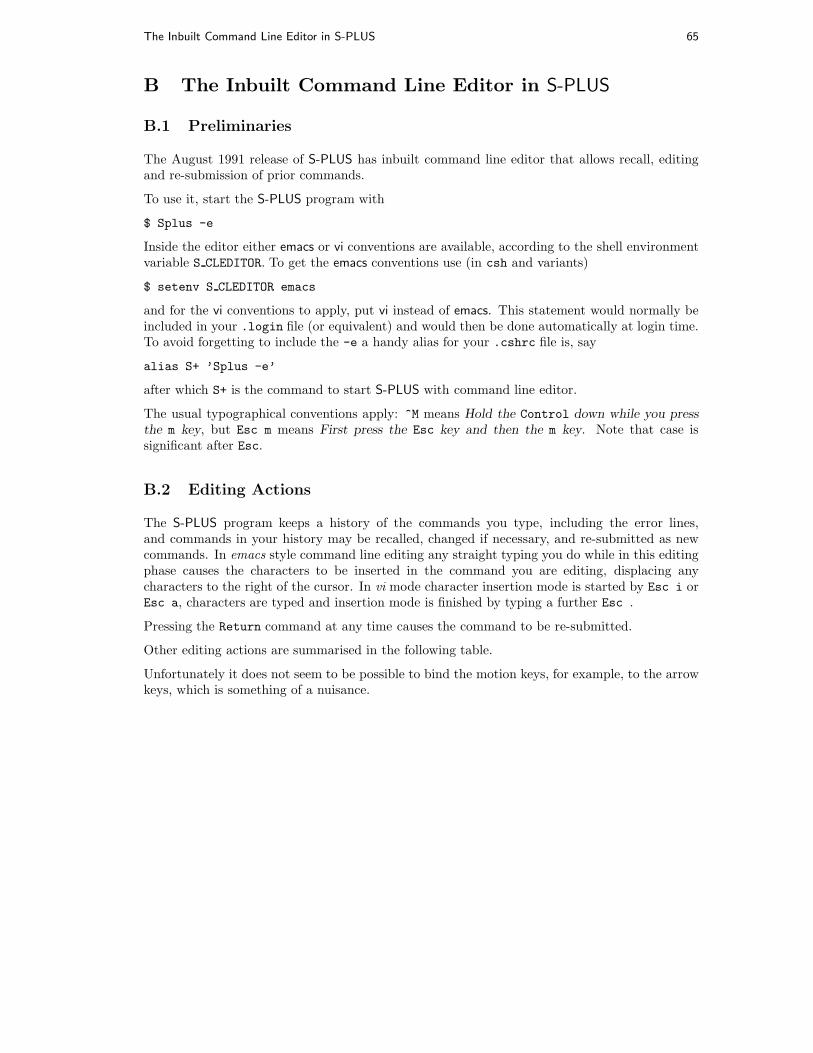
The Inbuilt Command Line Editor in S-PLUS 65

B The Inbuilt Command Line Editor in S-PLUS

B.1 Preliminaries

The August 1991 release of S-PLUS has inbuilt command line editor that allows recall, editingand re-submission of prior commands.

To use it, start the S-PLUS program with

$ Splus -e

Inside the editor either emacs or vi conventions are available, according to the shell environmentvariable S CLEDITOR. To get the emacs conventions use (in csh and variants)

$ setenv S CLEDITOR emacs

and for the vi conventions to apply, put vi instead of emacs. This statement would normally beincluded in your .login file (or equivalent) and would then be done automatically at login time.To avoid forgetting to include the -e a handy alias for your .cshrc file is, say

alias S+ ’Splus -e’

after which S+ is the command to start S-PLUS with command line editor.

The usual typographical conventions apply: ^M means Hold the Control down while you press

the m key, but Esc m means First press the Esc key and then the m key. Note that case issignificant after Esc.

B.2 Editing Actions

The S-PLUS program keeps a history of the commands you type, including the error lines,and commands in your history may be recalled, changed if necessary, and re-submitted as newcommands. In emacs style command line editing any straight typing you do while in this editingphase causes the characters to be inserted in the command you are editing, displacing anycharacters to the right of the cursor. In vi mode character insertion mode is started by Esc i orEsc a, characters are typed and insertion mode is finished by typing a further Esc .

Pressing the Return command at any time causes the command to be re-submitted.

Other editing actions are summarised in the following table.

Unfortunately it does not seem to be possible to bind the motion keys, for example, to the arrowkeys, which is something of a nuisance.

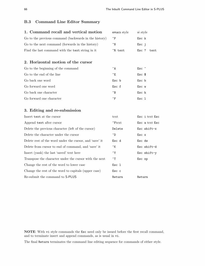
66 The Inbuilt Command Line Editor in S-PLUS

B.3 Command Line Editor Summary

1. Command recall and vertical motion emacs style vi style

Go to the previous command (backwards in the history) ^P Esc k

Go to the next command (forwards in the history) ^N Esc j

Find the last command with the text string in it ^R text Esc ? text

2. Horizontal motion of the cursor

Go to the beginning of the command ^A Esc ^

Go to the end of the line ^E Esc $

Go back one word Esc b Esc b

Go forward one word Esc f Esc w

Go back one character ^B Esc h

Go forward one character ^F Esc l

3. Editing and re-submission

Insert text at the cursor text Esc i text Esc

Append text after cursor ^Ftext Esc a text Esc

Delete the previous character (left of the cursor) Delete Esc shift-x

Delete the character under the cursor ^D Esc x

Delete rest of the word under the cursor, and ‘save’ it Esc d Esc dw

Delete from cursor to end of command, and ‘save’ it ^K Esc shift-d

Insert (yank) the last ‘saved’ text here ^Y Esc shift-y

Transpose the character under the cursor with the next ^T Esc xp

Change the rest of the word to lower case Esc l

Change the rest of the word to capitals (upper case) Esc c

Re-submit the command to S-PLUS Return Return

NOTE: With vi style commands the Esc need only be issued before the first recall command,and to terminate insert and append commands, as is usual in vi.

The final Return terminates the command line editing sequence for commands of either style.

Exercises 67

C Exercises

C.1 The cloud point data

Source: Draper & Smith, Applied Regression Analysis, p. 162Category: Polynomial regression. Simple plots.

Description

The cloud point of a liquid is a measure of the degree of crystalization in a stock that can bemeasured by the refractive index. It has been suggested that the percentage of I8 in the basestock is an excellent predictor of cloud point using the second or third order model:

Y = β0 + β1x + β2x2 + β3x

3 + E, E ∼ N(0, σ2)

Data

The following data was collected on stocks with known percentage of I8:

I8% Cloud Point I8% Cloud Point I8% Cloud Point I8% Cloud Point

0 21.9 2 26.1 5 28.9 8 31.4

0 22.1 3 26.8 6 29.8 8 31.5

0 22.8 3 27.3 6 30.0 9 31.8

1 24.5 4 28.2 6 30.3 10 33.1

2 26.0 4 28.5 7 30.4

The data may be read from file cloud.data in a form suitable to construct a data frame.

Suggested analysis

Fit polynomial regression models using the lm() function, and choose the degree carefully.

C.2 The Janka hardness data

Source: E. J. Williams: Regression Analysis, Wiley, 1959.Category: Polynomial regression. Transformations.

Description

The Janka hardness is an important structural property of Australian timbers, which is difficultto measure. It is, however, related to the density of the timber, which is relatively easy tomeasure. A low degree polynomial regression is suggested as appropriate.

Y = β0 + β1x + β2x2 + · · · + E

where Y is the hardness and x the density.

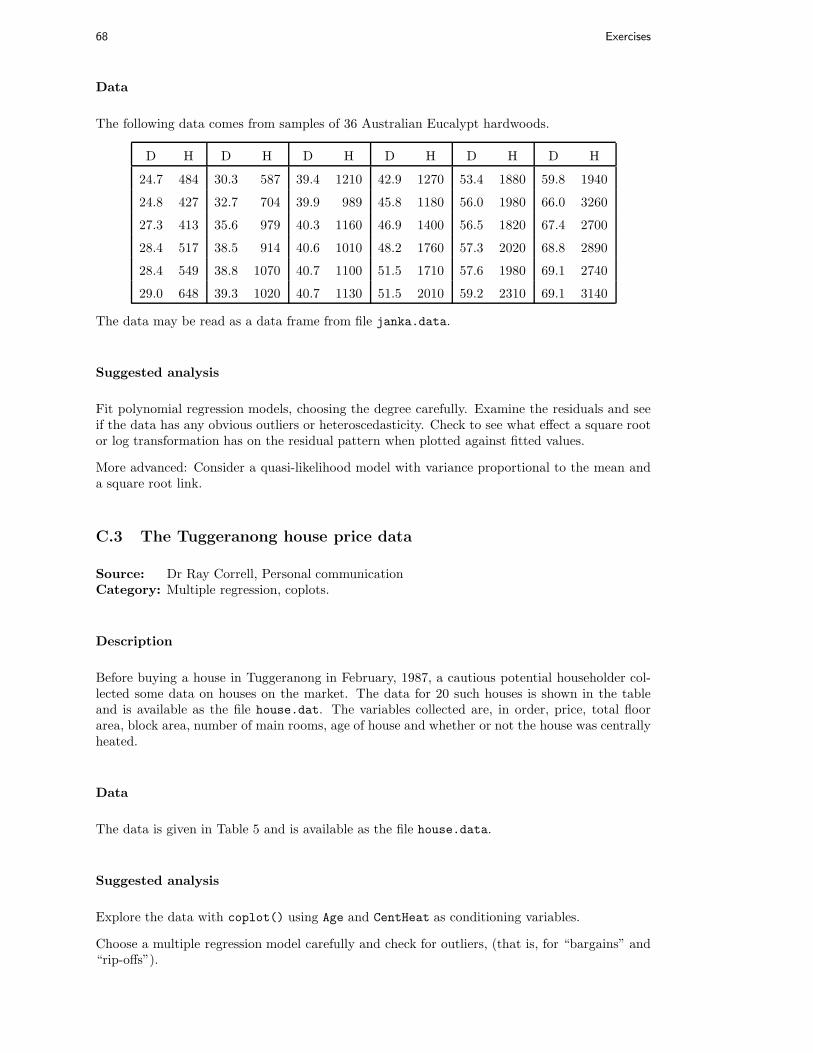
68 Exercises

Data

The following data comes from samples of 36 Australian Eucalypt hardwoods.

D H D H D H D H D H D H

24.7 484 30.3 587 39.4 1210 42.9 1270 53.4 1880 59.8 1940

24.8 427 32.7 704 39.9 989 45.8 1180 56.0 1980 66.0 3260

27.3 413 35.6 979 40.3 1160 46.9 1400 56.5 1820 67.4 2700

28.4 517 38.5 914 40.6 1010 48.2 1760 57.3 2020 68.8 2890

28.4 549 38.8 1070 40.7 1100 51.5 1710 57.6 1980 69.1 2740

29.0 648 39.3 1020 40.7 1130 51.5 2010 59.2 2310 69.1 3140

The data may be read as a data frame from file janka.data.

Suggested analysis

Fit polynomial regression models, choosing the degree carefully. Examine the residuals and seeif the data has any obvious outliers or heteroscedasticity. Check to see what effect a square rootor log transformation has on the residual pattern when plotted against fitted values.

More advanced: Consider a quasi-likelihood model with variance proportional to the mean anda square root link.

C.3 The Tuggeranong house price data

Source: Dr Ray Correll, Personal communicationCategory: Multiple regression, coplots.

Description

Before buying a house in Tuggeranong in February, 1987, a cautious potential householder col-lected some data on houses on the market. The data for 20 such houses is shown in the tableand is available as the file house.dat. The variables collected are, in order, price, total floorarea, block area, number of main rooms, age of house and whether or not the house was centrallyheated.

Data

The data is given in Table 5 and is available as the file house.data.

Suggested analysis

Explore the data with coplot() using Age and CentHeat as conditioning variables.

Choose a multiple regression model carefully and check for outliers, (that is, for “bargains” and“rip-offs”).

C.4 Yorke Penninsula wheat yield data 69

Price ($000s) Floor (m2) Block (m2) Rooms Age (years) Cent. Heat.

52.00 111.0 830 5 6.2 no

54.75 128.0 710 5 7.5 no

57.50 101.0 1000 5 4.2 no

57.50 131.0 690 6 8.8 no

59.75 93.0 900 5 1.9 yes

62.50 112.0 640 6 5.2 no

64.75 137.6 700 6 6.6 yes

67.25 148.5 740 6 2.3 no

67.50 113.5 660 6 6.1 no

69.75 152.0 645 7 9.2 no

70.00 121.5 730 5 4.3 yes

75.50 141.0 730 7 4.3 no

77.50 124.0 670 6 1.0 yes

77.50 153.5 795 7 7.0 yes

81.25 149.0 900 6 3.6 yes

82.50 135.0 810 6 1.7 yes

86.25 162.0 930 6 1.2 yes

87.50 145.0 825 6 0.0 yes

88.00 172.0 950 7 2.3 yes

92.00 170.5 870 7 0.7 yes

Table 5: The Tuggeranong house price data

C.4 Yorke Penninsula wheat yield data

Source: K. W. Morris (private communication)Category: Multiple regression.

Description

The annual yield of wheat in a marginal wheat growing district on the Yorke Penninsula, SouthAustralia, together with the rainfall for the three growing months, for the years 1931–1955. Theyear itself is potentially a surrogate predictor to allow for improvements in varieties and farmpractice. Yield is in bushels per acre, and rainfall is in inches.

Data

The data is given in Table 6 and may be read as a data frame from file sawheat.data.

Suggested analysis

Fit a multiple regression model and check the results, via residual plots especially.

70 Exercises

Year Rain0 Rain1 Rain2 Yield Year Rain0 Rain1 Rain2 Yield

1931 .05 1.61 3.52 .31 1944 3.30 4.19 2.11 4.60

1932 1.15 .60 3.46 .00 1945 .44 3.41 1.55 .35

1933 2.22 4.94 3.06 5.47 1946 .50 3.26 1.20 .00

1934 1.19 11.26 4.91 16.73 1947 .18 1.52 1.80 .00

1935 1.40 10.95 4.23 10.54 1948 .80 3.25 3.55 2.98

1936 2.96 4.96 .11 5.89 1949 7.08 5.93 .93 11.89

1937 2.68 .67 2.17 .03 1950 2.54 4.71 2.51 6.56

1938 3.66 8.49 11.95 16.03 1951 1.08 3.37 4.02 1.30

1939 5.15 3.60 2.18 6.57 1952 .22 3.24 4.93 .03

1940 6.44 2.69 1.37 8.43 1953 .55 1.78 1.97 .00

1941 2.01 6.88 .92 8.68 1954 1.65 3.22 1.65 3.09

1942 .73 3.30 3.97 2.49 1955 .72 3.42 3.31 2.72

1943 2.52 1.93 1.16 .98

Table 6: Yorke Penninsula wheat yield data

C.5 The Iowa wheat yield data

Source: CAED Report, 1964. Quoted in Draper & Smith.Category: Multiple regression; diagnostics.

Description

The data gives the pre-season and three growing months’ precipitation, the mean temperaturesfor the three growing months and harvest month, the year, and the yield of wheat for the USAstate of Iowa, for the years 1930–1962.

Data

The data is given in Table 7 and may be read as a data frame from file iowheat.data.

Suggested analysis

Fit a multiple regression model and select carefully the predictors. Work either by backwardelimination of forward selection. Examine the residuals by plotting them in turn against eachpredictor variable.

Consider the effect of adding quadratic terms in the predictors.

It is interesting to compare this set of data with the Yorke Penninsula data for a similar period.

C.6 The gasoline yield data

Source: Estimate gasoline yields from crudes

by Nilon H. Prater, Petroleum Refiner, 35, #5.Category: Analysis of variance, covariance, and multiple regression.

C.6 The gasoline yield data 71

Year Rain0 Temp1 Rain1 Temp2 Rain2 Temp3 Rain3 Temp4 Yield

1930 17.75 60.2 5.83 69.0 1.49 77.9 2.42 74.4 34.0

1931 14.76 57.5 3.83 75.0 2.72 77.2 3.30 72.6 32.9

1932 27.99 62.3 5.17 72.0 3.12 75.8 7.10 72.2 43.0

1933 16.76 60.5 1.64 77.8 3.45 76.4 3.01 70.5 40.0

1934 11.36 69.5 3.49 77.2 3.85 79.7 2.84 73.4 23.0

1935 22.71 55.0 7.00 65.9 3.35 79.4 2.42 73.6 38.4

1936 17.91 66.2 2.85 70.1 0.51 83.4 3.48 79.2 20.0

1937 23.31 61.8 3.80 69.0 2.63 75.9 3.99 77.8 44.6

1938 18.53 59.5 4.67 69.2 4.24 76.5 3.82 75.7 46.3

1939 18.56 66.4 5.32 71.4 3.15 76.2 4.72 70.7 52.2

1940 12.45 58.4 3.56 71.3 4.57 76.7 6.44 70.7 52.3

1941 16.05 66.0 6.20 70.0 2.24 75.1 1.94 75.1 51.0

1942 27.10 59.3 5.93 69.7 4.89 74.3 3.17 72.2 59.9

1943 19.05 57.5 6.16 71.6 4.56 75.4 5.07 74.0 54.7

1944 20.79 64.6 5.88 71.7 3.73 72.6 5.88 71.8 52.0

1945 21.88 55.1 4.70 64.1 2.96 72.1 3.43 72.5 43.5

1946 20.02 56.5 6.41 69.8 2.45 73.8 3.56 68.9 56.7

1947 23.17 55.6 10.39 66.3 1.72 72.8 1.49 80.6 30.5

1948 19.15 59.2 3.42 68.6 4.14 75.0 2.54 73.9 60.5

1949 18.28 63.5 5.51 72.4 3.47 76.2 2.34 73.0 46.1

1950 18.45 59.8 5.70 68.4 4.65 69.7 2.39 67.7 48.2

1951 22.00 62.2 6.11 65.2 4.45 72.1 6.21 70.5 43.1

1952 19.05 59.6 5.40 74.2 3.84 74.7 4.78 70.0 62.2

1953 15.67 60.0 5.31 73.2 3.28 74.6 2.33 73.2 52.9

1954 15.92 55.6 6.36 72.9 1.79 77.4 7.10 72.1 53.9

1955 16.75 63.6 3.07 67.2 3.29 79.8 1.79 77.2 48.4

1956 12.34 62.4 2.56 74.7 4.51 72.7 4.42 73.0 52.8

1957 15.82 59.0 4.84 68.9 3.54 77.9 3.76 72.9 62.1

1958 15.24 62.5 3.80 66.4 7.55 70.5 2.55 73.0 66.0

1959 21.72 62.8 4.11 71.5 2.29 72.3 4.92 76.3 64.2

1960 25.08 59.7 4.43 67.4 2.76 72.6 5.36 73.2 63.2

1961 17.79 57.4 3.36 69.4 5.51 72.6 3.04 72.4 75.4

1962 26.61 66.6 3.12 69.1 6.27 71.6 4.31 72.5 76.0

Table 7: The Iowa historical wheat yield data

Modern regression.

Description

The data gives the gasoline yield as a percent of crude oil, say y, and four independent variableswhich may influence yield. These are

x1: The crude oil gravity, in 0API,

72 Exercises

x2: The crude oil vapour pressure,

x3: The crude oil 10% point, ASTM,

x4: The gasoline end point.

The data comes as 10 separate samples, and within each sample the values for x1, x2, and x3 areconstant.

Data

The data is shown in Table 8, and is available as the file oil.data in a form suitable for con-structing a data frame.

Sample x1 x2 x3 x4 y Sample x1 x2 x3 x4 y

1 31.8 0.2 316 365 8.5 6 40.0 6.1 217 212 7.4

1 31.8 0.2 316 379 14.7 6 40.0 6.1 217 272 18.2

1 31.8 0.2 316 428 18.0 6 40.0 6.1 217 340 30.4

2 32.2 2.4 284 351 14.0 7 40.3 4.8 231 307 14.4

2 32.2 2.4 284 424 23.2 7 40.3 4.8 231 367 26.8

7 40.3 4.8 231 395 34.9

3 32.2 5.2 236 267 10.0 8 40.8 3.5 210 218 8.0

3 32.2 5.2 236 360 24.8 8 40.8 3.5 210 273 13.1

3 32.2 5.2 236 402 31.7 8 40.8 3.5 210 347 26.6

4 38.1 1.2 274 285 5.0 9 41.3 1.8 267 235 2.8

4 38.1 1.2 274 365 17.6 9 41.3 1.8 267 275 6.4

4 38.1 1.2 274 444 32.1 9 41.3 1.8 267 358 16.1

9 41.3 1.8 267 416 27.8

5 38.4 6.1 220 235 6.9 10 50.8 8.6 190 205 12.2

5 38.4 6.1 220 300 15.2 10 50.8 8.6 190 275 22.3

5 38.4 6.1 220 365 26.0 10 50.8 8.6 190 345 34.7

5 38.4 6.1 220 410 33.6 10 50.8 8.6 190 407 45.7

Table 8: The gasoline recovery data

Suggested analysis

Using EndPt as a covariate, check to see if differences between samples can be accounted for byregression models on the other predictors.

More advanced: Fit a two stratum ANOVA model using between and within samples as the twostrata.

C.7 The Michaelson and Morley speed of light data

Source: Weekes: A Genstat Primer.Category: Analysis of Variance.

C.8 The rat genotype data 73

Description

The classical data of Michaelson and Morley on the speed of light. The data consists of five exper-iments, each consisting of 20 consecutive “runs”. The response is the speed of light measurement,suitably coded. The data is here viewed as a randomized block experiment with experiment andrun as the factors. run may also be considered a quantitative variate to account for linear (orpolynomial) changes in the measurement over the course of a single experiment.

Data

The data is given in Table 9 and may be read as a data frame from file morley.data in a formsuitable for constructing a data frame.

Runs 1–10 Runs 11–20

E1 E2 E3 E4 E5 E1 E2 E3 E4 E5

850 960 880 890 890 1000 830 880 910 870

740 940 880 810 840 980 790 910 920 870

900 960 880 810 780 930 810 850 890 810

1070 940 860 820 810 650 880 870 860 740

930 880 720 800 760 760 880 840 880 810

850 800 720 770 810 810 830 840 720 940

950 850 620 760 790 1000 800 850 840 950

980 880 860 740 810 1000 790 840 850 800

980 900 970 750 820 960 760 840 850 810

880 840 950 760 850 960 800 840 780 870

Table 9: The Michaelson and Morley speed of light data

Suggested analysis

Using an single classification ANOVA model check for differences between experiments and sum-marise your conclusions.

C.8 The rat genotype data

Source: Quoted in Scheffe, H.: The Analysis of Variance

Category: Unbalanced double classification.

Description

Data from a foster feeding experiment with rat mothers and litters of four different genotypes:A, F , I and J . The measurement is the litter weight gain after a trial feeding period.

Data

The data is given in Table 10 and may be read as a data frame from file genotype.data.

74 Exercises

Litter’s Mother’s Genotype

Genotype A F I J

A 61.5 55.0 52.5 42.0

68.2 42.0 61.8 54.0

64.0 60.2 49.5 61.0

65.0 52.7 48.2

59.7 39.6

F 60.3 50.8 56.5 51.3

51.7 64.7 59.0 40.5

49.3 61.7 47.2

48.0 64.0 53.0

62.0

I 37.0 56.3 39.7 50.0

36.3 69.8 46.0 43.8

68.0 67.0 61.3 54.5

55.3

55.7

J 59.0 59.5 45.2 44.8

57.4 52.8 57.0 51.5

54.0 56.0 61.4 53.0

47.0 42.0

54.0

Table 10: The rat genotype data

Suggested analysis

Fit a double classificaiton model. Check for interaction using both a formal analysis and graph-ically using interaction.plot(). Test the main effects and summarise.

C.9 Fisher’s sugar beet data

Source: R. A. Fisher, Design of Experiments.Category: Analysis of variance and covariance.

Description

A classical 3×23 randomized block experiment in four blocks of size 24. The response is the totalweight of sugarbeet roots off the plot, but this is accompanied by the number of roots measured.The suggestion is that number of roots should be a covariate to allow for varying plot size.

The factors are Variety. (3 levels, a, b and c), and N, P and K each at 2 levels, present or absent.

C.10 A barley split plot field trial 75

Data

The data is given in Table 11 and may be read from the file sugar.data in a form suitable toconstruct a data frame.

Block 1 Block 2 Block 3 Block 4

V N P K No Wt No Wt No Wt No Wt

a − − − 124 162 133 162 114 127 127 158

a − − k 131 152 161 164 130 141 145 188

a − p − 115 173 134 175 134 142 109 162

a − p k 126 140 133 158 106 148 132 160

a n − − 136 184 134 178 127 168 139 199

a n − k 134 112 156 193 101 171 138 191

a n p − 132 190 104 166 119 157 132 193

a n p k 120 175 147 155 107 139 148 192

b − − − 145 133 147 130 139 138 127 128

b − − k 156 117 152 137 107 121 147 147

b − p − 152 140 138 101 125 124 120 143

b − p k 137 127 145 132 125 132 143 139

b n − − 124 163 138 159 140 166 159 174

b n − k 136 143 142 144 133 142 148 159

b n p − 140 168 142 150 133 118 138 157

b n p k 146 144 135 160 138 155 140 153

c − − − 113 122 138 132 119 123 127 146

c − − k 91 107 149 171 118 142 129 151

c − p − 123 118 139 142 127 120 124 138

c − p k 129 140 126 115 129 130 142 152

c n − − 121 118 141 152 127 149 127 165

c n − k 126 148 128 152 107 147 110 136

c n p − 103 112 144 175 102 152 143 173

c n p k 120 162 125 160 129 173 137 185

Table 11: Fisher’s sugar beet data

Suggested analysis

Analyse the data as a randomised block experiment with Wt as the response and No as a covariate.Prune the model of all unnecessary interaction terms and summarise.

C.10 A barley split plot field trial

Source: Unknown. Traditional data.

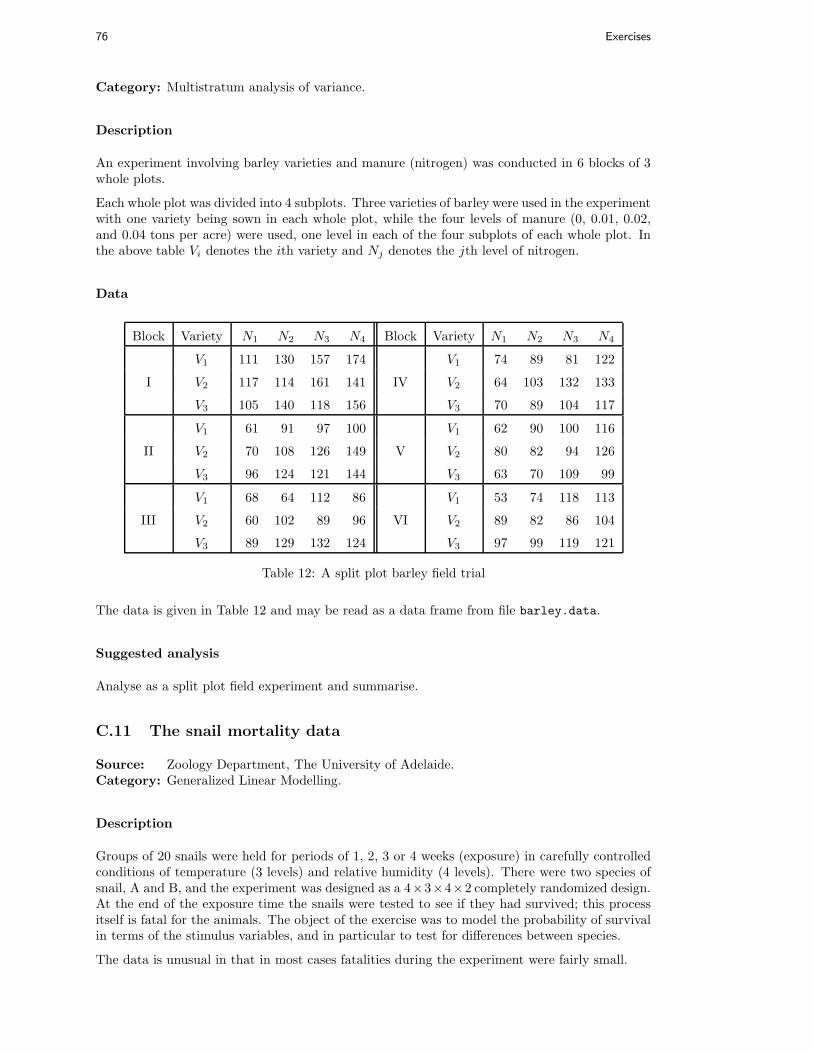
76 Exercises

Category: Multistratum analysis of variance.

Description

An experiment involving barley varieties and manure (nitrogen) was conducted in 6 blocks of 3whole plots.

Each whole plot was divided into 4 subplots. Three varieties of barley were used in the experimentwith one variety being sown in each whole plot, while the four levels of manure (0, 0.01, 0.02,and 0.04 tons per acre) were used, one level in each of the four subplots of each whole plot. Inthe above table Vi denotes the ith variety and Nj denotes the jth level of nitrogen.

Data

Block Variety N1 N2 N3 N4 Block Variety N1 N2 N3 N4

V1 111 130 157 174 V1 74 89 81 122

I V2 117 114 161 141 IV V2 64 103 132 133

V3 105 140 118 156 V3 70 89 104 117

V1 61 91 97 100 V1 62 90 100 116

II V2 70 108 126 149 V V2 80 82 94 126

V3 96 124 121 144 V3 63 70 109 99

V1 68 64 112 86 V1 53 74 118 113

III V2 60 102 89 96 VI V2 89 82 86 104

V3 89 129 132 124 V3 97 99 119 121

Table 12: A split plot barley field trial

The data is given in Table 12 and may be read as a data frame from file barley.data.

Suggested analysis

Analyse as a split plot field experiment and summarise.

C.11 The snail mortality data

Source: Zoology Department, The University of Adelaide.Category: Generalized Linear Modelling.

Description

Groups of 20 snails were held for periods of 1, 2, 3 or 4 weeks (exposure) in carefully controlledconditions of temperature (3 levels) and relative humidity (4 levels). There were two species ofsnail, A and B, and the experiment was designed as a 4×3×4×2 completely randomized design.At the end of the exposure time the snails were tested to see if they had survived; this processitself is fatal for the animals. The object of the exercise was to model the probability of survivalin terms of the stimulus variables, and in particular to test for differences between species.

The data is unusual in that in most cases fatalities during the experiment were fairly small.

C.12 The Kalythos blindness data 77

Data

Relative Humidity60.0% 65.8% 70.5% 75.8%

Temperature Temperature Temperature TemperatureSpecies Exposure 10 15 20 10 15 20 10 15 20 10 15 20

A 1 0 0 0 0 0 0 0 0 0 0 0 0

2 0 1 1 0 1 0 0 0 0 0 0 0

3 1 4 5 0 2 4 0 2 3 0 1 2

4 7 7 7 4 4 7 3 3 5 2 3 3

B 1 0 0 0 0 0 0 0 0 0 0 0 0

2 0 3 2 0 2 1 0 0 1 1 0 1

3 7 11 11 4 5 9 2 4 6 2 3 5

4 12 14 16 10 12 12 5 7 9 4 5 7

Table 13: The snail mortality data

The data is given in Table 13 and may be read as a data frame from file snails.data.

Suggested analysis

The data is intersting in that although it has many extremely small cell counts there is everyindication that some of the likelihood ratio large sample theory is quite safe.

Fit Binomial models to the data with either a logit or a probit link. Show that a model withparallel regressions on Temp, Humid, Exposure and Exposure2 for each species (in the logit/probitscale) is reasonable, and summarise.

C.12 The Kalythos blindness data

Source: S. D. Silvey: Statistical Inference. (Fictitious?)Category: Generalized linear modelling

Description

On the Greek island of Kalythos the male inhabitants suffer from a congenital eye disease, theeffects of which become more marked with increasing age. Samples of islander males of variousages were tested for blindness and the results recorded.

Data

Age: 20 35 45 55 70

No. tested: 50 50 50 50 50

No. blind: 6 17 26 37 44

Table 14: The Kalythos blindness data

The data is given in Table 14 and may be read as a data frame from file kalythos.data.

78 Exercises

Suggested analysis

Using an logit or probit model estimate the LD50, that is, the age at which the probability ofblindness is p = 1

2, together the standard error. Check how different the logit and probit models

are in this respect.

C.13 The Stormer viscometer calibration data

Source: E. J. Williams: Regression Analysis, Wiley, 1959Category: Nonlinear regression, special regression.

Description

The stormer viscometer measures the viscosity of a fluid by measuring the time taken for an innercylinder in the mechanism to perform a fixed number of revolutions in response to an actuatingweight. The viscometer is calibrated by measuring the time taken with varying weights whilethe mechanism is suspended in fluids of accurately known viscosity. The data comes from such acalibration, and theoretical considerations suggest a nonlinear relationship between time, weightand viscosity of the form

Ti =βvi

wi − θ+ Ei

where β and θ are unknown parameters to be estimated.

Data

Weight

Viscosity 20 50 100

14.7 35.6 17.6

27.5 54.3 24.3

42.0 75.6 31.4

75.7 121.2 47.2 24.6

89.7 150.8 58.3 30.0

146.6 229.0 85.6 41.7

158.3 270.0 101.1 50.3

161.1 92.2 45.1

298.3 187.2 89.0

86.5

Table 15: The Stormer viscometer calibration data

The data is given in Table 15 and may be read as a data frame from file stormer.data.

Suggested analysis

Estimate the nonlinear regression model using the nlr() software. A suitable initial value maybe obtained by writing the regression model in the form

wiTi = βvi + θTi + (wi − θ)Ei

C.14 The chlorine availability data 79

and regressing wiTi on vi and Ti using ordinary linear regression.

C.14 The chlorine availability data

Source: Draper & Smith, Applied Regression Analysis, (adapted).Category: Nonlinear regression

Description

The following set of industrial chemical data shows the amount of chlorine available in a certainproduct at various times of testing after manufacture. A nonlinear regression model for thechlorine decay of the form

Y = β0 + β1 exp(−θx)

has been suggested on theoretical grounds, with Y the amount remaining at time x.

Data

Weeks Percent available Weeks Percent available Weeks Percent available

8 49, 49 20 42, 43, 42 32 40, 41

10 47, 47, 48, 48 22 40, 41, 41 34 40

12 43, 45, 46, 46 24 40, 40, 42 36 38, 41

14 43, 43, 45 26 40, 41, 41 38 40, 40

16 43, 43, 44 28 40, 41 40 39

18 45, 46 30 38, 40, 40 42 39

Table 16: The chlorine availability data.

The data is given in Table 16 and may be read as a data frame from file chlorine.data.

Suggested analysis

Fit the nonlinear regression model using the nlr() function. A simple way to find an initialvalue is to guess a value for θ, say θ = 1 and plot Y against exp(−θx). Now repeatedly eitherdouble or halve θ until the plot is near to linear. (This can be done very simply with the inbuiltline editor.) Once an initial value for θ is available, initial values for the others can be got bylinear regression.

Check the fitted model for suspicious data points.

C.15 The saturated steam pressure data

Source: Quoted in Draper & Smith: Applied Regression Analysis. . .Category: Nonlinear regression.

80 Exercises

Description

The data gives the temperature (0C) and pressure (Pascals) in a saturated steam driven exper-imental device. The relationship between pressure, Y , and temperature, x, in saturated steamcan be written as

Y = α exp

{

βx

γ + x

}

+ E

However a more realistic model may have the experimental errors multiplicative rather thanadditive, in which case an analysis in the log scale using the model

log Y = log α +

{

βx

γ + x

}

+ E

may be more appropriate.

Data

Temp Press Temp Press Temp Press

0 4.14 50 98.76 90 522.78

10 8.52 60 151.13 95 674.32

20 16.31 70 224.74 100 782.04

30 32.18 80 341.35 105 920.01

40 64.62 85 423.36

Table 17: Temperature and pressure in saturated steam

The data is given in Table 17 and may be read as a data frame from file steam.data.

Suggested analysis

Fit both models and compare. Initial values may be got by a similar method to that employedfor the Chlorine data, since again there is only one nonlinear parameter.

C.16 Count Rumford’s friction data

Source: Bates & Watts: Nonlinear Regression Analysis. . .Category: Nonlinear regression

Description

Data on the amount of heat generated by friction was obtained by Lord Rumford in 1798. A borewas fitted into a stationary cylinder and pressed against the bottom by a screw. The bore wasturned by a team of horses for 30 minutes, after which Lord Rumford “suffered the thermometerto remain in its place nearly three quarters of an hour, observing and noting down, at smallintervals of time, the temperature indicated by it”.

Newton’s law of cooling suggests a nonlinear regression model of the form

Y = β0 + β1 exp(−θx)

where Y is the temperature and x is the time in minutes.

C.17 The jellyfish data 81

Data

Time Temp Time Temp

(min.) (0F) (min.) (0F)

4.0 126 24.0 115

5.0 125 28.0 114

7.0 123 31.0 113

12.0 120 34.0 112

14.0 119 37.5 111

16.0 118 41.0 110

20.0 116

Table 18: The Rumford friction cooling data

The data is given in Table 18 and may be read as a data frame from file rumford.data.

Suggested analysis

This data is mainly of historical interest. Handle similarly to the Chlorine data above.

C.17 The jellyfish data

Source: Interactive Statistics, Ed. Don McNeil.Category: Bivariate, two sample data.

Description

Two samples of jellyfish, from Danger Island and Salamander Bay respectively, were measuredfor length and width.

Data

The data is given in Table 19 and may be read as a data frame from file jellyfish.data.

Suggested analysis

Plot the two samples and mark in their convex hulls. Test for differences using Hotelling’s T 2.(A simple way of conducting the analysis is to regress a dummy variable for Location on Length

and width and to test the significance of both regression coefficients simultaneously.

C.18 The Archæological pottery data

Source: Tubb, A. et al. Archæometry, 22, 153–171, (1980)Category: Multivariate analysis

82 Exercises

Danger Island Salamander Bay

Width Length Width Length Width Length Width Length

6.0 9.0 11.0 13.0 12.0 14.0 16.0 20.0

6.5 8.0 11.0 14.0 13.0 17.0 16.0 20.0

6.5 9.0 11.0 14.0 14.0 16.5 16.0 21.0

7.0 9.0 12.0 13.0 14.0 19.0 16.5 19.0

7.0 10.0 13.0 14.0 15.0 16.0 17.0 20.0

7.0 11.0 14.0 16.0 15.0 17.0 18.0 19.0

8.0 9.5 15.0 16.0 15.0 18.0 18.0 19.0

8.0 10.0 15.0 16.0 15.0 18.0 18.0 20.0

8.0 10.0 15.0 19.0 15.0 19.0 19.0 20.0

8.0 11.0 16.0 16.0 15.0 21.0 19.0 22.0

9.0 11.0 16.0 18.0 20.0 22.0

10.0 13.0 16.0 19.0 21.0 21.0

Table 19: The jellyfish data – Danger Island and Salamander Bay

Description

The data arises from a chemical analysis of 26 samples of pottery found at Romano-British kilnsites in Wales, Gwent and the New Forest. The variables describe the composition, in terms ofvarious metals, and are expressed as percentages of the oxides of the metals.

The metals are aluminium, iron, magnesium, calcium and sodium and the sites are

L: Llanederyn, C: Caldicot I: Island Thorns A: Ashley Rails

Data

The data is given in Table 20 and may be read as a data frame from file pottery.data.

Suggested analysis

Investigate both numerically and graphically using a simple discriminant analysis. Exhibit thefour samples using the first two discriminant functions as coordinate axes. Summarise.

C.19 The Beaujolais quality data

Source: Quoted in Weekes: A Genstat Primer

Category: Multivariate analsysis

Description

Quality measurements for some identified samples of young Beaujolais. Extracted from Table 1in M. G. Jackson, et al : Red wine quality: correlations between colour, aroma and flavour andpigment and other parameters of young Beaujolais, Journal of Science of Food and Agriculture,29, 715–727, (1978).

C.20 The painters data of de Piles 83

Site Al Fe Mg Ca Na Site Al Fe Mg Ca Na

L 14.4 7.00 4.30 0.15 0.51 C 11.8 5.44 3.94 0.30 0.04

L 13.8 7.08 3.43 0.12 0.17 C 11.6 5.39 3.77 0.29 0.06

L 14.6 7.09 3.88 0.13 0.20 I 18.3 1.28 0.67 0.03 0.03

L 11.5 6.37 5.64 0.16 0.14 I 15.8 2.39 0.63 0.01 0.04

L 13.8 7.06 5.34 0.20 0.20 I 18.0 1.50 0.67 0.01 0.06

L 10.9 6.26 3.47 0.17 0.22 I 18.0 1.88 0.68 0.01 0.04

L 10.1 4.26 4.26 0.20 0.18 I 20.8 1.51 0.72 0.07 0.10

L 11.6 5.78 5.91 0.18 0.16 A 17.7 1.12 0.56 0.06 0.06

L 11.1 5.49 4.52 0.29 0.30 A 18.3 1.14 0.67 0.06 0.05

L 13.4 6.92 7.23 0.28 0.20 A 16.7 0.92 0.53 0.01 0.05

L 12.4 6.13 5.69 0.22 0.54 A 14.8 2.74 0.67 0.03 0.05

L 13.1 6.64 5.51 0.31 0.24 A 19.1 1.64 0.60 0.10 0.03

L 12.7 6.69 4.45 0.20 0.22

L 12.5 6.44 3.94 0.22 0.23

Table 20: The pottery composition data

Data

Label OQ AC pH TSO Label OQ AC pH TSO

A 13.54 1.51 3.36 13.8 I 12.25 1.32 3.38 1.4

B 12.58 1.35 3.15 5.2 J 14.04 1.52 3.61 4.5

C 11.83 1.09 3.30 10.6 K 12.67 1.62 3.38 0.4

D 12.83 1.15 3.41 2.2 L 13.54 1.57 3.55 7.9

E 12.83 1.32 3.44 2.3 M 13.75 1.63 3.34 6.3

F 12.12 1.23 3.31 10.5 N 9.63 0.78 3.19 40.4

G 11.29 1.14 3.49 2.5 O 12.42 1.14 3.31 3.1

H 12.79 1.22 3.56 16.7

Table 21: Quality measurements on young Beaujolais wine samples

The data is given in Table 21 and may be read as a data frame from file beaujolais.data.

Suggested analysis

Look at ways of exhibiting the data graphically. Consider a principal component analysis usingthe correlation matrix and look for any wild outliers.

C.20 The painters data of de Piles

Source: Weekes: A Genstat Primer.Category: Multivariate Analysis: Discriminant Analysis.

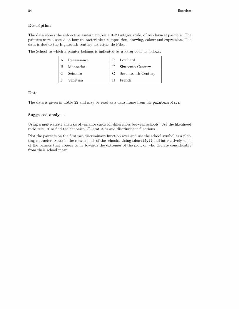
84 Exercises

Description

The data shows the subjective assessment, on a 0–20 integer scale, of 54 classical painters. Thepainters were assessed on four characteristics: composition, drawing, colour and expression. Thedata is due to the Eighteenth century art critic, de Piles.

The School to which a painter belongs is indicated by a letter code as follows:

A Renaissance E Lombard

B Mannerist F Sixteenth Century

C Seicento G Seventeenth Century

D Venetian H French

Data

The data is given in Table 22 and may be read as a data frame from file painters.data.

Suggested analysis

Using a multivariate analysis of variance check for differences between schools. Use the likelihoodratio test. Also find the canonical F−statistics and discriminant functions.

Plot the painters on the first two discriminant function axes and use the school symbol as a plot-ting character. Mark in the convex hulls of the schools. Using identify() find interactively someof the painers that appear to lie towards the extremes of the plot, or who deviate considerablyfrom their school mean.

C.20 The painters data of de Piles 85

Composition Drawing Colour Expression School

Da Udine 10 8 16 3 ADa Vinci 15 16 4 14 ADel Piombo 8 13 16 7 ADel Sarto 12 16 9 8 AFr. Penni 0 15 8 0 AGuilio Romano 15 16 4 14 AMichelangelo 8 17 4 8 APerino del Vaga 15 16 7 6 APerugino 4 12 10 4 ARaphael 17 18 12 18 A

F. Zucarro 10 13 8 8 BFr. Salviata 13 15 8 8 BParmigiano 10 15 6 6 BPrimaticcio 15 14 7 10 BT. Zucarro 13 14 10 9 BVolterra 12 15 5 8 B

Barocci 14 15 6 10 CCortona 16 14 12 6 CJosepin 10 10 6 2 CL. Jordaens 13 12 9 6 CTesta 11 15 0 6 CVanius 15 15 12 13 C

Bassano 6 8 17 0 DBellini 4 6 14 0 DGiorgione 8 9 18 4 DMurillo 6 8 15 4 DPalma Giovane 12 9 14 6 DPalma Vecchio 5 6 16 0 DPordenone 8 14 17 5 DTintoretto 15 14 16 4 DTitian 12 15 18 6 DVeronese 15 10 16 3 D

Albani 14 14 10 6 ECaravaggio 6 6 16 0 ECorregio 13 13 15 12 EDomenichino 15 17 9 17 EGuercino 18 10 10 4 ELanfranco 14 13 10 5 EThe Carraci 15 17 13 13 E

Durer 8 10 10 8 FHolbein 9 10 16 13 FPourbus 4 15 6 6 FVan Leyden 8 6 6 4 F

Diepenbeck 11 10 14 6 GJ. Jordaens 10 8 16 6 GOtho Venius 13 14 10 10 GRembrandt 15 6 17 12 GRubens 18 13 17 17 GTeniers 15 12 13 6 GVan Dyck 15 10 17 13 G

Bourdon 10 8 8 4 HLe Brun 16 16 8 16 HLe Suer 15 15 4 15 HPoussin 15 17 6 15 H

Table 22: The subjective assessment data of de Piles

Documents

Notes on S-PLUS - biostat.userweb.mwn.debiostat.userweb.mwn.de/teaching/compint2004/lit/splustutorial.pdfNotes on S-PLUS: A Programming Environment for Data Analysis and Graphics Bill