Notes on Numerical Stability

Robert A. van de GeijnThe University of Texas

Austin, TX 78712

October 10, 2014

Based on

“Goal-Oriented and Modular Stability Analysis” [3, 4]by

Paolo Bientinesi and Robert van de Geijn

NOTE: I have not thoroughly proof-read these notes!!!

1 Motivation

Correctness in the presence of error (e.g., when floating point computations are performed) takes on adifferent meaning. For many problems for which computers are used, there is one correct answer and weexpect that answer to be computed by our program. The problem is that most real numbers cannot bestored exactly in a computer memory. They are stored as approximations, floating point numbers, instead.Hence storing them and/or computing with them inherently incurs error. The question thus becomes “Whenis a program correct in the presense of such errors?”

Let us assume that we wish to evaluate the mapping f : D → R where D ⊂ Rn is the domain andR ⊂ Rm is the range (codomain). Now, we will let f : D → R denote a computer implementation of this

function. Generally, for x ∈ D it is the case that f(x) 6= f(x). Thus, the computed value is not “correct”.

From the Notes on Conditioning, we know that it may not be the case that f(x) is “close to” f(x). After

all, even if f is an exact implementation of f , the mere act of storing x may introduce a small error δx andf(x+ δx) may be far from f(x) if f is ill-conditioned.

The following defines a property that captures correctness in the presense of the kinds of errors that areintroduced by computer arithmetic:

Definition 1 Let given the mapping f : D → R, where D ⊂ Rn is the domain and R ⊂ Rm is the range(codomain), let f : D → R be a computer implementation of this function. We will call f a (numerically)

stable implementation of f on domain D if for all x ∈ D there exists a x “close” to x such that f(x) = f(x).

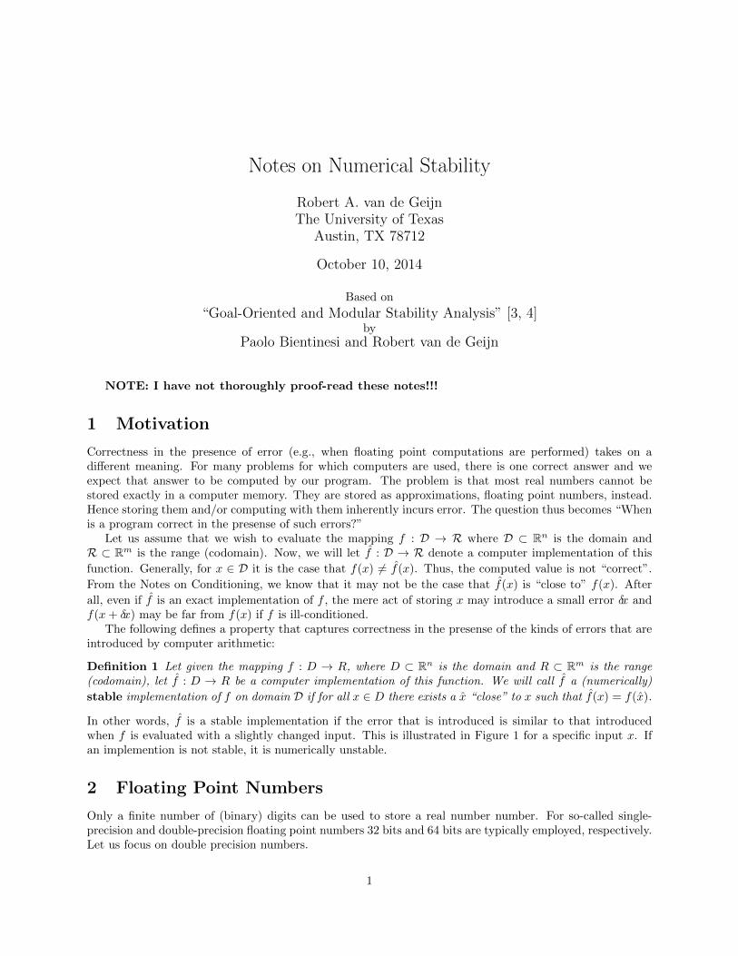
In other words, f is a stable implementation if the error that is introduced is similar to that introducedwhen f is evaluated with a slightly changed input. This is illustrated in Figure 1 for a specific input x. Ifan implemention is not stable, it is numerically unstable.

2 Floating Point Numbers

Only a finite number of (binary) digits can be used to store a real number number. For so-called single-precision and double-precision floating point numbers 32 bits and 64 bits are typically employed, respectively.Let us focus on double precision numbers.

1

Figure 1: In this illustation, f : D → R is a function to be evaluated. The function f represents theimplementation of the function that uses floating point arithmetic, thus incurring errors. The fact that for anearby value x the computed value equals the exact function applied to the slightly perturbed x, f(x) = f(x),means that the error in the computation can be attributed to a small change in the input. If this is true,then f is said to be a (numerically) stable implementation of f for input x.

Recall that any real number can be written as µ× βe, where β is the base (an integer greater than one),µ ∈ (−1, 1) is the mantissa, and e is the exponent (an integer). For our discussion, we will define F as theset of all numbers χ = µβe such that β = 2, µ = ±.δ0δ1 · · · δt−1 has only t (binary) digits (δj ∈ {0, 1}),δ0 = 0 iff µ = 0 (the mantissa is normalized), and −L ≤ e ≤ U . Elements in F can be stored with a finitenumber of (binary) digits.

• There is a largest number (in absolute value) that can be stored. Any number that is larger “overflows”.Typically, this causes a value that denotes a NaN (Not-a-Number) to be stored.

• There is a smallest number (in absolute value) that can be stored. Any number that is smaller“underflows”. Typically, this causes a zero to be stored.

Example 2 For x ∈ Rn, consider computing

‖x‖2 =

√√√√n−1∑i=0

χ2i . (1)

Notice that‖x‖2 ≤

√nn−1maxi=0|χi|

2

and hence unless some χi is close to overflowing, the result will not overflow. The problem is that if someelement χi has the property that χ2

i overflows, intermediate results in the computation in (1) will overflow.The solution is to determine k such that

|χk| = maxn−1i=0 |χi|

and to then instead compute

‖x‖2 = |χk|

√√√√n−1∑i=0

(χiχk

)2

.

It can be argued that the same approach also avoids underflow if underflow can be avoided..

In our further discussions, we will ignore overflow and underflow issues.What is important is that any time a real number is stored in our computer, it is stored as the nearest

floating point number (element in F ). We first assume that it is truncated (which makes our explanationslightly simpler).

Let positive χ be represented byχ = .δ0δ1 · · · × 2e,

where δ0 = 1 (the mantissa is normalized). If t digits are stored by our floating point system, then χ =.δ0δ1 · · · δt−1 × 2e is stored. Let δχ = χ− χ. Then

δχ = .δ0δ1 · · · δt−1δt · · · × 2e︸ ︷︷ ︸χ

− .δ0δ1 · · · δt−1 × 2e︸ ︷︷ ︸χ

= .0 · · · 0︸ ︷︷ ︸t

δt · · · × 2e < .0 · · · 01︸ ︷︷ ︸t

× 2e = 2e−t.

Also, since χ is positive,χ = .δ0δ1 · · · × 2e ≥ .1× 2e ≥ 2e−1.

Thus,δχ

χ≤ 2e−t

2e−1= 21−t

which can also be written asδχ ≤ 21−tχ.

A careful analysis of what happens when χ might equal zero or be negative yields

|δχ| ≤ 21−t|χ|.

Now, in practice any base β can be used and floating point computation uses rounding rather thantruncating. A similar analysis can be used to show that then

|δχ| ≤ u|χ|

where u = 12β

1−t is known as the machine epsilon or unit roundoff. When using single precision ordouble precision real arithmetic, u ≈ 10−8 or 10−16, respectively. The quantity u is machine dependent; it isa function of the parameters characterizing the machine arithmetic. The unit roundoff is often alternativelydefined as the maximum positive floating point number which can be added to the number stored as 1without changing the number stored as 1. In the notation introduced below, [1 + u] = 1.

Exercise 3 Assume a floating point number system with β = 2 and a mantissa with t digits so that a typicalpositive number is written as .d0d1 . . . dt−1 × 2e, with di ∈ {0, 1}.

3

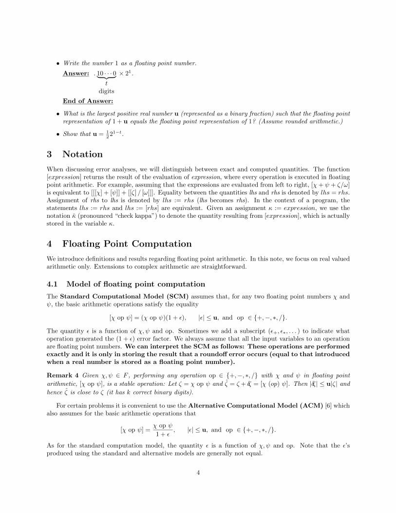
• Write the number 1 as a floating point number.

Answer: . 10 · · · 0︸ ︷︷ ︸t

digits

× 21.

End of Answer:

• What is the largest positive real number u (represented as a binary fraction) such that the floating pointrepresentation of 1 + u equals the floating point representation of 1? (Assume rounded arithmetic.)

• Show that u = 1221−t.

3 Notation

When discussing error analyses, we will distinguish between exact and computed quantities. The function[expression] returns the result of the evaluation of expression, where every operation is executed in floatingpoint arithmetic. For example, assuming that the expressions are evaluated from left to right, [χ+ ψ + ζ/ω]is equivalent to [[[χ] + [ψ]] + [[ζ] / [ω]]]. Equality between the quantities lhs and rhs is denoted by lhs = rhs.Assignment of rhs to lhs is denoted by lhs := rhs (lhs becomes rhs). In the context of a program, thestatements lhs := rhs and lhs := [rhs] are equivalent. Given an assignment κ := expression, we use thenotation κ (pronounced “check kappa”) to denote the quantity resulting from [expression], which is actuallystored in the variable κ.

4 Floating Point Computation

We introduce definitions and results regarding floating point arithmetic. In this note, we focus on real valuedarithmetic only. Extensions to complex arithmetic are straightforward.

4.1 Model of floating point computation

The Standard Computational Model (SCM) assumes that, for any two floating point numbers χ andψ, the basic arithmetic operations satisfy the equality

[χ op ψ] = (χ op ψ)(1 + ε), |ε| ≤ u, and op ∈ {+,−, ∗, /}.

The quantity ε is a function of χ, ψ and op. Sometimes we add a subscript (ε+, ε∗, . . . ) to indicate whatoperation generated the (1 + ε) error factor. We always assume that all the input variables to an operationare floating point numbers. We can interpret the SCM as follows: These operations are performedexactly and it is only in storing the result that a roundoff error occurs (equal to that introducedwhen a real number is stored as a floating point number).

Remark 4 Given χ, ψ ∈ F , performing any operation op ∈ {+,−, ∗, /} with χ and ψ in floating point

arithmetic, [χ op ψ], is a stable operation: Let ζ = χ op ψ and ζ = ζ + δζ = [χ (op) ψ]. Then |δζ| ≤ u|ζ| and

hence ζ is close to ζ (it has k correct binary digits).

For certain problems it is convenient to use the Alternative Computational Model (ACM) [6] whichalso assumes for the basic arithmetic operations that

[χ op ψ] =χ op ψ

1 + ε, |ε| ≤ u, and op ∈ {+,−, ∗, /}.

As for the standard computation model, the quantity ε is a function of χ, ψ and op. Note that the ε’sproduced using the standard and alternative models are generally not equal.

4

Remark 5 Notice that the Taylor series expansion of 1/(1 + ε) is given by

1

1 + ε= 1 + (−ε) +O(ε2),

which explains how the SCM and ACM are related.

Remark 6 Sometimes it is more convenient to use the SCM and sometimes the ACM. Trial and error, andeventually experience, will determine which one to use.

4.2 Stability of a numerical algorithm

In the presence of round-off error, an algorithm involving numerical computations cannot be expected toyield the exact result. Thus, the notion of “correctness” applies only to the execution of algorithms in exactarithmetic. Here we briefly introduce the notion of “stability” of algorithms.

Let f : D → R be a mapping from the domain D to the range R and let f : D → R represent themapping that captures the execution in floating point arithmetic of a given algorithm which computes f .

The algorithm is said to be backward stable if for all x ∈ D there exists a perturbed input x ∈ D,close to x, such that f(x) = f(x). In other words, the computed result equals the result obtained when theexact function is applied to slightly perturbed data. The difference between x and x, δx = x − x, is theperturbation to the original input x.

The reasoning behind backward stability is as follows. The input to a function typically has some errorsassociated with it. Uncertainty may be due to measurement errors when obtaining the input and/or maybe the result of converting real numbers to floating point numbers when storing the input on a computer.If it can be shown that an implementation is backward stable, then it has been proved that the result couldhave been obtained through exact computations performed on slightly corrupted input. Thus, one can thinkof the error introduced by the implementation as being comparable to the error introduced when obtainingthe input data in the first place.

When discussing error analyses, δx, the difference between x and x, is the backward error and thedifference f(x)−f(x) is the forward error. Throughout the remainder of this note we will be concerned withbounding the backward and/or forward errors introduced by the algorithms executed with floating pointarithmetic.

The algorithm is said to be forward stable on domain D if for all x ∈ D it is that case that f(x) ≈ f(x).In other words, the computed result equals a slight perturbation of the exact result.

4.3 Absolute value of vectors and matrices

In the above discussion of error, the vague notions of “near” and “slightly perturbed” are used. Makingthese notions exact usually requires the introduction of measures of size for vectors and matrices, i.e., norms.Instead, for the operations analyzed in this note, all bounds are given in terms of the absolute values ofthe individual elements of the vectors and/or matrices. While it is easy to convert such bounds to boundsinvolving norms, the converse is not true.

Definition 7 Given x ∈ Rn and A ∈ Rm×n,

|x| =

|χ0||χ1|

...|χn−1|

and |A| =

|α0,0| |α0,1| . . . |α0,n−1||α1,0| |α1,1| . . . |α1,n−1|

......

. . ....

|αm−1,0| |αm−1,1| . . . |αm−1,n−1|

.Definition 8 Let M∈{<,≤,=,≥, >} and x, y ∈ Rn. Then

|x|M |y| iff |χi|M |ψi|,

5

with i = 0, . . . , n− 1. Similarly, given A and B ∈ Rm×n,

|A|M |B| iff |αij |M |βij |,

with i = 0, . . . ,m− 1 and j = 0, . . . , n− 1.

The next Lemma is exploited in later sections:

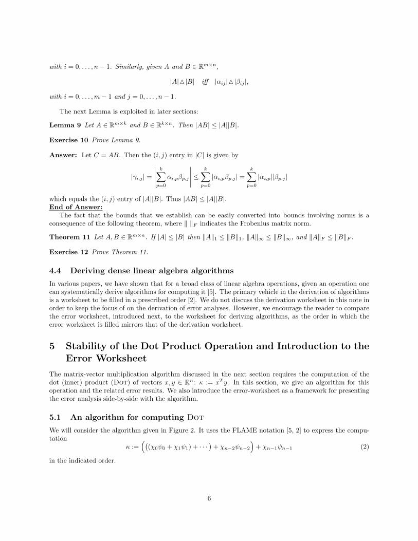
Lemma 9 Let A ∈ Rm×k and B ∈ Rk×n. Then |AB| ≤ |A||B|.

Exercise 10 Prove Lemma 9.

Answer: Let C = AB. Then the (i, j) entry in |C| is given by

|γi,j | =

∣∣∣∣∣k∑p=0

αi,pβp,j

∣∣∣∣∣ ≤k∑p=0

|αi,pβp,j | =k∑p=0

|αi,p||βp,j |

which equals the (i, j) entry of |A||B|. Thus |AB| ≤ |A||B|.End of Answer:

The fact that the bounds that we establish can be easily converted into bounds involving norms is aconsequence of the following theorem, where ‖ ‖F indicates the Frobenius matrix norm.

Theorem 11 Let A,B ∈ Rm×n. If |A| ≤ |B| then ‖A‖1 ≤ ‖B‖1, ‖A‖∞ ≤ ‖B‖∞, and ‖A‖F ≤ ‖B‖F .

Exercise 12 Prove Theorem 11.

4.4 Deriving dense linear algebra algorithms

In various papers, we have shown that for a broad class of linear algebra operations, given an operation onecan systematically derive algorithms for computing it [5]. The primary vehicle in the derivation of algorithmsis a worksheet to be filled in a prescribed order [2]. We do not discuss the derivation worksheet in this note inorder to keep the focus of on the derivation of error analyses. However, we encourage the reader to comparethe error worksheet, introduced next, to the worksheet for deriving algorithms, as the order in which theerror worksheet is filled mirrors that of the derivation worksheet.

5 Stability of the Dot Product Operation and Introduction to theError Worksheet

The matrix-vector multiplication algorithm discussed in the next section requires the computation of thedot (inner) product (Dot) of vectors x, y ∈ Rn: κ := xT y. In this section, we give an algorithm for thisoperation and the related error results. We also introduce the error-worksheet as a framework for presentingthe error analysis side-by-side with the algorithm.

5.1 An algorithm for computing Dot

We will consider the algorithm given in Figure 2. It uses the FLAME notation [5, 2] to express the compu-tation

κ :=((

(χ0ψ0 + χ1ψ1) + · · ·)

+ χn−2ψn−2

)+ χn−1ψn−1 (2)

in the indicated order.

6

Algorithm Dot: κ := xT y

κ := 0

Partition x→(xTxB

), y →

(yTyB

)where xT and yT are empty

While m(xT ) < m(x) do

Repartition(xTxB

)→

x0

χ1

x2

,

(yTyB

)→

y0

ψ1

y2

where χ1 and ψ1 are scalars

κ := κ+ χ1ψ1

Continue with(xTxB

)←

x0

χ1

x2

,

(yTyB

)←

y0

ψ1

y2

endwhile

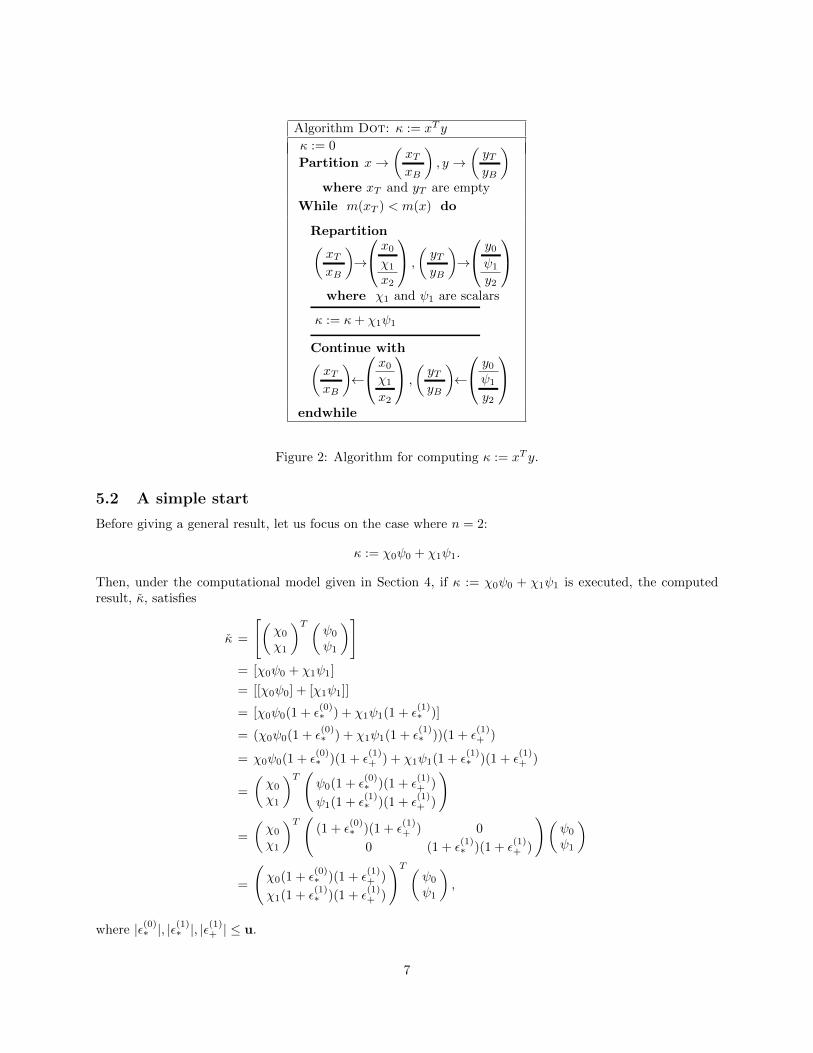
Figure 2: Algorithm for computing κ := xT y.

5.2 A simple start

Before giving a general result, let us focus on the case where n = 2:

κ := χ0ψ0 + χ1ψ1.

Then, under the computational model given in Section 4, if κ := χ0ψ0 + χ1ψ1 is executed, the computedresult, κ, satisfies

κ =

[(χ0

χ1

)T (ψ0

ψ1

)]= [χ0ψ0 + χ1ψ1]

= [[χ0ψ0] + [χ1ψ1]]

= [χ0ψ0(1 + ε(0)∗ ) + χ1ψ1(1 + ε

(1)∗ )]

= (χ0ψ0(1 + ε(0)∗ ) + χ1ψ1(1 + ε

(1)∗ ))(1 + ε

(1)+ )

= χ0ψ0(1 + ε(0)∗ )(1 + ε

(1)+ ) + χ1ψ1(1 + ε

(1)∗ )(1 + ε

(1)+ )

=

(χ0

χ1

)T (ψ0(1 + ε

(0)∗ )(1 + ε

(1)+ )

ψ1(1 + ε(1)∗ )(1 + ε

(1)+ )

)

=

(χ0

χ1

)T ((1 + ε

(0)∗ )(1 + ε

(1)+ ) 0

0 (1 + ε(1)∗ )(1 + ε

(1)+ )

)(ψ0

ψ1

)

=

(χ0(1 + ε

(0)∗ )(1 + ε

(1)+ )

χ1(1 + ε(1)∗ )(1 + ε

(1)+ )

)T (ψ0

ψ1

),

where |ε(0)∗ |, |ε(1)

∗ |, |ε(1)+ | ≤ u.

7

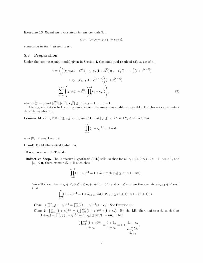
Exercise 13 Repeat the above steps for the computation

κ := ((χ0ψ0 + χ1ψ1) + χ2ψ2),

computing in the indicated order.

5.3 Preparation

Under the computational model given in Section 4, the computed result of (2), κ, satisfies

κ =

(((χ0ψ0(1 + ε

(0)∗ ) + χ1ψ1(1 + ε

(1)∗ ))(1 + ε

(1)+ ) + · · ·

)(1 + ε

(n−2)+ )

+ χn−1ψn−1(1 + ε(n−1)∗ )

)(1 + ε

(n−1)+ )

=

n−1∑i=0

χiψi(1 + ε(i)∗ )

n−1∏j=i

(1 + ε(j)+ )

, (3)

where ε(0)+ = 0 and |ε(0)

∗ |, |ε(j)∗ |, |ε(j)+ | ≤ u for j = 1, . . . , n− 1.Clearly, a notation to keep expressions from becoming unreadable is desirable. For this reason we intro-

duce the symbol θj :

Lemma 14 Let εi ∈ R, 0 ≤ i ≤ n− 1, nu < 1, and |εi| ≤ u. Then ∃ θn ∈ R such that

n−1∏i=0

(1 + εi)±1 = 1 + θn,

with |θn| ≤ nu/(1− nu).

Proof: By Mathematical Induction.

Base case. n = 1. Trivial.

Inductive Step. The Inductive Hypothesis (I.H.) tells us that for all εi ∈ R, 0 ≤ i ≤ n− 1, nu < 1, and|εi| ≤ u, there exists a θn ∈ R such that

n−1∏i=0

(1 + εi)±1 = 1 + θn, with |θn| ≤ nu/(1− nu).

We will show that if εi ∈ R, 0 ≤ i ≤ n, (n + 1)u < 1, and |εi| ≤ u, then there exists a θn+1 ∈ R suchthat

n∏i=0

(1 + εi)±1 = 1 + θn+1, with |θn+1| ≤ (n+ 1)u/(1− (n+ 1)u).

Case 1:∏ni=0(1 + εi)

±1 =∏n−1i=0 (1 + εi)

±1(1 + εn). See Exercise 15.

Case 2:∏ni=0(1 + εi)

±1 = (∏n−1i=0 (1 + εi)

±1)/(1 + εn). By the I.H. there exists a θn such that

(1 + θn) =∏n−1i=0 (1 + εi)

±1 and |θn| ≤ nu/(1− nu). Then∏n−1i=0 (1 + εi)

±1

1 + εn=

1 + θn1 + εn

= 1 +θn − εn1 + εn︸ ︷︷ ︸θn+1

,

8

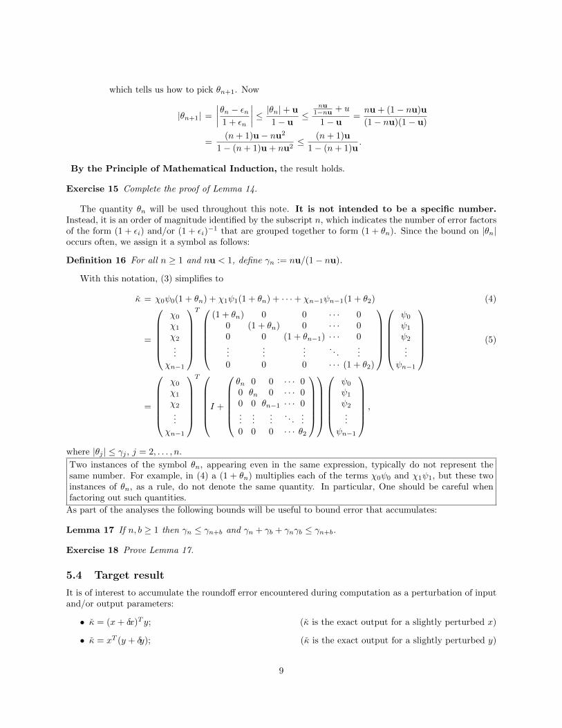
which tells us how to pick θn+1. Now

|θn+1| =

∣∣∣∣θn − εn1 + εn

∣∣∣∣ ≤ |θn|+ u

1− u≤

nu1−nu + u

1− u=nu + (1− nu)u

(1− nu)(1− u)

=(n+ 1)u− nu2

1− (n+ 1)u + nu2≤ (n+ 1)u

1− (n+ 1)u.

By the Principle of Mathematical Induction, the result holds.

Exercise 15 Complete the proof of Lemma 14.

The quantity θn will be used throughout this note. It is not intended to be a specific number.Instead, it is an order of magnitude identified by the subscript n, which indicates the number of error factorsof the form (1 + εi) and/or (1 + εi)

−1 that are grouped together to form (1 + θn). Since the bound on |θn|occurs often, we assign it a symbol as follows:

Definition 16 For all n ≥ 1 and nu < 1, define γn := nu/(1− nu).

With this notation, (3) simplifies to

κ = χ0ψ0(1 + θn) + χ1ψ1(1 + θn) + · · ·+ χn−1ψn−1(1 + θ2) (4)

=

χ0

χ1

χ2

...χn−1

T

(1 + θn) 0 0 · · · 00 (1 + θn) 0 · · · 00 0 (1 + θn−1) · · · 0...

......

. . ....

0 0 0 · · · (1 + θ2)

ψ0

ψ1

ψ2

...ψn−1

(5)

=

χ0

χ1

χ2

...χn−1

T I +

θn 0 0 · · · 00 θn 0 · · · 00 0 θn−1 · · · 0...

......

. . ....

0 0 0 · · · θ2

ψ0

ψ1

ψ2

...ψn−1

,

where |θj | ≤ γj , j = 2, . . . , n.

Two instances of the symbol θn, appearing even in the same expression, typically do not represent thesame number. For example, in (4) a (1 + θn) multiplies each of the terms χ0ψ0 and χ1ψ1, but these twoinstances of θn, as a rule, do not denote the same quantity. In particular, One should be careful whenfactoring out such quantities.

As part of the analyses the following bounds will be useful to bound error that accumulates:

Lemma 17 If n, b ≥ 1 then γn ≤ γn+b and γn + γb + γnγb ≤ γn+b.

Exercise 18 Prove Lemma 17.

5.4 Target result

It is of interest to accumulate the roundoff error encountered during computation as a perturbation of inputand/or output parameters:

• κ = (x+ δx)T y; (κ is the exact output for a slightly perturbed x)

• κ = xT (y + δy); (κ is the exact output for a slightly perturbed y)

9

• κ = xT y + δκ. (κ equals the exact result plus an error)

The first two are backward error results (error is accumulated onto input parameters, showing that thealgorithm is numerically stable since it yields the exact output for a slightly perturbed input) while the lastone is a forward error result (error is accumulated onto the answer). We will see that in different situations,a different error result may be needed by analyses of operations that require a dot product.

Let us focus on the second result. Ideally one would show that each of the entries of y is slightly perturbedrelative to that entry:

δy =

σ0ψ0

...σn−1ψn−1

=

σ0 · · · 0...

. . ....

0 · · · σn−1

ψ0

...ψn−1

= Σy,

where each σi is “small” and Σ = diag(σ0, . . . , σn−1). The following special structure of Σ, inspired by (5)will be used in the remainder of this note:

Σ(n) =

0× 0 matrix if n = 0θ1 if n = 1diag(θn, θn, θn−1, . . . , θ2) otherwise.

(6)

Recall that θj is an order of magnitude variable with |θj | ≤ γj .

Exercise 19 Let k ≥ 0 and assume that |ε1|, |ε2| ≤ u, with ε1 = 0 if k = 0. Show that(I + Σ(k) 0

0 (1 + ε1)

)(1 + ε2) = (I + Σ(k+1)).

Hint: reason the case where k = 0 separately from the case where k > 0.

We state a theorem that captures how error is accumulated by the algorithm.

Theorem 20 Let x, y ∈ Rn and let κ := xT y be computed by executing the algorithm in Figure 2. Then

κ =[xT y

]= xT (I + Σ(n))y.

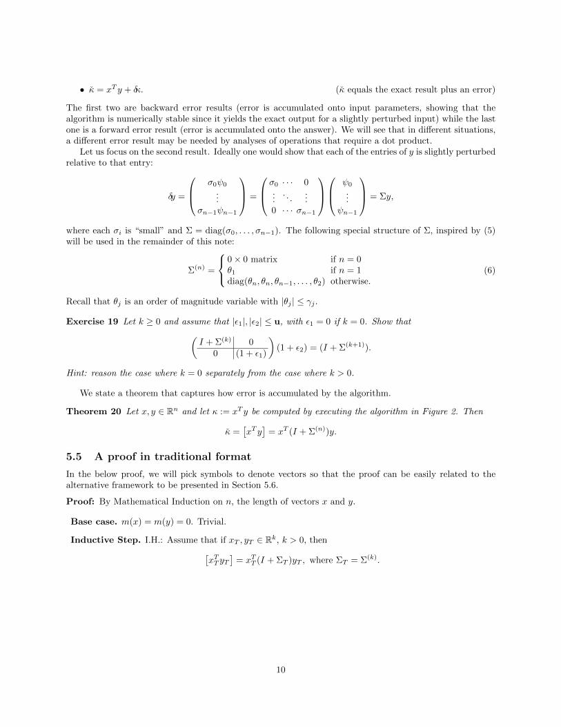
5.5 A proof in traditional format

In the below proof, we will pick symbols to denote vectors so that the proof can be easily related to thealternative framework to be presented in Section 5.6.

Proof: By Mathematical Induction on n, the length of vectors x and y.

Base case. m(x) = m(y) = 0. Trivial.

Inductive Step. I.H.: Assume that if xT , yT ∈ Rk, k > 0, then[xTT yT

]= xTT (I + ΣT )yT , where ΣT = Σ(k).

10

We will show that when xT , yT ∈ Rk+1, the equality[xTT yT

]= xTT (I+ΣT )yT holds true again. Assume

that xT , yT ∈ Rk+1, and partition xT →(x0

χ1

)and yT →

(y0

ψ1

). Then

[(x0

χ1

)T (y0

ψ1

)]=[[xT0 y0

]+ [χ1ψ1]

](definition)

=[xT0 (I + Σ0)y0 + [χ1ψ1]

](I.H. with xT = x0,

yT = y0, and Σ0 = Σ(k))

=(xT0 (I + Σ0)y0 + χ1ψ1(1 + ε∗)

)(1 + ε+) (SCM, twice)

=

(x0

χ1

)T ((I + Σ0) 0

0 (1 + ε∗)

)(1 + ε+)

(y0

ψ1

)(rearrangement)

= xTT (I + ΣT )yT (renaming),

where |ε∗|, |ε+| ≤ u, ε+ = 0 if k = 0, and (I+ΣT ) =

((I + Σ0) 0

0 (1 + ε∗)

)(1+ε+) so that ΣT = Σ(k+1).

By the Principle of Mathematical Induction, the result holds.

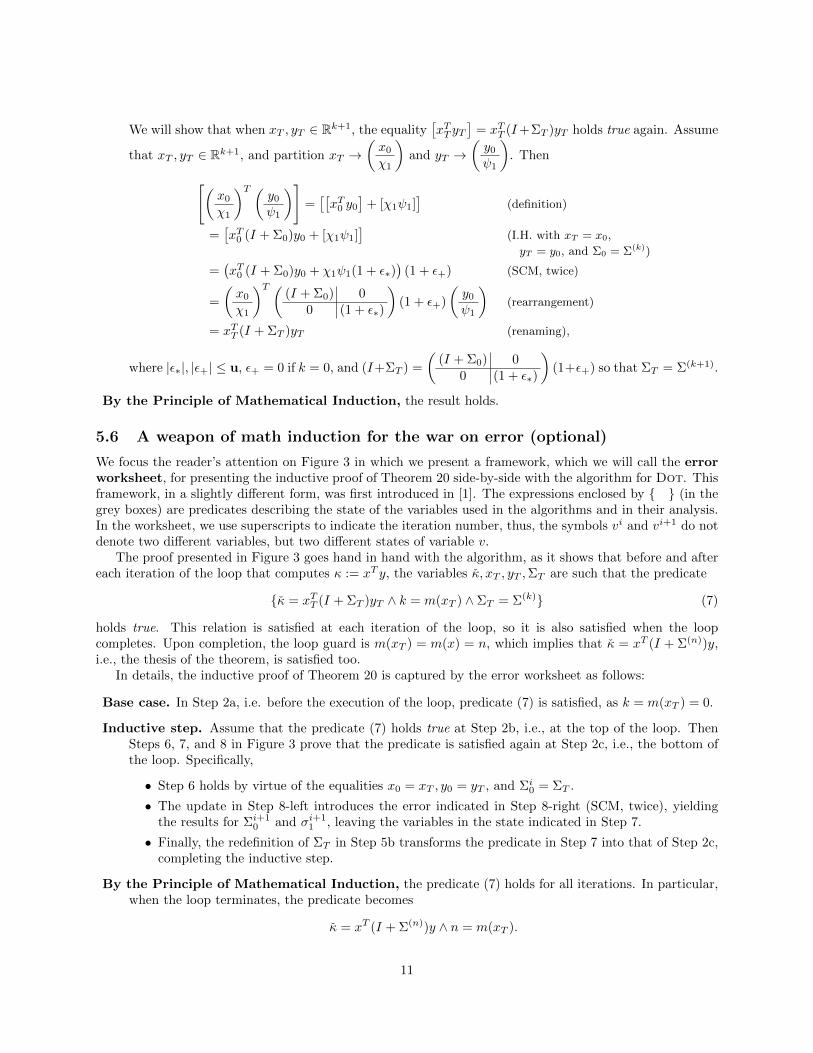
5.6 A weapon of math induction for the war on error (optional)

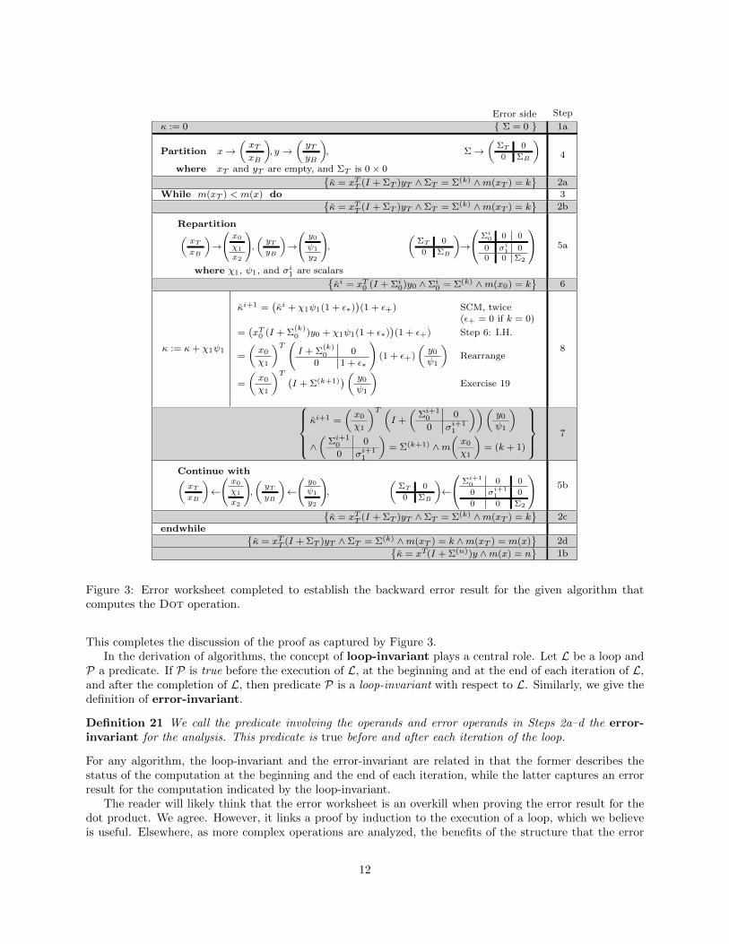
We focus the reader’s attention on Figure 3 in which we present a framework, which we will call the errorworksheet, for presenting the inductive proof of Theorem 20 side-by-side with the algorithm for Dot. Thisframework, in a slightly different form, was first introduced in [1]. The expressions enclosed by { } (in thegrey boxes) are predicates describing the state of the variables used in the algorithms and in their analysis.In the worksheet, we use superscripts to indicate the iteration number, thus, the symbols vi and vi+1 do notdenote two different variables, but two different states of variable v.

The proof presented in Figure 3 goes hand in hand with the algorithm, as it shows that before and aftereach iteration of the loop that computes κ := xT y, the variables κ, xT , yT ,ΣT are such that the predicate

{κ = xTT (I + ΣT )yT ∧ k = m(xT ) ∧ ΣT = Σ(k)} (7)

holds true. This relation is satisfied at each iteration of the loop, so it is also satisfied when the loopcompletes. Upon completion, the loop guard is m(xT ) = m(x) = n, which implies that κ = xT (I + Σ(n))y,i.e., the thesis of the theorem, is satisfied too.

In details, the inductive proof of Theorem 20 is captured by the error worksheet as follows:

Base case. In Step 2a, i.e. before the execution of the loop, predicate (7) is satisfied, as k = m(xT ) = 0.

Inductive step. Assume that the predicate (7) holds true at Step 2b, i.e., at the top of the loop. ThenSteps 6, 7, and 8 in Figure 3 prove that the predicate is satisfied again at Step 2c, i.e., the bottom ofthe loop. Specifically,

• Step 6 holds by virtue of the equalities x0 = xT , y0 = yT , and Σi0 = ΣT .

• The update in Step 8-left introduces the error indicated in Step 8-right (SCM, twice), yieldingthe results for Σi+1

0 and σi+11 , leaving the variables in the state indicated in Step 7.

• Finally, the redefinition of ΣT in Step 5b transforms the predicate in Step 7 into that of Step 2c,completing the inductive step.

By the Principle of Mathematical Induction, the predicate (7) holds for all iterations. In particular,when the loop terminates, the predicate becomes

κ = xT (I + Σ(n))y ∧ n = m(xT ).

11

Error side Step

κ := 0 { Σ = 0 } 1a

Partition x→(xTxB

), y →

(yTyB

), Σ→

(ΣT 0

0 ΣB

)where xT and yT are empty, and ΣT is 0× 0

4

{κ = xTT (I + ΣT )yT ∧ ΣT = Σ(k) ∧m(xT ) = k

}2a

While m(xT ) < m(x) do 3{κ = xTT (I + ΣT )yT ∧ ΣT = Σ(k) ∧m(xT ) = k

}2b

Repartition(xT

xB

)→

x0

χ1

x2

,( yTyB

)→

y0ψ1

y2

, (ΣT 0

0 ΣB

)→

Σi0 0 0

0 σi1 0

0 0 Σ2

where χ1, ψ1, and σi

1 are scalars

5a

{κi = xT0 (I + Σi

0)y0 ∧ Σi0 = Σ(k) ∧m(x0) = k

}6

κ := κ+ χ1ψ1

κi+1 =(κi + χ1ψ1(1 + ε∗)

)(1 + ε+) SCM, twice

(ε+ = 0 if k = 0)

=(xT0 (I + Σ

(k)0 )y0 + χ1ψ1(1 + ε∗)

)(1 + ε+) Step 6: I.H.

=

(x0χ1

)T(I + Σ

(k)0 0

0 1 + ε∗

)(1 + ε+)

(y0ψ1

)Rearrange

=

(x0χ1

)T (I + Σ(k+1)

)( y0ψ1

)Exercise 19

8

κi+1 =

(x0χ1

)T (I +

(Σi+1

0 0

0 σi+11

))(y0ψ1

)∧(

Σi+10 0

0 σi+11

)= Σ(k+1) ∧m

(x0χ1

)= (k + 1)

7

Continue with(xT

xB

)←(x0

χ1

x2

),

(yTyB

)←(y0ψ1

y2

),

(ΣT 0

0 ΣB

)←

Σi+10 0 0

0 σi+11 0

0 0 Σ2

5b

{κ = xTT (I + ΣT )yT ∧ ΣT = Σ(k) ∧m(xT ) = k

}2c

endwhile {κ = xTT (I + ΣT )yT ∧ ΣT = Σ(k) ∧m(xT ) = k ∧m(xT ) = m(x)

}2d{

κ = xT(I + Σ(n))y ∧m(x) = n}

1b

Figure 3: Error worksheet completed to establish the backward error result for the given algorithm thatcomputes the Dot operation.

This completes the discussion of the proof as captured by Figure 3.In the derivation of algorithms, the concept of loop-invariant plays a central role. Let L be a loop and

P a predicate. If P is true before the execution of L, at the beginning and at the end of each iteration of L,and after the completion of L, then predicate P is a loop-invariant with respect to L. Similarly, we give thedefinition of error-invariant.

Definition 21 We call the predicate involving the operands and error operands in Steps 2a–d the error-invariant for the analysis. This predicate is true before and after each iteration of the loop.

For any algorithm, the loop-invariant and the error-invariant are related in that the former describes thestatus of the computation at the beginning and the end of each iteration, while the latter captures an errorresult for the computation indicated by the loop-invariant.

The reader will likely think that the error worksheet is an overkill when proving the error result for thedot product. We agree. However, it links a proof by induction to the execution of a loop, which we believeis useful. Elsewhere, as more complex operations are analyzed, the benefits of the structure that the error

12

worksheet provides will become more obvious. (We will analyze more complex algorithms as the courseproceeds.)

5.7 Results

A number of useful consequences of Theorem 20 follow. These will be used later as an inventory (library) oferror results from which to draw when analyzing operations and algorithms that utilize Dot.

Corollary 22 Under the assumptions of Theorem 20 the following relations hold:

R1-B: (Backward analysis) κ = (x+ δx)T y, where |δx| ≤ γn|x|, and κ = xT (y + δy), where |δy| ≤ γn|y|;

R1-F: (Forward analysis) κ = xT y + δκ, where |δκ| ≤ γn|x|T |y|.

Proof: We leave the proof of R1-B as an exercise. For R1-F, let δκ = xTΣ(n)y, where Σ(n) is as inTheorem 20. Then

|δκ| = |xTΣ(n)y|≤ |χ0||θn||ψ0|+ |χ1||θn||ψ1|+ · · ·+ |χn−1||θ2||ψn−1|≤ γn|χ0||ψ0|+ γn|χ1||ψ1|+ · · ·+ γ2|χn−1||ψn−1|≤ γn|x|T |y|.

Exercise 23 Prove R1-B.

6 Stability of a Matrix-Vector Multiplication Algorithm

In this section, we discuss the numerical stability of the specific matrix-vector multiplication algorithm thatcomputes y := Ax via dot products. This allows us to show how results for the dot product can be used inthe setting of a more complicated algorithm.

6.1 An algorithm for computing Gemv

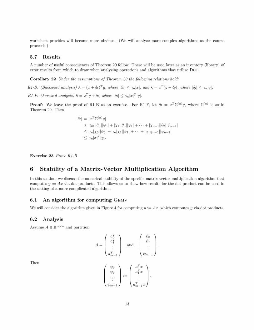
We will consider the algorithm given in Figure 4 for computing y := Ax, which computes y via dot products.

6.2 Analysis

Assume A ∈ Rm×n and partition

A =

aT0aT1...

aTm−1

and

ψ0

ψ1

...ψm−1

.

Then ψ0

ψ1

...ψm−1

:=

aT0 xaT1 x

...aTm−1x

.

13

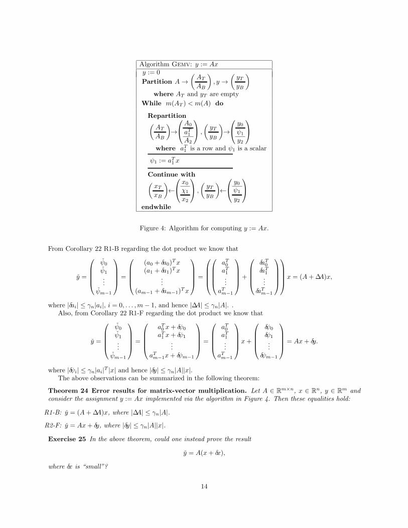
Algorithm Gemv: y := Axy := 0

Partition A→(ATAB

), y →

(yTyB

)where AT and yT are empty

While m(AT ) < m(A) do

Repartition(ATAB

)→

A0

aT1A2

,

(yTyB

)→

y0

ψ1

y2

where aT1 is a row and ψ1 is a scalar

ψ1 := aT1 x

Continue with(xTxB

)←

x0

χ1

x2

,

(yTyB

)←

y0

ψ1

y2

endwhile

Figure 4: Algorithm for computing y := Ax.

From Corollary 22 R1-B regarding the dot product we know that

y =

ψ0

ψ1

...

ψm−1

=

(a0 + δa0)Tx(a1 + δa1)Tx

...(am−1 + δam−1)Tx

=

aT0aT1...

aTm−1

+

δaT0δaT1

...δaTm−1

x = (A+ ∆A)x,

where |δai| ≤ γn|ai|, i = 0, . . . ,m− 1, and hence |∆A| ≤ γn|A|. .Also, from Corollary 22 R1-F regarding the dot product we know that

y =

ψ0

ψ1

...

ψm−1

=

aT0 x+ δψ0

aT1 x+ δψ1

...aTm−1x+ δψm−1

=

aT0aT1...

aTm−1

x+

δψ0

δψ1

...δψm−1

= Ax+ δy.

where |δψi| ≤ γn|ai|T |x| and hence |δy| ≤ γn|A||x|.The above observations can be summarized in the following theorem:

Theorem 24 Error results for matrix-vector multiplication. Let A ∈ Rm×n, x ∈ Rn, y ∈ Rm andconsider the assignment y := Ax implemented via the algorithm in Figure 4. Then these equalities hold:

R1-B: y = (A+ ∆A)x, where |∆A| ≤ γn|A|.

R2-F: y = Ax+ δy, where |δy| ≤ γn|A||x|.

Exercise 25 In the above theorem, could one instead prove the result

y = A(x+ δx),

where δx is “small”?

14

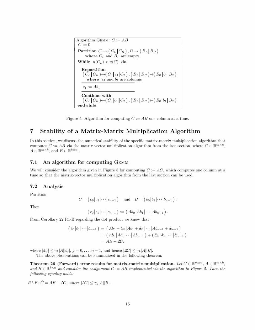
Algorithm Gemm: C := ABC := 0

Partition C →(CL CR

), B →

(BL BR

)where CL and BL are empty

While n(CL) < n(C) do

Repartition(CL CR

)→(C0 c1 C2

),(BL BR

)→(B0 b1 B2

)where c1 and b1 are columns

c1 := Ab1

Continue with(CL CR

)←(C0 c1 C2

),(BL BR

)←(B0 b1 B2

)endwhile

Figure 5: Algorithm for computing C := AB one column at a time.

7 Stability of a Matrix-Matrix Multiplication Algorithm

In this section, we discuss the numerical stability of the specific matrix-matrix multiplication algorithm thatcomputes C := AB via the matrix-vector multiplication algorithm from the last section, where C ∈ Rm×n,A ∈ Rm×k, and B ∈ Rk×n.

7.1 An algorithm for computing Gemm

We will consider the algorithm given in Figure 5 for computing C := AC, which computes one column at atime so that the matrix-vector multiplication algorithm from the last section can be used.

7.2 Analysis

PartitionC =

(c0 c1 · · · cn−1

)and B =

(b0 b1 · · · bn−1

).

Then (c0 c1 · · · cn−1

):=(Ab0 Ab1 · · · Abn−1

).

From Corollary 22 R1-B regarding the dot product we know that(c0 c1 · · · cn−1

)=(Ab0 + δc0 Ab1 + δc1 · · · Abn−1 + δcn−1

)=(Ab0 Ab1 · · · Abn−1

)+(δc0 δc1 · · · δcn−1

)= AB + ∆C.

where |δcj | ≤ γk|A||bj |, j = 0, . . . , n− 1, and hence |∆C| ≤ γk|A||B|.The above observations can be summarized in the following theorem:

Theorem 26 (Forward) error results for matrix-matrix multiplication. Let C ∈ Rm×n, A ∈ Rm×k,and B ∈ Rk×n and consider the assignment C := AB implemented via the algorithm in Figure 5. Then thefollowing equality holds:

R1-F: C = AB + ∆C, where |∆C| ≤ γk|A||B|.

15

Exercise 27 In the above theorem, could one instead prove the result

C = (A+ ∆A)(B + ∆B),

where ∆A and ∆B are “small”?

7.3 An application

A collaborator of ours recently implemented a matrix-matrix multiplication algorithm and wanted to checkif it gave the correct answer. To do so, he followed the following steps:

• He created random matrices A ∈ Rm×k, and C ∈ Rm×n, with positive entries in the range (0, 1).

• He computed C = AB with an implementation that was known to be “correct” and assumed it yieldsthe exact solution. (Of course, it has error in it as well. We discuss how he compensated for that,below.)

• He computed C = AB with his new implementation.

• He computed ∆C = C − C and checked that each of its entries satisfied δγi,j ≤ 2kuγi,j .

• In the above, he took advantage of the fact that A and B had positive entries so that |A||B| = AB = C.He also approximated γk = ku

1−ku with ku, and introduced the factor 2 to compensate for the fact thatC itself was inexactly computed.

References

[1] Paolo Bientinesi. Mechanical Derivation and Systematic Analysis of Correct Linear Algebra Algorithms.PhD thesis, Department of Computer Sciences, The University of Texas, 2006. Technical Report TR-06-46. September 2006.

[2] Paolo Bientinesi, John A. Gunnels, Margaret E. Myers, Enrique S. Quintana-Ortı, and Robert A. van deGeijn. The science of deriving dense linear algebra algorithms. ACM Transactions on MathematicalSoftware, 31(1):1–26, March 2005.

[3] Paolo Bientinesi and Robert A. van de Geijn. The science of deriving stability analyses. FLAME WorkingNote #33. Technical Report AICES-2008-2, Aachen Institute for Computational Engineering Sciences,RWTH Aachen, November 2008.

[4] Paolo Bientinesi and Robert A. van de Geijn. Goal-oriented and modular stability analysis. 32(1):286–308, 2011.

[5] John A. Gunnels, Fred G. Gustavson, Greg M. Henry, and Robert A. van de Geijn. FLAME: FormalLinear Algebra Methods Environment. ACM Trans. Math. Soft., 27(4):422–455, December 2001.

[6] Nicholas J. Higham. Accuracy and Stability of Numerical Algorithms. Society for Industrial and AppliedMathematics, Philadelphia, PA, USA, second edition, 2002.

16