Notes for EE 229A: Information and Coding Theory UC

Notes for EE 229A: Information and Coding Theory

UC Berkeley Fall 2020

Aditya Sengupta

January 17, 2021

Contents

Lecture 1: Introduction . . . . . . . . . . . . . . . . . . . . . . . . . . . . . . . . . . . . . . . . 4

1.1 Entropy . . . . . . . . . . . . . . . . . . . . . . . . . . . . . . . . . . . . . . . . . . . . . . . 5

Lecture 2: Entropy and mutual information, relative entropy . . . . . . . . . . . . . . . . 7

2.1 Entropy . . . . . . . . . . . . . . . . . . . . . . . . . . . . . . . . . . . . . . . . . . . . . . . 7

2.2 Joint Entropy . . . . . . . . . . . . . . . . . . . . . . . . . . . . . . . . . . . . . . . . . . . . 8

2.3 Conditional entropy . . . . . . . . . . . . . . . . . . . . . . . . . . . . . . . . . . . . . . . . 8

2.4 Mutual information . . . . . . . . . . . . . . . . . . . . . . . . . . . . . . . . . . . . . . . . . 9

2.5 Jensen’s inequality . . . . . . . . . . . . . . . . . . . . . . . . . . . . . . . . . . . . . . . . . 9

Lecture 3: Mutual information and relative entropy . . . . . . . . . . . . . . . . . . . . . . 12

3.1 Mutual information . . . . . . . . . . . . . . . . . . . . . . . . . . . . . . . . . . . . . . . . . 12

3.2 Chain rule for mutual information (M.I.) . . . . . . . . . . . . . . . . . . . . . . . . . . . . . 12

3.3 Relative entropy . . . . . . . . . . . . . . . . . . . . . . . . . . . . . . . . . . . . . . . . . . 13

Lecture 4: Mutual information and binary channels . . . . . . . . . . . . . . . . . . . . . . 15

4.1 Binary erasure channel example . . . . . . . . . . . . . . . . . . . . . . . . . . . . . . . . . . 15

4.2 The uniform distribution maximizes entropy . . . . . . . . . . . . . . . . . . . . . . . . . . . 16

4.3 Properties from C-T 2.7 . . . . . . . . . . . . . . . . . . . . . . . . . . . . . . . . . . . . . . 16

Lecture 5: Data processing inequality, asymptotic equipartition . . . . . . . . . . . . . . 18

5.1 Data Processing Inequality . . . . . . . . . . . . . . . . . . . . . . . . . . . . . . . . . . . . . 18

5.2 AEP: Entropy and Data Compression . . . . . . . . . . . . . . . . . . . . . . . . . . . . . . 19

5.3 Data Compression . . . . . . . . . . . . . . . . . . . . . . . . . . . . . . . . . . . . . . . . . 21

Lecture 6: AEP, coding . . . . . . . . . . . . . . . . . . . . . . . . . . . . . . . . . . . . . . . . 22

1

6.1 Markov sequences . . . . . . . . . . . . . . . . . . . . . . . . . . . . . . . . . . . . . . . . . . 22

6.2 Codes . . . . . . . . . . . . . . . . . . . . . . . . . . . . . . . . . . . . . . . . . . . . . . . . 23

6.3 Uniquely decodable and prefix codes . . . . . . . . . . . . . . . . . . . . . . . . . . . . . . . 24

Lecture 7: Designing Optimal Codes, Kraft’s Inequality . . . . . . . . . . . . . . . . . . . 25

7.1 Prefix codes . . . . . . . . . . . . . . . . . . . . . . . . . . . . . . . . . . . . . . . . . . . . . 25

7.2 Optimal Compression . . . . . . . . . . . . . . . . . . . . . . . . . . . . . . . . . . . . . . . 27

7.3 Kraft’s Inequality . . . . . . . . . . . . . . . . . . . . . . . . . . . . . . . . . . . . . . . . . . 27

7.4 Coding Schemes and Relative Entropy . . . . . . . . . . . . . . . . . . . . . . . . . . . . . . 29

7.5 The price for assuming the wrong distribution . . . . . . . . . . . . . . . . . . . . . . . . . . 32

Lecture 8: Prefix code generality, Huffman codes . . . . . . . . . . . . . . . . . . . . . . . . 33

8.1 Huffman codes . . . . . . . . . . . . . . . . . . . . . . . . . . . . . . . . . . . . . . . . . . . 34

8.2 Limitations of Huffman codes . . . . . . . . . . . . . . . . . . . . . . . . . . . . . . . . . . . 35

Lecture 9: Arithmetic coding . . . . . . . . . . . . . . . . . . . . . . . . . . . . . . . . . . . . . 36

9.1 Overview and Setup, Infinite Precision . . . . . . . . . . . . . . . . . . . . . . . . . . . . . . 36

9.2 Finite Precision . . . . . . . . . . . . . . . . . . . . . . . . . . . . . . . . . . . . . . . . . . . 37

9.3 Invertibility . . . . . . . . . . . . . . . . . . . . . . . . . . . . . . . . . . . . . . . . . . . . . 37

Lecture 10: Arithmetic coding wrapup, channel coding . . . . . . . . . . . . . . . . . . . . 38

10.1 Communication over noisy channels . . . . . . . . . . . . . . . . . . . . . . . . . . . . . . . . 38

Lecture 11: Channel coding efficiency . . . . . . . . . . . . . . . . . . . . . . . . . . . . . . . 40

11.1 Noisy typewriter channel . . . . . . . . . . . . . . . . . . . . . . . . . . . . . . . . . . . . . . 40

Lecture 12: Rate Achievability . . . . . . . . . . . . . . . . . . . . . . . . . . . . . . . . . . . . 42

Lecture 13: Joint Typicality . . . . . . . . . . . . . . . . . . . . . . . . . . . . . . . . . . . . . 44

13.1 BSC Joint Typicality Analysis . . . . . . . . . . . . . . . . . . . . . . . . . . . . . . . . . . . 44

Lecture 14: Fano’s Inequality for Channels . . . . . . . . . . . . . . . . . . . . . . . . . . . . 47

Lecture 15: Polar Codes, Fano’s Inequality . . . . . . . . . . . . . . . . . . . . . . . . . . . . 48

15.1 Recap of Rate Achievability . . . . . . . . . . . . . . . . . . . . . . . . . . . . . . . . . . . . 48

15.2 Source Channel Theorem . . . . . . . . . . . . . . . . . . . . . . . . . . . . . . . . . . . . . 48

15.3 Polar Codes . . . . . . . . . . . . . . . . . . . . . . . . . . . . . . . . . . . . . . . . . . . . . 49

Lecture 16: Polar Codes . . . . . . . . . . . . . . . . . . . . . . . . . . . . . . . . . . . . . . . . 51

Lecture 17: Information Measures for Continuous RVs . . . . . . . . . . . . . . . . . . . . 53

17.1 Differential Entropy . . . . . . . . . . . . . . . . . . . . . . . . . . . . . . . . . . . . . . . . 54

17.2 Differential entropy of popular distributions . . . . . . . . . . . . . . . . . . . . . . . . . . . 55

2

17.3 Properties of differential entropy . . . . . . . . . . . . . . . . . . . . . . . . . . . . . . . . . 57

Lecture 18: Distributed Source Coding, Continuous RVs . . . . . . . . . . . . . . . . . . . 58

18.1 Distributed Source Coding . . . . . . . . . . . . . . . . . . . . . . . . . . . . . . . . . . . . . 58

18.2 Differential Entropy Properties . . . . . . . . . . . . . . . . . . . . . . . . . . . . . . . . . . 59

18.3 Entropy Maximization . . . . . . . . . . . . . . . . . . . . . . . . . . . . . . . . . . . . . . . 60

18.4 Gaussian Channel Capacity Formulation . . . . . . . . . . . . . . . . . . . . . . . . . . . . . 62

Lecture 20: Maximum Entropy Principle, Supervised Learning . . . . . . . . . . . . . . . 64

20.1 The principle of maximum entropy . . . . . . . . . . . . . . . . . . . . . . . . . . . . . . . . 64

20.2 Supervised Learning . . . . . . . . . . . . . . . . . . . . . . . . . . . . . . . . . . . . . . . . 65

3

Lecture 1: Introduction 4

EE 229A: Information and Coding Theory Fall 2020

Lecture 1: IntroductionLecturer: Kannan Ramchandran 27 August Aditya Sengupta

Note: LATEX format adapted from template for lecture notes from CS 267, Applications of Parallel Comput-ing, UC Berkeley EECS department.

Information theory answers two fundamental questions.

1. What are the fundamental limits of data compression? The answer is the entropy of the sourcedistribution.

2. What are the fundamental limits of reliable communication? The answer is the channel capacity.

Information theory has its roots in communications, but now has influence in statistical physics, theoreticalcomputer science, statistical inference and theoretical statistics, portfolio theory, and measure theory.

Historically, 18th and 19th century communication systems were not seen as a unified field of study/engi-neering. Claude Shannon saw that they were all connected, and said: Every communication system has theform f1(t) → [T ] → F (t) → [R] → f2(t). He made some assumptions that don’t hold today; for one thing,he assumed a noiseless channel, and analog signals.

There’s a movie about Shannon! The Bit Player.

Shannon called his work “A Mathematical Theory of Communication” - others then called it Shannon’stheory of communication. The key insight: no matter what you’re using to send and receive messages, youcan use the common currency of bits to encode messages.

Figure 1.1: Shannon’s channel diagram

Shannon introduced three new concepts:

Lecture 1: Introduction 5

1. The entropy, as above

2. not sure

3. not sure

The separation theorem states that source and channel coders do their jobs optimally and separately foroptimal end-to-end performance.

After 70+ years, all communication systems are built on the principles of information theory, and it providestheoretical benchmarks for engineering systems.

1.1 Entropy

In information theory, entropy is a measure of the information content contained in any message or flow ofinformation.

Example 1.1. Take a source S = {A,B,C,D} with P(x) = 14 for each x ∈ S. A uniform source

might produce a sequence like ADCABCBA . . . , assuming these are iid. How manybinary questions would you expect to ask to figure out what each symbol is?

We expect to ask 2 questions, and because we’ve done 126 we know this is because

H(x) = −∑X

P(X) log2 P(X) = −4 · 1

4log2

1

4= −1 · (−2) = 2 (1.1)

and more concretely, you can ask the Huffman tree of questions:

• Is X ∈ {AB}?

• If yes, is X = A?

– If yes, X = A.

– If no, X = B.

• If no, is X = C?

– If yes, X = C.

– If no, X = D.

�

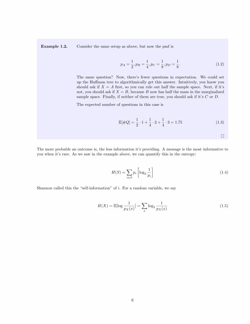
Example 1.2. Consider the same setup as above, but now the pmf is

pA =1

2, pB =

1

4, pC =

1

8, pD =

1

8. (1.2)

The same question? Now, there’s fewer questions in expectation. We could setup the Huffman tree to algorithmically get this answer. Intuitively, you know youshould ask if X = A first, so you can rule out half the sample space. Next, if it’snot, you should ask if X = B, because B now has half the mass in the marginalizedsample space. Finally, if neither of them are true, you should ask if it’s C or D.

The expected number of questions in this case is

E[#Q] =1

2· 1 +

1

4· 2 +

1

4· 3 = 1.75 (1.3)

�

The more probable an outcome is, the less information it’s providing. A message is the most informative toyou when it’s rare. As we saw in the example above, we can quantify this in the entropy:

H(S) =∑i∈S

pi

[log2

1

pi

](1.4)

Shannon called this the “self-information” of i. For a random variable, we say

H(X) = E[log1

pX(x)] =

∑x

log2

1

pX(x)(1.5)

6

Lecture 2: Entropy and mutual information, relative entropy 7


Lecture 2: Entropy and mutual information, relative entropyLecturer: Kannan Ramchandran 1 September Aditya Sengupta

2.1 Entropy

Previously, we saw that the entropy of a discrete RV X was given by

H(X) = E[log1

pX(x)] =

∑x

log2

1

pX(x)(2.1)

We say that the entropy is label-invariant, as it depends only on the distribution and not on the specificvalues that the variable could take on. This contrasts properties like expectation and variance, which dodepend on the values the variable could take on.

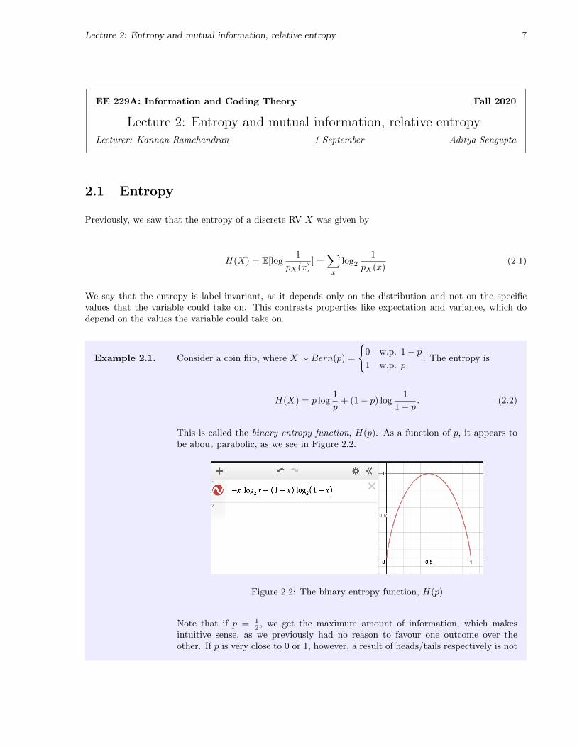
Example 2.1. Consider a coin flip, where X ∼ Bern(p) =

{0 w.p. 1− p1 w.p. p

. The entropy is

H(X) = p log1

p+ (1− p) log

1

1− p. (2.2)

This is called the binary entropy function, H(p). As a function of p, it appears tobe about parabolic, as we see in Figure 2.2.

Figure 2.2: The binary entropy function, H(p)

Note that if p = 12 , we get the maximum amount of information, which makes

intuitive sense, as we previously had no reason to favour one outcome over theother. If p is very close to 0 or 1, however, a result of heads/tails respectively is not


very surprising, and so its entropy is less.�

2.2 Joint Entropy

If we have two RVs, say X1 and X2, then their joint entropy follows directly from their joint distribution:

H(X1, X2) = E[log2

1

p(X1, X2)

]. (2.3)

If X1 and X2 are independent, then p(X1, X2) = p(X1)p(X2); the distribution splits, and therefore so doesthe entropy:

H(X1, X2) = E[log2

1

p(X1, X2)

]= E

[log2

1

p(X1)

]+ E

[log2

1

p(X2)

](2.4)

Therefore, X |= Y =⇒ H(X,Y ) = H(X) +H(Y ).

We see that the log in the definition of entropy ensures that entropy is additive: the entropy of independentRVs is the sum of the individual entropies.

2.3 Conditional entropy

The more general law based on conditioning is

H(X,Y ) = H(X) +H(Y |X), (2.5)

where

H(Y |X) = E[log

1

p(y|x)

]=∑x

∑y

p(x, y) log1

p(y|x). (2.6)

H(Y |X) is referred to as the conditional entropy of Y given X.

We can extend this to more than two variables, if we just look at the definition above with two variables ata time:

H(X,Y, Z) = H(X) +H(Y,Z|X) = H(X) +H(Y |X) +H(Z|Y,X). (2.7)

This is the chain rule of entropy.


Let’s break down the expression H(Y |X) a bit more.

H(Y |X) =∑x

∑y

p(x, y) log1

p(x, y)

=∑x

p(x)∑y

p(y|x) log1

p(y|x)

=∑x

p(x)H(Y | X = x).

(2.8)

And the extension to the three-variable setting:

H(Y, Z|X) =∑x

p(x)H(Y,Z|X = x)

=∑x

p(x)H(Y |X = x) +∑x

p(x)H(Z|Y,X = x)

= H(Y |X) +H(Z|Y,X).

(2.9)

This is just like H(Y,Z) = H(Y ) +H(Z|Y ), but conditioning everything on X.

2.4 Mutual information

The mutual information of two RVs, I(X;Y ), is given by

I(X;Y ) = H(X)−H(X|Y ). (2.10)

We interpret this as “how much information does Y convey about X?”

The mutual information can be shown to be symmetric, i.e. X gives as much information about Y as Ygives about X.

I(X;Y ) = I(Y ;X) (2.11)

H(X)−H(X|Y ) = H(Y )−H(Y |X). (2.12)

2.5 Jensen’s inequality

Definition 2.1. A real-valued function f is convex on an interval [a, b] if for any x1, x2 ∈ [a, b] and any λsuch that 0 < λ < 1,

f(λx1 + (1− λ)x2) ≤ λf(x1) + (1− λ)f(x2)


A couple useful properties:

• If f is doubly differentiable, then f ′′(x) ≥ 0 ⇐⇒ f is convex.

• If −f is convex then f is concave.

Theorem 2.1 (Jensen’s Inequality for Probabilities). For any random variable X and any convex functionf ,

f(E[X]) ≤ E[f(X)].

Proof. Let t(x) be the tangent line of f(x) at some point c. We can say

f(x) ≥ f(c) + f ′(c)(x− c), (2.13)

i.e. f(x) is above the tangent line.

Take c = E[X]; then we have

f(x) ≥ f(E[X]) + f ′(E[X])(X − E[X]) (2.14)

E[f(X)] ≥ f(E[X]) + f ′(E[X]) · 0 (2.15)

E[f(X)] ≥ f(E[X]). (2.16)

A quick example of this is: f(x) = x2. Jensen’s tells us that E[X2] ≥ E[X]2, i.e. E[X2] − E[X]2 ≥ 0. Thismakes sense if we think of this expression as var(X).

If we consider f(x) = − log x, we get

logE[X] ≥ E[logX]. (2.17)

From this, we can get a couple of useful properties of entropy: by definition, we know that H(X) ≥ 0, andwe can show using Equation 2.17 that entropy is upper-bounded by the size of the alphabet:

H(X) = E[log p(x)] ≤ logE[p(x)] = log |X | (2.18)

More properties of mutual information:

1. I(X;Y ) = I(Y ;X)

2. I(X;Y ) ≥ 0 ∀X,Y

3. I(X;Y ) = 0 ⇐⇒ X |= Y .

Figure 2.3: Mutual information diagrams

11

Lecture 3: Mutual information and relative entropy 12


Lecture 3: Mutual information and relative entropyLecturer: Kannan Ramchandran 3 September Aditya Sengupta

3.1 Mutual information

We’ll start with a closed form for mutual information in terms of a probability distribution.

I(X;Y ) = H(X)−H(X|Y ) (3.1)

=∑x

p(x) log1

p(x)−∑x

∑y

p(x, y) log1

p(x|y)(3.2)

=∑x

∑y

p(x, y) log1

p(x)−∑x

∑y

p(x, y) log1

p(x|y)(3.3)

=∑x

∑y

p(x, y) logp(x|y)

p(x). (3.4)

We can use this to show that mutual information is symmetric:

p(x|y)

p(x)=

p(x, y)

p(x)p(y)=p(y|x)

p(y)(3.5)

I(X;Y ) =∑x

∑y

p(x, y) logp(x, y)

p(x)p(y)(3.6)

=∑x

∑y

p(x, y) log1

p(x)p(y)−∑x

∑y

p(x, y) log1

p(x, y)(3.7)

= H(X) +H(Y )−H(X,Y ). (3.8)

Mutual information must be nonnegative, and I(X;Y ) = 0 ⇐⇒ X |= Y . From this, we get that H(X,Y ) =H(X) +H(Y ) if and only if X |= Y .

3.2 Chain rule for mutual information (M.I.)

Suppose we have three RVs, X,Y1, Y2. Consider I(X;Y1, Y2), which we can interpret as the amount ofinformation that (Y1, Y2) give us about X. We can split this up similarly to how we would for entropy:

I(X;Y1, Y2) = I(X;Y1) + I(X;Y2|Y1) (3.9)

Lecture 3: Mutual information and relative entropy 13

3.3 Relative entropy

Relative entropy is also known as Kullback-Leibler (K-L) divergence.

Definition 3.1. The relative entropy between two distributions p, q is

D(p ‖ q) =∑x∈X

p(x) logp(x)

q(x), (3.10)

or alternatively,

D(p ‖ q) = Ex∼p[log

p(x)

q(x)

]. (3.11)

Relative entropy has the following properties:

1. In general, D(p ‖ q) 6= D(q ‖ p) :(

2. D(p ‖ p) = 0

3. D(p ‖ q) ≥ 0 for all distributions p, q, with equality iff p = q.

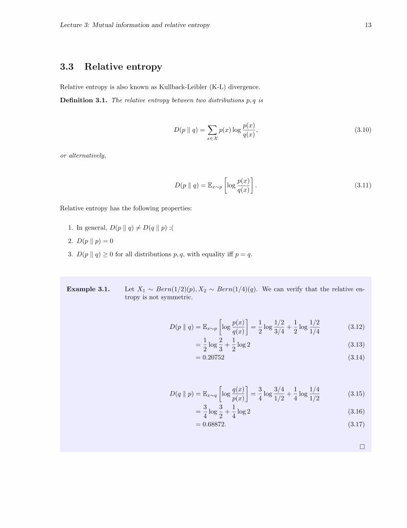
Example 3.1. Let X1 ∼ Bern(1/2)(p), X2 ∼ Bern(1/4)(q). We can verify that the relative en-tropy is not symmetric.

D(p ‖ q) = Ex∼p[log

p(x)

q(x)

]=

1

2log

1/2

3/4+

1

2log

1/2

1/4(3.12)

=1

2log

2

3+

1

2log 2 (3.13)

= 0.20752 (3.14)

D(q ‖ p) = Ex∼q[log

q(x)

p(x)

]=

3

4log

3/4

1/2+

1

4log

1/4

1/2(3.15)

=3

4log

3

2+

1

4log 2 (3.16)

= 0.68872. (3.17)

�

I(X;Y ) can be expressed in terms of the relative entropy between their joint distribution and the productof their marginals.

I(X;Y ) =∑x,y

p(x, y) logp(x, y)

p(x)p(y)(3.18)

= D(p(x, y) ‖ p(x) · p(y)). (3.19)

Theorem 3.1. Let p(x), q(x), x ∈ X be two PMFs. Then D(p ‖ q) ≥ 0, with equality iff p(x) = q(x) ∀x ∈ X .

Proof. Let A = {x | p(x) > 0} be the support set of p(x).

From the definition,

−D(p ‖ q) = −∑x∈A

p(x) logp(x)

q(x)(3.20)

=∑x∈A

p(x) logq(x)

p(x)= Ex∼p

[log

q(x)

p(x)

](3.21)

Using Jensen’s inequality,

−D(p ‖ q) ≤ log∑x∈A

p(x)q(x)

p(x)= log

∑x∈A

q(x). (3.22)

Since q and p may not have exactly the same support,∑x∈A q(x) ≤ 1 and so

−D(p ‖ q) ≤ log 1 = 0 (3.23)

D(p ‖ q) ≥ 0. (3.24)

Remark 3.2. Since log t is concave in t, we have equality in 3.22 iff q(x)p(x) = c everywhere, i.e. q(x) =

cp(x) ∀x ∈ A. Due to normalization, this can only occur when c = 1, i.e. they are identical inside thesupport. Further, we have equality in 3.23 iff the support of both PMFs is the same. Putting those together,the distributions must be exactly the same. Therefore, D(p ‖ q) = 0 ⇐⇒ p(x) = q(x) ∀x ∈ X .

Corollary 3.3. 1. I(X;Y ) = D(p(x, y) ‖ p(x) · p(y)) ≥ 0

2. H(X|Y ) ≤ H(X). Conditioning reduces entropy.

We can interpret this as saying that on average, the uncertainty of X after we observe Y is no more thanthe uncertainty of X unconditionally. “More knowledge cannot hurt”.

Among all possible distributions over a finite alphabet, the uniform distribution achieves the maximumentropy.

14

Lecture 4: Mutual information and binary channels 15


Lecture 4: Mutual information and binary channelsLecturer: Kannan Ramchandran 8 September Aditya Sengupta

4.1 Binary erasure channel example

Example 4.1. Consider the binary erasure channel where X ∈ {0, 1} and Y ∈ {0, 1, ∗}, Let Y = Xwith probability 1

2 and Y = ∗ with probability 12 , individually for either case of X.

(todo if I care, BEC diagram). Suppose X ∼ Bern(1/2), so that

Y =

0 w.p. 1

4

∗ w.p. 12

1 w.p. 14

(4.1)

H(X) = H2

(1

2,

1

2

)(4.2)

H(Y ) = H3

(1

4,

1

2,

1

4

)= 1.5 (4.3)

We can find the conditional entropies, using the fact that X is symmetric:

H(Y |X) = H(Y |X = 0) = H2

(1

2,

1

2

)= 1 (4.4)

H(X|Y = y) =

{0 y ∈ {0, 1}1 y = ∗

(4.5)

H(X|Y ) = E[H(X|Y = y)] = 0.5 (4.6)

Therefore, the mutual information either way is

H(X)−H(X|Y ) = 1− 0.5 = 0.5 (4.7)

H(Y )−H(Y |X) = 1.5− 1 = 0.5 (4.8)

�

Lecture 4: Mutual information and binary channels 16

4.2 The uniform distribution maximizes entropy

Theorem 4.1. Let an RV X be defined on X with |X | = n. Let U be the uniform distribution on X . ThenH(X) ≤ H(U).

Proof.

H(U)−H(X) =∑X

1

nlog n+

∑x

p(x) log p(x) (4.9)

=∑x

p(x)(log n) +∑x

p(x) log p(x) (4.10)

=∑x

p(x) log

(p(x)

1/n

)(4.11)

= D(p ‖ U) ≥ 0. (4.12)

4.3 Properties from C-T 2.7

Theorem 4.2 (Log-Sum Inequality). For nonnegative numbers (ai)ni=1 and (bi)

ni=1,

n∑i=1

ai logaibi≥

(n∑i=1

ai

)log

∑ni=1 ai∑ni=1 bi

, (4.13)

with equality if and only if aibi

= const.

Proof. (Almost directly from C&T 2.7.1)

f(t) = t log t is convex on positive inputs, and therefore Jensen’s inequality applies; let {αi} be a partitionof unity, then

∑i

αif(ti) ≥ f

(∑i

αiti

), (4.14)

for any {ti} such that all elements are positive. In particular, this works for αi = bi∑j bj

and ti = aibi

;

substituting this into Jensen’s gives us

∑ ai∑bj

logaibi≥∑ ai∑

bjlog∑ ai∑

bj. (4.15)

Theorem 4.3 (Convexity of Relative Entropy). D(p ‖ q) is convex in (p, q), i.e. if (p1, q1), (p2, q2) are twopairs of distribution, then

D(λp1 + (1− λ)p2 ‖ λq1 + (1− λ)q2) ≤ λD(p1 ‖ q1) + (1− λ)D(p2 ‖ q2) (4.16)

Theorem 4.4 (Concavity of entropy). H(p) is concave in p.

Proof.

H(p) = log |X | −D(p ‖ U) (4.17)

Since relative entropy is convex in p, its negative must be concave (and this is not affected by the constantoffset.)

17

Lecture 5: Data processing inequality, asymptotic equipartition 18


Lecture 5: Data processing inequality, asymptotic equipartitionLecturer: Kannan Ramchandran 10 September Aditya Sengupta

5.1 Data Processing Inequality

The data processing inequality states that if X → Y → Z is a Markov chain, then p(Z|Y,X) = p(Z|Y ) andso

I(X;Y ) ≥ I(X;Z) (5.1)

I(Y ;Z) ≥ I(X;Z). (5.2)

More rigorously,

I(X;Y,Z) = I(X;Y ) + I(X;Z|Y ) = I(X;Y )

= I(X;Z) + I(X;Y |Z)(5.3)

I(X,Y ;Z) = I(X;Z) + I(Y ;Z|X) = I(X;Z)

= I(Y ;Z) + I(X;Z|Y )(5.4)

Corollary 5.1. If Z = g(Y ), we have I(X;Y ) ≥ I(X; g(Y )).

Proof. X → Y → g(Y ) forms a Markov chain.

Corollary 5.2. If X → Y → Z then I(X;Y Z) ≤ I(X;Y |Z).

Proof.

I(X;Y Z) = I(X;Y ) + I(X;Z|Y )

I(X;Z) + I(X;Y |Z)(5.5)

If X − Y − Z forms a Markov chain, then the dependency between X and Y is decreased by observation ofa “downstream” RV Z.

How crucial is the Markov chain assumption? If X − Y − Z do not form a chain, then it’s possible forI(X;Y |Z) > I(X,Y ).


Example 5.1. LetX,Y ∼ Bern(1/2) and I(X;Y ) = 0. Let Z = X⊕Y . Therefore Z = 1{X 6= Y }.

Consider

I(X;Y |Z) = H(X|Z)−H(X|Y,Z) = H(X) = 1− 0 = 1 (5.6)

and I(X;Y ) = 0. These do not form a chain but still satisfy the property.�

5.2 AEP: Entropy and Data Compression

Entropy is directly related to the fundamental limits of data compression.

1. For a sequence of n i.i.d. RVs, Xi ∼ Bern(1/2), we need nH(X1) = n bits.

2. If Xii.i.d.∼ Bern(0.11), we need nH(X1) = nH2(0.11) = n

2 bits.

For a rough analysis of the entropy of a sequence, consider (Xi)ni=1 ∼ Bern(p). The probability of a particular

sequence drawn from this distribution having k ones and n− k zeros is

p(X1, . . . , Xn) = pk(1− p)n−k (5.7)

= 2k log p+(n−k) log(1−p) (5.8)

= 2−n( kn log p+ n−k

n log(1−p)) (5.9)

By the law of large numbers, k ' np, so we can more simply write

p(X1, . . . , Xn) = 2−n(p log 1p−(1−p) log 1

1−p ) (5.10)

= 2−nH2(p). (5.11)

These are typical sequences with the same probability of occurring. Although there are 2n possible sequences,the “typical” ones will have probability 2−nH(X). The number of typical sequences is

(n

np

)=

n!

(np)!(n− np)!(5.12)

and by Stirling’s approximation we get (setting p = 1− p):


(n

np

)≈ (n/e)n

(np/e)np(np/e)np(5.13)

= p−npp−np (5.14)

= 2n(p log 1p +p log 1

p ) = 2nH2(p) (5.15)

If n = 1000, p = 0.11, then H(X) = 12 . The number of possible sequences is 21000, but there are only about

2500 typical sequences.

The ratio of typical sequences to the total number of sequences is

2nH(X)

2n= 2n(H(X)−1) n→∞−→ 0, (5.16)

for H(X) 6= 1.

Lemma 5.3 (WLLN for entropy). Let (Xi)ni=1

i.i.d.∼ p. Then by the weak law of large numbers,

− 1

nlog p(X1, . . . , Xn)

p−→ H(X) (5.17)

Proof. RVs p(Xi) are i.i.d., and so by

− 1

nlog p(X1, . . . , Xn) = − 1

n

n∑i=1

log p(Xi)p−→ −E[log p(X)] = H(X). (5.18)

The AEP enables us to partition the sequence (Xi)ni=1 ∼ p into a typical set, containing sequences with

probability approximately 2−nH(X) (with leeway of ε), and an atypical set, containing the rest. This willallow us to compress any sequence in the typical set to n(H(X) + ε) bits.

Definition 5.1. A typical set A(n)ε with respect to a distribution p is the set of sequences (x1, . . . , xn) ∈ Xn

with probability

2−n(H(X)+ε) ≤ p(x1, . . . , xn) ≤ 2−n(H(X)−ε). (5.19)

Example 5.2. Suppose in our Bern(0.11) sequence, with n = 1000, we let ε = 0.01. Then thetypical set is

{(X1, . . . , Xn) | 2−510 ≤ p(X1, . . . , Xn) ≤ 2−490} (5.20)

�

Some properties of the typical set are as follows:

1. For a sequence of RVs (Xi)ni=1

i.i.d.∼ p and sufficiently large n,

P((Xi) ∈ A(n)ε ) ≥ 1− ε (5.21)

2. (1− ε)2n(H(X1)−ε ≤ |A(n)ε | ≤ 2n(H(X1)+ε

5.3 Data Compression

Theorem 5.4. Let {Xi}ni=1i.i.d.∼ Bern(p) and ε > 0. Then there exists an invertible mapping of (X1, . . . , Xn)

into binary codewords of length l(X1, . . . , Xn) where

E[l(X1, . . . , Xn)] ≤ n[H(X) + 2ε]. (5.22)

Proof. Consider our scheme which encodes A(n)ε using codewords of length n(H(X) + ε), and the atypical

set using codewords of length n. Averaging over those two and using property 1 above, the expected valueof a sequence length does not exceed the typical set values by more than ε.

21

Lecture 6: AEP, coding 22


Lecture 6: AEP, codingLecturer: Kannan Ramchandran 15 September Aditya Sengupta

Previously, we saw that exploiting the AEP for compression gave us an expected value of compressed lengthslightly greater than nH(X):

E[l(Xi)] = n(H(X) + ε)P(A(n)ε ) + n(1− P(A(n)

ε )) ≈ n(H(X) + 2ε) (6.1)

With more careful counting, the code length of a typical sequence is n(H(X) + ε) + 1.

6.1 Markov sequences

Shannon considered the problem of modeling and compressing English text. To do this, we’ll need tointroduce the concept of entropy rate.

Definition 6.1. For a sequence of RVs X1, . . . , Xn, where the sequence is not necessarily i.i.d., the entropyrate of the sequence is

H(X) = limn→∞

1

nH(X1, . . . , Xn), (6.2)

if the limit exists.

For instance, if the sequence is i.i.d., H(X) = H(X1). In some (contrived) cases, H(X) is not well-defined;see C&T p75.

We can find the entropy rate of a stationary Markov chain:

H(X1, . . . , Xn) = H(X1) +

n−1∑i=1

H(Xi+1|Xi) (6.3)

= H(X1) + (n− 1)H(X2|X1) (6.4)

As n→∞, the entropy rate just becomes H(X2|X1).

Example 6.1. Consider the following Markov chain.

0 11− αα

β1− β

Lecture 6: AEP, coding 23

For example, we can take α = β = 0.11. Then, our entropy rate tends to

H(X2|X1) = H(X2|X1 = 0)P(X1 = 0) +H(X2|X1 = 1)P(X1 = 1). (6.5)

We can find that the stationary distribution in general is[

βα+β ,

αα+β

], so that lets

us plug into the conditional entropy:

H(X2|X1) = H2(0.11) · 1

2+H2(0.89) · 1

2= 0.5 (6.6)

Therefore, we can compress the Markov chain of length 1000 to about 500 bits.�

6.2 Codes

Previously, we used the AEP to obtain coding schemes that asymptotically need H(X1) bits per symbol to

compress the source X1, . . . , Xni.i.d.∼ p.

Now, we turn our attention to “optimal” coding schemes that compress X1, . . . , Xni.i.d.∼ p for finite values

of n.

Definition 6.2. A code C : X → {0, 1}l is an injective function that maps letters of X to binary codewords.

We denote by C(x) the code for x, and we denote by l(x) the length of the code, for x ∈ X .

Definition 6.3. The expected length L of a code C is defined as

L∆=∑x∈X

l(x)p(x). (6.7)

We want our codes to be uniquely decodable, i.e. any x can only have one representation in code. Specifically,we will focus on a class of codes called prefix codes, which have nice mathematical properties.

Our task is to devise a coding scheme C from a class of uniquely decodable prefix codes such that L isminimized.

Example 6.2. Let X = {a, b, c, d} and let pX = { 12 ,

14 ,

18 ,

18}. We want a binary code, D = {0, 1}.

If we Huffman encode, this turns out to be

c(a) = 0, c(b) = 10, c(c) = 110, c(d) = 111 (6.8)

l(a) = 1, l(b) = 2, l(c) = 3, l(d) = 3. (6.9)

We see that in this case, L = H(p): we’ve achieved the optimal average length(although we haven’t shown it’s optimal yet).

�

The optimal length is not always the entropy of the distribution, due to “discretization” effects.

Example 6.3. Let X = {a, b, c} and pX = { 13 ,

13 ,

13}. The Huffman code might be a → 0, b →

10, c → 11 or equivalent. L = 1+2+23 = 1.66, and H(X) = log2 3 = 1.58. Here the

entropy cannot be reached.�

6.3 Uniquely decodable and prefix codes

Suppose we have a code that has a → 0, d → 0. This is a singular code at the symbol level, because if weget a 0 we do not know whether to decode it to a or d.

Suppose we have a code a→ 0, b→ 010, c→ 01, d→ 10. If we get the code 010, we do not know whether todecode it to b, ca, or ad. This is a singular code in extension space.

A code is called uniquely decodable if its extension is non-singular. A code is called a prefix code if nocodeword is a prefix of any other.

24

Lecture 7: Designing Optimal Codes, Kraft’s Inequality 25


Lecture 7: Designing Optimal Codes, Kraft’s InequalityLecturer: Kannan Ramchandran 17 September Aditya Sengupta

Our goal with coding theory is to find the function C to minimize the average message length L. Codesmust also have certain constraints placed on them: they must be uniquely decodable, and we will focus onprefix codes.

Definition 7.1. A code is called uniquely decodable (UD) if its extension C∗ is nonsingular.

A code is UD if no two source symbol sequences correspond to the same encoded bitstream.

Definition 7.2. A code is called a prefix code or instantaneous code if no codeword is the prefix of any other.

prefix codes ⊂ uniquely decodable codes ⊂ codes

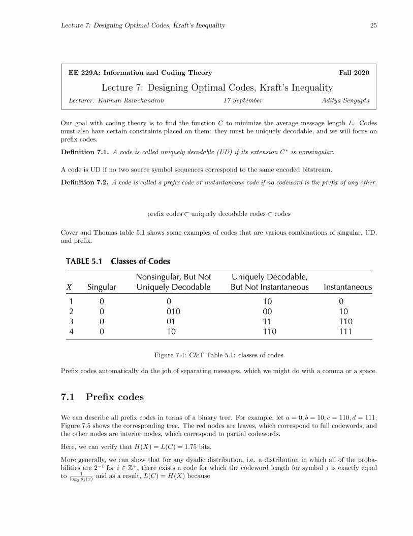
Cover and Thomas table 5.1 shows some examples of codes that are various combinations of singular, UD,and prefix.

Figure 7.4: C&T Table 5.1: classes of codes

Prefix codes automatically do the job of separating messages, which we might do with a comma or a space.

7.1 Prefix codes

We can describe all prefix codes in terms of a binary tree. For example, let a = 0, b = 10, c = 110, d = 111;Figure 7.5 shows the corresponding tree. The red nodes are leaves, which correspond to full codewords, andthe other nodes are interior nodes, which correspond to partial codewords.

Here, we can verify that H(X) = L(C) = 1.75 bits.

More generally, we can show that for any dyadic distribution, i.e. a distribution in which all of the proba-bilities are 2−i for i ∈ Z+, there exists a code for which the codeword length for symbol j is exactly equalto 1

log2 pj(x) and as a result, L(C) = H(X) because


Figure 7.5: A tree corresponding to a prefix code


L(C) = E[lj(x)] =∑j

pj(x) log2

1

log2 pj(x)= H(X). (7.1)

For distributions that are not dyadic, there is a gap; for example, the optimal code for the distribution[13 ,

13 ,

13

]has L(C) = 1.66 bits whereas H(X) = 1.58 bits.

7.2 Optimal Compression

Seeing that L(C) = H(X) in nice cases and L(C) > H(X) in some other cases, we are motivated to ask thefollowing questions:

1. Are there codes that can achieve compression rates lower than H?

2. If not, what is the best achievable compression rate compared to H?

We can set this up as an optimization problem: let X ∼ p be defined over an alphabet X = {1, 2, . . . ,m}.Without loss of generality, assume pi ≥ pj for i < j. We want to find the prefix code with the minimumexpected length:

min{li}

∑i

pili, (7.2)

subject to li all being positive integers and li all being the codeword lengths of a prefix code. This isnot a tractable optimization problem; one reason is that it deals with integer optimization, and continuousmethods will not work on discrete problems. Another reason is that the space of prefix codes is too big andtoo difficult to enumerate for us to optimize over.

7.3 Kraft’s Inequality

To make the optimization problem easier to deal with, we introduce Kraft’s inequality.

Lemma 7.1. The codeword lengths li of a binary prefix code must satisfy

∑i

2−li ≤ 1. (7.3)

Conversely, given a set of lengths satisfying Equation 7.3, there exists a prefix code with those lengths.

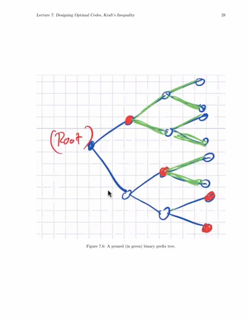
Proof. (in the forward direction) Consider a binary-tree representation of the prefix code. Because the codeis a prefix code, no codeword can be the prefix of any other. Therefore, we can prune all the branches belowa codeword node.


Figure 7.6: A pruned (in green) binary prefix tree.


Let lmax be the maximum level of the tree (the length of the longest codeword.) Each codeword at level li“knocks out” 2lmax−li descendants, so we knock out a total of

∑mi=1 2lmax−li nodes. This must be less than

the number of nodes that exist, so we get

m∑i=1

2lmax−li ≤ 2lmax . (7.4)

Dividing by 2lmax on both sides, we get Kraft’s inequality.

The converse can be shown by construction.

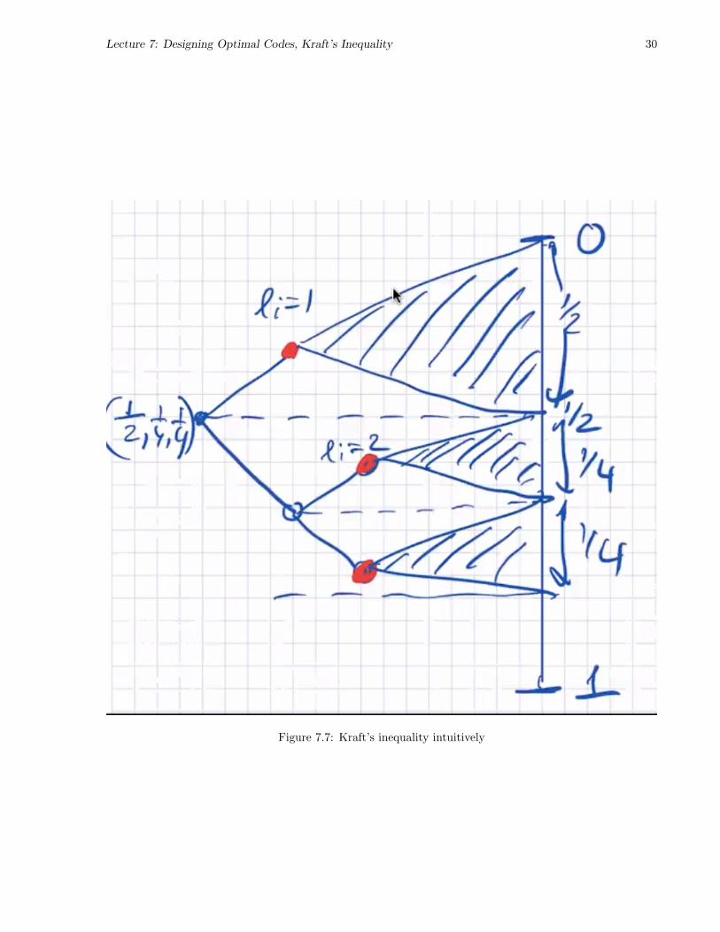
Kraft’s inequality can be intuitively understood by partitioning the probability space (the real line from 0to 1) by halves recursively: codewords at level li span a fraction 2−li of the probability space.

Now, we can rewrite our optimization problem, since Kraft’s inequality has given us a way of translating thecondition of being a prefix code into math:

min{li}

∑i

pili

s.t.li ∈ Z+,

m∑i=1

2−li ≤ 1

(7.5)

This is an integer programming problem, and it’s still not clear if it can be solved intuitively.

7.4 Coding Schemes and Relative Entropy

L =

m∑i=1

pili =

m∑i=1

pi log1

2−li(7.6)

Define

Z =∑i

2−li (7.7)

qi∆=

2−li

Z, (7.8)

where Z is defined analogous to physics-entropy as the partition function. We can rewrite the length:

L =∑i

pi log1

qiZ=∑i

pi log1

qi+∑i

pi log1

Z(7.9)

= log1

Z+∑i

pi log1

qi(7.10)


Figure 7.7: Kraft’s inequality intuitively


The log 1Z is referred to as the slack in Kraft’s inequality; if it is 0, then Kraft’s inequality is an exact equality.

We can split up the other term into absolute and relative entropies:

L =∑i

pi logpiqi

+∑i

pi log1

pi+ log

1

Z(7.11)

= D(p ‖ q) +H(X) + log1

Z. (7.12)

The slack and the relative entropy must both be nonnegative, and therefore L ≥ H(X); it’s impossible tobeat the entropy. For equality, we need Z = 1, which roughly states that the code should span the wholeprobability space (“don’t be dumb”), and we need p = q (otherwise the relative entropy will be nonzero),i.e. pi = 2−li , which gives us the condition that the probabilities must be dyadic.

Generally, to get the best code length while satisfying Kraft’s inequality, we set

li = dlog2

1

pie. (7.13)

We can show that these lengths still satisfy Kraft’s inequality:

m∑i=1

2−li =

m∑i=1

2−dlog 1

pie

(7.14)

≤m∑i=1

2log 1

pi =

m∑i=1

pi = 1. (7.15)

And we can show that this average length deviates from the entropy by at most one bit:

L = E[l(X)] ≤ E[1 + log

1

p(X)

]= 1 +H(X). (7.16)

This is not always good news if H(X)� 1; for example, if X ∼ Bern(0.0001) and H(X) ≈ 2.1× 10−5 bits.How do we reduce the one bit of redundancy? We could encode multiple symbols at once, and in generalamortize the one-bit code over n symbols to get an upper bound of 1

n .

H(X1, . . . , Xn) ≤ E[l∗(X1, . . . , Xn)] ≤ H(X1, . . . , Xn) + 1 (7.17)

H(X1, . . . , Xn)

n≤ E[l∗(X1, . . . , Xn)]

n≤ 1

n+H(X1, . . . , Xn)

n. (7.18)

For the limit as n→∞,

limn→∞

E[l∗(X1, . . . , Xn)]

n= H (7.19)

H = limn→∞

H(X1, . . . , Xn)

n. (7.20)

Therefore, we achieve the entropy rate!

Note that this is a very general result: X1, . . . , Xn are not assumed to be i.i.d. or Markov.

7.5 The price for assuming the wrong distribution

Consider expected length under p(x) of the code lengths l(x) = log 1q(x) (dropping the ceiling for simplicity).

L =∑i

pi log1

qi=∑i

pi log1

pi+∑i

pi logpiqi

(7.21)

= D(p ‖ q) +H(p). (7.22)

The cost of being wrong about the distribution is the distance (relative entropy) between the distributionyou think it is, and the distribution it actually is.

L = H + “price of being dumb” + “price of being wrong” (7.23)

32

Lecture 8: Prefix code generality, Huffman codes 33


Lecture 8: Prefix code generality, Huffman codesLecturer: Kannan Ramchandran 22 September Aditya Sengupta

In case a prefix code satisfies Kraft’s inequality exactly, i.e.∑i 2−li = 1, we call it a complete prefix code.

Since we’ve decided to restrict our attention to prefix codes, we might expect that we lose some optimalityor efficiency by making this choice. However, prefix codes are actually fully optimal and efficient, i.e. thegeneral class of uniquely decodable codes offers no extra gain over prefix codes. We formalize this:

Theorem 8.1 (McMillan). The codeword lengths of any UD binary code must satisfy Kraft’s inequality.Conversely, given a set of lengths {li} satisfying Kraft’s inequality, it is possible to construct a uniquelydecodable code where the codewords have the given code lengths.

The backward direction is done already, because we know this is true of prefix codes, and prefix codes are asubset of uniquely decodable codes.

Proof. Consider Ck to be the kth extension of the base (U.D.) code C formed by the concatenation of krepeats of the base code C. By definition, if C is U.D., so is Ck.

Let l(x) be the codelength of C. For Ck, the length of the codeword is

l(x1, x2, . . . , xk) =

k∑i=1

l(xi). (8.1)

We want to show that∑i 2−li ≤ 1. The trick is to consider the kth power of Kraft’s inequality:

(∑i

2−li

)k=∑x1

∑x2

· · ·∑xk

2−l(x1)−l(x2)−···−l(xk) (8.2)

=∑

x1,x2,...,xk∈Xk

2−l(x1,...,xk) (8.3)

Suppose lmax is the longest codelength in C. Then

(∑i

2−li

)k=

klmax∑m=1

a(m)2−m, (8.4)

where a(m) represents the number of code sequences of length m. a(m) ≤ 2m, because a code sequence oflength m has 2m possible choices and in general not all of these sequences are used. Therefore

(∑i

2−li

)k≤klmax∑m=1

1 = klmax. (8.5)

Lecture 8: Prefix code generality, Huffman codes 34

Therefore

(∑i

2−li

)k≤ klmax. (8.6)

Since this has to work for any k, and in general exponential terms are faster than linear terms, the onlyway for this inequality to be satisfiable is if the base for the exponentiation is less than or equal to 1. Moreconcretely,

∑i

2−li ≤ (klmax)1/k. (8.7)

This should be satisfiable in the limit k →∞, and we can show that limk→∞

(klmax)1/k = 1.

8.1 Huffman codes

We have seen that L = E[l∗] ≥ H(X), but can we find l∗ efficiently?

Recall that our general optimization problem requires that we minimize∑x p(x)l(x) such that l(x) ∈ Z+

and such that Kraft’s inequality is satisfied. To design the code, we make the following observations:

• We want the highest-probability codewords to correspond to the shortest codelengths; i.e. if i < j =⇒pi ≥ pj then i < j =⇒ li ≤ lj . This is provable by contradiction.

• If we use all the leaves in the prefix code tree (and we should), then the deepest two leaves will be onthe same level, and therefore the two longest codewords will differ only in the last bit.

This gives rise to Huffman’s algorithm:

1. Take the two least probable symbols. They correspond to the two longest codewords, and differ onlyin the last bit.

2. Combine these into a “super-symbol” with probability equal to the sum of the two individual proba-bilities, and repeat.

Example 8.1. Let X = {a, b, c, d, e} and PX = {0.25, 0.25, 0.2, 0.15, 0.15}.

Figure 8.8: Example Huffman encoding

The average length of this encoding is L = 2.3, and the entropy is around H(X) =2.28.

�

8.2 Limitations of Huffman codes

“you know how they say ’I come to bury Caesar, not to praise him’? I’ve come here to kill Huffman codes.”- Prof. Ramchandran

There are several reasons not to like Huffman codes.

1. Computational cost: the time complexity of making the Huffman tree is O(m logm) where |X | = m.For a block of length n, the alphabet size is mn, and so this gets painful quickly.

2. They are designed for a fixed block length, which is not a widely applicable assumption

3. The source is assumed to be i.i.d., and non-stationarity is not handled.

To address this, we’ll introduce concepts like arithmetic coding.

35

Lecture 9: Arithmetic coding 36


Lecture 9: Arithmetic codingLecturer: Kannan Ramchandran 24 September Aditya Sengupta

9.1 Overview and Setup, Infinite Precision

Arithmetic coding is a (beautiful!) entropy coding scheme for compression that operates on the entire sourcesequence rather than one symbol at a time. It takes in a message all at once, and returns a binary bitstreamcorresponding to it.

Consider a source sequence, such as “the quick brown fox jumps over the lazy dog”. Suppose this hassome encoding to a binary string, such as 011011110110000. We can interpret this as a binary fraction byprepending a 0., so that we get 0.011011110110000, a number in [0, 1). Note that these are binary fractions,so 0.01 represents 1

4 .

The key concept behind arithmetic coding is that we can separate the encoding/decoding aspects from theprobabilistic modeling aspects without losing optimality.

Example 9.1. Consider a dyadic distribution, X ∼ p, X = {1, 2, 3, 4}, pX = { 12 ,

14 ,

18 ,

18}. We write

the CDF in terms of binary fractions; in general if we want to represent the interval[a, b) we’d like to choose a binary fraction that corresponds to a, and such thatthe number of bits used corresponds to the length b − a. For example, the lengthspanned by x = 2 is 1

4 and so we want − log 14 = 2 bits.

FX(x) =

0.0 x = 1

0.10 x = 2

0.110 x = 3

0.111 x = 4

(9.1)

Further, we can continue subdividing each interval to assign longer messages! Forexample, if we subdivide [0, 1/2), we can assign codewords to messages starting with1, i.e. “11′′ → [0, 1/4), “12′′ → [1/4, 1/8) and so on.

�

In the limit, the subinterval representing (X1, X2, . . . , Xn) shrinks to a single point.

Definition 9.1. Given a sequence of RVs X1, X2, · · · ∼ p over X = {0, 1} where Xi ∼ Bern(p), thearithmetic code for x = 0.X1X2 . . . is

FX(x) = U = 0.U1U2U3 . . . , (9.2)

where U1, U2, . . . are the encoded symbols for X1, X2, . . . and FX(x) = P(X < x).

Theorem 9.1. The arithmetic code F achieves the optimal compression rate. Equivalently, the encodedsymbols U1, U2, . . . are i.i.d. Bern(1/2) RVs and cannot be further compressed.

Lemma 9.2. If X is a continuous RV with cdf F , then FX(x) ∼ Unif [0, 1].

Proof. Let U ∼ Unif [0, 1]:

P(U ≤ u) = P(FX(x) ≤ u) = P(X ≤ F−1X (u)) = FX(F−1

X (u)). (9.3)

The proof of the theorem is in C&T probably.

9.2 Finite Precision

Suppose we have X = {A,B,C} and pX = {0.4, 0.4, 0.2}. Suppose we want to encode ACAA.

We assign A→ [0, 0.4), B → [0.4, 0.8), C → [0.8, 1). The encoding of A gives us the interval [0, 0.4), and wefurther subdivide this interval. The next symbol is a C so we get the interval [0.32, 0.4) (this encodes thedistribution X2|X1, in general the second symbol’s distribution doesn’t have to be the same distribution asthe first). The next A gives us [0.32, 0.352), and the final A gives us [0.32, 0.3328). Finally, we reserve acode symbol for the end of a string, so that we know exactly when a string ends.

The subinterval’s size represents P(ACAA) = P(X1 = A)P(X2 = C|X1 = A)P(X3 = A|X1X2 = AC)P(X4 =A|X1X2X3 = ACA). Note that we can capture arbitrary conditioning in the encoding!

9.3 Invertibility

We can show that l(Xn) ≤ log 1p(Xn) + 2.

We can use a Shannon-Fano-Elias code argument to show this: for any message, the binary interval corre-sponding to it must fully engulf the probability interval of the sequence. The +2 comes from ensuring thatthe interval represented by the code is fully inside the probability interval of the sequence, for which we mayhave to subdivide twice.

If we have a source interval with a marginally smaller probability than the optimal coding interval size,there’s no way to identify whether the interval belongs to the source interval or those above/below it givenjust the coding interval. When we divide it in half, the top and bottom halves still have ambiguity: in orderto ensure there’s an interval that is unambiguously within the optimal interval, we need to divide twice anduse the two “inner” midpoints.

37

Lecture 10: Arithmetic coding wrapup, channel coding 38

Figure 10.9: Channel diagram


Lecture 10: Arithmetic coding wrapup, channel codingLecturer: Kannan Ramchandran 29 September Aditya Sengupta

Arithmetic coding has several advantages over, e.g., Huffman codes:

1. Complexity: to communicate a string of N symbols from an alphabet of size |X | = m, both theencoder and the decoder need to compute only Nm conditional probabilities Contrast this cost withthe alternative of using a large block-length Huffman code, where all the possible block sequences haveto have their probabilities evaluated.

2. Flexibility: can be used with any source alphabet and any encoded alphabet.

3. Arithmetic coding can be used with any probability distribution that can change from context tocontext.

4. Can be used in a “universal” way. Arithmetic coding does not require any specific method of generatingthe prediction probabilities, and so these may be naturally produced using a Bayesian approach. Forexample, if X = {a, b}, Laplace’s rule gives us that P(a|x1, x2, . . . , xn−1) = Fa+1

Fa+Fb+2 (where Fa, Fb are

the number of occurrences so far of a and b.) Thus the code adapts to the true underlying probabilitydistribution.

10.1 Communication over noisy channels

Consider a block diagram source-to-encoder-to-noisy-channel-to-decoder-to-reconstructed-source.

Even though the channel is noisy, we would like to ensure that there is no noise induced overall between thesource encoder and source decoder, while maximizing the channel’s capacity, i.e. the maximum number ofbits per use of the channel such that communication remains reliable.

Say we give the channel an input W and that the output is W . We can say the channel takes in and spitsout bits, which means we need to add an encoder before the channel and a decoder after.

1. The encoder converts W ∼ U [0, 2m − 1] (an optimally compressed source with m bits) to a string of nbits X1, . . . , Xn.

2. The channel takes in this sequence of bits and returns corrupted bits Y1, . . . , Yn following the probabilityP(Y1, . . . , Yn|X1, . . . , Xn).

3. The decoder takes in the corrupted bits and outputs the optimal decoding W .

We define two metrics to assess channel performance:

1. Probability of error, Pe = P(W 6= W )

2. Rate R = log2 Mn = m

n .

Communication is an optimization problem between these two factors. We can find an optiml probability oferror for a fixed data rate R and length |W |: P (err)∗ = minf,g P (err), where f and g are the encoder anddecoder.

The simplest possible strategy is a repetition code, where each encoded symbol is sent n times. Supposethe channel is a BEC(p). The probability of error is Pe = 1

2pn (every single bit needs to be erased), and

the rate is R = 1n . The rate is low while the probability of error is also low; we’d like to bring the rate up

without increasing Pe much.

Shannon showed that at some value of the rate, Pe goes to zero and reliable communication is possible.

39

Lecture 11: Channel coding efficiency 40


Lecture 11: Channel coding efficiencyLecturer: Kannan Ramchandran 1 October Aditya Sengupta

We’re going to focus on the discrete memoryless channel, with the property that P(Y n|Xn) =∏ni=1 P(yi|xi).

The capacity of a channel is C = maxp(x) I(X;Y ). This is intuitively something we want to maximize: wewant to make it so that the output tells us as much as possible about the input. The channel is specified bythe joint distribution p(x, y), in which p(x) is to be designed (based on how the encoder works) and p(y|x)is fixed (it characterizes the channel).

Example 11.1. Consider a noiseless channel, where H(Y |X) = 0. If X ∼ Bern(1/2) then themaximum is achieved: C = maxp(x)H(X) = 1.

�

11.1 Noisy typewriter channel

Suppose X = {A,B,C,D}, and the channel takes each letter to itself with probability 1/2 and to its nextneighbor (D going to A) with probability 1/2.

Due to this symmetry, H(Y |X) = 1, and so to maximize the capacity we want to maximize H(X). In theuniform case, this comes to C = 2− 1 = 1.

For a BSC with flip probability p, the channel capacity is 1−H(p), because the maximum initial entropy is1 and the minimum conditioned flip entropy is H(p).

For a BEC, H(X) = H2(α) (where α is a starting Bernoulli parameter), and for the conditional entropy:

H(X|Y = 0) = 0 (11.1)

H(X|Y = 1) = 0 (11.2)

H(X|Y = e) =∑

x∈{0,1}

p(x|Y = e)1

log p(x|Y = e)(11.3)

= (1− α) log1

1− α+ α log

1

α(11.4)

Therefore the capacity is

C = maxp(x)

H2(α)− pH2(α) = 1− p. (11.5)

Theorem 11.1 (Shannon: Channel Coding). Any rate R < C is achievable, meaning that there exists ascheme for communication at rate R such that Pe → 0. Conversely, if R > C, Pe is strictly bounded awayfrom 0.

41

Lecture 12: Rate Achievability 42


Lecture 12: Rate AchievabilityLecturer: Kannan Ramchandran 6 October Aditya Sengupta

Shannon’s capacity achievability argument will end up concluding that the capacity of a BEC(p) cannotexceed 1−p, but that the capacity 1−p is achievable. Even with the aid of a “feedback oracle”, the capacityof a BEC(p) is at most 1− p.

To prove the achievability, make a codebook. Let R = logMn and M = 2nR. Write a codebook with n−length

codewords for each of the M possible messages, and use the encoding scheme that we saw in 126 (just copythat over). The probability of error with this encoding scheme is

Pe = Ec[Pe(c)] =∑c∈C

P(C = c)P(W 6= W |c) (12.1)

=∑c

P(W 6= W,C = c) (12.2)

= P(W 6= W ). (12.3)

The channel action is as follows:

1. The encoder and decoder generate a random codebook C based on iid fair coin flips ∼ Bern(1/2).

2. A message W is chosen at random from [M ].

3. The wth codeword ~cw = (ciw) is transmitted over the BEC(p) channel.

4. The receiver gets Y n according to P(Y n|Xn).

5. Decoding rule: if there is exactly one codeword consistent with the received Y n, then declare themessage associated with that codeword as the decoded message; else, declare error.

Example 12.1. Suppose M = 4, R = 12 , and the codebook is

1 2 3 41 0 0 0 02 0 1 1 03 1 0 0 14 1 1 1 1

Here, if we send 0000, that gets uniquely decoded as 1.

If we send 0ee0, it is uncertain whether the message was 1 or 2, so an error isdeclared.

�

The probability of error is then

Pe = P(W 6= W ) = P(W 6= 1|W = 1) (12.4)

= P(∪Mw=2xn(w) = xn(1) in all the unerased bit locations) ≤

M∑w=2

P(xn(w) = xn(1) in all the unerased bit locations) < MP(W = 2|W = 1).

(12.5)

By LLN, the number of erasures tend to np with probability 1, and so the number of unerased bit locationstends to n(1− p) with probability 1. Since each bit is independently generated with probability 1

2 , we have

P(W = 2|W = 1) =1

2n(1−p) (12.6)

And therefore

Pe < 2nR2−n(1−p) = 2−n((1−p)−R) (12.7)

Therefore, as n→∞, Pe → 0 if 1− p > R. Therefore, for any ε > 0, R = 1− p− ε is achievable.

43

Lecture 13: Joint Typicality 44


Lecture 13: Joint TypicalityLecturer: Kannan Ramchandran 8 October Aditya Sengupta

We know what typicality with respect to one sequence means; now we look at typicality with a set of multiplesequences. We’ve already seen what a typical sequence of RVs is, and in particular we saw the definition ofa width-ε typical set:

A(n)ε = {xn | | log p(xn) + nH(X)| ≤ nε}. (13.1)

For what follows, denote typicality by saying p(xn) ∼ 2−nH(X).

Now, we extend this:

Definition 13.1. For iid RVs Xn and iid RVs Y n, (xn, yn) is called a jointly typical sequence if

p(xn) ∼ 2−nH(X) (13.2)

p(xn) ∼ 2−nH(Y ) (13.3)

p(xn, yn) ∼ 2−nH(X,Y ). (13.4)

13.1 BSC Joint Typicality Analysis

Consider a BSC(p) where X ∼ Bern(1/2), i.e. the output Y is related to the input X by

Y = X ⊕ Z (13.5)

where Z ∼ Bern(p).

The joint entropy is

H(X,Y ) = H(X) +H(Y |X) = 1 +H2(p) (13.6)

Let (xn, yn) be jointly typical. Then, p(xn) ∼ 2−n, p(yn) ∼ 2−n, and p(xn, yn) ∼ 2−n(1+H2(p)).

From the asymptotic equipartition property (almost all the probability space is taken up by typical se-quences), we get that

|{xn | p(xn) ∼ 2−n} ∼ 2n (13.7)

|{yn | p(yn) ∼ 2−n} ∼ 2n (13.8)

|{(xn, yn) | p(xn, yn) = 2−n(1+H2(p))}| ∼ 2n(1+H2(p)) � 22n. (13.9)

Lecture 13: Joint Typicality 45

Next, consider the conditional distribution: for jointly typical (xn, yn),

p(yn|xn) =p(xn, yn)

p(xn)∼ 2−nH(X,Y )

2−nH(X)(13.10)

and so, for jointly typical (xn, yn),

p(yn|xn) ∼ 2−nH(Y |X) (13.11)

If you imagine a space of all the possible sequences xn, you can draw “noise spheres” of typical sequencesthat are arrived at by going through the BSC. The size of these noise spheres is

(nnp

)≈ 2nH2(p) by Stirling’s

approximation.

The number of disjoint noise spheres (each corresponding to a single transmitted codeword xn(ω)) is lessthan or equal to 2nH(Y )/2nH(Y |X) = 2nI(X;Y ). Therefore, the total number of codewords M is

M = 2nR ≤ 2nI(X;Y ) (13.12)

and so

log2M

n= R ≤ I(X;Y ) = C. (13.13)

We have therefore shown that rates of transmission over the BSC necessarily satisfy R ≤ C. Now, we showthat any R ≤ C is achievable. This can be done by the same codebook argument as for the BSC. Thereceiver gets Y n = Xn(ω)⊕ Zn. Without loss of generality, we’ll assume W = 1 was sent.

From there, the decoder does typical-sequence decoding: it checks whether (Xn(1), Y n) is jointly typical.Let Zni be the noise candidate associated with message i.

We can see that

Zni = Xi(1)⊕ Y i ∀i ∈ {1, . . . ,M} (13.14)

This gives us a sequence of noise values, and we want this sequence to look like Bern(1/2).

Therefore, our decoding rule is as follows: the decoder computes yn ⊕ xn(w) for all w ∈ {1, 2, . . . ,M}.Eliminate all w that Y n ⊕Xn(w) 6∈ A(n)

ε . If only one message survives, declare it the winner. Else, declareerror.

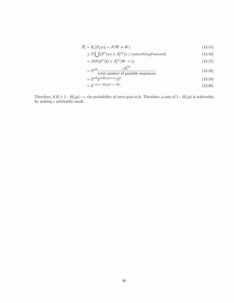
Pe = Ec[Pe(c)] = P (W 6= W ) (13.15)

≤ P(⋃{Zn(w) ∈ A(n)

ε }) ∪ (somethingImissed) (13.16)

< MP(Zn(2) ∈ A(n)ε |W = 1) (13.17)

= 2nR|A(n)ε

total number of possible sequences(13.18)

= 2nR2n(H2(p)+1)/2n (13.19)

= 2−n(1−H2(p)−ε−R). (13.20)

Therefore, if R < 1−H2(p)−ε, the probability of error goes to 0. Therefore, a rate of 1−H2(p) is achievableby making ε arbitrarily small.

46


Lecture 14: Fano’s Inequality for ChannelsLecturer: Kannan Ramchandran 12 October Aditya Sengupta

I missed this lecture and later referred to the official scribe notes.

47

Lecture 15: Polar Codes, Fano’s Inequality 48


Lecture 15: Polar Codes, Fano’s InequalityLecturer: Kannan Ramchandran 15 October Aditya Sengupta

15.1 Recap of Rate Achievability

Fano’s inequality tells us that for any estimator X such that X → Y → X is a Markov chain with Perr =P(X 6= X),

H2(Pe) + Pe log |X | ≥ H(X|Y ). (15.1)

To prove the converse for random coding, that R ≤ C is achievable, we set up the Markov chain W → Xn →Y n → W :

nR = H(W ) = I(W ; W ) +H(W |W ) (15.2)

≤ I(Xn;Y n) + 1 + P (n)e nR (15.3)

Therefore R ≤ C + 1n +RP

(n)e ; in the limit n→∞, P (n)

e → 0.

15.2 Source Channel Theorem

Theorem 15.1. If V1, . . . Vn is a finite-alphabet stochastic process for which H(ν) < C, there exists asource-channel code with Perr → 0.

Conversely, for any stationary process, if H(ν) > C then Perr is bounded away from zero, and it is impossibleto transmit the process over the channel reliably (i.e. with arbitrarily low Perr).

Proof. For achievability, we can use the two-stage separation scheme: Shannon compression and communi-cation using random codes. If H(ν) < C, reliable transmission is possible.

For the converse, we want to show that P(V n 6= V n) → 0 implies that H(ν) ≤ C for any sequence ofsource-channel codes:

Xn(νn) : V n → Xn (15.4)

gn(Y n) : Yn → V n (15.5)

Consider the Markov chain V n → Xn → Y n → V n. Fano’s inequality tells us

Lecture 15: Polar Codes, Fano’s Inequality 49

H(V n|V n) ≤ 1 + P (V n 6= V n) log |νn| = 1 + P (V n 6= V n)n log |ν|. (15.6)

For a source channel code:

H(ν) ≤ H(V1, . . . , Vn)

n=H(V n)

n(15.7)

=1

n

[H(V n|V n) + I(V n; V n)

](15.8)

≤ 1

n

[1 + P(V n 6= V n)n log |ν|+ I(Xn;Y n)

](15.9)

≤ 1

n+ P(V n 6= V n) log |ν|+ C (15.10)

If we let n→∞, then P(V n ≤ V n) = 0 and therefore H(ν) ≤ C.

15.3 Polar Codes

Polar codes were invented by Erdal Arikan in 2008. They achieve capacity with encoding and decodingcomplexities of O(n log n), where n is the block length.

Among all channels, there are two types of channels for which it’s easy to communicate optimally:

1. The noiseless channel, X − Y ; Y determines X.

2. The useless channel, X Y ; Y |= X.

In a perfect world, all channels would be one of these extremal types. Arikan’s polarization is a technique toconvert binary-input channels to a mixture of binary-input extremal channels. This technique is information-lossless and is of low complexity!

Consider two copies of a binary input channel, W : {0, 1} → Y . The first one takes in X1 and returns Y1

and the second takes in X2 and returns Y2.

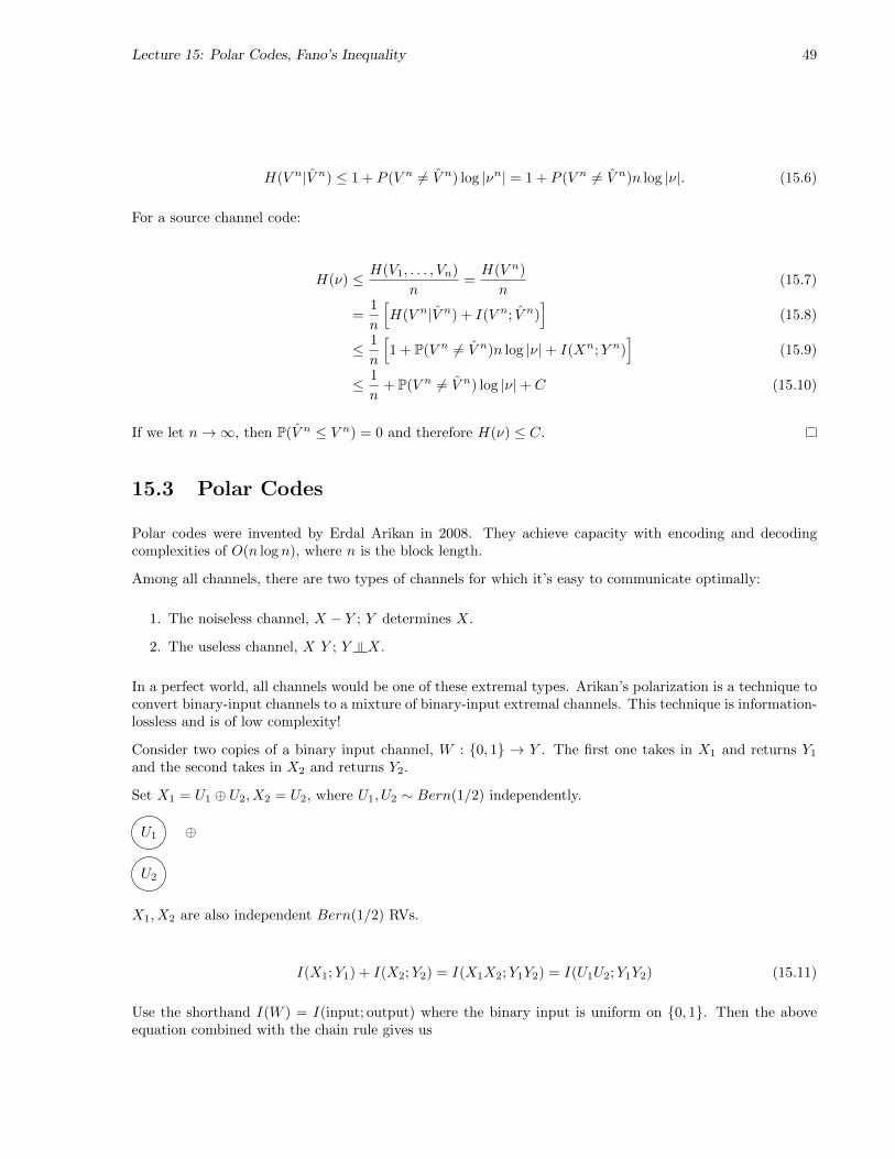
Set X1 = U1 ⊕ U2, X2 = U2, where U1, U2 ∼ Bern(1/2) independently.

U1

U2

⊕

X1, X2 are also independent Bern(1/2) RVs.

I(X1;Y1) + I(X2;Y2) = I(X1X2;Y1Y2) = I(U1U2;Y1Y2) (15.11)

Use the shorthand I(W ) = I(input; output) where the binary input is uniform on {0, 1}. Then the aboveequation combined with the chain rule gives us

2I(W ) = I(U1;Y1Y2) + I(U2;Y1, Y2|U1) (15.12)

We can rewrite the second term as

2I(W ) = I(U1;Y, Y2) + I(U2;Y1, Y2, U1) (15.13)

Denote the first term by I(W−) and the second by I(W+):

2I(W ) = I(W−) + I(W+). (15.14)

We’ll now show two things:

1. W− and W+ are associated with particular channels that satisfy the extremal property we saw before.

2. I(W−) ≤ I(W ) ≤ I(W+).

Given the mutual information expressions, the channel W− takes in as input U1 and outputs (Y1, Y2). U2 isalso an input but we’re not looking at it for now, I think.

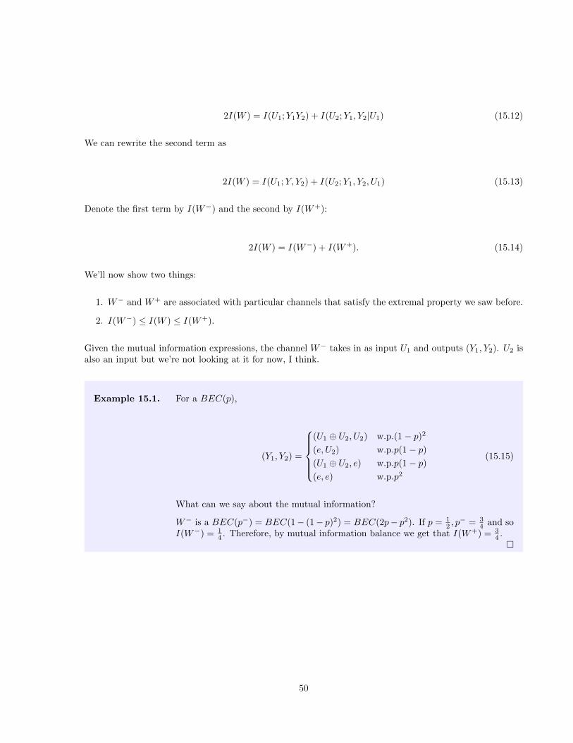
Example 15.1. For a BEC(p),

(Y1, Y2) =

(U1 ⊕ U2, U2) w.p.(1− p)2

(e, U2) w.p.p(1− p)(U1 ⊕ U2, e) w.p.p(1− p)(e, e) w.p.p2

(15.15)

What can we say about the mutual information?

W− is a BEC(p−) = BEC(1− (1− p)2) = BEC(2p− p2). If p = 12 , p− = 3

4 and soI(W−) = 1

4 . Therefore, by mutual information balance we get that I(W+) = 34 .�

50

Lecture 16: Polar Codes 51


Lecture 16: Polar CodesLecturer: Kannan Ramchandran 27 October Aditya Sengupta

Recall that the polar transform changes assumed Bern(1/2) random variables U1, U2 to X1, X2 by therelationship X1 = U1 ⊕ U2, X2 = U2.

We showed last time that

2I(X1;Y1) = I(U1, U2;Y1, Y2) = I(U1;Y1, Y2) + I(U2;Y1, Y2|U2), (16.1)

and we can write this as the combination of two channels:

2I(W ) = I(W−) + I(W+). (16.2)

W− is a worse channel than W , and W+ is a better channel than W .

Suppose W is a BEC(p); we can then show that W− is a BEC(2p− p2). Similarly, we can look at W+:

I(W+) : U2 → Y1Y2U2 (16.3)

(Y1, Y2, U1) =

(U1 ⊕ U2, U2, U1) w.p.(1− p)2

(e, U2, U1) w.p.p(1− p)(U1 ⊕ U2, e, U1) w.p.(1− p)p(e, e, U1) w.p.p2

(16.4)

Therefore W+ is a BEC(p2), as U2 can be recovered with probability 1− p2.

We can now verify that the polar transformation preserves mutual information:

I(W−) + I(W+)

2=

1− (2p− p2) + 1− p2

2= 1− p = I(W ) (16.5)

The synthetic channels are not real, and this is fine for W−, but not for W+, since we only have U1 and notthe real U1: U1 is not actually observed by the receiver. To get around this, we impose a decoding order.

Consider a genie-aided receiver that processes the channel outputs:

U1 = φ1(Y1, Y2) (16.6)

U2 = φ2(Y1, Y2, U1) (16.7)

where U1 is perfectly known by the genie.Consider also the implementable receiver

U1 = φ1(Y1, Y2) (16.8)

U2 = φ2(Y1, Y2, U1) (16.9)

We claim that if the genie-aided receiver makes no errors, then neither does the implementable receiver.That is, the block error events {(U1, U2) 6= (U1, U2)} and {(U1, U2) 6= (U1, U2)} are identical.

If the genie is wrong, then U1 6= U1. Therefore we have an overall error: (U1, U2) 6= (U1, U2), and theimplementable receiver would have an error too. It is possible for an error in U1 to propagate, but we don’tcare about that, because in that case the genie also failed to decode U1 and so we declare an error in bothanyway.

The main idea behind polar codes is to transform message bits such that a fraction C(W ) of those bits “see”noiseless channels, whereas a fraction 1 − C(W ) of bits “see” useless channels. We can do this recursively:take two W− copies and two W+ and repeat the whole process.

Some diagrams and stuff tell us that the 4× 4 polar transform has a matrix

x1

x2

x3

x4

=

1 1 1 10 1 0 10 0 1 10 0 0 1

v1

v2

v3

v4

, (16.10)

which is the tensor operation ⊗: P4 = P2 ⊗ P2.

P4 =

[P2 P2

0 P2

]. (16.11)

In general, P2k+1 = P2k ⊗ P2k .

For concreteness, with a BEC(1/2) with three splits, we can translate it into eight channels: W+++ has aprobability of success of 0.9961.

52

Lecture 17: Information Measures for Continuous RVs 53


Lecture 17: Information Measures for Continuous RVsLecturer: Kannan Ramchandran 3 November Aditya Sengupta

We saw last time that the capacity of the Gaussian channel, Yi = Xi + Zi where Zi ∼ N (0, σ2) is

C =1

2log2(1 + SNR), (17.1)

where SNR = Pσ2 . Similarly to the discrete case, we can show any rate up to the capacity is achievable, via

a similar argument (codebook and joint typicality decoding).

Similarly as the discrete-alphabet setting, we expect 12 log(1 + SNR) to be the solution of a mutual infor-

mation maximization problem with a power constraint:

maxp(x)

I(X;Y ) s.t.E[X2] ≤ P, (17.2)

where I(X;Y ) is some notion of mutual information between continuous RVs X,Y . This motivates thefact that we need to introduce the notion of information measures, like we saw in the discrete case (mutualinformation, KL divergence/relative entropy, and entropy) for continuous random variables before we canoptimize something like Equation 17.2.

Chapter 8 of C&T has more detailed exposition on this topic.

As our first order of business, let’s look at mutual information. We can try and make a definition thatparallels the case of DRVs (discrete RVs). Recall that for DRVs X,Y ,

I(X;Y ) = E[log

p(x, y)

p(x)p(y)

](17.3)

The continuous case is similar: all we have to do is replace the PMFs p(x), p(y), p(x, y) with their PDFsf(x), f(y), f(x, y).

Definition 17.1. The mutual information for CRVs X,Y ∼ f is

I(X;Y ) , E[log

f(x, y)

f(x)f(y)

](17.4)

To show this is a sensible definition, we show it is an approximation to the discretized form of X,Y . Divideup the real line into width-∆ subintervals. For ∆ > 0, define X∆ = i∆ if i∆ ≤ X ≤ (i + 1)∆. Then, forsmall ∆,


p(X∆) ≈ ∆f(x) (17.5)

p(Y ∆) ≈ ∆f(y) (17.6)

p(X∆, Y ∆) ≈ ∆2f(x)f(y) (17.7)

Then,

I(X∆;Y ∆) = E[log

p(X∆, Y ∆)

p(X∆)p(Y ∆)

](17.8)

= E[log

f(x, y)∆2

f(x)∆f(y)∆

](17.9)

= I(X;Y ) (17.10)

Therefore, we see that

lim∆→0

I(X∆;Y ∆) = I(X;Y ) (17.11)

17.1 Differential Entropy

Once again proceeding analogous to the discrete case, we see that

I(X;Y ) = E[log

f(X,Y )

f(X)f(Y )

]= E

[log

f(Y |X)

f(Y )

](17.12)

= E[log

1

f(Y )

]− E

[1

f(Y |X)

](17.13)

We would like to define the entropy of Y to be E[log 1

f(Y )

], and the conditional entropy of Y given X to

be E[log 1

f(Y |X)

]. But we have to deal with the fact that f(Y ), f(Y |X) are not probabilities. The intuition

that entropy is the number of bits required to specify an RV breaks down, because we require infinite bits tospecify a continuous RV. But it is still convenient to have a measure for CRVs. This motivates the definitionswe’d like to have

h(Y ) , E[log

1

f(Y )

](17.14)

h(Y |X) , E[log

1

f(Y |X)

](17.15)

Remark 17.1. There are similarities and dissimilarities between H(X) and h(X).

1. H(X) ≥ 0 for any DRV X, but h(X) need not be a nonnegative quantity for any CRV, as probabilitydensity could be any positive number.


2. H(X) is label-invariant, but h(X) depends on the label. For example, let Y = aX for a scalar a.For discrete RVs, H(Y ) = H(X). However, for continuous RVs, we know that fY (y) = 1

|a|fX(ya

).

Therefore

h(Y ) = E[log

1

fY (y)

]= E

[log

|a|fX(Ya

)] (17.16)

= log |a|+ E

[log

1

fX(Ya

)] (17.17)

= log |a|+ h(X) (17.18)

Therefore h(aX) = h(X) + log a.

In the vector case, if Y = Ax, h(Ax) = log |∣∣A∣∣ |+ h(x).

17.2 Differential entropy of popular distributions

17.2.1 Uniform

Let X ∼ Unif([0, a]).

h(X) = E[log

1

f(X)

]= E

[log

1

a

]= log a. (17.19)

Note that for a < 1, log a < 0 and h(X) < 0.

For a = 1, h(X) = 0. We reconcile this in terms of physical intuition by thinking of 2h(X) = 2log a = a as themeaningful quantity: this is the volume of the support set of the RV.

We can relate differential entropy to its discrete version as well; define X∆ as above, then

H(X∆) = −∑i

pi log pi (17.20)

= −∑i

f(xi)∆ log(f(xi)∆) (17.21)

= −∑i

∆f(xi) log f(xi)−∑i

∆ log ∆ (17.22)

and as ∆→ 0, this goes to the Riemann sum, i.e.

H(X∆)→ −∫f(x) log f(x) dx−∆ log ∆ (17.23)

and so


Theorem 17.2.

lim∆→0

H(X∆) + ∆ log ∆ = h(f) = h(X). (17.24)

The entropy of an n−bit quantization of a CRV X ≈ h(X) + n. If X ∼ Unif [0, 1], h = 0, H∆ = n.

17.2.2 Normal

Let X ∼ N (0, 1).

log2

1

fX(x)=

1

2log2(2π) +

x2

2log2 e (17.25)

Therefore

h(X) =1

2log(2π) +

1

2log2 eE[X2] (17.26)

=1

2log2(2πe). (17.27)

Transformation rules tell us that if Z ∼ N (µ, σ2), then

h(Z) =1

2log 2πeσ2 (17.28)

Theorem 17.3. For a constant a, I(aX;Y ) = I(X;Y ).

Proof.

I(aX;Y ) = h(aX)− h(aX|Y ). (17.29)

We know h(aX) = h(X) + log |a|. Similarly,

h(aX|Y ) =

∫y

h(aX|Y = y)fY (y) dy (17.30)

=

∫y

(h(X|Y = y) + log |a|) fY (y) dy (17.31)

= h(X|Y ) + log |a|, (17.32)

and so

I(aX;Y ) = h(X) + log |a| − h(X|Y )− log |a| = I(X;Y ) (17.33)

17.3 Properties of differential entropy

1. The chain rule works the same way as for DRVs (exercise!)

2. For relative entropy, we naturally want to choose

D(f ‖ g) , EX∼f[log

1

g(x)

](17.34)

One of the most important properties of discrete relative entropy is its non-negativity. We’d like toknow if it holds in the continuous world. According to C&T p252, it does!

57

Lecture 18: Distributed Source Coding, Continuous RVs 58


Lecture 18: Distributed Source Coding, Continuous RVsLecturer: Kannan Ramchandran 10 November Aditya Sengupta

18.1 Distributed Source Coding

To motivate the idea of distributed source coding, consider the problem of compressing encrypted data.We start with some message X, which we compress down to H(X) bits. Then, we encrypt it using acryptographic key K. The bits are still H(X) after this.

What if we did this in reverse? Suppose we first encrypt X using the key K, and then compress the resultingmessage Y . We claim this can still be compressed down to H(X) bits. How does this work?

Slepian and Wolf considered this problem in 1973, as the problem of source coding with side information(SCSI). X,K are correlated sources, and K is available only to the decoder. They showed that if thestatistical correlation between X and K are known, there is no loss of performance over the case in which Kis known at the encoder. More concretely, if maximal rates RK , RX are achievable for compressing K andX separately, then the joint rate (RK , RX) is achievable simultaneously.

Example 18.1. Let X,K be length-3 binary data where all strings are equally likely, with thecondition that the Hamming distance between X and K is at most 1 (i.e. X andK differ by at most one bit).

Given that K is known at both ends, we can compress X down to two bits. We cando this by considering X ⊕ K and noting that this can only be 000, 100, 010, 001.Indexing these four possibilities gives us X compressed in two bits.

From the Slepian-Wolf theorem, we know that we can compress X to two bits evenif we don’t know K at the encoder. We can show this is achievable as follows:suppose X ∈ {000, 111}.

• If X = 000, then K ∈ {000, 001, 010, 100}.

• If X = 111, then K ∈ {111, 110, 101, 011}.

These two sets are mutually exclusive and exhaustive. Therefore, the encoder doesnot have to send any information that would help the decoder distinguish between000 and 111, as the key will help it do this anyway. We can use the same codewordfor X = 000 and X = 111.

Partition F32 into four cosets like this:


{000, 111} → 00 (18.1)

{001, 110} → 01 (18.2)

{010, 101} → 10 (18.3)

{100, 011} → 11 (18.4)

The index of the coset is called the syndrome of the source symbol. The encodersends the index of the coset containing X, and the decoder finds a codeword in thegiven coset that is closest to K.

�

More generally, we partition the space of possible source symbols into smaller circles. The encoder sendsinformation specifying which circle we look in, and the decoder looks within that circle and uses the key todecode the correct source symbol. The main idea here is that the key can be used to make a joint decoderand decrypter.

18.2 Differential Entropy Properties

One of the most important properties of relative entropy in the discrete case is its non-negativity. This stillholds in the continuous case:

Theorem 18.1. (C&T p252): D(f ‖ g) ≥ 0.

Proof. Similar to the discrete setting, let f, g be the two PDFs and let S be the support set of f .

D(f ‖ g) = EX∼f[log

f(x)

g(x)

](18.5)

= EX∼f[− log

g(x)

f(x)

](18.6)

≥ − logEX∼f[g(x)

f(x)

](Jensen’s) (18.7)

= − log

[∫x∈S

f(x)g(x)

f(x)dx

](18.8)

= − log

[∫x∈S

g(x) dx

](18.9)

≥ 0 (18.10)

The argument of the integral is less than or equal to 1, so its negative log must be nonnegative.

Corollary 18.2. For CRVs X and Y ,

I(X;Y ) ≥ 0. (18.11)


Proof.

I(X;Y ) = D(fXY (x, y) ‖ fX(x)fY (y)) ≥ 0 (18.12)

Corollary 18.3. For CRVs X and Y ,

h(X|Y ) ≤ h(X), (18.13)

and h(X|Y ) = h(X) iff X |= Y .

Theorem 18.4. h(X) is a concave function in X.

Proof. Exercise.

18.3 Entropy Maximization

We have seen that if an RV X has support on [K] = {1, . . . ,K}, and X ∼ p, then the discrete distributionp maximizing H(X) is the uniform distribution, i.e. P(X = i) = 1

K for all 1 ≤ i ≤ K. We can prove this asa theorem:

Theorem 18.5. For a given alphabet, the uniform distribution achieves maximum entropy.

We have seen this proof before, but we repeat it so that we have a proof technique we can extend to thecontinuous setting.

Proof. Let U be the uniform distribution on [K]. Let p be an arbitrary distribution on X.

D(p ‖ U) ≥ 0, X ∼ p (18.14)

D(p ‖ U) =∑x

p(x) logp(x)

U(x)(18.15)

=∑x

p(x) log p(x) +∑x

p(x) log1

U(x)(18.16)

= −H(X)−∑x

log[U(x)] · p(x) (18.17)

= −H(X)− log[U(x)]∑x

p(x)︸︷︷︸1

(18.18)

= −H(X)−∑x

U(x) logU(x)︸︷︷︸−H(U)

(18.19)

= −H(X) +H(U). (18.20)


Therefore

D(p ‖ U) = H(U)−H(X) ≥ 0, (18.21)

and so

H(U) ≥ H(X) (18.22)

Now, we can do the analogous maximization in the continuous case. However, we need to add a constraint:over all distributions on the reals, maxf h(X)→∞ (for example, if we take X ∼ U [0, a], then h(X) = log awhich blows up as a→∞.)

Therefore, the analogous problem is

maxf

h(X) s.t.E[X2] ≤ α. (18.23)

Theorem 18.6. The Gaussian pdf achieves maximal differential entropy in 18.23 subject to the secondmoment constraint.

Proof. This follows similarly to the discrete case and the uniform distribution. Note that this is essentially“guess-and-check”: to optimize without knowing up front that the Gaussian is the answer, we could useLagrange multipliers, but these become unwieldy and difficult.

Let φ(x) = 1√2πe−x

2/2, the pdf of the standard normal, and let f be an arbitrary pdf on X.

D(f ‖ φ) = EX∼f[log

f(x)

φ(x)

](18.24)

= EX∼f [log f(x)] + EX∼f log1

φ(X)(18.25)

(18.26)

The first term is just −h(X). Looking at only the second term (and integrating implicitly over all the reals)

EX∼f[log

1

φ(x)

]=

∫f(x) log

1

φ(x)dx (18.27)

=

∫f(x)

[log√

2π + (log2 e)x2

2

]dx (18.28)

=1

2log(2π)

∫f(x) dx+

∫f(x)(log2 e)

x2

2dx (18.29)

=1

2log(2π) +

log2 e

2E[X2]︸︷︷︸α

(18.30)


Since we make the constraint an equality (force EX ∼ f [X2] = α to avoid any slack), we can say that

EX∼f [X2] = EX∼φ[X2], (18.31)

and since E[log 1φ(x) ] depends only on E[X2], in the original relative entropy statement we can replace X ∼ f

with X ∼ φ, and so

D(f ‖ g) = −h(X) + h(XG) ≥ 0. (18.32)

Therefore h(XG) ≥ h(X) as desired.

18.4 Gaussian Channel Capacity Formulation

Recall that the Gaussian channel problem was to maximize capacity subject to a power constraint:

C = maxp(x)

I(X;Y ) (18.33)

s.t.E[X2] ≤ P, (18.34)

where Y = X + Z where Z ∼ i.i.d.N (0, σ2).

Notice that the power constraint is exactly the second moment constraint we just saw. It is equivalent torequire that E[X2] = P . Consider the objective:

I(X;Y ) = h(Y )− h(Y |X) (18.35)

= h(Y )− h(X + Z|X) (18.36)

= h(Y )− h(Z|X) (18.37)

= h(Y )− h(Z), (18.38)

where the last step follows because Z |= X. h(Z) is fixed, so an equivalent problem is

maxf

h(Y )s.t.E[X2] = P (18.39)

or, writing Y = X + Z and using the independence of X and Z again,

maxf

h(X + Z)s.t.E[(X + Z)2] = P + σ2 (18.40)

From the derivation of the entropy-maximizing continuous distribution, the entropy of X + Z subject to asecond-moment constraint being maximal implies that X + Z is Gaussian. We know that Z is Gaussian aswell, so X has to be Gaussian. Using linearity of independent variance, we find that X ∼ N (0, P ). Therefore

I(X;Y ) = h(XG + Z)− h(Z) (18.41)

=1

2log[2πe(P + σ2)]− 1

2log[2πeσ2] (18.42)

=1

2log

(1 +

P

σ2

), (18.43)

which was Shannon’s original formula.

63

Lecture 19: Maximum Entropy Principle, Supervised Learning 64


Lecture 19: Maximum Entropy Principle, Supervised LearningLecturer: Kannan Ramchandran 12 November Aditya Sengupta

Let X be a continuous RV with differential entropy h(X). Let X be an estimate of X and let E[(X − X)2]be the expected MSE.

Theorem 19.1. The MSE is lower-bounded by

E[(X − X)2] ≥ 1

2πe22h(X) (19.1)

with equality iff X is Gaussian and X is the mean of X.

Proof. Let X be any estimator of X.

E[(X − X)2] ≥ minX

E[(X − X)2] (19.2)

= E[(X − E[X])2] (19.3)

= var(X) (19.4)

≥ 1

2πe22h(X) (19.5)

If var(X) = σ2, then for any RV X with that variance we know that h(X) ≤ h(XG) = 12 log

(2πeσ2

).

Therefore

σ2 ≥ 22h(X)

2πe(19.6)

19.1 The principle of maximum entropy

Given some constraints on an underlying distribution, we should base our decision on the distribution thathas the largest entropy. We can use this principle for both supervised and unsupervised tasks. However, wehave access to only a few samples, which are not enough to learn a high-dimensional probability distributionfor X.

The idea for how to resolve this is we want to limit our search to a candidate set: we want to findmaxpX∈ΓH(X). We look at the exponential family:

Γ = {pX | E[γi(X)] = αi; i = 1, 2, . . . ,m} (19.7)

Lecture 19: Maximum Entropy Principle, Supervised Learning 65

Let p∗ be the max-ent distribution over Λ and let q be any distribution. Using the same decomposition aslast time,

0 ≤ D(q ‖ p∗) = −H(X) + EX∼q[log

1

p(X)

]. (19.8)

If we can show that EX∼q[log 1

p(X)

]= EX∼p∗

[log 1

p(X)

]then we can conclude that H(X) ≤ H(X∗)

To do this, we can pick a p∗(x) such that log 1p∗(x) has the exact same functional form as the constraint set

Γ.

(some stuff skipped)

Theorem 19.2. If for coefficients λ0, . . . , λm, p∗ defined as follows satisfies the constraints given for Λ,then p∗ ∈ Λ is the max-ent distribution.

p∗(x) = exp{λ0} (19.9)

some stuff here

19.2 Supervised Learning

Suppose we have a feature vector ~X = (X1, . . . , Xp) and want to predict a target variable Y . If Y ∈ R wehave a regression problem; if Y is discrete we have a classification problem.

A sensible extension of the max-ent principle to the supervised setting is

maxp ~X,Y ∈Γ

H(Y | ~X) (19.10)

For concreteness, let’s look at logistic regression. This part of the lecture was essentially a later homeworkproblem, so I’ll just present that. The problem required that we show that maximizing the conditionalentropy is equivalent to solving a logistic regression problem (with constraints on the first and second ordermoments).

We apply the maximum entropy principle. We have constraints on E[XiXj ] and on E[XiY ]; we only want toconsider the latter, as this is a conditional density and so the former terms can be put into the normalizingconstant. The optimal distribution has the form

p∗(y|x) = exp

(λ0(x) +

∑i

λ1(xi)

)(19.11)

Further, since we only have first-order dependence in the constraints that involve y,∑i λ1(xi) = eλ

ᵀx (wehave linear dependence). Therefore

p∗(y|x) = g(x)eyλᵀx (19.12)

To compute the normalizing constant, take y = 0 and y = 1 and require that they sum to 1:

g(x)(

1 + eλᵀx)

= 1 (19.13)

Therefore, the optimal distribution is

p∗(y|x) =eyλ

ᵀx

1 + eλᵀx(19.14)

66

Lecture 20: Fisher Information and the Cramer-Rao Bound 67


Lecture 20: Fisher Information and the Cramer-Rao BoundLecturer: Kannan Ramchandran 17 November Aditya Sengupta

A standard problem in statistical estimation is to determine the parameter of a distribution from a sampleof data, e.g. X1, . . . , Xn ∼ N(θ, 1). The MMSE of θ is

Xn =1

n

∑i

Xi. (20.1)

Here, we’ll give information-theoretic foundations to this.

Definition 20.1. Let {f(x; θ)} denote an indexed family of densities, such that f(x; θ) ≥ 0 and∫f(x; θ)dx =

1 for all θ ∈ Θ, where Θ is the parameter set.

Definition 20.2. An estimate for θ given a sample size n is a function T : Xn → Θ.

We want to ensure the estimator approximates the value of the parameter, i.e. T (Xn) ≈ θ.

Definition 20.3. The bias of an estimator T (X1, . . . , Xn) for the parameter θ is defined as Eθ[T (X1, . . . , Xn)−θ] (taking the expectation with respect to the density corresponding to the indexed θ.)

The estimate is unbiased if Eθ[T (·)− θ]. An unbiased estimator is good, but not good enough. We also wanta low estimation error, and this error should go to 0 as n→∞.

Definition 20.4. An estimator T (X1, . . . , Xn) for θ is said to be consistent in probability if T (X1, . . . , Xn)→θ in probability as n→∞.

We are also interested in the finite-n case:

Definition 20.5. An estimator T1(X1, . . . , Xn) is said to dominate another estimator T2(X1, . . . , Xn) if forall θ ∈ Θ,

E[(T1(X1, . . . , Xn)− θ)2] ≤ E[(T2(X1, . . . , Xn)− θ)2] (20.2)

This raises a natural question: is there a “best” estimator of θ that dominates every other estimator?

We derive the CRLB (Cramer-Rao lower bound) on the MSE of any unbiased estimator.

First, define the score function of a distribution:

Definition 20.6. The score V is an RV defined as

V =∂

∂θln f(x; θ) =

∂∂θf(x; θ)

f(x; θ)(20.3)

For brevity, we denote by l(x; θ) the log-likelihood ln f(x; θ).


Example 20.1. Let f(x; θ) = 1√2πe−(x−θ)2/2. Then

V = l′(X; θ) =∂

∂θ[ln

1√2π− (x− θ)2

2] (20.4)

=2(x− θ)

2= x− θ. (20.5)

�

We can find the expectation of the score:

E[V ] = Eθ[l′(x; θ)] = Eθ[f ′(x; θ)

f(x; θ)

](20.6)

=

∫f ′(x; θ)

f(x; θ)f(x; θ)dx (20.7)

=∂

∂θ

∫f(x; θ)dx (20.8)

=∂

∂θ1 = 0. (20.9)

(note that we can’t always swap the order of integration and differentiation, but just ignore that).

Therefore we see E[V 2] = varV .

Definition 20.7. The Fisher information J(θ) is the variance of the score V .

J(θ) = Eθ

[(∂

∂θln f(x; θ)

)2]

(20.10)

A useful property is J(θ) = −Eθ[l′′(x; θ)], which you can show using the chain rule and quotient rule.

We can interpret l′′ as the curvature of the log-likelihood.

If we consider a sample of n RVs X1, . . . , Xn ∼ f(x; θ), we can show that

V (X1, . . . , Xn) =

n∑i=1

V (Xi), (20.11)

and

Jn(θ) = Eθ{l′(xn; θ)2} = Eθ{

[n∑i=1

V (Xi)

]2

}. (20.12)


Therefore Jn(θ) = nJ(θ). In other words, the Fisher information in a random sample of size n is simply ntimes the Fisher information.

Finally, we can show the CRLB:

Theorem 20.1. For any unbiased estimator T (X) of a parameter θ, then varT ≥ 1J(θ) .

For example, we know that the sample mean of n Gaussians with mean θ and variance σ2 is distributed

according to N(θ, σ

2

n

).

We can show this estimator meets the CRLB with equality:

J(θ) = E[V 2] = E

[(xi − θσ2

)2]

=1

σ2(20.13)

Jn(θ) = nJ(θ) =n

σ2. (20.14)

Therefore varT = 1Jn(θ) .

Therefore Xn is the MVUE (minimum-variance unbiased estimator), since it satisfies the CRLB with equality.This means it is also an efficient estimator.

Proof. (of CRLB) Let V be the score function and let T be any estimator. By the Cauchy-Schartz inequality,

[Eθ(V − EθV )(T − EθT )]2 ≤ Eθ(V − EθV )2 · Eθ(T − EθT )2. (20.15)

Since T is unbiased, EθT = 0. We also know EθV = 0, and varV = J(θ) definitionally. Therefore

[Eθ(V · T )]2 ≤ J(θ) varθ(T ) (20.16)

Further,

EθV T =

∫ ∂∂θf(x; θ)

f(x; θ)T (x)f(x; θ)dx (20.17)

=

∫∂

∂θf(x; θ)T (x)dx (20.18)

=∂

∂θ

∫f(x; θ)T (x)dx (20.19)

=∂

∂θEθT (20.20)

=∂

∂θEθθ (20.21)

= 1 (20.22)

Therefore

1 ≤ J(θ) varθ T (20.23)

varT ≥ 1

J(θ). (20.24)

Using the same arguments, we can show that for any estimator, biased or unbiased,

E[(T − θ)2] ≥ 1 + b′T (θ)

J(θ)+ b2T (θ), (20.25)

where bT (θ) = E[T − θ].

We can generalize the concept of Fisher information to the multi-parameter setting, in which we define theFisher information matrix J(θ) to be

Jij(θ) =

∫f(x; θ)

[∂

∂θiln f(x; θi)

] [∂

∂θjln f(x; θj)

]. (20.26)

In this case, the CRLB becomes

Σ ≥ J−1(θ), (20.27)

where Σ is the covariance matrix. This means Σ− J−1(θ) is positive semidefinite.

Note: there were two more lectures after this one, both of which were guest lectures: the first by TA AvishekGhosh and the second by postdoc Amirali Aghazadeh.

70

Documents

Notes for EE 229A: Information and Coding Theory UC