EE-597 Class Notes – Sub-Band Codingschniter/ee597/handouts/subband_coding.pdf · EE-597 Class Notes – Sub-Band Coding Phil Schniter June 11, 2004 1 Sub-Band Coding 1.1 Introduction

EE-597 Class Notes – Sub-Band Coding

Phil Schniter

June 11, 2004

1 Sub-Band Coding

1.1 Introduction and Motivation

• Of the major “signal-processing tools” used in MPEG-style audio coding schemes (see Fig. 1),sub-band coding is the last which we have yet to cover.

input sub-bandanalysis

freq. data quant. data

psycho-acousticmodel

bit alloc &quantization

streamformatting

output

Figure 1: Simplified MPEG-style audio coding system.

• Fig. 2 illustrates a generic subband coder. In short, the input signal is passed through a parallel bankof analysis filters {Hi(z)} and the outputs are “downsampled” by a factor of N . Downsampling-by-N is a process which passes every N th sample and ignores the rest, effectively decreasing the datarate by factor N . The downsampled outputs are quantized (using a potentially different number ofbits per branch—as in transform coding) for storage or transmission. Downsampling ensures thatthe number of data samples to store is not any larger than the number of data samples enteringthe coder; in Fig. 2, N sub-band outputs are generated for every N system inputs.

+...

......

x(n)

s0(m)

s1(m)

sN−1(m)

s̃0(m) s̃0(m)

s̃1(m) s̃1(m)

s̃N−1(m) s̃N−1(m)

u(n)

Q

Q

Q

H0(z)

H1(z)

HN−1(z)

K0(z)

K1(z)

KN−1(z)↓N

↓N

↓N

↑N

↑N

↑N

Figure 2: Sub-band coder/decoder with scalar quantization.

c©P. Schniter, 1999 1

• Relationship to Transform Coding: Conceptually, sub-band coding (SC) is very similar to trans-form coding (TC). Like TC, SC analyzes a block of input data and produces a set of linearlytransformed outputs, now called “subband outputs.” Like TC, these transformed outputs are in-dependently quantized in a way that yields coding gain over straightforward PCM. And like TC, itis possible to derive an optimal bit allocation which minimizes reconstruction error variance for aspecified average bit rate.

In fact, an N -band SC system with length-N filters is equivalent to a TC system with N × Ntransformation matrix T: the decimated convolution operation which defines the ith analysis branchof Fig. 2 is identical to an inner product between an N -length input block and tt

i, the ith row of T.(See Fig. 3.)

(a)

(b)

h0

h0

h1

h1

h2

h2

h3

h3

x(Nm) x(Nm−1) x(Nm−2) x(Nm−3) x(Nm−4) x(Nm−5) x(Nm−6) x(Nm−7)

tti

tti

x(m) x(m−1)

si(m)

si(m−1)

yi(m)

yi(m−1)

Figure 3: Equivalence between (a) N-band sub-band coding with length-N filters and (b) N × N transformcoding (shown for N = 4). Note: impulse response coefficients {hn} correspond to filter Hi(z).

So what kind of frequency responses characterize the most-commonly used transformation matrices?Lets look at the DFT first. For the ith row, we have

|Hi(ω)| =

∣∣∣∣∣

N−1∑

n=0

e−j 2πN

ine−jωn

∣∣∣∣∣

=

∣∣∣∣∣

N−1∑

n=0

e−j(ω+ 2πN

i)n

∣∣∣∣∣

=

∣∣∣∣∣

sin(N2 (ω + 2πi

N ))

sin(12 (ω + 2πi

N ))

∣∣∣∣∣.

Fig. 4 plots these magnitude responses. Note that the ith DFT row acts as a bandpass filter withcenter frequency 2πi/N and stopband attenuation of ≈ 6 dB. Fig. 5 plots the magnitude responsesof DCT filters, where we see that they have even less stopband attenuation.

• Psycho-acoustic Motivations: We have seen that N -band SC with length-N filters is equivalent toN × N transform coding. But is transform coding the best technique to use in high quality audiocoders? It turns out that the key to preserving sonic quality under high levels of compression is toshape the reconstruction error so that the ear will not hear it. When we talk about psychoacousticslater in the course, we’ll see that the properties of noise tolerated by the ear/brain are most easilydescribed in the frequency domain. Hence, bitrate allocation based on psychoacoustic models ismost conveniently performed when SC outputs represent signal components in isolated frequencybands. In other words, instead of allocating fewer bits to sub-band outputs having a smaller effecton reconstruction error variance, we will allocate fewer bits to sub-band outputs having a smallercontribution to perceived reconstruction error.

We have seen that length-N DFT and DCT filters give a 2π/N bandwidth with no better than 6dB of stopband attenuation. The SC filters required for high-quality audio coding require much


−3 −2 −1 0 1 2 3−20

−18

−16

−14

−12

−10

−8

−6

−4

−2

0

dB

omega

Figure 4: Magnitude responses of DFT basis vectors for N = 8.

−3 −2 −1 0 1 2 3−20

−18

−16

−14

−12

−10

−8

−6

−4

−2

0

2

dB

omega

Figure 5: Magnitude responses of DCT basis vectors for N = 8.

better stopband performance, say > 90 dB. It turns out that filters with passband width 2π/N ,narrow transition bands, and descent stopband attenuation require impulse response lengths � N .In N -band SC there is no constraint on filter length, unlike N -band TC. This is the advantage ofSC over TC when it comes to audio coding1.

1A similar conclusion resulted from our comparison of DPCM and TC of equal dimension N ; it was reasoned that thelonger “effective” input length of DPCM with N-length prediction filtering gave performance improvement relative to TC.


• To summarize, the key differences between transform and sub-band coding are the following.

1. SC outputs measure relative signal strength in different frequency bands, while TC outputsmight not have a strict bandpass correspondence.

2. The TC input window length is equal to the number of TC outputs, while the SC input windowlength is usually much greater than number of SC outputs (16× greater in MPEG).

• At first glance SC implementation complexity is a valid concern. Recall that in TC, fast N ×Ntransforms such as the DCT and DFT could be performed using ∼ N log2 N multiply/adds! Mustwe give up this computational efficiency for better frequency resolution?

Fortunately the answer is no; clever SC implementations are built around fast DFT or DCT trans-forms and are very efficient as a result. Fast sub-band coding, in fact, lies at the heart of MPEGaudio compression [1].

1.2 Fundamentals of Multirate Signal Processing

The presence of upsamplers and downsamplers in the diagram of Fig. 2 implies that a basic knowledgeof multirate signal processing is indispensible to an understanding of sub-band analysis/synthesis. Thissection provides the required background.

• Modulation: Fig. 6 illustrates modulation using a complex exponential of frequency ωo. In the

x(n) y(n)

ejωon

×

Figure 6: Modulation using ejωon

time domain,

y(n) = x(n)ejωon .

In the z-domain,

Y (z) =∑

n

y(n)z−n =∑

n

(x(n)ejωon

)z−n =

∑

n

x(n)(e−jωoz

)−n= X

(e−jωoz

).

We can evaluate the result of modulation in the frequency domain by substituting z = ejω . Thisyields

Y (ω) =∑

n

y(n)e−jωn = X(ω − ωo) .

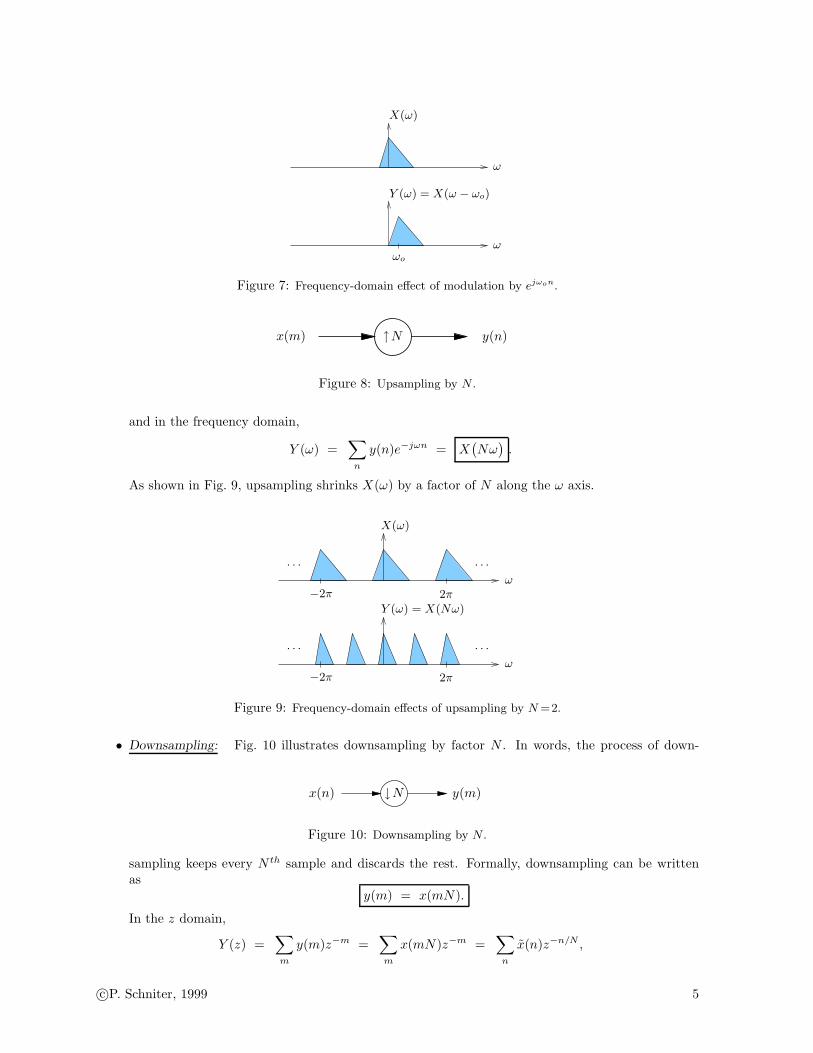
Note that X(ω − ωo) represents a shift of X(ω) up by ωo radians, as in Fig. 7.

• Upsampling: Fig. 8 illustrates upsampling by factor N . In words, upsampling means the insertionof N−1 zeros between every sample of the input process. Formally, upsampling can be expressedin the time domain as

y(n) =

{

x(n/N) when n = mN for m ∈ Z

0 else.

In the z-domain, upsampling causes

Y (z) =∑

n

y(n)z−n =∑

m

x(m)z−mN = X(zN)

,


X(ω)

Y (ω) = X(ω − ωo)

ωo

ω

ω

Figure 7: Frequency-domain effect of modulation by ejωon.

x(m) y(n)↑N

Figure 8: Upsampling by N .

and in the frequency domain,

Y (ω) =∑

n

y(n)e−jωn = X(Nω)

.

As shown in Fig. 9, upsampling shrinks X(ω) by a factor of N along the ω axis.

X(ω)

Y (ω) = X(Nω)

−2π

−2π 2π

2π

· · ·

· · ·

· · ·

· · ·

ω

ω

Figure 9: Frequency-domain effects of upsampling by N =2.

• Downsampling: Fig. 10 illustrates downsampling by factor N . In words, the process of down-

x(n) y(m)↓N

Figure 10: Downsampling by N .

sampling keeps every N th sample and discards the rest. Formally, downsampling can be writtenas

y(m) = x(mN).

In the z domain,

Y (z) =∑

m

y(m)z−m =∑

m

x(mN)z−m =∑

n

x̃(n)z−n/N ,


where

x̃(n) =

{

x(n) when n = mN for m ∈ Z

0 else.

The neat trick

1

N

N−1∑

p=0

ej 2πN

np =

{

1 when n = mN for m ∈ Z

0 else(1)

(which can be proven) allows us to rewrite x̃(n) in terms of x(n):

Y (z) =∑

n

x(n)

(

1

N

N−1∑

p=0

ej 2πN

np

)

z−n/N

=1

N

N−1∑

p=0

∑

n

x(n)(e−j 2π

Npz1/N

)−n

=1

N

N−1∑

p=0

X(e−j 2π

Npz1/N

).

Translating to the frequency domain,

Y (ω) =1

N

N−1∑

p=0

X

(ω − 2πp

N

)

.

As shown in Fig. 11, downsampling expands each 2π-periodic repetition of X(ω) by a factor of Nalong the ω axis. Note the spectral overlap due to downsampling, called “aliasing.”

X(ω)

X(ω/N)

Y (ω)

−4π

−4π

−4π

−2π

−2π

−2π

2π

2π

2π

4π

4π

4π

· · ·· · ·

· · ·· · ·

· · ·· · ·

ω

ω

ω

Figure 11: Frequency-domain effects of downsampling by N =2.

• Downsample-Upsample Cascade: Downsampling followed by upsampling (of equal factor N) isillustrated by Fig. 12. This structure is useful in understanding analysis/synthesis filterbanks thatlie at the heart of sub-band coding schemes. This operation is equivalent to zeroing all but themN th samples in the input sequence, i.e.,

y(n) =

{

x(n) when n = mN for m ∈ Z

0 else.


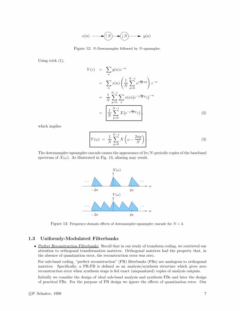
x(n) y(n)↓N↑N

Figure 12: N-Downsampler followed by N-upsampler.

Using trick (1),

Y (z) =∑

n

y(n)z−n

=∑

n

x(n)

(

1

N

N−1∑

p=0

ej 2πN

np

)

z−n

=1

N

N−1∑

p=0

∑

n

x(n)(e−j 2π

Npz)−n

=1

N

N−1∑

p=0

X(e−j 2π

Npz)

, (2)

which implies

Y (ω) =1

N

N−1∑

p=0

X

(

ω − 2πp

N

)

. (3)

The downsampler-upsampler cascade causes the appearance of 2π/N -periodic copies of the basebandspectrum of X(ω). As illustrated in Fig. 13, aliasing may result.

X(ω)

Y (ω)

−2π

−2π 2π

2π

· · ·

· · ·

· · ·

· · ·

ω

ω

Figure 13: Frequency-domain effects of downsampler-upsampler cascade for N = 2.

1.3 Uniformly-Modulated Filterbanks

• Perfect Reconstruction Filterbanks: Recall that in our study of transform coding, we restricted ourattention to orthogonal transformation matrices. Orthogonal matrices had the property that, inthe absence of quantization error, the reconstruction error was zero.

For sub-band coding, “perfect reconstruction” (PR) filterbanks (FBs) are analogous to orthogonalmatrices. Specifically, a PR-FB is defined as an analysis/synthesis structure which gives zeroreconstruction error when synthesis stage is fed exact (unquantized) copies of analysis outputs.

Initially we consider the design of ideal sub-band analysis and synthesis FBs and later the designof practical FBs. For the purpose of FB design we ignore the effects of quantization error. Our


rational is as follows: the absence of quantization error corresponds to the high bit-rate scenario,in which case we desire that the filtering operations inherent to sub-band coding introduce little orno error of their own. Removing the quantizers from Fig. 2, we obtain the analysis/synthesis FBsin Fig. 14.

+

......

x(n) u(n)

x0(n)

x1(n)

xN−1(n)

y0(n)

y1(n)

yN−1(n)

u0(n)

u1(n)

uN−1(n)

H0(z)

H1(z)

HN−1(z)

K0(z)

K1(z)

KN−1(z)↓N

↓N

↓N

↑N

↑N

↑N

Figure 14: N-band analysis and synthesis filterbanks.

• Uniform Modulation: The most conceptually straightforward FB is known as the “uniformlymodulated” FB. Uniform modulation means that all branches isolate signal components in non-overlapping frequency bands of equal width 2π/N . We will assume that the ith branch has itsfrequency band centered at ωi = 2iπ/N . (See Fig. 15.)

ω0 ω1 ω2 ω3

0 π 2π

2π/N ωi = 2πi/N

ω

Figure 15: Frequency bands for the uniformly-modulated filterbank (N = 4).

• Analysis FB: The ith frequency range may be isolated by modulating the input spectrum down byωi and lowpass filtering the result. (See the first two stages of the analysis bank in Fig. 17.) Theideal lowpass filter has linear phase and magnitude response that is unity for ω ∈ (−π/N, π/N) andzero elsewhere. (See Fig. 16.)

With ideal lowpass filtering, the resulting signals have (double-sided) bandwidths that are N timessmaller than the sampling rate. Nyquist’s sampling theorem [2] says that it is possible to samplesignals with this bandwidth at 1/N times the filter output rate without loss of information. Thissample rate change can implemented via downsampling-by-N , resulting in the analysis FB of Fig. 17.Note that the downsampling operation does not induce aliasing when the analysis filter is the ideallowpass filter described above.

• Synthesis FB: To reconstruct the input signal x(n), the synthesis FB must restore the downsampledsignals to their original sampling rate, re-modulate them to their original spectral locations, andcombine them.

Upsampling is the first stage of sampling-rate restoration. Recall from (3) (and Fig. 13) that adownsampler-upsampler cascade creates N −1 additional uniformly-spaced spectral copies of theoriginal baseband spectrum. Thus, to remove the unwanted spectral images, an “anti-imaging”


|H(ω)|

ω

π π−π/N π/N

Figure 16: Ideal (dashed) and typical (solid) prototype-filter magnitude responses for the uniformly modulatedfilterbank.

lowpass filter is applied to each upsampler’s output. Ideally, this lowpass filter is linear phase withmagnitude response that is unity for ω ∈ (−π/N, π/N) and zero elsewhere; the same specificationsgiven for the ideal analysis filter. (See Fig. 16.)

As shown in Fig. 17, re-modulation is accomplished by shifting the ith branch up by ωi.

When the analysis and synthesis filters share a common phase response, the re-modulator outputscan be combined coherently by a simple summation. Under all of these ideal conditions, the outputsignal u(n) is a potentially delayed (but otherwise perfect) copy of the input signal x(n):

u(n) = x(n − δ) for some delay δ.

+

×

×

×

×

×

×

......

x(n) u(n)

H(z)

H(z)

H(z)

K(z)

K(z)

K(z)↓N

↓N

↓N

↑N

↑N

↑N

e−jω0n

e−jω1n

e−jωN−1n

ejω0n

ejω1n

ejωN−1n

Figure 17: N-band modulated analysis/synthesis filterbanks.

• Effect of Non-Ideal Filtering: In practice, the analysis and synthesis filters will not have ideallowpass responses, and thus the reconstructed output u(n) will not necessarily equal a delayedversion of the input x(n). These shortcomings typically result from filter implementations based ona finite number of design parameters. (See Fig. 16 for a typical lowpass filter magnitude response.)

It should be noted that, under certain conditions, it is possible to design sets of analysis filters{Hi(z)} and synthesis filters {Ki(z)} with finite parameterizations which give the “perfect recon-struction” (PR) property [3]. Though such filters guarantee PR, they do not act as ideal bandpassfilters and thus do not accomplish perfect frequency analysis. (Consider the length-N DFT andDCT filter responses: by the orthogonal matrix argument, these are perfectly reconstructing, butfrom Figs. 4 and 5, they are far from perfect bandpass filters!)

Due to their limited frequency-selectivity, none of the currently-known PR filterbanks are appro-priate for high-quality audio applications. As a result, we focus on the design of filterbanks with


1. near -perfect reconstruction and

2. good frequency selectivity.

As we will see, it is possible to design practical filters with excellent frequency selectivity andresponses so close to PR that the smallest quantization errors swamp out errors caused by non-PRfiltering.

• Polyphase/DFT Implementation: When H(z) and K(z) are length-M FIR filters, the unique el-

ements in Fig. 17 are the N uniform-modulation coefficients {ej2πn/N ; n = 0, . . . , N−1} and the2M the lowpass filter coefficients {hn} and {kn}. It might not be surprising that each half of theuniformly-modulated FB has an implementation that requires only one N -dimensional DFT andM multiplies to process an N -block of input samples. Fig. 18 illustrates one such implementation,where the “polyphase” filters {H (`)(z)} and {K(`)(z)} are related to the “prototype” filters H(z)and K(z) through the impulse response relations:

h(`)m := hmN+`

k(`)m := kmN+`

for ` = 0, . . . , N − 1.

The term “polyphase” comes about because the magnitude responses of well-designed {H (`)(z)}and {K(`)(z)} are nearly flat, while the slopes of the phase response of these filters differ by smallamounts. The equivalence of Fig. 17 and Fig. 18 will be established in the homework.

......

......

+

+

z−1

z−1

z−1

z−1

z−1 z−1

ConjugateDFT:

√N W∗

N

ConjugateDFT:

√N W∗

N

x(n) u(n)H(0)(z)

H(1)(z)

H(N−1)(z)

K(0)(z)

K(1)(z)

K(N−1)(z)↓N

↓N

↓N

↑N

↑N

↑N

Figure 18: Polyphase/DFT implementation of N-band uniformly modulated analysis/synthesis filterbanks.

Recognize that the filter computations in Fig. 18 occur on downsampled (i.e., low-rate) data, incontrast to those in Fig. 17. To put it another way, all but one of every N filter outputs in Fig. 17are thrown away by the downsampler, whereas none of the filter outputs in Fig. 18 are thrown away.This reduces the number of required filter computations by a factor of N .

Additional computational reduction occurs when the DFT is implemented by a fast transform.Below we give a concrete example.

Example 1.1 (Computational Savings of Polyphase/FFT Implementation):Lets take a look at how many multiplications we save by using the polyphase/DFT analysis filterbank in Fig. 18instead of the standard modulated filterbank in Fig. 17. Here we assume that N is a power of 2, so that theDFT can be implemented with a radix-2 FFT.

With the standard structure in Fig. 17, modulation requires 2N real multiplies, and filtering of the complex-valued modulator outputs requires 2 × N × M additional real multiplies, for each input point x(n). This givesa total of

2N(M + 1) real multiplies per input.


In the polyphase/FFT structure of Fig. 18, it is more convenient to count the number of multiplies requiredfor each block of N inputs since each new N-block produces one new sample at every filter input and onenew N-vector at the DFT input. Since the polyphase filters are each length-M/N , filtering the block requiresN ×M/N = M real multiplies. Though the standard radix-2 N-dimensional complex-valued FFT uses N

2log2 N

complex multiplies, a real-valued N-dimensional FFT can be accomplished in N log2 N real multiplies when Nis a power of 2[4]. This gives a total of

M + N log2 N real multiplies per N inputs, or M/N + log2 N real multiplies per input!

Say we have N = 32 frequency bands and the prototype filter is length M = 512 (which turn out to be thevalues used in the MPEG sub-band filter). Then using the formulas above, the standard implementation requires

32832 multiplies per input, while the polyphase/DFT implementation requires only 21 !

1.4 MPEG Layers 1-3: Cosine-Modulated Filterbanks

• Though the uniformly modulated filterbank in Fig. 17 was shown to have the fast implementationin Fig. 18, the sub-band outputs are complex-valued for real-valued input, hence inconvenient (atfirst glance2) for sub-band coding of real-valued data.

In this section we propose a closely related filterbank with the following properties.

1. Real-valued sub-band outputs (assuming real-valued inputs),

2. Near-perfect reconstruction,

3. Polyphase/fast-transform implementation.

This turns out to be the filterbank specified in the MPEG-1 and 2 (layers 1-3) audio compressionstandards [1].

1.4.1 Filter Design

• Real-valued Sub-band Outputs: Recall the generic filterbank structure of Fig. 14. For the sub-band outputs to be real-valued (for real-valued input), we require that the impulse responses of{Hi(z)} and {Ki(z)} are real-valued. We can insure this by allocating the N (symmetric) frequencyband pairs shown in Fig. 19. The positive and negative halves of each band pair are centered at

ωi = (2i+1)π2N radians.

−ω0−ω1−ω2−ω3 ω0 ω1 ω2 ω3 π−π

π/Nωi = (2i+1)π

2N

ω

Figure 19: Frequency band pairs for the polyphase quadrature filterbank (N = 4).

We can consider each filter Hi(z) as some combination of symmetric positive-frequency and negative-frequency components

Hi(z) = aiFi(z) + biGi(z)

as shown in Fig. 20. When bi = a∗i and the pairs {Fi(z), Gi(z)} are modulated versions of the

2In the structure in Fig. 17, it would be reasonable to replace the standard DFT with a real-valued DFT (defined inthe notes on transform coding), requiring ≈ N log2 N real-multiplies when N is a power of 2. Though it is not clear tothe author why such a structure was not adopted in the MPEG standards, the cosine modulated filterbank derived in thissection has equivalent performance and, with its polyphase/DCT implementation, equivalent implementation cost.


−ωi ωi π−π

ω

π/Nπ/N

(2i+1)π/N

Hi(ω)

Fi(ω)Gi(ω)

Figure 20: Positive- and negative-frequency decomposition of Hi(ω). Note Ki(ω) will have a similar, if notidentical, frequency response.

same prototype filter H(z), we can show that Hi(z) must be real-valued:

Hi(z) = ai H(e−jπ 2i+12N z)

︸︷︷︸

Fi(z)

+ a∗i H(ejπ 2i+1

2N z)︸︷︷︸

Gi(z)

= ai

∑

n

hnejπ 2i+12N

nz−n + a∗i

∑

n

hne−jπ 2i+12N

nz−n

= Re(ai)∑

n

hnz−n(

ejπ 2i+12N

n + e−jπ 2i+12N

n)

+ jIm(ai)∑

n

hnz−n(

ejπ 2i+12N

n − e−jπ 2i+12N

n)

= Re(ai)∑

n

hnz−n · 2 cos

(

π2i+1

2Nn

)

+ jIm(ai)∑

n

hnz−n · 2j sin

(

π2i+1

2Nn

)

= 2∑

n

[

Re(ai) cos

(

π2i+1

2Nn

)

− Im(ai) sin

(

π2i+1

2Nn

)]

hnz−n (4)

• Aliasing Cancellation: Recall again the generic filterbank in Fig. 14. Here we determine conditionson real-valued {Hi(z)} and {Ki(z)} which lead to near-perfect reconstruction.

It will be insightful to derive an expression for the input to the ith reconstruction filter, {yi(n)}.The downsample-upsample-cascade equation (2) implies that

Yi(z) =1

N

N−1∑

p=0

Xi

(e−j 2π

Npz)

=1

N

N−1∑

p=0

Hi

(e−j 2π

Npz)X(e−j 2π

Npz)

=1

N

N−1∑

p=0

[

aiFi

(e−j 2π

Npz)

+ a∗i Gi

(e−j 2π

Npz)]

X(e−j 2π

Npz)

(5)

=1

N[aiFi(z) + a∗

i Gi(z)] X(z)︸︷︷︸

desired

+1

N

N−1∑

p=1

[

aiFi

(e−j 2π

Npz)

+ a∗i Gi

(e−j 2π

Npz)]

X(e−j 2π

Npz)

︸︷︷︸

undesired images

.

Thus the input to the ith reconstruction filter is corrupted by unwanted spectral images, and thereconstruction filter’s job is the removal of these images.

The reconstruction filter Ki(z) will have a bandpass frequency response similar (or identical) to thatof Hi(z) illustrated in Fig. 20. Due to the practical design considerations, neither Ki(z) nor Hi(z)


will be perfect bandpass filters, but we will assume that the only significant out-of-band energypassed by these filters will occur in the frequency range just outside of their passbands. (Note thelimited “spillover” in Fig. 20.)

Under these assumptions, the only undesired images in Yi(ω) that will not be completely attenuatedby Ki(ω) are the images adjacent to Fi(ω) and Gi(ω). Which indices p in (5) are responsible forthese adjacent images? Equation (5) implies that index p = ` shifts the frequency response upby 2π`/N radians. Since the passband centers of Fi(z) and Gi(z) are (2i + 1)π/N radians apart,

the passband of Gi

(e−j 2π

Npz)

will reside directly to the left of the passband of Fi(z) when p = i.

Similarly, the passband of Gi

(e−j 2π

Npz)

will reside directly to the right of the passband of Fi(z) when

p = i + 1. See Fig. 21 for an illustration. Using the same reasoning, the passband of Fi

(e−j 2π

Npz)

will reside directly to the right of the passband of Gi(z) when p = −i and directly to the left whenp = −(i + 1). The only exceptions to this rule occur when i = 0, in which case the images to theright of Gi(z) and to the left of Fi(z) are desired, and when i = N − 1, in which case the images tothe left of Gi(z) and to the right of Fi(z) are desired.

−ωi ωi π−π

ω

p = −(i+1) p = −i p = i p = i+1

Fi(z)Gi(z)

Fi

`

e−j 2πN

pz´

Fi

`

e−j 2πN

pz´

Gi

`

e−j 2πN

pz´

Gi

`

e−j 2πN

pz´

Figure 21: Spectral images of Yi(ω) not completely attenuated by Ki(ω).

Based on the arguments above, we can write {ui(n)}, the output of the ith reconstruction filter, asfollows:

Ui(z) = Ki(z)Yi(z)

=1

NKi(z)

[aiFi(z)X(z) + a∗

i Gi(z)X(z)]

︸︷︷︸

desired

+1

NKi(z)

[

aiFi

(ej 2π

Niz)X(ej 2π

Niz)+ a∗

i Gi

(e−j 2π

Niz)X(e−j 2π

Niz)]

︸︷︷︸

aliasing from inner undesired images when 1 ≤ i ≤ N − 1

+1

NKi(z)

[

aiFi

(ej 2π

N(i+1)z

)X(ej 2π

N(i+1)z

)+ a∗

i Gi

(e−j 2π

N(i+1)z

)X(e−j 2π

N(i+1)z

)]

︸︷︷︸

aliasing from outer undesired images when 0 ≤ i ≤ N − 2

.(6)

The previous equation shows that Ui(z) is corrupted by the portions of the undesired images notcompletely removed by the reconstruction filter Ki(z). In the filterbank context, this undesiredbehavior is referred to as aliasing. But notice that aliasing contributions to the signal U(z) =∑

i Ui(z) will vanish if the inner aliasing components in Ui(z) cancel the outer aliasing componentsin Ui−1(z). This happens when

Ki(z)[

aiFi

(ej 2π

Niz)X(ej 2π

Niz)

+ a∗i Gi

(e−j 2π

Niz)X(e−j 2π

Niz)]

= −Ki−1(z)[

ai−1Fi−1

(ej 2π

Niz)X(ej 2π

Niz)

+ a∗i−1Gi−1

(e−j 2π

Niz)X(e−j 2π

Niz)]

.


which occurs under satisfaction of the two conditions below.

aiKi(z)Fi

(ej 2π

Niz)

= −ai−1Ki−1(z)Fi−1

(ej 2π

Niz)

(7)

a∗i Ki(z)Gi

(e−j 2π

Niz)

= −a∗i−1Ki−1(z)Gi−1

(e−j 2π

Niz). (8)

We assume from this point on that the real-valued filters {Hi(z)} and {Ki(z)} are constructedusing modulated versions of a lowpass prototype filter H(z). (This assumption is required for theexistence of a polyphase filterbank implementation.)

Hi(z) = aiFi(z) + a∗i Gi(z)

Ki(z) = ciFi(z) + c∗i Gi(z)where

{

Fi(z) = H(e−j π

2N(2i+1)z

)

Gi(z) = H(ej π

2N(2i+1)z

)

Then condition (7) becomes

aiciH(e−j π

2N(2i+1)z

)H(ej π

2N(2i−1)z

)+ aic

∗i H(ej π

2N(2i+1)z

)H(ej π

2N(2i−1)z

)

= −ai−1ci−1H(e−j π

2N(2i−1)z

)H(ej π

2N(2i+1)z

)− ai−1c

∗i−1H

(ej π

2N(2i−1)z

)H(ej π

2N(2i+1)z

). (9)

Lets take a closer look at the products H(e−j π

2N(2i+1)z

)H(ej π

2N(2i−1)z

)in the previous equation.

As illustrated in Fig. 22, these products equal zero when 1 ≤ i ≤ N/2 since their passbands do notoverlap. Setting these products to zero in (9) yields the condition

aic∗i = − ai−1c

∗i−1 for 1 ≤ i ≤ N − 1 , (10)

which can also be shown to satisfy (8).

− π

2N(2i−1) π

2N(2i+1)π

2N(2i+1) − 2π

π−πω

· · ·· · ·

(2(N−i)−1)π/N (2i−1)π/N

H`

ej π2N

(2i−1)z´

H`

e−j π2N

(2i+1)z´

H`

e−j π2N

(2i+1)z´

Figure 22: Illustration of vanishing terms in (9).

Next we concern ourselves with the requirements on a0 and c0. Assuming (10) is satisfied, we knowthat inner aliasing in Ui(z) cancels outer aliasing in Ui−1(z) for 1 ≤ i ≤ N − 1. Hence, from (6)and (9),

U(z) =

N−1∑

i=0

Ui(z)

=1

N

N−1∑

i=0

Ki(z)Hi(z)X(z)

=1

N

N−1∑

i=0

[

ciH(e−j π

2N(2i+1)z

)+ c∗i H

(ej π

2N(2i+1)z

)]

·[

aiH(e−j π

2N(2i+1)z

)+ a∗

i H(ej π

2N(2i+1)z

)]

X(z)


Noting that the passbands of H(e−j π

2N(2i+1)z

)and H

(ej π

2N(2i+1)z

)do not overlap for 1 ≤ i ≤ N−2,

we have

U(z) =1

N

[

(a0c∗0 + a∗

0c0)H(e−j π

2N z)H(ej π

2N z)

+ (aN−1c∗N−1 + a∗

N−1cN−1)H(e−j π

2N(2N−1)z

)H(ej π

2N(2N−1)z

)

+N−1∑

i=0

(

aiciH2(e−j π

2N(2i+1)z

)+ a∗

i c∗i H

2(ej π

2N(2i+1)z

))]

X(z). (11)

The first two terms in (11) represent aliasing components that prevent flat overall response at ω = 0and ω = π, respectively. These aliasing terms vanish when

a0c∗0 = −a∗

0c0

aN−1c∗N−1 = −a∗

N−1cN−1(12)

What remains is

U(z) =1

N

N−1∑

i=0

(

aiciH2(e−j π

2N(2i+1)z

)+ a∗

i c∗i H

2(ej π

2N(2i+1)z

))

X(z).

• Phase Distortion: Perfect reconstruction requires that the analysis/synthesis system has no phasedistortion. To guarantee the absence of phase distortion, we require that the composite system

Q(z) :=U(z)

X(z)=

1

N

N−1∑

i=0

aiciH2(e−j π

2N(2i+1)z

)+ a∗

i c∗i H

2(ej π

2N(2i+1)z

)

has a linear phase response. (Recall that a linear phase response is equivalent to a pure delay inthe time domain.) This linear-phase constraint will provide the final condition used to specify theconstants {ai} and {ci}.We start by examining the impulse response of Q(z). Using a technique analogous to (4), we canwrite

Q(z) =2

N

2M−2∑

n=0

(N−1∑

i=0

Re(aici) cos

(

π2i+1

2Nn

)

− Im(aici) sin

(

π2i+1

2Nn

))(∑

k

hkhn−k

)

z−n

Above, we have used the property that multiplication in the z-domain implies convolution in thetime domain.

For Q(z) to be linear phase, it’s impulse response must be symmetric. Let us assume that theprototype filter H(z) is linear phase, so that {hn} is symmetric. Thus

∑

k hmhn−k is symmetricabout n = M − 1, and thus for linear phase Q(z), we require that the quantity

N−1∑

i=0

Re(aici) cos

(

π2i+1

2Nn

)

− Im(aici) sin

(

π2i+1

2Nn

)

is symmetric about n = M − 1, i.e.,

N−1∑

i=0

Re(aici) cos

(

π2i+1

2N(M − 1 + n)

)

− Im(aici) sin

(

π2i+1

2N(M − 1 + n)

)

=

N−1∑

i=0

Re(aici) cos

(

π2i+1

2N(M − 1 − n)

)

− Im(aici) sin

(

π2i+1

2N(M − 1 − n)

)


for n = 0, . . . , M − 1. Using trigonometric identities, it can be shown that the condition above isequivalent to

0 =

N−1∑

i=0

sin

(

π2i+1

2Nn

)[

Re(aici) sin

(

π2i+1

2N(M − 1)

)

+ Im(aici) cos

(

π2i+1

2N(M − 1)

)]

,

which is satisfied when

Im(aici)

Re(aici)= − sin

(π 2i+1

2N (M − 1))

cos(π 2i+1

2N (M − 1)) = tan

(

−π2i+1

2N(M − 1)

)

.

Restricting |ai| = |ci| = 1, the previous equation requires that

aici = e−jπ 2i+12N

(M−1) . (13)

It can be easily verified that the following {ai} and {ci} satisfy conditions (10), (12), and (13):

ai = e−jπ M+N−14N

(2i+1)

ci = e−jπ M−N−14N

(2i+1).(14)

Plugging these into the expression for Hi(z) we find that

Hi(z) = aiH(e−jπ 2i+1

2N z)

+ a∗i H(ejπ 2i+1

2N z)

=

M−1∑

n=0

(

aiejπ 2i+1

2Nn + a∗

i e−jπ 2i+1

2Nn)

hnz−n

=M−1∑

n=0

(

ejπ 2i+12N

(n−M+N−12 ) + e−jπ 2i+1

2N(n−M+N−1

2 ))

hnz−n

=

M−1∑

n=0

2 cos(π 2i+1

2N

(n − M+N−1

2

))hn

︸︷︷︸

impulse response of Hi(z)

z−n. (15)

Repeating this procedure for Ki(z) yields

Ki(z) =

M−1∑

n=0

2 cos(π 2i+1

2N

(n − M−N−1

2

))hn

︸︷︷︸

impulse response of Ki(z)

z−n. (16)

At this point we make a few comments on the design of the lowpass prototype H(z). The perfectH(z) would be an ideal linear-phase lowpass filter with cutoff at ω = π/2N , as illustrated in Fig. 23.Such a filter would perfectly separate the subbands as well as yield flat composite magnituderesponse, as per (13). Unfortunately, however, this perfect filter is not realizable with a finitenumber of filter coefficients. So, what we really want is a finite-length FIR filter having goodfrequency selectivity, nearly-flat composite response, and linear phase. The length-512 prototypefilter specified in the MPEG standards is such a filter, as evidenced by the responses in Fig. 24.Unfortunately, the standards do not describe how this filter was designed, and a thorough discussionof multirate filter design is outside the scope of this course. For more on prototype filter design, wepoint the interested reader to [3, p. 358] and [5].

To conclude, (15) and (16) give impulse response expressions for a set of real-valued filters that com-prise a near-perfectly reconstructing filterbank (under suitable selection of {hi}). This is commonlyreferred to3 as a “cosine-modulated filterbank” because all filters are based on cosine modulations

3The MPEG standards refer to this filterbank as a “polyphase quadrature” filterbank (PQF), the name given to thetechnique by an early technical paper [6].


|H(ω)|

ω

π π−π/2N π/2N

Figure 23: Ideal (dashed) and typical (solid) prototype-filter magnitude responses for the cosine-modulatedfilterbank. Note bandwidth relative to Fig. 16.

0 0.5 1 1.5 2 2.5 3−120

−100

−80

−60

−40

−20

0

20prototype filter

radians

mag

nitu

de [d

B]

0 0.5 1 1.5 2 2.5 3−2

0

2

4

6

8x 10

−4 composite system

radians

mag

nitu

de [d

B]

Figure 24: Magnitude response of |H(ω)| of MPEG prototype filter and the resulting composite response |Q(ω)|,where N = 32 and M = 16N = 512.

of a real-valued linear-phase lowpass prototype H(z). The near-perfect reconstruction propertyfollows from the frequency-domain cancellation of adjacent-spectrum aliasing and the lack of phasedistortion.

It should be noted that our derivation of the cosine modulated filterbank is similar to that in [6]except for the treatments of phase distortion. See Chapter 8 of [3] for a more comprehensive viewof cosine-modulated filterbanks.

• Polyphase Implementations: Recall the uniformly modulated filterbank in Fig. 17, whose combined

modulator-filter coefficients can be constructed using products of the terms hn and ej πN

in. Fig. 18shows a computationally-efficient polyphase/DFT implementation of the analysis filter which re-quires only M multiplies and one N -dimensional DFT computation for calculation of N subbandoutputs. We might wonder: Is there a similar polyphase/fast-transform implementation of thecosine-modulated filterbank derived in this section?

From (15), we see that the impulse responses of {Hi(z)} are products of the terms hn andcos(π 2i+1

2N

(n − M+N−1

2

))for n = 0, . . . , M − 1. Note that the inverse-DCT matrix Ct

n can be


specified via components with form similar to the cosine term in (15):

[Ct

N

]

i,n=

√

2

Nαn cos

(

π(2i + 1)

2Nn

)

; i, n = 0 . . . N−1.

for α0 = 1/√

2, αn6=0 = 1.

Thus it may not be surprising that there exist polyphase/DCT implementations of the cosine-modulated filterbank. Indeed, one such implementation is specified in the MPEG-2 audio compres-sion standard [1]. This particular implementation is the focus of the next section.

1.4.2 MPEG Filterbank Implementation

• Since MPEG audio compression standards are so well-known and widespread, a detailed look atthe MPEG filterbank implementation is warranted. The cosine-modulated, or polyphase-quadraturefilterbank described in the previous section is used in MPEG Layers 1-3. (The MPEG hierarchywill be described in a later chapter.) This section discusses the specific implementation suggestedby the MPEG-2 standard [1].

• The MPEG standard specifies 512 prototype filter coefficients, the first of which is zero. To adaptthe MPEG filter to our cosine-modulated-filterbank framework, we append a zero-valued 513th

coefficient so that the resulting MPEG prototype filter becomes symmetric and hence linear phase.Since the standard specifies N = 32 frequency bands, we have

M = 513 = 16N + 1.

Plugging this value of M into the filter expressions (15) and (16), the 2π-periodicity of the cosineimplies that they may be rewritten as follows.

Hi(z) =16N−1∑

n=0

2 cos(π 2i+1

2N

(n − N

2

))hn

︸︷︷︸

impulse response of Hi(z)

z−n

Ki(z) =16N−1∑

n=0

2 cos(π 2i+1

2N

(n + N

2

))hn

︸︷︷︸

impulse response of Ki(z)

z−n.

• Encoding: Here we derive the encoder filterbank implementation suggested in the MPEG-2 standard

[1]. Using xi(n) to denote the output of the ith analysis filter, we have

xi(n) =

16N−1∑

k=0

[

2 cos(

π 2i+12N

(

k − N2

))

hk

]

x(n − k).

The relationship between xi(n) and its downsampled version si(m) is given by

si(m) = xi(mN),

so that the downsampled analysis output si(m) can be written as

si(m) =

16N−1∑

n=0

[

2 cos(

π 2i+12N

(

n − N2

))

hn

]

x(mN − n).

Using the substitution n = kN + ` for 0 ≤ ` ≤ N−1,

si(m) = 2

15∑

k=0

N−1∑

`=0

cos(π 2i+1

2N

(kN + ` − N

2

))

︸︷︷︸

repeats every 4 increments of k

sign changes every 2 increments of k

hkN+` x((m − k)N − `

)

=

15∑

k=0

N−1∑

`=0

cos(π 2i+1

2N

(〈k〉2N + ` − N

2

))

︸︷︷︸

repeats every 2 increments of k

2 (−1)bk/2chkN+`︸︷︷︸

analysis window

x((m − k)N − `

)


Fig. 25 illustrates this process.

· · ·

· · ·

· · ·

· · ·

· · ·· · ·

...

...

↓ ∗ ↓ ∗

↓ ∗ ↓ ∗

↓ ∗

↓ ∗

↓ ∗

↓ ∗

↓ ∗

↓ ∗

↓ ∗

↓ ∗

↓ =↓ =↓ =↓ =

+++

k = 0 k = 1 k = 2 k = 3 k = 4 k = 15

x`

mN´

, . . . x`

(m−1)N´

, . . . x`

(m−2)N´

, . . . x`

(m−3)N´

, . . . x`

(m−4)N´

, . . . . . . , x`

(m−16)N + 1´

h0, . . . , hN−1 hN , . . . , h2N−1 h2N , . . . , h3N−1 h3N , . . . , h4N−1 h4N , . . . , h5N−1 h15N , . . . , h16N−1

2, 2, 2, . . . , 2, 2, 2 2, 2, 2, . . . . . . , −2, −2, −2. . . , −2, −2, −2

0

0 N

2N

2N 3N 4N

4N

5N 15N

16N

16N

j = 0 j = 1 j = 2N−1

i = 0

i = 1

i = N−1

s0(m)

s1(m)

sN−1(m)

cosine matrix transformation:

cos(π 2i+1

2N

(j − N

2

))

Figure 25: MPEG encoder filterbank implementation suggested in [1].

• Decoding: Here we derive the dencoder filterbank implementation suggested in the MPEG-2 stan-

dard [1]. Using yi(n) to denote the output of the ith upsampler,

ui(n) =

16N−1∑

k=0

[2 cos

(π 2i+1

2N

(k + N

2

))hk

]yi(n − k).

The input to the upsampler si(m) is related to the output yi(n) by

yi(n) =

{

si(n/N) when n/N ∈ Z

0 else,

so that

ui(n) =∑

{k: n−kN

∈Z}

[2 cos

(π 2i+1

2N

(k + N

2

))hk

]si

(n−kN

).


Lets write n = mN + ` for 0 ≤ ` ≤ N−1 and k = pN + q for 0 ≤ q ≤ N−1. Then due to therestricted ranges of ` and q,

n − k

N= m − p +

` − q

N∈ Z ⇒ ` = q.

Using these substitutions in the previous equation for ui(n),

ui(mN + `) = 2

15∑

p=0

cos(π 2i+1

2N

(pN + ` + N

2

))hpN+` si(m − p).

Summing ui(mN + `) over i to create u(mN + `),

u(mN + `) = 2

N−1∑

i=0

15∑

p=0

cos(π 2i+1

2N

(pN + ` + N

2

)))

︸︷︷︸

repeats every 4 increments of p

sign changes every 2 increments of p

hpN+` si(m − p)

=

15∑

p=0

2 (−1)bp/2chpN+`︸︷︷︸

synthesis window

N−1∑

i=0

cos(π 2i+1

2N

(〈p〉2N + ` + N

2

)))

︸︷︷︸

=

8

>

<

>

:

cos(π 2i+1

2N

(` + N

2

))p even

cos(π 2i+1

2N

(` + N + N

2

))p odd

si(m − p)

If we define

vj(m) =N−1∑

i=0

cos(π 2i+1

2N

(j + N

2

))si(m) for 0 ≤ j ≤ 2N − 1,

(note the range of j !) then we can rewrite

u(mN + `) =∑

p=0,2,...,14

(−1)bp/2chpN+` v`(m − p) +∑

p=1,3,...,15

(−1)bp/2chpN+` v`+N (m − p).

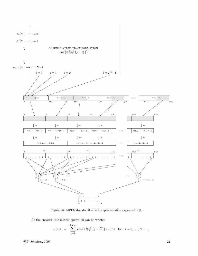
Fig. 26 illustrates the construction of u(mN + `) using the notation

v(m) =(v0(m) · · · v2N−1(m)

).

• DCT Implementation of Cosine Matrixing: As seen in Fig. 25 and Fig. 26, the filterbank implemen-tations suggested by the MPEG standard require a cosine matrix operation that, if implementedusing straightforward arithmetic, requires 32 × 64 = 2048 multiply/adds at both the encoder anddecoder. Note, however, that the cosine transformations in Fig. 25 and Fig. 26 do bear a great dealof similarity to the DCT:

yk =

√

2

Nαk

N−1∑

n=0

xn cos(π 2n+1

2N k); k = 0 . . .N−1, (17)

for α0 = 1/√

2, αk 6=0 = 1,

xn =

√

2

N

N−1∑

k=0

αk yk cos(π 2n+1

2N k); n = 0 . . .N−1, (18)

which we know has a fast algorithm: Lee’s 32×32 fast-DCT, for example, requires only 80 multipli-cations and 209 additions [7]. So how do we implement the matrix operation using the fast-DCT?A technique has been described clearly in [8], the results of which are summarized below.


· · ·

· · ·

· · ·

· · ·

· · ·

· · ·

...

...

↓ ∗

↓ ∗

↓ ∗

↓ ∗

↓ ∗

↓ ∗

↓ ∗

↓ ∗

↓ ∗

↓ ∗

↓ = ↓ =↓ =

+++

s0(m)

s1(m)

sN−1(m)

i = 0

i = 1

i = N−1

j = 0 j = 1 j = 2 j = 2N−1


cos(π 2i+1

2N

(j + N

2

))

v(m) v(m−1) v(m−2) v(m−3) v(m−15)

h0, . . . , hN−1 hN , . . . , h2N−1 h2N , . . . , h3N−1 h3N , . . . , h4N−1 h15N , . . . , h16N−1

2, 2, 2, . . . , 2, 2, 2 . . . , −2, −2, −2−2, −2, −2, . . . , −2, −2, −2

0

0

0

0

N

N

2N

2N

2N

3N

4N

4N

4N

6N 8N

15N

15N 16N

16N

30N 32N

u(mN) u(mN+1) u(mN+N−1)

Figure 26: MPEG decoder filterbank implementation suggested in [1].

At the encoder, the matrix operation can be written

si(m) =

2N−1∑

j=0

cos(π 2i+1

2N

(j − N

2

))wj(m) for i = 0, . . . , N − 1,


where {w0(m), . . . , w2N−1(m) is created from {x(m), . . . , x(m− 16N + 1)} by windowing, shifting,and adding. (See Fig. 25.) It is shown in [8] that we can write

si(m) =N−1∑

j=0

cos(π 2i+1

2N j)w̄j(m); i = 0, . . . , N − 1, (19)

where, for N = 32, {w̄j(m)} is the following manipulation of {wj(m)}:

w̄j(m) :=

w16(m) j = 0

w16+j(m) + w16−j(m) j = 1, 2, . . . , 16

w16+j(m) − w80−j(m) j = 17, 18, . . . , 31.

Compare (19) to the inverse DCT in (18).

At the decoder, the matrix operation can be written

vj(m) =

N−1∑

i=0

cos(π 2i+1

2N

(j + N

2

))si(m) for j = 0, . . . , 2N − 1,

where {v0(m), . . . , v2N−1(m)} are windowed, shifted, and added to compute {u(m)}. (See Fig. 26.)It is shown in [8] that, for N = 32, {vj(m)} can be calculated by first computing {v̄j(m)}:

v̄j(m) =

N−1∑

i=0

cos(π 2i+1

2N j)si(m); j = 0, . . . , N − 1 (20)

and rearranging the outputs according to

vj(m) :=

v̄j+16(m) j = 0, 1, . . . , 15,

0 j = 16,

−v̄48−j(m) j = 17, 18, . . . , 47,

−v̄j−48(m) j = 48, 49, . . . , 63.

Compare (20) to the DCT in (17).

2 MDCT Filterbanks

• Hybrid Filter Banks: In more advanced audio coders such as MPEG “Layer-3” or MPEG “Ad-vanced Audio Coding” (the details of which will be discussed later), the 32-band polyphase quadra-ture filterbank (PQF) is thought to not give adequate frequency resolution, and so an additionalstage of frequency division is cascaded onto the output of the PQF. This additional frequencydivision is accomplished using the so-called “Modified DCT” (MDCT) filterbank. (See Fig. 27.)

• Lapped Transforms: The MDCT is a so-called “lapped transform.” At the encoder, blocks oflength 2Q which overlap by Q samples are windowed and transformed, generating Q subbandsamples each. At the decoder, the Q subband samples are inverse-transformed and windowed. Thewindowed output samples are overlapped with and added to the previous Q windowed outputs toform the output stream. Fig. 28 gives an intuitive view of the coding/decoding operation, whileFig. 29 and Fig. 30 specify the specific coder/decoder implementations used in the MPEG schemes.

• Perfect Reconstruction: Based on the cancellation of time-domain aliasing components, [9] and[10] show that the MDCT acheives perfect-reconstruction when window {wn} is chosen so thatoverlapped squared copies sum to one, i.e.,

1 = w2n+Q + w2

n for 0 ≤ n ≤ Q − 1.


N-bandPolyphase Quadrature

Filterbank

MDCT

MDCT

MDCT

...

}

Q-bands

}

Q-bands

}

Q-bands

Figure 27: Hybrid filterbank scheme used in MPEG Layer-3 (where N = 32 and Q switches bewteen 6 and 18)and MPEG AAC (where N = 4 and Q switches between 128 and 1024).

overlapping input windows windowed and overlapped outputs

transforminverse

transform

Figure 28: A lapped transform.

The “sine” window

wn = sin

(π

2Qn

)

for 0 ≤ n ≤ 2Q − 1

is one example of a window satisfying this requirement, and it turns out to be the one used inMPEG Layer-3.

• Frequency Resolution: With a window length that is only twice the number of transform outputs,we cannot expect very good frequency selectivity. But, it turns out that this is not a problem. InMPEG Layer-3, sine-window MDCTs appear at the outputs of a 32-band PQF where frequencyselectivity is not a critical issue due to the limited frequency resolution of the human ear. In MPEGAAC, a 4-band PQF in conjunction with an optimized MDCT window function gives frequencyselectivity just above that which current psychoacoustic models deem necessary [11].

• Window Switching: Larger values of Q lead to increased frequency resolution but decreased timeresolution. Time resolution is linked to the following: error due to the quantization of one MDCToutput is spread out over ≈ 2QN time-domain output samples. For signals of a transient nature,choosing QN too high leads to audible “pre-echoes.” For less transient signals, on the other hand,the same value of QN might not be perceptible (and the increased frequency resolution might be


x(mQ−2Q+1) x(mQ−2Q+2) x(mQ)

w(0) w(1) w(2Q − 1)· · ·· · ·

· · ·· · ·

↓ ∗

↓=

j = 0 j = 1 j = 2Q − 1 i = 0

i = 1

i = Q − 1


cos(

π 2i+12Q (j + no)

)

Figure 29: MDCT filterbank: encoder implementation.


cos(

π 2i+12Q (j + no)

)

j = 0 j = 1 j = 2Q − 1

i = 0

i = 1

i = Q − 1

w(0) · · · w(2Q−1)

· · ·∗ ∗∗

↓=

+ ++

um(0) · · · um(Q−1) um(Q) · · · um(2Q−1) um−1(0) · · · um−1(Q−1) um−1(Q) · · · um−1(2Q−1)

u(mQ) u(mQ+1) u(mQ+Q−1)

Figure 30: MDCT filterbank: decoder implementation.

very beneficial). Hence, most advanced coding schemes have a provision to switch between different


time/frequency resolutions depending on local signal behavior.

In MPEG Layer-3, for example, Q switches between 6 and 18. This is accomplished using a sinewindow of length 36, a sine window of length 12, and intermediate windows which are used to switchbetween the long and short windows while retaining the perfect reconstruction property. Fig. 31shows an example window sequence.

Figure 31: Example MDCT window sequence for MPEG Layer-3.

References

[1] ISO/IEC 13818-3, “Information Technology–Generic Coding of Moving Pictures and AssociatedAudio Information, Part 3: Audio,” 1998.

[2] A.V. Oppenheim and R.W. Schafer, Discrete-Time Signal Processing, Englewood Cliffs, NJ:Prentice-Hall, 1989.

[3] P.P. Vaidyanathan, Multirate Systems and Filter Banks, Englewood Cliffs, NJ: Prentice-Hall, 1993.

[4] H.V. Sorensen, D.L. Jones, M.T. Heideman, and C.S. Burrus, “Real-valued fast Fourier transformalgorithms,” IEEE Transactions on Acoustics, Speech, and Signal Processing, vol. 35, pp. ??, June,1987.

[5] R.E. Crochiere and L.R. Rabiner, Multirate Digital Processing, Englewood Cliffs, NJ: Prentice-Hall,1983.

[6] J.H. Rothweiler, “Polyphase quadrature filters—A new subband coding technique,” in Proc. IEEE

International Conference on Acoustics, Speech, and Signal Processing (Boston, MA), pp. 1280-3,1983.

[7] B.G. Lee, “A new algorithm to compute the discrete cosine transform,” IEEE Transactions on

Acoustics, Speech, and Signal Processing, vol. 32, no. 6, pp. 1243-5, Dec. 1984.

[8] K. Konstantinides, “Fast subband filtering in MPEG audio coding,” IEEE Signal Processing Letters,vol. 1, no. 2, pp. 26-8, Feb. 1994.

[9] J.P. Princen, A.W. Johnson, and A.B. Bradley, “Subband/transform coding using filter bank designsbased on time domain aliasing cancellation,” in Proc. IEEE International Conference on Acoustics,

Speech, and Signal Processing (??), pp. 2161-4, 1987.

[10] J.P. Princen and A.B. Bradley, “Analysis/synthesis filter bank design based on time domain aliasingcancellation,” IEEE Transactions on Acoustics, Speech, and Signal Processing, vol. 34, no. 5, pp.1153-61, Oct. 1986.

[11] M. Bosi, et al., “ISO/IEC MPEG-2 Advanced Audio Coding,” Journal of the Audio Engineering

Society, vol. 45, no. 10, pp. 789-812, Oct. 1997.


Documents

EE-597 Class Notes – Sub-Band Codingschniter/ee597/handouts/subband_coding.pdf · EE-597 Class Notes – Sub-Band Coding Phil Schniter June 11, 2004 1 Sub-Band Coding 1.1 Introduction