Notes 7

MATH 337, by T. Lakoba, University of Vermont 69

7 The shooting method for solving BVPs

7.1 The idea of the shooting method

In the first four subsections of this lecture we will only consider BVPs that satisfy the conditionsof Theorems 6.1 or 6.2 and thus are guaranteed to have a unique solution.

Suppose we want to solve a BVP with Dirichlet boundary conditions:

y′′ = f(x, y, y′), y(a) = α, y(b) = β . (7.1)

We can rewrite this BVP in the form:

y′ = zz′ = f(x, y, z)y(a) = αy(b) = β .

(7.2)

The BVP (7.2) will turn into an IVP if we replace the boundary condition at x = b with thecondition

z(a) = θ , (7.3)

where θ is some number. Then we can solve the resulting IVP by any method that we havestudied in Lecture 5, and obtain the value of its solution y(b) at x = b. If y(b) = β, then wehave solved the BVP. Mostly likely, however, we will find that after the first try, y(b) 6= β.Then we should choose another value for θ and try again. There is actually a strategy of howthe values of θ need to be chosen. This strategy is simpler for linear BVPs, so this is the casewe consider next.

7.2 Shooting method for the Dirichlet problem of linear BVPs

Thus, our immediate goal is to solve the linear BVP

y′′ + P (x)y′ + Q(x)y = R(x) with Q(x) ≤ 0, y(a) = α, y(b) = β . (7.4)

To this end, consider two auxiliary IVPs:

u′′ + Pu′ + Qu = R,

u(a) = α, u′(a) = 0(7.5)

andv′′ + Pv′ + Qv = 0,

v(a) = 0, v′(a) = 1 ,(7.6)

where we omit the arguments of P (x) etc. as this should cause no confusion. Next, considerthe function

w = u + θv, θ = const . (7.7)

Using Eqs. (7.5) and (7.6), it is easy to see that

(u + θv)′′ + P (u + θv)′ + Q (u + θv) = R,

(u + θv)(a) = α, (u + θv)′(a) = θ ,(7.8)


i.e. w satisfies the IVPw′′ + Pw′ + Qw = R,

w(a) = α, w′(a) = θ .(7.9)

Note that the only difference between (7.9) and (7.4) is that in (7.9), we know the value of w′

at x = a but do not know whether w(b) = β. If we can choose θ in such a way that w(b) doesequal b, this will mean that we have solved the BVP (7.4).

To determine such a value of θ, we first solve the IVPs (7.5) and (7.6) by an appropriatemethod of Lecture 5 and find the coresponding values u(b) and v(b). We then choose the valueθ = θ0 by requiring that the corresponding w(b) = β, i.e.

w(b) = u(b) + θ0v(b) = β . (7.10)

This w(x) is the solution of the BVP (7.4), because it satisfies the same ODE and the sameboundary conditions at x = a and x = b; see Eqs. (7.9) and (7.10). Equation (7.10) yields thefollowing equation for the θ0:

θ0 =β − u(b)

v(b). (7.11)

Thus, solving only two IVPs (7.5) and (7.6) and constructing the new function w(x) ac-cording to (7.7) and (7.11), we obtain the solution to the linear BVP (7.4).

Consistency check: In (7.4), we have required that Q(x) ≤ 0, which guarantees that aunique solution of that BVP exists. What would have happened if we had overlooked to imposethat requirement? Then, according to Theorem 6.2, we could have run into a situation wherethe BVP would have had no solutions. This would occur if

v(b) = 0 . (7.12)

But then Eqs. (7.6) and (7.12) would mean that the homogeneous BVP

v′′ + Pv′ + Qv = 0,

v(a) = 0, v(b) = 0 ,(7.13)

must have a nontrivial16 solution. The above considerations agree, as they should, with theAlternative Principle for the BVPs, namely: the BVP (7.4) may have no solutions if thecorresponding homogeneous BVP (7.13) has nontrivial solutions.

7.3 Generalizations of the shooting method for linear BVPs

If the BVP has boundary conditions other than of the Dirichlet type, we will still proceedexactly as we did above. For example, suppose we need to solve the BVP

y′′ + Py′ + Qy = R,

y(a) = α, y′(b) = β,(7.14)

which has the Neumann boundary condition at the right end point. Denote y1 = y, y2 = y′,and rewrite this BVP as

y′1 = y2

y′2 = −Py2 −Qy1 + R

y1(a) = α, y2(b) = β .

(7.15)

16Indeed, since we also know that v′(a) = 1, then v(x) cannot identically equal zero on [a, b].


Using the vector/matrix notations with

~y =

(y1

y2

),

we can further rewrite this BVP as

~y ′ =(

0 1−Q −P

)~y +

(0R

),

y1(a) = α

y2(b) = β .(7.16)

Now, in analogy with Eqs. (7.5) and (7.6), consider two auxiliary IVPs:

~u ′ =(

0 1−Q −P

)~u +

(0R

), ~u(a) =

(α

0

); (7.17)

~v ′ =(

0 1−Q −P

)~v , ~v(a) =

(0

1

). (7.18)

Solve these IVPs by an appropriate method and obtain the values ~u(b) and ~v(b). Next, considerthe vector

~w = ~u + θ~v, θ = const. (7.19)

Using Eqs. (7.17)–(7.19), it is easy to see that this new vector satisfies the IVP

~w ′ =(

0 1−Q −P

)~w +

(0R

), ~w(a) =

(α

θ

). (7.20)

At x = b, its value is

~w(b) =

(u1(b) + θv1(b)

u2(b) + θv2(b)

), (7.21)

where u1 is the first component of ~u etc. From the last equation in (7.16), it follows that weare to require that

w2(b) = β . (7.22)

Equations (7.21) and (7.22) together yield

u2(b) + θv2(b) = β , ⇒ (7.23)

θ0 =β − u2(b)

v2(b). (7.24)

Thus, the vector ~w given by Eq. (7.19) where ~u, ~v, and θ satisfy Eqs. (7.17), (7.18), and(7.24), respectively, is the solution of the BVP (7.16).

Also, the shooting method can be used with IVPs of order higher than the second. Forexample, consider the BVP

x3y′′′ + xy′ − y = −3 + ln x ,

y(a) = α, y′(b) = β, y′′(b) = γ .(7.25)

As in the previous example, denote y1 = y, y2 = y′, y3 = y′′ and rewrite the BVP (7.25) in thematrix form:

~y ′ = A~y +~r ,

y1(a) = α

y2(b) = β

y3(b) = γ .

(7.26)


where

~y =

y1

y2

y3

, A =

0 1 0

0 0 11x3 − 1

x2 0

, ~r =

00

−3+ln xx3

.

Consider now three auxiliary IVPs:

~u ′ = A~u +~r ,

~u(a) =

α00

;

~v ′ = A~v ,

~v(a) =

010

;

~w ′ = A~w ,

~w(a) =

001

.

(7.27)

Solve them and obtain ~u(b), ~v(b), and ~w(b). Then, construct ~z = ~u + θ~v + φ~w, where θ and φ

are numbers which will be determined shortly. At x = b, one has

~z(b) =

. . .

u2(b) + θv2(b) + φw2(b)

u3(b) + θv3(b) + φw3(b)

. (7.28)

If we require that ~z satisfy the BVP (7.26), we must have

~z(b) =

. . .

β

γ

. (7.29)

From Eqs. (7.28) and (7.29) we form a system of two linear equations for the unknown coeffi-cients θ and φ:

θv2(b) + φw2(b) = β − u2(b) ,

θv3(b) + φw3(b) = γ − u3(b) .(7.30)

Solving this linear system, we obtain values θ0 and φ0 such that the corresponding ~z = ~u +θ0~v + φ0~w solves the BVP (7.26) and hence the original BVP (7.25).

7.4 Caveat with the shooting method, and its remedy, the multipleshooting method

Here we will encounter a situation where the shooting method in its form described above doesnot work. We will also provide a way to modify the method so that it would be usable again.

Let us consider the BVP

y′′ = 302 (y − 1 + 2x) ,

y(0) = 1, y(b) = 1− 2b ; b > 0.(7.31)

Its exact solution isy = 1− 2x ; (7.32)

by Theorem 6.2 this solution is unique. Note that the general solution of only the ODE (withoutboundary conditions) in (7.31) is

y = 1− 2x + Ae30x + B e−30x . (7.33)


Now let us try to use the shooting method to solve the BVP (7.31). Following the lines ofSec. 7.2, we set up auxiliary IVPs

u′′ = 302(u− 1 + 2x) ,

u(0) = 1, u′(0) = 0 ;

v′′ = 302v ,

v(0) = 0, v′(0) = 1 ;(7.34)

and solve them. The exact solutions of (7.34) are:

u = 1− 2x +1

30

(e30x − e−30x

), v =

1

60

(e30x − e−30x

). (7.35)

Then Eq. (7.11) provides the value of the auxiliary parameter θ0:

θ0 =(1− 2b)− (1− 2 · b + 1

30(e30·b − e−30·b) )

160

(e30·b − e−30·b)= −2 . (7.36)

That is,u(7.35) + (−2) · v(7.35) = 1− 2x = exact solution , (7.37a)

or, in detail:

{1− 2x +

1

30

(e30x − e−30x

)}+ (−2) ·

{1

60

(e30x − e−30x

)}= 1− 2x. (7.37b)

Note that each of the terms in curly brackets in (7.37b) is a very large number. For example,for x = 1.4, the magnitude of the second term is:

1

30

(e30·1.4 − e−30·1.4

) ≈ 1

30· e30·1.4 ≈ 5.8 · 1016 . (7.38)

Now recall that Matlab’s round-off error eps = 2.2 · 10−16. This means two things:(i) if for some numbers x and y, one has x− y < eps, then Matlab “thinks” that x− y = 0;(ii) if z is such a large number that z > 1/eps, then Matlab may compute it with an errorthat may be of order 1 and even larger.(In one of the QSA’s you will be asked to verify these statements.)

Statement (ii) above along with (7.38) meanthat the expression on the l.h.s. of (7.37b) forx ≈ 1.4 is evaluated by Matlab with an er-ror of order 1 or larger. That is, the l.h.s. of(7.37b), as it is evaluated by Matlab, deviatesfrom the exact solution by as much — or more— than the exact solution itself. This quali-tatively explains the origin of the “burst” seennear x = 1.4 in the figure on the right, wherethe numerical solution of (7.31) with b = 1.4 isshown. 0 0.2 0.4 0.6 0.8 1 1.2 1.4

0

10

20

30

40

50

60

x

y

exact

numerical

A reason why this burst is so large — almost two orders of magnitude greater than theexact solution, while the “pieces” u(x) and v(x) in (7.37) are only a factor of 2–3 greater than1/ eps, — is not quite clear. Perhaps, one explanation can be that the global errors of thenumerical solutions for u(x) and v(x) are proportional to the large number e30x (see Eq. (1.16)


in Lecture 1), and such large errors for u(x) and v(x) do not completely cancel out in (7.37).Another reason can be that the parameter θ0 in (7.36) may be evaluated by Matlab with around-off error: θ0 = −2 + eps, and then the computed solution is

y = u(7.35) + (−2 + eps) · v(7.35) = 1− 2x +eps

60

(e30x − e−30x

). (7.39)

Again, the third term in that expression may be of order 1 or greater.

The way in which the shooting method is to be modified in order to handle the above problemis suggested by the figure on the previous page. Namely, one can see that the numerical solutionis quite accurate up to the vicinity of the right end point, where x ≈ 1.4 and where the factore30x multiplied by some small error, overtakes the exact solution. Therefore, if we split theinterval [0, 1.4] into two adjoint subintervals, [0, 0.7] and [0.7, 1.4], and perform shooting oneach of these subintervals, then the corresponding exponential factor, e30·0.7 ∼ 109, will be wellresolved by Matlab: e30·0.7 ∼ 109 ¿ 1 /eps ∼ 5 · 1015.

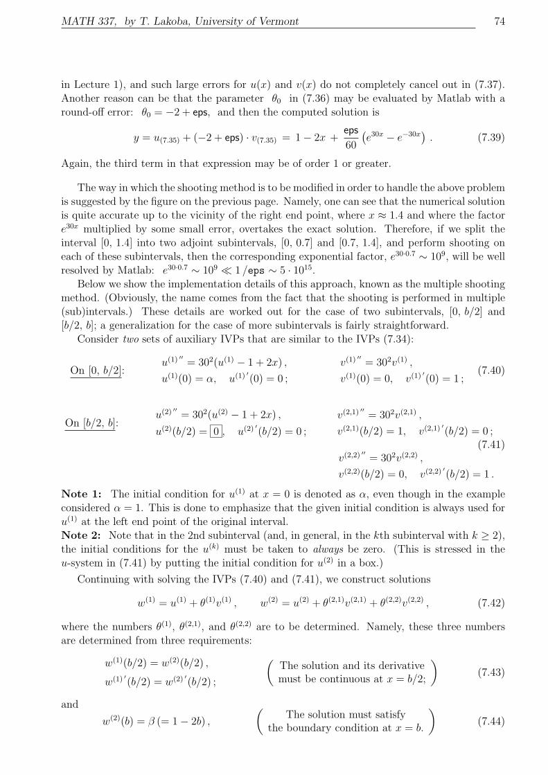
Below we show the implementation details of this approach, known as the multiple shootingmethod. (Obviously, the name comes from the fact that the shooting is performed in multiple(sub)intervals.) These details are worked out for the case of two subintervals, [0, b/2] and[b/2, b]; a generalization for the case of more subintervals is fairly straightforward.

Consider two sets of auxiliary IVPs that are similar to the IVPs (7.34):

On [0, b/2]:u(1) ′′ = 302(u(1) − 1 + 2x) ,

u(1)(0) = α, u(1) ′(0) = 0 ;

v(1) ′′ = 302v(1) ,

v(1)(0) = 0, v(1) ′(0) = 1 ;(7.40)

On [b/2, b]:u(2) ′′ = 302(u(2) − 1 + 2x) ,

u(2)(b/2) = 0 , u(2) ′(b/2) = 0 ;

v(2,1) ′′ = 302v(2,1) ,

v(2,1)(b/2) = 1, v(2,1) ′(b/2) = 0 ;(7.41)

v(2,2) ′′ = 302v(2,2) ,

v(2,2)(b/2) = 0, v(2,2) ′(b/2) = 1 .

Note 1: The initial condition for u(1) at x = 0 is denoted as α, even though in the exampleconsidered α = 1. This is done to emphasize that the given initial condition is always used foru(1) at the left end point of the original interval.Note 2: Note that in the 2nd subinterval (and, in general, in the kth subinterval with k ≥ 2),the initial conditions for the u(k) must be taken to always be zero. (This is stressed in theu-system in (7.41) by putting the initial condition for u(2) in a box.)

Continuing with solving the IVPs (7.40) and (7.41), we construct solutions

w(1) = u(1) + θ(1)v(1) , w(2) = u(2) + θ(2,1)v(2,1) + θ(2,2)v(2,2) , (7.42)

where the numbers θ(1), θ(2,1), and θ(2,2) are to be determined. Namely, these three numbersare determined from three requirements:

w(1)(b/2) = w(2)(b/2) ,

w(1) ′(b/2) = w(2) ′(b/2) ;

(The solution and its derivativemust be continuous at x = b/2;

)(7.43)

and

w(2)(b) = β (= 1− 2b) ,

(The solution must satisfy

the boundary condition at x = b.

)(7.44)


Equations (7.43) and (7.44) yield:

w(1)(b/2) = w(2)(b/2) ⇒ u(1)(b/2) + θ(1)v(1)(b/2) = 0 + θ(2,1) · 1 + θ(2,2) · 0 ;

w(1) ′(b/2) = w(2) ′(b/2) ⇒ u(1) ′(b/2) + θ(1)v(1) ′(b/2) = 0 + θ(2,1) · 0 + θ(2,2) · 1 ;

w(2)(b) = β ⇒ u(2)(b) + θ(2,1) · v(2,1)(b) + θ(2,2) · v(2,2)(b) = β .(7.45)

In writing out the r.h.s.’s of the first two equations above, we have used the boundary conditionsof the IVP (7.41).

The three equations (7.45) form a linear system for the three unknowns θ(1), θ(2,1), andθ(2,2). (Recall that u(1)(b/2) etc. are known from solving the IVPs (7.40) and (7.41).) Thus,finding the θ(1), θ(2,1), and θ(2,2) from (7.45) and substituting them back into (7.42), we obtainthe solution to the original BVP (7.31).

Important note: The multiple shooting method, at least in the above form, can onlybe used for linear BVPs, because it is only for them that the linear superposition principle,allowing us to write

w = u + θv ,

can be used.

Further reading on the multiple shooting method can be found in:• P. Deuflhard, “Recent advances in multiple shooting techniques,” in Computation techniquesfor ODEs, I. Gladwell and D.K. Sayers, eds. (Academic Press, 1980);• J. Stoer and R. Burlish, “Introduction to numerical analysis” (Springer Verlag, 1980);• G. Hall and J.M. Watt, “Modern numerical methods for ODEs” (Clarendon Press, 1976).

7.5 Shooting method for nonlinear BVPs

As has just been noted above, for nonlinear BVPs, the linear superposition of the auxiliarysolutions u and v cannot be used. However, one can still proceed with using the shootingmethod by following the general guidelines of Sec. 7.1.

As an example, let us consider the BVP

y′′ =y2

2 + x,

y(0) = 1, y(2) = 1 .

(7.46)

We again consider the auxiliary IVP

y′1 = y2 ,

y′2 =y2

1

2 + x;

y1(0) = 1, y2(0) = θ .

(7.47)


The idea is now to find the right value(s) of θ iter-atively. To motivate the iteration algorithm, let usactually solve the IVP (7.47) for an (equidistant)set of θ’s inside some large interval and look at theresult, which is shown in the figure on the right.(The reason this particular interval of θ valuesis chosen is simply because the instructor knowswhat the result should be.) This figure shows thatthe boundary condition at the right end point,

y(2)|as the function of θ = 1 , (7.48)

can be considered as a nonlinear algebraic equationwith respect to θ. Correspondingly, we can employwell-known methods of solving nonlinear algebraicequations for solving nonlinear BVPs.

−15 −10 −5 0 −5

−3

−1

1

3

θ

y(2

)

prescribed boundary value

θ θ

Probably the simplest such a method is the secant method. Below we will show how to useit to find the values θ̄ and ¯̄θ, for which y(2) = 1 (see the figure). Suppose we have tried twovalues, θ1 and θ2, and found the corresponding values y(2)|θ1 and y(2)|θ2 . Denote

F (θk) = y(2)|θk− 1 , k = 1, 2 . (7.49)

Thus, our goal is to find the roots of the equation

F (θ) = 0 . (7.50)

Given the first two values of F (θ) at θ = θ1,2, the secant method proceeds as follows:

θk+1 = θk − F (θk)[F (θk)−F (θk−1)

θk−θk−1

] , and then compute F (θk+1) from (7.49). (7.51)

The iterations are stopped when |F (θk+1) − F (θk)| becomes less than a prescribed tolerance.In this manner, one will find the values θ̄ and ¯̄θ and hence the corresponding two solutions ofthe nonlinear BVP (7.46). You will be asked to do so in a homework problem.

7.6 Broader applicability of the shooting method

We will conclude with two remarks. The first will outline another case where the shootingmethod can be used. The other will mention an important case where this method cannot beused.

7.6.1 Shooting method for finding discrete eigenvalues

Consider a BVP

y′′ + (2sech2x− λ2)y = 0, x ∈ (−∞,∞), y(|x| → ∞) → 0 . (7.52)


Here the term 2sech2x could be generalized to any“potential” V (x) that has one or several “humps”in its central region and decays to zero as |x| → ∞.Such a BVP is solvable (i.e., a y(x) can be foundsuch that y(|x| → ∞) → 0) only for some specialvalues of λ, called the eigenvalues of this BVP. Thecorresponding solution, called an eigenfunction, isa localized “blob”, which has some “structure” inthe region where the potential is significantly dif-ferent from zero and which vanishes at the ends ofthe infinite line. An example of such an eigenfunc-tion is shown on the right. Note that in general, aneigenfunction may have a more complicated struc-ture at the center than just a single “hump”.

−10 0 100

x

y

A variant of the shooting method which can find these eigenvalues is the following. First,since one cannot literally model the infinite line interval (−∞,∞), consider the above BVP onthe interval [−R, R] for some reasonably large R (say, R = 10). For a given λ in the BVP,choose the initial conditions for the shooting as

y(−R) = y0, y′(−R) = λ · y(−R), (7.53)

for some very small y0 which we will discuss later. The reason behind the above relation betweeny′(−R) and y(−R) is this. Since the potential 2sech2x (almost) vanishes at |x| = R, then(7.52) reduces to y′′−λ2y ≈ 0, and hence y′ ≈ λy at x = −R. Note that of the two possibilitiesy′ ≈ λy and y′ ≈ −λy which are implied by y′′ − λ2y ≈ 0, we have chosen the former, becauseit is its solution,

y = eλx, (7.54)

which agrees with the behavior of the eigenfunction at the left end of the real line (see thefigure above).

The constant y0 in (7.53) can be taken as

y0 = e−c R, (7.55)

where the constant c is of order one. Often one can simply take c = 1.Now, compute the solution of the IVP consisting of the ODE in (7.52) and the initial

condition (7.53) and record the value y(R). This value can be denoted as G(λ) since it hasbeen obtained for a particular value of λ: G(λ) ≡ y(R)|λ. Repeat this process for values ofλ = λmin + j∆λ, j = 0, 1, 2, . . . in some specified interval [λmin, λmax]; as a result, one obtainsa set of points representing a curve G(λ). Those values of λ where this curve crosses zerocorrespond to the eigenvalues17. Indeed, there y(R) = 0, which is the approximate relationsatisfied by eigenfunctions of (7.52) at x = R for R À 1.

17In practice, one uses a more accurate method, but the description of this technical detail is outside thescope of this lecture.


7.6.2 Inapplicability of the shooting method in higher dimensions

Boundary value problems considered in this section are one-dimensional, in that they involvethe derivative with respect to only one variable x. Such BVPs often arise in description ofone-dimensional objects such as beams and strings. A natural generalization of these to twodimensions are plates and membranes. For example, a classic Helmholtz equation

∂2u

∂x2+

∂2u

∂y2+ k2u = 0, (7.56)

where u = 0 along the boundaries of a square with vertices (x, y) = (0, 0), (1, 0), (1, 1), (0, 1),arises in the mathematical description of oscillations of a square membrane.

One could attempt to obtain a solution of this BVP by shooting from, say, the left sideof this square to the right side. However, not only is this tedious to implement while ac-counting for all possible combinations of ∂u/∂x along the side (x = 0, 0 ≤ y ≤ 1), butalso results of such shooting will be dominated by numerical error and will have nothing incommon with the true solution. The reason is that any IVP for certain two-dimensional equa-tions, of which (7.56) is a particular case, are ill-posed. We will not go further into thisissue18 since it would substantially rely on the material studied in a course on partial dif-ferential equations. What is important to remember out of this brief discussion is that theshooting method can be used only for one-dimensional BVPs.

In the next lecture we will introduce alternative methods that can be used to solve BVPsboth in one and many dimensions. However, we will only consider their applications in onedimension.

7.7 Questions for self-assessment

1. Explain the basic idea behind the shooting method (Sec. 7.1).

2. Why did we require that Q(x) ≤ 0 in (7.4)?

3. Verify (7.8).

4. Suppose that Q(x) > 0, and we have found that v(b) = 0, as in (7.12). Does this meanonly that the BVP (7.4) will have no solutions, or are there other possibilities?

5. Let Q(x) > 0, as in the previous question, but now we have found that v(b) 6= 0. Whatpossibilities for the number of solutions to the BVP do we have?

6. Verify (7.15) and (7.16).

7. Verify (7.20).

8. Verify (7.26).

9. Suppose you need to solve a 5th-order linear BVP. How many auxiliary systems do youneed to consider? How many parameters (analogues of θ) do you need to introduce andthen solve for?

18We will, however, arrive at the same conclusion, but from another view point, in Lecture 11.


10. What allows us to say that by Theorem 6.2 the solution (7.32) is unique?

11. Verify (7.36) and (7.37).

12. Verify statements (i) and (ii) found below Eq. (7.38). Specifically, do the following.(i) Enter in Matlab an expression 2+k*eps where k is some number. Observe howMatlab’s output changes as k increases from being less than 1 to being greater than 1.(ii) Enter into Matlab an expression 2.5/eps - (2.5/eps + 1) and note the result.Vary the coefficient 2.5 (simultaneously in both terms) and, separately, the coefficient 1and observe what happens.

13. What is a likely cause of the large deviation of the numerical solution from the exact onein the figure found below Eq. (7.38)?

14. Describe the key idea behind the multiple shooting method.

15. Suppose we use 3 subintervals for multiple shooting. How many parameters analogous toθ(1), θ(2,1), and θ(2,2) will we need? What are the meanings of the conditions from whichthese parameters can be determined?

16. Verify that the r.h.s.’es in (7.45) are correct.

17. Describe the key idea behind the shooting method for nonlinear BVPs.

18. For a general nonlinear BVP, can one tell how many solutions one will find?

Documents

Notes 7