.- !L”

I.

Sensor and Simulation Notes

Note 264c~::~:~

19 June 1979 FOR FWLK RELEASE

p$@#9 5A7/9~Interaction Between a Para+lel-Plate EMPSimulator and a Cylindrical Test Object

.TohnLam

Dikewood Industries, Inc.Albuquerque, New Mexico “87106

Abstract

The interaction between a bounded-wave EMP simulator and a test

object is studied with a geometrical model. The model consists of a

finite, open-ended cylinder inside a parallel-plate waveguide. The inter-

action problem is formulated exactly by means of an integrodifferential

equation, which is subsequently reduced to a matrix equation. An approxi-

mate analytical solution of the matrix equation is obtained. The singular-

ities of the solution in the complex-frequency plane are investigated. The

effects of the simulatorftest-object interaction on the pole singularities

are numerically evaluated.

.

Sensor and Simulation Notes

Note 264

19 June 1979

Interaction Between a Parallel-Plate EMPSimulator and a Cylindrical Test Object

John Lam

Dikewood Industries, Inc.Albuquerque, New Mexico 87106

Abstract

The interaction between a bounded-wave EMP simulator and a test

object is studied with a geometrical

finite, open-ended cylinder inside a

action problem is formulated exactly

model. The model consists of a

parallel-plate waveguide. The inter-

by means of an integrodifferential

equation, which is subsequently reduced to a matrix equation. An approxi-

mate analytical solution of the matrix equation is obtained. The singular-

ities of the solution in the complex-frequency plane are investigated. The

effects of the simulator/test-object interaction on the pole singularities

are numerically evaluated.

geometrical models, cylindricalelectromagnetic pulse simulators

bodies, frequency, parallel–plate waveguides,

. .

Section

I

11

Iv

v

VII

INTRODUCTION

ELECTROMAGNETIC POTEN’HALS

DERIVATION OF INTEGRODIFFERENTIAL EQUATION

REDUCTION TO MATRIX EQUATION

APPROXIMATE ANALYTICAL SOLUTION

COMPLEX-FREQUENCY-PLLVE SINGULARITIES

NUMERICAL RESULTS

CONCLUS1ONS

REFERENCES

APPENDIX

10

19

26

35

36

38

——

ILLUSTRATIONS

Figure

1 Geometry of the Interaction Between a

and a Cylindrical Test Object

Page

Parallel-Plate Simulator

5

2 Branch-Cut Singularities in the Complex-Frequency Plane

Characterizing the Wave~uide Modes 20

3 Pole Singularities in the

4 Pole Singularities in the

5 Pole Singularities in the

Complex-Frequency Plane for L/h=0.2 30

Complex-Frequency Plane for L/h=O.5003 31

Complex-Frequency Plane for L/h=O.8003 32

TABLES

Table w

1 Pole Singularity Parameters for L/h = 0.2 27

2 Pole Singularity Parameters for L/h = 0.5003 28

3 Pole Singularity Parameters for L/h = 0.8003 29

—

.

SECTION I

INTRODUCTION

Bounded-wave electromagnetic-pulse (EMP) simulators provide one means to

generate simulated EMP’s for testing the EMP responses of aircraft and missiles

on the system level (ref. 1). A simulator can be designed to launch an electro-

magnetic pulse into the simulator volume which closely approximates the actual

nuclear Eli I?.This ability, however, does not imply that the actual interaction

between the nuclear FM? and the test object is also thereby automatically closely

simulated. In the simulator there exists an additional interaction between the

simulator structure and the test object which is absent in the actual EMP

encounter in free space. This interaction adversely affects the quality of

the simulation. In order to interpret and utilize correctly the simulator

test data, it is necessary to estimate and make allowance for this sinmlator/

test-object interaction.

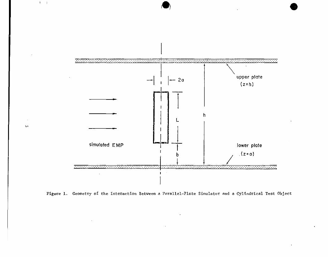
This report presents an analytical study of the simulatorftest-object

interaction. It employs an idealized model with simplified geometries to keep

the mathematics manageable. The bounded-wave E?tPsimulator is modeled by a

pair of parallel, perfectly conducting, flat plates of infinite extent, as

depicted in figure 1. Such a structure is an electromagnetic waveguide. Let

the spacing between the two plates be denoted by h . A rectangular coordinate

system can be set up such that the lower plate is at Z=o and the upper plate

at z=h . The test object is taken to be a hollow cylinder or tube of cross-

sectional radius a and length L . It is considered to be perfectly conducting

and of infinitesimal thickness. The axis of the tube is oriented perpendicular

to the two plates, and can be taken to coincide with the z-axis. The length

L is then of necessity less than h . Let the,lower end of the tube be at a

height b above the lower plate.

The tube is a sufficiently simple model of a missile or aircraft structure,

while the infinite plates constitute an idealization of the parallel-plate

section of a bounded-wave simulator. By choosing this idealized model, it is

possible to perform a rigorous and exact formulation of the simulator/test-

object interaction problem which is at the same time not too complicated for an

analytical solution.

-1 I

—. ,,, . . . . . . . . . . . . . . . . . . . . . . . . . . . . . . . . . . . ................................................... . . . . . . . .......... ........ . . . . . . . . . . . . . . . ... ..

I1’1I + 20

m

simulated E I$lp

t

I

I

-’kI

L

I

T

t b

1

:...:.:.:..,....:...:.......:...,...........................................

\upper plate

(z=h)

h

lower plate

/’

.(Z=O)

I

I

Figure 1. Geometry of the Interaction Between a Psrallel-Plate Simulator and a Cylindrical Test Object

SECTION 11

ELECTROMAGNETIC POTENTIALS

The specific goal of this analysis is to calculate the electric current

induced on the cylinder when the parallel-plate waveguide is excited by an

electromagnetic wave, This electromagnetic wave can, for example, be a simul-

ated EMP in the form of the transverse-electromagnetic (TEN) mode of the

waveguide. The effect of the simulator/test-object interaction is estimated

by

is

in

comparing this induced current with its corresponding value when the cylinder

excited in free space in the absence of the simulator.

The current induced on the cylinder by an incident electromagnetic wave

the parallel-plate waveguide can be evaluated by solving an integro-

differential equation. The derivation of this equation requires a considerable

amount of calculation. One first introduces the electromagnetic scalar and

vector potentials V and ~ for the electromagnetic fields Esc and Rsc— —

scattered off the cylinder and the plates, such that

E_sc(+ = - vv(~,t) -~~(~,t) , ~sc(~,t) =VxA(r,t) (1)——

In the Lorentz gauge these potentials are related by the Lorentz condition:

V*A(r,t) + ~~v(~,t) = o—— C2 at(2)

and individually satisfy the wave equation:

At z~O and h, on the surfaces of the two parallel plates, the

tangential components of ES= and the normal component of Bsc must vanish.—

By writing out equations (1) and (2) in rectangular component form, one can

easily convince oneself that these boundary conditions on the fields imply

t?~efollowing boundary conditions on the potmtials:

6

V(~,t) = Ax(~,t) = A+t) = o

-

(4)

for ~=o and h . Thus the scalar potential and the tangential components

the vector potential satisfy the homogeneous Dirichlet boundary condition on

the plates, while the normal component of the vector potential satisfies the

homogeneous Neumann boundary condition.

of

It will be convenient to go over from the time variable t to a complex

frequency variable s by introducing the Laplace transforms of all time-

dependent quantities. For example, the Laplace transform of the scalar

potential is

\

a

V(g,s) = dt e-stv(&,t)

-e

(5)

Under this transformation equations (3) become

(vz-yz)v(~,s) = o , (v2-y2)~(~,s) = o (6)

where

Y=: (7)

Their solutions can be represented as definite integrals over the surface of

the cylinder:

v(~,s) =+~

GD@_’,s)u(~’ ,s)dS’o

\GD(r,r’,s)Kx(~’,s)dS’Ax(~,s) = U __

o

Ay(r,s) = P./GD(r,r’,s)Ky(~’,s)ds’— ——

(8)

7

In these expressions, u and K are the surface charge and current densities

induced on the cylinder by the incident wave;‘D

and G?4

are the Creents

functions for the Dirichlet and Neumann boundary-value problems of the parallel-

plate waveguide; and the field position vector r = (x,y,z) stands for a point—in space while the source position vector rl = (x’,y’,z’) stands for a point—on the surface of the cylinder.

The Green~s functions CD and GN are solutions of the nonhomogeneous

Helmholtz equation:

(V2-y2)GD(r,r;,s) =- _ _63(r-r7)——

(V2-y2)GN(r,r’,s) = - &3{r- r’)—— ——

{9)

They satisfy, respectively, the homogeneous Dirichlet boundary condition GD=O

and the homogeneous Neumann boundary condition aGN/az = ~ on the plates z=O

and h . In addition they both satisfy the outgoing-wave condition at infinity.

Using standard Green;s function techniques, one finds that

w

CD(~,~’,s) = ~ Un(x,y,x’,y’,s)sfn pnz sin pnz’n=l

~(r,r’,s) = ~ Un(X,Y,X’,Y’,S)COS p z COS P .’——n=O n n

with

==Pn h

and

Un(x,y,x’,y’,s) .+lt~~.)n

Here K. is a modified Bessel function,

~.

and Cn is defined by:

J(X-X’)2+ (y-y’)z

I2 n=O

c=n

1 n=l,2,3, ,..

{13)

(14)

8

(11)

(12)

Furthermore, to satfsfy the outgoing-wave condition, the branch of the square

root in equation (12) is to be chosen to make

/ Y*+P: +y

as y+co .

(15)

—

—

.

SECTION 111

DERIVATION OF INTEGRODIFFERENTIAL EQUATION

The surface charge density u can be eliminated from the calculation by

using the continuity equation:

su(r,s) -i-V*K(r,s) = O—— (16)

The independent unknown quantities of the problem are then the two components

of the surface current density ~ . One can set up two integrodiffereritial

equations for ~ by applying the boundary conditions on the tangential compo-

nents of the total electric field on the surface of the cyl%nder. In a standard

cylindrical coordinate system (p,~,z) with polar axis coinciding with the axis

of the cylinder, these boundary conditions are

for r on the cylfnder.—

(17)

The two integrodifferential equations so derived are generally coupled.

However, for the specific geometry of this problem, it is possible to obtain

from them a single closed integrodifferential equation for the total axial

current I defined as

1211

I(z,s) = a d~ Kz(Y,z,s)

o

(18)

The total axial current by itself is often sufficient to characterize the

excitation of a thin cylinder at low frequencies, since in this limit the

circumferential current fs small by comparison.

To derive the integrodifferential equation for the total axial current I ,

one writes down the first of the boundary conditions (17) in terms of the

potentials:

~v(~,s) + s Az(tjs) “ E:c(~,s) (19)

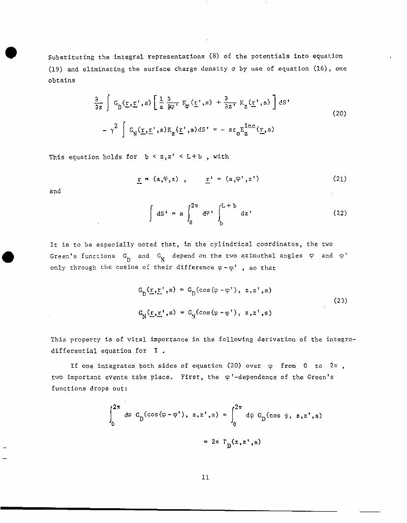
Substituting the integral representations (8) of the potentials into equation

(19) and eliminating the surface charge density u by use of equation (16), one

obtains

a

I [

la aGD(r,r’,s) :~1$(~’,s) +~Kz(Y’,s)

5 –– 1d~t

-Y*!GN(L~l’>s)Kz(~’,s)dS’ = - se Einc(~,s)

Oz

This equation holds for b ~ Z,Z’ < L+b , with

(20)

r = (a,~,z) , ~’ = (a,T’,z’)

and

1 [21T

(

L+bdS’ = a w’ dz ,

It is to be especially

Green’s functions‘E

.I Jo

noted that, in the

and G~ depend on~

Jb

(21)

(22)

cylindrical coordinates, the two

the two azimuthal angles T and q’

only through the cosine of their difference y -T’ , so that

GD(~,~’,s) = $-+os(c+D++’), 2,2’,S)

(23)

GN(~,~’,s) = GN(cos(cp-(#), Z,Z’,s)

This property is of vital importance in the following derivation of the integro-

differential equation for I .

If one integrates both sides of equation (20) over q from O to 2i7,

two important events take place. First, the q’ -dependence of the Green’s

functions drops out:

/

211

J

*7Ido GD(cos(Wp’), 2,2’,s) = d$ GD(cOS $, Z,z’,s)

o 0

—

—

= 2~ rD(z,z’,s)

11

(2X

/

21rd?% (COS(ql-~$), Z,ZJ,S) = d~ GN(COS $, 2,2’,S)

o 0

= 2n rN(z,z’,s) (24)

Therefore the subsequent O’-integration in equation (20) is carried out solely

on the surface current density components ~ and Kz . Second, the term in

%vanishes after the cp’-integration because

~

2Z yl=2Tr

df#*K& ,s) ‘KY(+s) =0o q~=o

On the other hand the ~’-integration of Kz yields directly

current I , as defined in equation (18). Gathering together

one obtains the following nonhomogeneous integro-differential

(25)

the total axial

all these results,

equation for I :

a L+b

I dz’rD(z,z’,s)a

z— 1(2’,s)az’

(26)

z L+b

-YI

dz’rN(z,z’,s)I(z’,s) = - SEOE$C(Z,S)

b

where

I2m

*=(Z,S) =+ do E~c(a,q?,z,s)

o

(27)

~incThat is, z is the average

field around the circumference

One should emphasize that

mation has been invoked in its

is actually made possible through the judicious choice of the geometry of the

model. If a different geometry were chosen, it is doubtful that a closed

equation for I similar to equation (26) could be derived without the help

of assumptions and approximations.

value of the z-component of the incident electric

of the cylinder at a fixed value of z .

equation (26) is an exact equation. No approxi-

deri.vation. This remarkable, rigorous result

12

The two functions ‘Dand

‘Nin equation (26) can be evaluated

explicitly in closed form. Substituting equation (10) into equation (24)

one obtains

rD(z,z’,s) = ~ W (s)sin pnz sin pnz’n.l n

I’N(Z,ZJ,S)= y w {S)cos p z Cos p z’n*=() n n

\

21T

wn(S) = & d@--?rhc

.0 (2a~ sin $)

=~~o(~a)~o(~a)

n

(28)

where

(29)

—

Use has been made of the addition theorem for the cylindrical functions (ref. 2)

in evaluating the integral in equation (29).

13

SECTION IV

REI)UCTIONTO MATRIX EQUATION

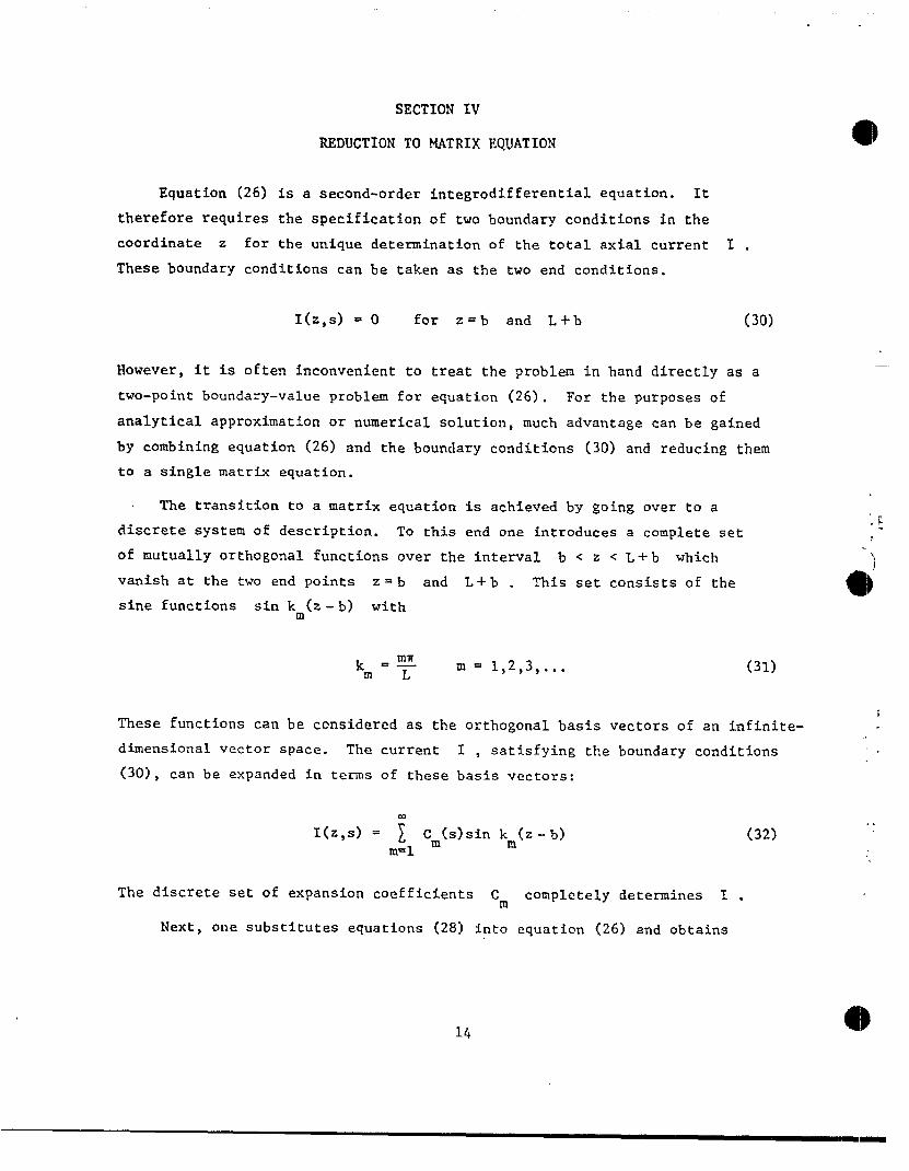
Equation (26) is a second-order integrodifferential equation. It

therefore requires the specification of two boundary conditions in the

coordinate z for the unique determination of the total axial current 1 .

These boundary conditions can be taken as the two end conditions.

1(2,s) = o for z=b and L+b (30)

However, it is often inconvenient to treat the problem in hand directly as a

two-point boundary-value problem for equation (26). For the purposes of

analytical approximation or numerical solution, much advantage can be gained

by combining equation (26) and the boundary conditions (30) and reducing them

to a single matrix equation.

The transition to a matrix equation is achieved by going over to a

discrete system of description. To this end one introduces a complete set

of mutually orthogonal functions over the interval b < z < L+b which

vanish at the two end points z=b and L+b . This set consists of the

sine functions sin km(z-b) with

mxkL .— m= 1,2,3, ...m

(31)

These functions can be considered as the orthogonal basis vectors of an infinite-

dimensional vector space. The current I , satisfying the boundary conditions

(30), can be expanded in terms of these basis vectors:

I(z,s) = ~ C (s)sin k (z-b)In m

In=1(32)

. .

The discrete set of expansion coefficients Cm completely determines I .

Next, one substitutes equations (28) into equation (26) and obtains

14

where

and

~ ~ W (s)A (s)sin pnZ - Y* ~ Wn(S)Bn(S)COS Pnzn n

n=l n=O

–inc(z,s)=-sEE02

L+b

[

aAn(s) = dz’sin pnz’ ~I(z’,s)

IL+b

Bn(s) = dz’cos pnZ’I(Z’,S)

(33)

(34)

(35)

b

Performing an integration by parts in equation (34) and making use of equation

(30), one finds t’nat An and Bn are related:

An(s) = - pnBn(s) (36)

S,,bstitutingequation (32) into equation (35), one has

aBn(s) = ~ amCm(s) (37)

~.1

where

JL+b

a= dz’cos pnz’ sin km(z’ -b) (38)

b

Note that the index n runs from O to ~ while the index m runs from

lto’=.

Equation (33) can be regarded as a vector relation in the infinite-

dinensional vector space. The component of this relation along the basis

vector sin km(z-b) can be obtained by multiplying equation (33) by

sin km(z- b) and integrating over z from b to L+b . The derivative

in the first term is again treated by integration by parts. The result then is

i ~nm~~~n(s~An(s) + Y2 i anmwn(s)B (s) = Din(s)n=l

nn=O

(39)

—

15

where

and

. .

. .L+b

t3m =\

dz sin pnz cos km(z-b)

b

L+bDin(s)= S~o

Idz sin km(z-b)~$c(z,s)

b

It is not difficult to see that am and @nm are related:

Substituting

a matrix equation

where

The matrix M is

(40)

(41)

3nmkm = - pnam (42)

equations (36), (37) and (42) into equation (39), one obtains

for the expansion coefficientsCL :

~ Mm2(S)C2(S) = Din(s)%=1

symmetric (MmL = M~m) but not Hermitian (MmE 4 M~m) .

16

(43)

—

—

-

SECTION V

APPROXIMATE ANALYTICAL SOLUTION

The matrix equation (43) is a concise and exact formulation of the

simulator/test-object interaction problem. From the standpoint of solving

the problem it is also a convenient starting point. For example, an accurate

numerical solution can always be obtained by using standard methods in numerical

matrix calculus. In the following, however, an approximate analytical solution

will be constructed instead.

The approximation employed below is based on the observation that the

diagonal elements of the matrix M in equation (43) are considerably greater

than the off-diagonal elements. The reason behind this disparity is as follows.

If one examines closely the structure of the matrix element Mmk given in

equation (44), one finds that the combination a~ank has the most violent

variation with the summation index n . It has therefore a great effect on

the value of MmL . The factor am can be evaluated from equation (38):

km

a=nm [

COS pnb - (-l)mcos pn(L+b)k: - p2 1

n

(45)

It assumes both positive and negative values. In an off-diagonal matrix element

M with m#f.r.k

, these positive and negative values of a and a to anl.

considerable extent mutually cancel out during the summation over n , However,

the situation is different with a diagonal matrix element ?4m . Vithm=f,

the product anmant becomes the square a: which is always positive. It

contributes constructively to Mm , and adds up to a large value. For small

values of m and t , sample numerical calculations show that the diagonal

elements are one order of magnitude greater than the off-diagonal ones. The

disparity is expected to increase for larger values of m and g .

This property of the matrix elements is the basis of an approximation

scheme for solving the matrix equation (43). One first rearranges the equation

in the form

Mm(s)cm(s) = Din(S) - ~ Mm2(s)ct(s)1=1t#m

(46)

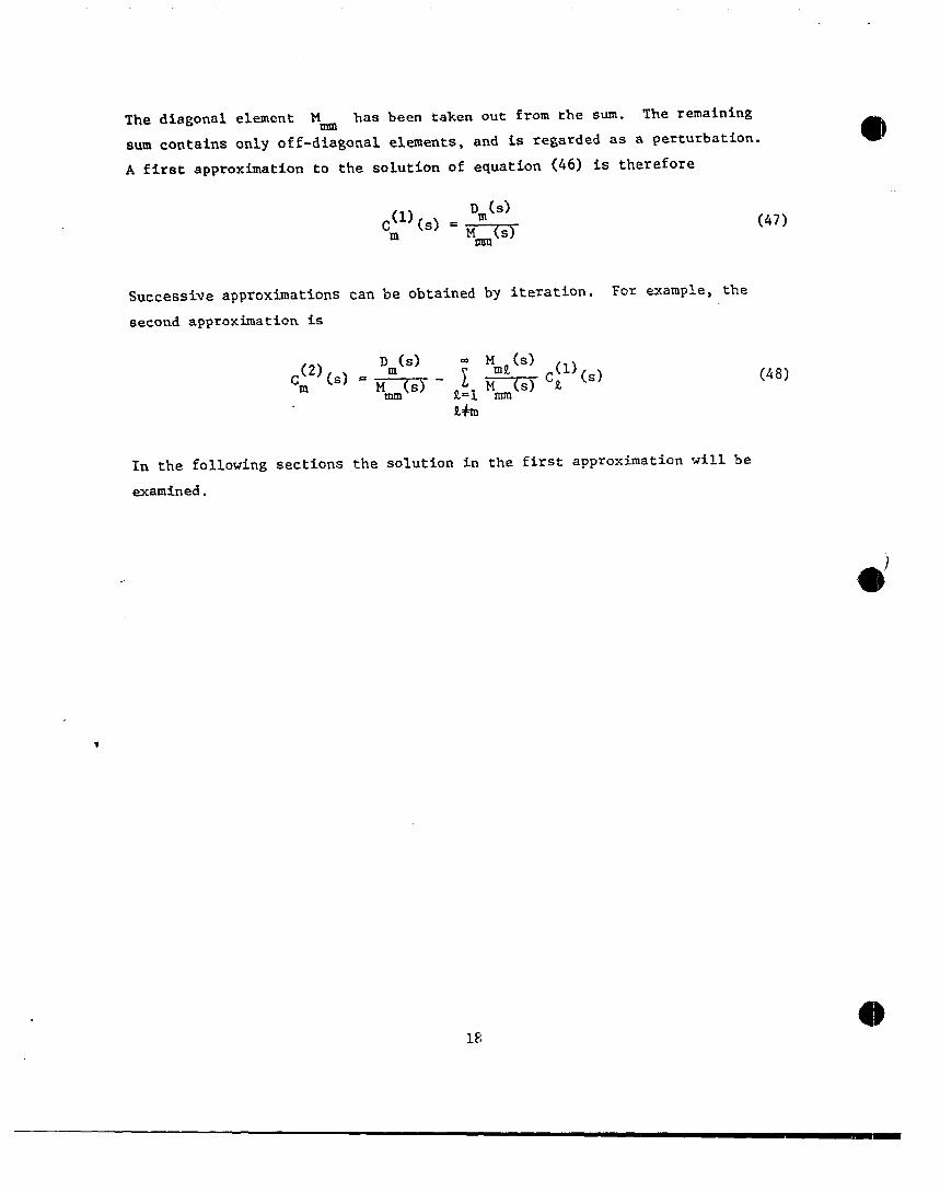
The diagonal element Mm has been taken out from the sm. The remaining

sum contains only off-diagonal elements, and is regarded as a perturbation.

A first approximation to the solution of equation (46) Is therefore

Successive approximations

second approximation i-s

#e\

Jo(, ) ..*m mm

can be obtained by iteration, For example, the

9A

In the following sections the solution in the first approxfiation will be

examined.

s

(47)

(48)

——

—

SECTION VI

COMPLEX-FREQUENCY-PLANE SINGLMRITIES

In the first approximation of equation (47) the total axial current

induced on the cylinder is given by

o D (S)I(z,s) = ~ -sin kn(z-b)

m=l mm

In the time domain this current becomes

~

C+jco m Din(s)I(z,t) =~

2mjds est Im=~ Mm(s)

sin km(z-b)

c-jm

where C is an appropriate positive constant. The value of the integral

(49)

(50)

is dependent on the singularities of the integrand in the left half of the

complex s-plane. The parameters of these singularities can be used to

characterize the excitation of the cylinder.

The s-plane singularities can be grouped into three classes. The first

class consists of singularities of the factor D By equation (41) theseIn”

singularities are introduced by the frequency dependence of the incident.

electric field E~c . The second class consists ”of”sfngularitfes of the

factor ?4 By equation (44) these singularities are contained in the func-mm”

tion W defined in equation (29). From the well-known analytical propertiesn

of the modified Bessel functions, one concludes that these s~ngularities are

branch cuts with branch

Y

oints determined by the vanishing of the argument of

the function Ko( y2+p~a) . By equation (7) the branch points are located at

s WY n = 0,1,2, ... (51)

along the imaginary axis. They are characteristic of the parallel-plate

waveguidc, and depend neither on the length L nor the radius a of the

cylinder. In fact they correspond to the excitation thresholds of the wave-

guide propagation modes. Examples of these waveguide node singularities are

shown in figure 2.

19

“.

e3

2

1

,.. –,

I -1

-2

1’

Figure 2. Branch-Cut Singularities in the Complex-Frequency Plane

Characterizing the Waveguide Modes

20

The third class of s-plane singularities consists of the zeros of Mmm .

They give rise to poles in the integrand of equation (50), and are determined

by solving the transcendental equation

()2

Mm(s) = ~ ~+ p: Wn(s)u:m =n=O c

The solutions depend on all the parameters h,

o m = 1,2,3,. .. (52)

L and a of the model. They

can be interpreted as the natural frequencies of certain natural modes of the

surface current on the cylinder. For each m , there are two solutions of

equation (52) which form a complex-conjugate pair. They lie in the second.

and third quadrants of the s-plane. The natural modes corresponding-to these

natural frequencies are the sine functions in equation (50). Thus, in this

approximation, the natural modes are simple sinusoidal currents.

Let the solution of equation (52) in the second quadrant be denotedby

s The other solution is its complex conjugate s: in the third quadrant.m“Decompose sm into its real and imaginary parts:

Sm = s; + j s“m

(53)

In principle, s: and s; can be obtained accurately by numerical techniques.

In the following, however, one will be content with deriving approximate ..analytical expressions. The method of approximation will be based on the

assumption that the two poles lie close to the imaginary axis, so that they

can be approximately located by observing their influence on the behavior of

M along the imaginary axis.

On the imaginary s-axis, let

S=jf.o, *y=jk (54)

where u and k are both real and vary from -= to co . They are related by

to=kc (55)

-21

.

The function Wn can be decomposed into

Wn(jL$)= w:(u))

By equations (1S) and {29), one has

its real and imaginary parts:

+ jw’’(ul) (56)

-~ Jo(~a)y(~a)0(k2 -p2)on

n n

(57)

where 3 and Y are the Bessel and Neumann functions”,ar.d 0 is the unito 0

step function:

I1 X>o

8(X) =

o X<o

(58)

The square roots in equation (57) are all considered positive.

In a similar manner the value of M along the imag%nary axis can be

decomposed into its real and tiaginary parts:

with

M“(w) = nN$+4’’~(”)~m

(59)

(60)

When jf.ois close to the solution s of equation (52) in the second quadrant,m

can be seen to pass through a zero. This property is used to determine

approximately:

a

22

M&(s:) = O (61)

u

which is a transcendental equation involving real quantities only. It iS

simpler to solve than the original complex equation (52).

A practical technique to solve equation (61) iS bY iteration. Using

equation (60) one can rewrite it as

m

[ 1I P2W’(S’’)C?%II=c

n=o n n m nmsm

: w% ’’)c12nmnm

n=O

(62)

The iteration is performed by successively substituting trial solutions into

the right-hand side and deriving improved approximations on the left-hand side.

In the appendix it is shown th?.t,in the infinitely thin cylinder limit, the

solution of equation (62) is simply

(63)

?ence, for a thin cylinder , one can use thts result to start the iteration.

An improved approximation to s“ is thereforem

s“ = cm

[

~ p% ’(k C)a2n=onnmnm

~ W’(k C)a2nmnm

il=o

(64)

The following calculation will be based on this approximate solution of

equation (61).

In the neighborhood of this solution, X& has the following approxi-

mate expansion:

(65)

23

. .

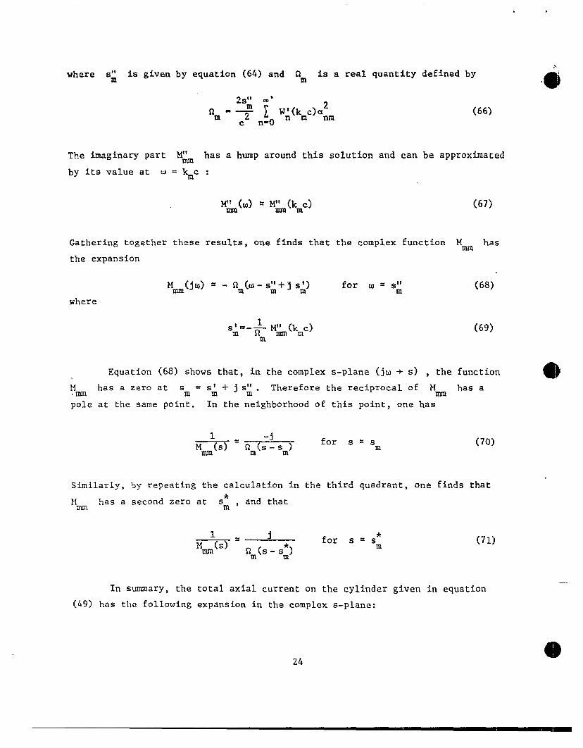
.,where s; is given by equation (64) and Qm 5s a real quantity defined by

.&!, =*

flm= + I W;fkmc)”:m (66)c n=O

Tke imaginary part M“ has a hump around this solution and can be approximated

by its value at m = kmc :

M“(lo) = M&(kmc) (67)

Gathering together these results, one finds that the complex function M has

the expansion

Mm(ju) = - nm(u-s;+js;) for u = s“ (68)m

where

1 M“ (kmc)s;=-_nm mm (69)

Equation (68) shows that, in the complex s-plane (jm + s) , the function *

m has a zero at Sm= s~+js”.~.f Therefore the reciprocal of Mm has am

pole at the same point. In the neighborhood of this point, one has

1 -jMm(s) = rtm(s-sm)

for s = sm (70)

Similarly, by repeating the calculation in the third quadrant, one finds that

I.lm has a second zero

In summary, the

(49) has the following

*at s

Kn, and that

,+. z ~ for s = s*‘mm nm(s -s:)

m (71)

total axial current on the cylinder gtven ~n equatton

expansion in the complex s-plane:

24

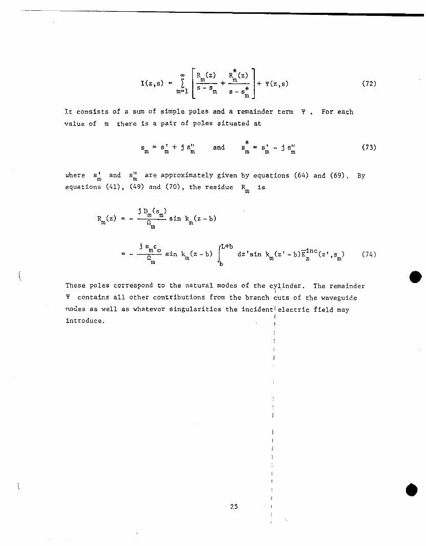
I(z,s) = im=1

RJz) R;(z)—+—

1

+ Y(z, s)s-s

m s-s*m

It consists of a sum of simple poles and a remainder term Y . For each

value of m there is a pair of poles situated at

*s = s! -+j s!! andm m

sn-l

;-js:=sm

(72)

(73)

where s’ and s“ are approximately given by equations (64) and (69). By

equation: (41), (;9) and (70), the residue Rm is

j Dm(sm)Rm(z) = - —

‘Omsin km(z-b)

j Smco

IL+b

=-Qm

sin km(z-b) –~=(z’,sm)dz’sin km(z’-b)E (74)

b

These poles correspond to the natural modes of the cylinder. The remainder

Y contains all other contributions from the branch cuts of the waveguide

nociesas well as whatever singularities the incident~electric field mayJ

introduce. Y

—

i

SECTION VII

NUMERICAL RESULTS

The three quantities s; , s: and f? , characteristic of the simple-pole

singularities in the complex s-plane, are given analytically in equations (64),

(66) and (69). In the following they are evaluated numerically as functions

of the geometrical parameters h , a , L and the natural-mode index m . One

takes a case in which the cylinder is situated midway between the two parallel

plates, so that

b = (h- L)/2 and L+b = (h+L)/2 (75)

This is a highly symmetric situation. Accordingly, the quantity anm assumes

a simple form:

r nl! pnLCos — Cos —

2 2m odd, n even

pnLa .nm

k~~~ “n Y ‘in ~ n ‘Ven’ n 0“n

[o otherwise

(76)

Thus am is nonzero only if n and m are of opposite parities.

The numerical calculation is performed for the first six natural modes

(m=l to6) . One picks four values of the ratio a/L :

a–= 0.003, 0.01, 0.03, 0.1L

{77)

and three values of the ratio L/h :

L–= 0.2, 0.5003$ 0.8003h

(78)

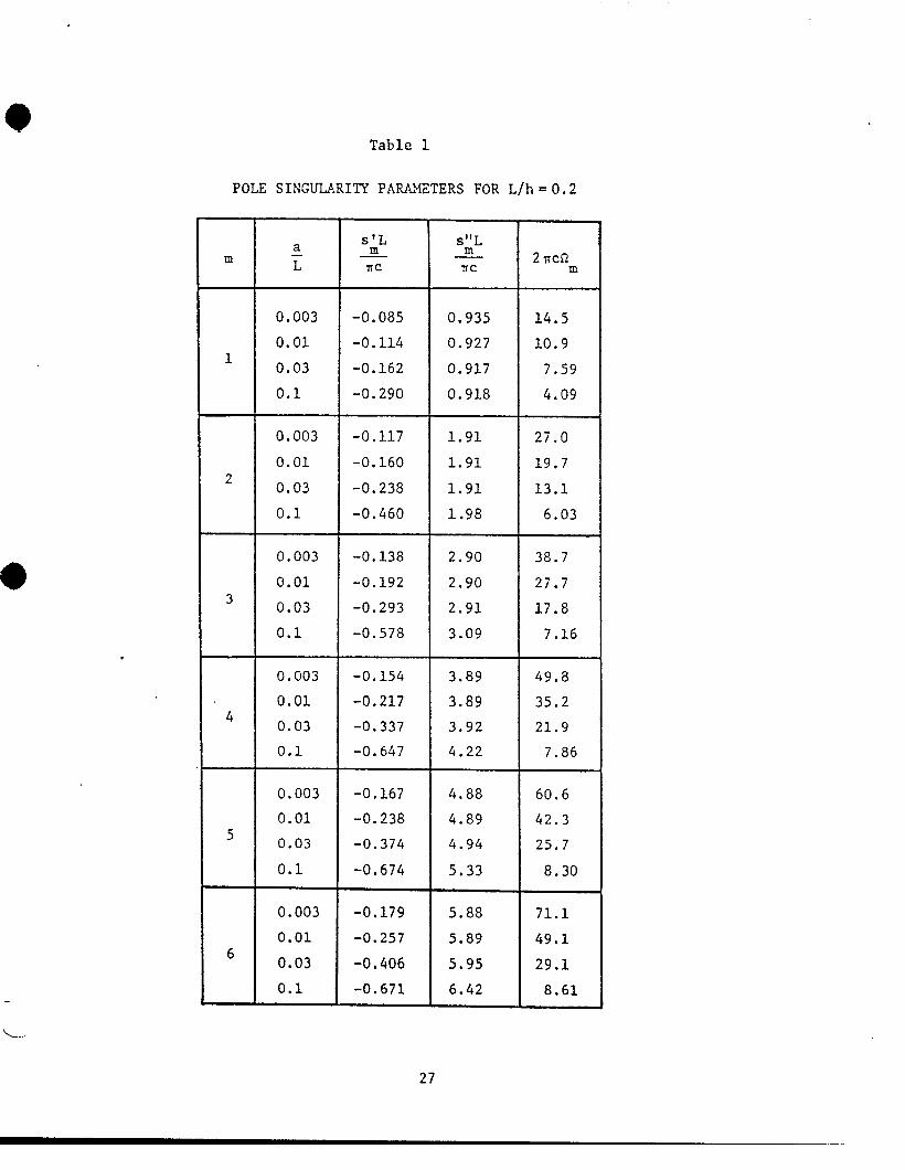
The results are shown in tables 1 to 3. They are also plotted in figures 3 to 5.

The odd choices of the last two values of L/h in equation (78) need

Inrnediateexplanation. When the ratio L/h is given simple, rational values

26

.

Table 1

POLE SINGULARITY PARAMETERS FOR L/h=O.2

D

1

2

3

4

5

6

0.003

0.01

0.03

0.1

0.003

0.01

0.03

0.1

0.003

0.01

0.03

0.1

0.003

0.01

0.03

0.1

0.003

0.01

0.03

0.1

0.003

0.01

0.03

0.1

~lL

mlrc

-0.085

-0.114

-0.162

-0.290

-0.117

-0.160

-0.238

-0.460

-0.138

-0.192

-0.293

-0.578

-0.154

-0.217

-0.337

-0.647

-0.167

-0.238

-0.374

-0.674

-0.179

-0.257

-0,406

-0.671

s“Lml’rc

0.935

0.927

0.917

0.918

1.91

1.91

1.91

1.98

2.90

2.90

2.91

3.09

3.89

3.89

3.92

4.22

4.88

4.89

4.94

5.33

5.88

5.89

5.95

6.42

2?lCnm

14,5

10.9

7.59

4.09

27.0

19.7

13.1

6.03

38.7

27.7

17.8

7.16

49.8

35.2

21.9

7.86

60.6

42.3

25.7

8.30

71.1

49*1

29.1

8.61

27

. .

Table 2

POLE SINGULARITY PARAMETERS FOR L/h =0.5003

s;L s“Lm

m: —

2rcflXc llc m

0.003 -0.052 0.952 19*1

0.01 -0.064 0.950 15.51

0.03 -0.081 0.950 12.2

0.1 -0.109 0.963 8.73

0.003 -0.126 1.94 26.7

0.01 -0.174 1.93 19.22

0.03 -0.266 1.91 12.5

0.1 -0.557 1.99 5.35

0.003 -0.094 2.90 49.3

0.01 -0.119 2.91 38.6

3 0.03 -0.155 2.93 28.9

0.1 -0.186 3.03 18.4

0.003 -0.165 3.93 49.1

0.01 -0.236 3.92 34.14 0.03 -0.379 3.93 20.6

0.1 -0.848 4.27 6.47

0.003 -0.117 4.88 76.4

0.01 -0.152 4.90 58.65

O*O3 -0.199 4.95 42.3

0.1 -0.176 5.10 25.1

0.003 -0.191 5.92 69.8

0.01 -0.280 5.92 47,4

60.03 -0.458 5.97 27,1

0.1 -0.976 6.61 6.541

28

Table 3

POLE SINGULARITY PARAMETERS FOR L/h= O.8003

+

an

Y

0.003

0.011

0.03

0.1

0.003

0.012

0.03

0.1

s’Lmlrc

-0.114

-0.154

-0.226

-0.431

-0.128

-0.177

-0.266

-0.504

3

4

0.003.

0.01

0.03

0.1

0.003

0.01

0.03

0.1

-0.110

-0.151

-0.220

-0.327

-0.061

-0.075

-0.090

-0.0651

I I

I0.003 I -0.129

I0.01

50.03

0.1

I0.003

0.016 ’003

.

0.1

-0.180

-0.270

-0.447

-0.182

-0.265

-0.435

-1.25

s“Lmllc

0.956

0.947

0.936

0.952

1.97

1.97

1.99

2.15

2.97

2.98

3.01

3.21

3.95

3.96

3.98

4.04

4.88

4.87

4.88

5.02

5.86

5.85

5.86

6.22

!Tfcflm

14.1

10.4

7.04

3.53

26.9

19.5

12.8

5.77

41.1

30.0

20.0

9.50

77.9

63.1

49,6

35.3

64.6

46.1

29.2

10.6

70.2

48.0

27.7

5,76

a/L=O

SJJ7TC

6

5

4

3

2

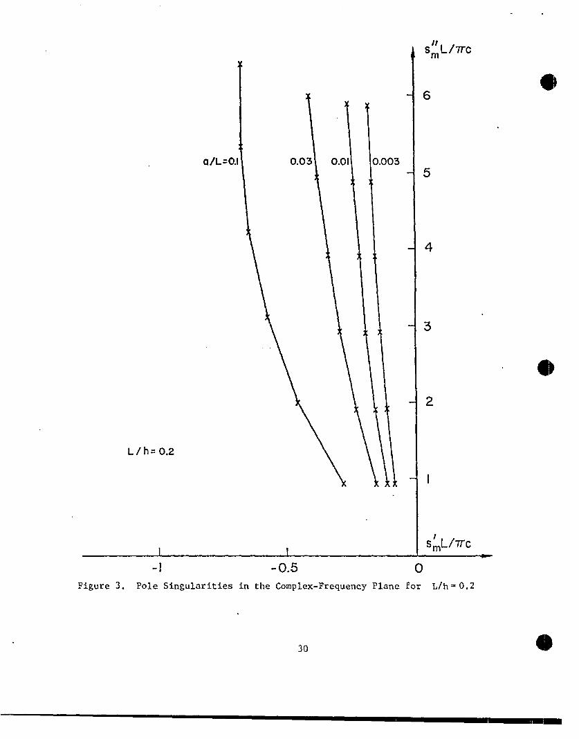
-1 -0.5 c1Figure 3. Pole Singularities in the Complex-Frequency Plane for L/h=O.2

30

I I-1 -0.5

s~LnTc

5

4

3

2

I

Figure 4. Pole Singularities in the Complex-Frequency Plane for L/h=0.5003

r-..

31

!Jh =0.8003

).OC

,

I I-1 -0.5

s; L\?Tc

5

3

I

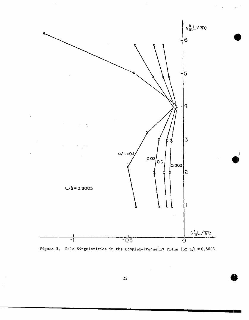
Ftgure 5. Pole Singularttfes in the Compl~-FrequeAcy Plane for L/h=O.8003

32

such as 0.5, it may happen that, for a certain pair of integers m and n ,

the following equality holds:

km=pn

(79)

In this event one finds a logarithmic divergence in equation (64) arising from

the exact vanishing of the argument of the function K. or Y. . This

divergence nevertheless is not really there, and can be traced back to a

harmless term vanishing as c En c in the function Mm . It is introduced

into the picture through the iterative scheme of equation (62) and the use of

knc as the first trial solution in equation (64). It can be easily avoided

by starting the iteration with a slightly different trial solution. An alter-

native procedure is to alter the ratio L/h by a small amount. For example,

the ratio L/h = 0.5 can be replaced by L/h = 0.5003 , thereby destroying

the equality (79).

Form =lto6andn of opposite parity to m , the equality is not

satisfied for L/h = 0.2. “However, for L/h = 0.5 , equation (79) holds :OF

m=l,3and5. For L/h = 0.8 , it holds for m = 4 . Accordingly, in the

numerical calculation, the last two simple values of L/h are changed slightly

to 0.5003 and 0.8003.

Even though no divergence really occurs, equation (79) still clearly

represents a condition of resonance and should lead to observable effects.

The resonance results from the equality of the wavelengths of certain charac-

teristic excitations on the cylinder and in the waveguide. Its effects are

quite evident in figures 3 to 5. At precisely those values of m enumerated

in the preceding paragraph, the complex poles show a decided shift toward

the imaginary axis. This means that the corresponding natural modes of the

cylinder are only weakly damped. Thus, under the excitation of a broadband

incident wave, the response of the cylinder will be predominantly in these

special modes.

All the results in tables 1 to 3 are of course obtained by using the

first-iterated solution of equation (62). The quality of this solution can

..

33

be measured by comparing the output value of s: with its input trial value

lcmc. The tables show that these two values are very close. Specifically,

the calculated value of s~L/?rc is very close to m . This agreement can be

taken as an indication of the reliability of the first-iterated solution.

34

SECTION VIII

CONCLUSIONS

P:-

—

It is possible

fiumericalresults.

The effects of

in figures 3 to 5.

to draw a number of general conclusions from the specific

the simulator/test-object interaction are clearly seen

The locations of the poles in the complex-frequency plane,

corresponding to the natural modes of the current on the cylinder, are strongly

dependent on the length-to-separation ratio L/h . When L/h is small, the

dimensions of the simulator are much greater than those of the test object.

The simulator/test-object interaction is weak, at least for the lowest few

natural modes. For example, the distribution of the poles in figure 3 for

L/h = 0.2 is not substantially different from that in the case of a thin

cylinder in free space (ref. 3). As the ratio L/h is increased, the effects

of the interaction strengthen: the poles are shifted violently around. The

dependence of their movement on L/h , however, is not monotonic but rather

oscillatory and in the nature of resonances. For a given ratio L/h, modes

that satisfy the resonance condition (79) are heavily favored by the simulator/

test-object interaction, in the sense that they are only weakly damped. These

resonant cases are exemplified by the numerical results in figures 4 and 5.

The poles, however, are not sufficient in themselves to provide a complete

measure of the simulator/test-object interaction. The presence of the simulator

structure introduces additional singularities into the complex-frequency plane.

For the parallel-plate bounded-wave simulator in this problem, these singularities

consist of an infinite number of branch cuts. The contribution from the branch

cuts must be considered if one is to obtain a full characterization of the simu-

later/test-object interaction.

The numerical results of this study are based on an approximate, analytical

formula for the solution of an exact matrix equation. It will be worthwhile

to attempt an accurate , numerical solution of the matrix equation directly.

Such a solution is feasible with the availability of large, advanced computers.

It will not only provide accurate technical data, but will also represent a

valuable standard whereby the reliability of future analytical investigations

can be gauged.

35

REFERENCES

[1] Baum, C.E., “Impedances and Field Distributions for Parallel-Plate

Transmission-Line Simulators,” Sensor and Simulation Notes, Yote 21,

Air Force Weapons Laboratory, Kirtland Air Force Base, NM, 1966.

[2] Magnus, !?.and F. Oberhettinger, Formulas and Theorems for the Functions

of Mathematical Physics, Chelsea, New York (1949), P.21.

[3] Marin, L., “Natural Modes of Certain Thin-Wire Structures,” Interaction.

Notes, Note 186, Air Force Weapons Laboratory, Kirtland Air Force Base,

NM, 1974.

..

-d 1.

36

APPENDIX

THIN-CYLINDER LIMIT

In the thin-cylinder limit (a/L + O) equation (62) can be shown to have

the simple solution s: = t kmc .

By equation (45) the quantity a;-4

varies like n for large n . Thus

the contribution to the two sums in equation (62) comes mainly from terms of

small n . Because of this property, one can replace the function W’ by itsn

thin-cylinder limit at small n . By equation (57) one has

Therefore equation (62) becomes

2

()

s11m—c

f 22+ pnanm= n=O n

f ~a:mn=O ‘n

BY equation (42) it can also be rewritten as

2

0

s“m—c = k2m

(Al)

(A2)

(A3)

The two sums can be evaluated by invoking equations (38) and (40):

L

1=—Lb4

37

r

j. $ U2. ‘+b~z L+b

--1%

[[

m 1

dz’sin k (z- b)sin km(z’-b) ~nm m

+- Cos pnz Cos pnz’ en n=O n

1=_Lh4

(A4)

where use has been made of the identities

i $sin Pn’’in Pn’’=$ ’(’””)n=O n

$ ~cos Pn’cos Pn’’=; ~(’-”)~.o En

for b < Z,Z’ < L+b . Substituting equations (A4) into equation (A3) one

obtains the simple result

s ‘[ = f kmcm

38

.

(A6)

--

a“