GeophysicalResearchLetters

RESEARCHLETTER10.1002/2014GL062748

Key Points:• The IMF By has an impact on thehigh-latitude thermospheric density

• Positive/negative By e!ect in NHresembles negative/positive By e!ectin SH

• Thus, the IMF By is an importantsource for the north-southasymmetry

Correspondence to:Y. Yamazaki,y.yamazaki@lancaster.ac.uk

Citation:Yamazaki, Y., M. J. Kosch, and E. K.Sutton (2015), North-south asymme-try of the high-latitude thermosphericdensity: IMF BY e!ect, Geophys. Res.Lett., 42, doi:10.1002/2014GL062748.

Received 3 DEC 2014Accepted 17 DEC 2014Accepted article online 22 DEC 2014

This is an open access article underthe terms of the Creative CommonsAttribution License, which permits use,distribution and reproduction in anymedium, provided the original work isproperly cited.

North-south asymmetry of the high-latitude thermosphericdensity: IMF BY e!ectYosuke Yamazaki1, Michael J. Kosch1,2, and Eric K. Sutton3

1Department of Physics, Lancaster University, Lancaster, UK, 2South African National Space Agency, Hermanus,South Africa, 3AFRL, Kirtland Air Force Base, NewMexico, USA

Abstract Previous studies have established that the y component of the interplanetary magneticfield (IMF By) plays a role in the north-south asymmetry of the high-latitude plasma convection and wind.The e!ect of the positive/negative IMF By in the Northern Hemisphere resembles the e!ect that thenegative/positive IMF By would have in the Southern Hemisphere. In this study, we demonstrate thatthe IMF By e!ect can also contribute to the hemispheric asymmetry of the thermospheric density. Weuse high-accuracy air drag measurements from the CHAllenging Minisatellite Payload (CHAMP) satelliteand SuperMAG AE index during the period 2001–2006 to examine the response of the high-latitudethermospheric density to geomagnetic activity. Our statistical analysis reveals that the density response at400 km is greater in the Southern Hemisphere under positive IMF By conditions, and greater in the NorthernHemisphere under negative IMF By conditions. The results suggest that the IMF By e!ect needs to be takeninto account in upper atmospheric modeling for an accurate description of high-latitude densities duringperiods of enhanced geomagnetic activity.

1. Introduction

The interaction between the solar wind and magnetosphere generates electric fields in the high-latitudeionosphere. These electric fields cause the ionospheric plasma to convect around the regions of positiveand negative electric potentials. It is well known that the patterns of these convection “cells” are dependenton the strength and orientation of the IMF [e.g., Cousins and Shepherd, 2010]. Particularly, the role of the IMFBy has been found to produce an asymmetry between the Northern Hemisphere and Southern Hemisphereconvection patterns. For a nonzero IMF By condition, the cell patterns in the Northern Hemisphere resemblethose in the Southern Hemisphere for the opposite sense of the IMF By .

The neutral gas in the high-latitude regions tends to be accelerated, or “dragged”, in the direction of therapid motion of the ions due to collisional interactions between plasmas and neutrals. This ion drag e!ectbrings about similarities in the patterns of high-latitude thermospheric wind and ion convection [e.g.,Richmond and Lu, 2000]. Förster et al. [2008] showed that the IMF By e!ect can cause a north-southasymmetry in the high-latitude thermospheric wind in a similar manner as in the ion convection.

The IMF By e!ect on the wind may have a broad impact on the neutral atmosphere. For example, changesin the horizontal wind system can cause the vertical motion of the air, which leads to adiabatic heatingor cooling of the gas. Therefore, it is possible that the temperature, composition, and mass of the upperatmosphere are altered as a result of the IMF By e!ect on the wind, although it is di"cult to predict what andhowmuch the actual variations might be.

Crowley et al. [2006] used a coupled thermosphere-ionosphere general circulation model to study the IMFBy e!ect on the thermosphere. They ran simulations with di!erent ion convection patterns representativeof di!erent IMF By conditions. Their results suggested that the density distribution in the high-latitudethermosphere systematically changes when the ion convection pattern is changed. Although e!orts havealso been made to provide observational evidence for the IMF By e!ect on the thermospheric density[e.g., Immel et al., 1997, 2006; Kwak et al., 2009], an important piece of evidence has been missing, i.e.,the hemispheric asymmetry associated with the IMF By e!ect. In this paper, we will provide evidencethat the north-south asymmetry of the high-latitude thermospheric density can arise from the IMFBy e!ect.

YAMAZAKI ET AL. ©2014. The Authors. 1

Geophysical Research Letters 10.1002/2014GL062748

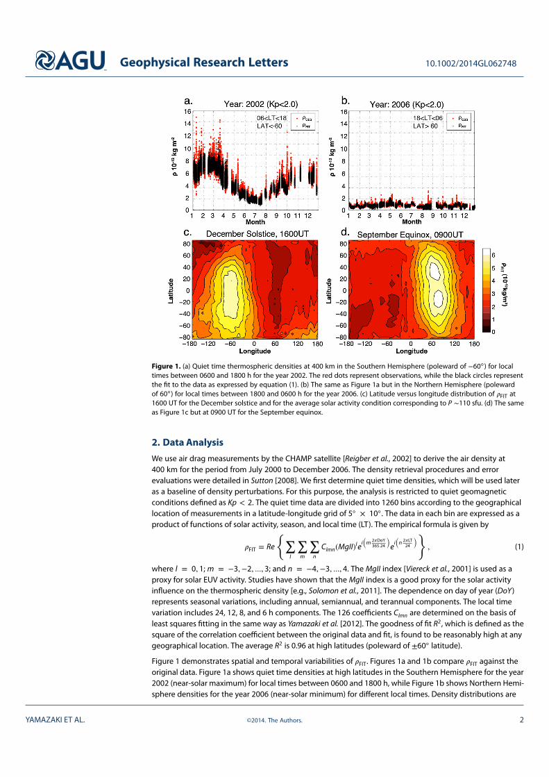
Figure 1. (a) Quiet time thermospheric densities at 400 km in the Southern Hemisphere (poleward of !60!) for localtimes between 0600 and 1800 h for the year 2002. The red dots represent observations, while the black circles representthe fit to the data as expressed by equation (1). (b) The same as Figure 1a but in the Northern Hemisphere (polewardof 60!) for local times between 1800 and 0600 h for the year 2006. (c) Latitude versus longitude distribution of !FIT at1600 UT for the December solstice and for the average solar activity condition corresponding to P "110 sfu. (d) The sameas Figure 1c but at 0900 UT for the September equinox.

2. Data Analysis

We use air drag measurements by the CHAMP satellite [Reigber et al., 2002] to derive the air density at400 km for the period from July 2000 to December 2006. The density retrieval procedures and errorevaluations were detailed in Sutton [2008]. We first determine quiet time densities, which will be used lateras a baseline of density perturbations. For this purpose, the analysis is restricted to quiet geomagneticconditions defined as Kp < 2. The quiet time data are divided into 1260 bins according to the geographicallocation of measurements in a latitude-longitude grid of 5! # 10!. The data in each bin are expressed as aproduct of functions of solar activity, season, and local time (LT). The empirical formula is given by

!FIT = Re

!"l

"m

"n

Clmn(MgII)lei#m 2"DoY

365.24

$ei#n 2"LT

24

$%, (1)

where l = 0, 1;m = !3,!2, ..., 3; and n = !4,!3, ..., 4. The MgII index [Viereck et al., 2001] is used as aproxy for solar EUV activity. Studies have shown that the MgII index is a good proxy for the solar activityinfluence on the thermospheric density [e.g., Solomon et al., 2011]. The dependence on day of year (DoY)represents seasonal variations, including annual, semiannual, and terannual components. The local timevariation includes 24, 12, 8, and 6 h components. The 126 coe"cients Clmn are determined on the basis ofleast squares fitting in the same way as Yamazaki et al. [2012]. The goodness of fit R2, which is defined as thesquare of the correlation coe"cient between the original data and fit, is found to be reasonably high at anygeographical location. The average R2 is 0.96 at high latitudes (poleward of ±60! latitude).

Figure 1 demonstrates spatial and temporal variabilities of !FIT. Figures 1a and 1b compare !FIT against theoriginal data. Figure 1a shows quiet time densities at high latitudes in the Southern Hemisphere for the year2002 (near-solar maximum) for local times between 0600 and 1800 h, while Figure 1b shows Northern Hemi-sphere densities for the year 2006 (near-solar minimum) for di!erent local times. Density distributions are

YAMAZAKI ET AL. ©2014. The Authors. 2

Geophysical Research Letters 10.1002/2014GL062748

presented in Figures 1c and 1d for di!erent seasons and universal times, for an average solar activity condi-tion corresponding to P "110 sfu. Here P represents the solar activity index by Richards et al. [1994], and sfustands for solar flux unit. Examples presented in Figure 1 illustrate basic features of quiet time thermosphericdensity known from previous studies [see, e.g., Qian and Solomon, 2012, for a review].

We define density perturbations $! as the di!erence between the measurements and quiet time valuesas expressed by (1). The density perturbations are analyzed in the Magnetic Apex coordinate system[Richmond, 1995] as a function of magnetic latitude (MLAT) and magnetic local time (MLT) with a grid size of5! # 1 h.

We use hourly values of the SuperMAG AE index [Newell and Gjerloev, 2011] to characterize high-latitudegeomagnetic activity. Studies have shown that the typical response time of thermospheric densities togeomagnetic activity is less than 2 h at high latitudes and about 4 h at low latitudes [Sutton et al., 2009;Ritter et al., 2010]. Since our study focuses on the high-latitude densities, we use AE values averaged for thepresent hour and 1 h prior. Our average quiet time densities correspond to an AE index of approximately150 nT, and thus, the density perturbations are examined as a function of AEd =AE!150 for positivevalues of this parameter. The density perturbations are binned in 50 nT window of AEd up to 400 nT, and intoone bin for larger values. A linear regression analysis is then performed using the median value of $! andAEd in each bin. This median filter e!ectively eliminates outliers.

3. Results andDiscussion

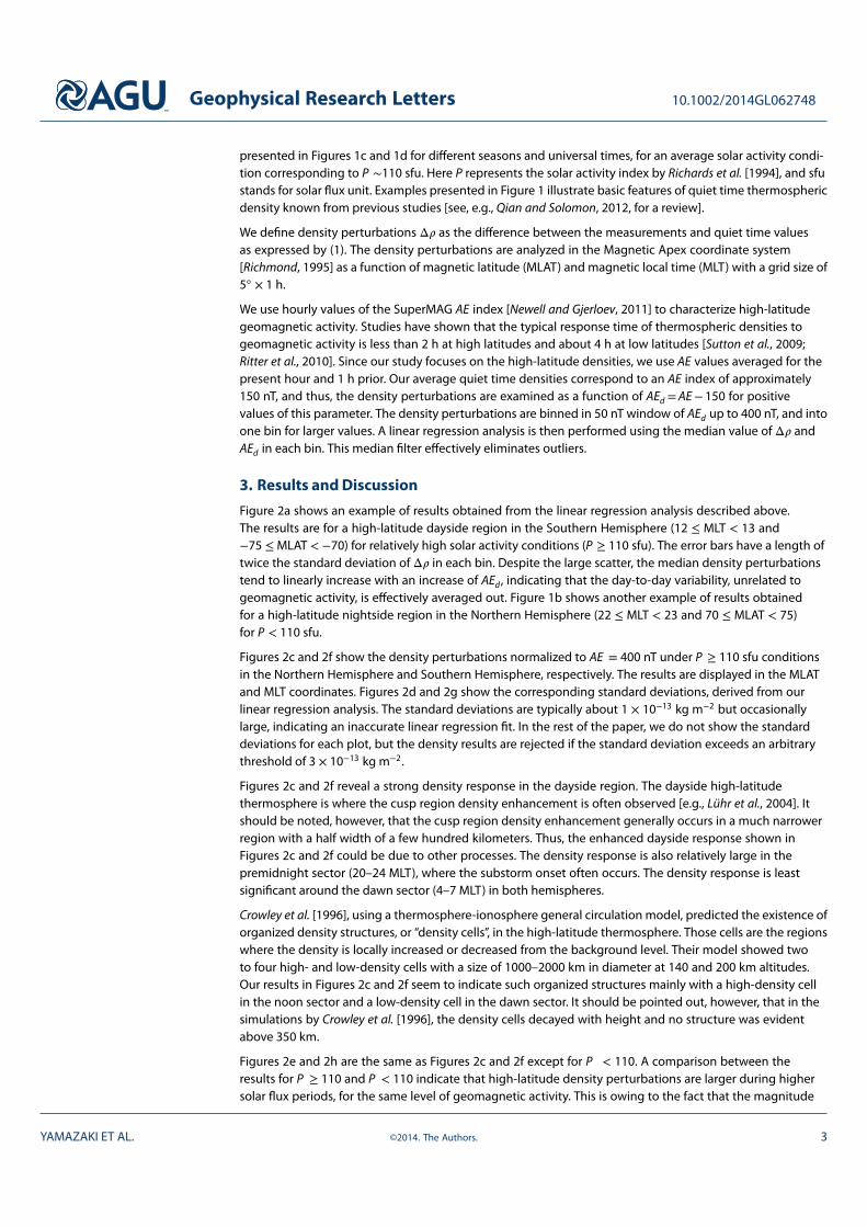
Figure 2a shows an example of results obtained from the linear regression analysis described above.The results are for a high-latitude dayside region in the Southern Hemisphere (12 ! MLT < 13 and!75 !MLAT < !70) for relatively high solar activity conditions (P " 110 sfu). The error bars have a length oftwice the standard deviation of $! in each bin. Despite the large scatter, the median density perturbationstend to linearly increase with an increase of AEd , indicating that the day-to-day variability, unrelated togeomagnetic activity, is e!ectively averaged out. Figure 1b shows another example of results obtainedfor a high-latitude nightside region in the Northern Hemisphere (22 ! MLT < 23 and 70 ! MLAT < 75)for P < 110 sfu.

Figures 2c and 2f show the density perturbations normalized to AE = 400 nT under P " 110 sfu conditionsin the Northern Hemisphere and Southern Hemisphere, respectively. The results are displayed in the MLATand MLT coordinates. Figures 2d and 2g show the corresponding standard deviations, derived from ourlinear regression analysis. The standard deviations are typically about 1 # 10!13 kg m!2 but occasionallylarge, indicating an inaccurate linear regression fit. In the rest of the paper, we do not show the standarddeviations for each plot, but the density results are rejected if the standard deviation exceeds an arbitrarythreshold of 3 # 10!13 kg m!2.

Figures 2c and 2f reveal a strong density response in the dayside region. The dayside high-latitudethermosphere is where the cusp region density enhancement is often observed [e.g., Lühr et al., 2004]. Itshould be noted, however, that the cusp region density enhancement generally occurs in a much narrowerregion with a half width of a few hundred kilometers. Thus, the enhanced dayside response shown inFigures 2c and 2f could be due to other processes. The density response is also relatively large in thepremidnight sector (20–24 MLT), where the substorm onset often occurs. The density response is leastsignificant around the dawn sector (4–7 MLT) in both hemispheres.

Crowley et al. [1996], using a thermosphere-ionosphere general circulation model, predicted the existence oforganized density structures, or “density cells”, in the high-latitude thermosphere. Those cells are the regionswhere the density is locally increased or decreased from the background level. Their model showed twoto four high- and low-density cells with a size of 1000–2000 km in diameter at 140 and 200 km altitudes.Our results in Figures 2c and 2f seem to indicate such organized structures mainly with a high-density cellin the noon sector and a low-density cell in the dawn sector. It should be pointed out, however, that in thesimulations by Crowley et al. [1996], the density cells decayed with height and no structure was evidentabove 350 km.

Figures 2e and 2h are the same as Figures 2c and 2f except for P < 110. A comparison between theresults for P " 110 and P < 110 indicate that high-latitude density perturbations are larger during highersolar flux periods, for the same level of geomagnetic activity. This is owing to the fact that the magnitude

YAMAZAKI ET AL. ©2014. The Authors. 3

Geophysical Research Letters 10.1002/2014GL062748

Figure 2. (a, b) Examples of the relationship between AEd and density perturbations $! at 400 km. (c, f ) Distributions of the high-latitude density perturbations$! at 400 km for AE = 400 nT and P " 110 sfu. The average value of P and its standard deviation (in sfu) are also indicated, along with the average number of thedata points and its standard deviation. (d, g) Distributions of the standard deviation (SD) for the high-latitude density perturbations $! at 400 km for AE = 400 nTand P " 110 sfu. (e, h) The same as Figures 2c and 2f but for P < 110 sfu.

of density perturbations tends to increase with the background density. It is interesting to note that thedensity response in the dawn sector shows the opposite solar activity dependence. That is, the normalizeddensity perturbation is slightly lower for the higher solar activity condition.

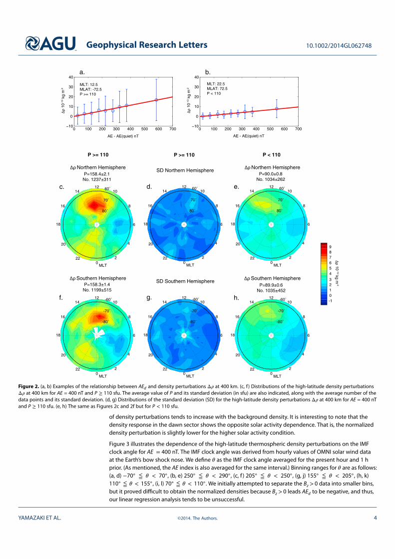
Figure 3 illustrates the dependence of the high-latitude thermospheric density perturbations on the IMFclock angle for AE = 400 nT. The IMF clock angle was derived from hourly values of OMNI solar wind dataat the Earth’s bow shock nose. We define # as the IMF clock angle averaged for the present hour and 1 hprior. (As mentioned, the AE index is also averaged for the same interval.) Binning ranges for # are as follows:(a, d) !70! # # < 70!, (b, e) 250! # # < 290!, (c, f ) 205! # # < 250!, (g, j) 155! # # < 205!, (h, k)110! # # < 155!, (i, l) 70! # # < 110!. We initially attempted to separate the Bz >0 data into smaller bins,but it proved di"cult to obtain the normalized densities because Bz >0 leads AEd to be negative, and thus,our linear regression analysis tends to be unsuccessful.

YAMAZAKI ET AL. ©2014. The Authors. 4

Geophysical Research Letters 10.1002/2014GL062748

Figure 3. The high-latitude density perturbations $! at 400 km for AE = 400 nT for (a, d) !70! # # < 70! , (b, e) 250! ## < 290! , (c, f ) 205! # # < 250! , (g, j) 155! # # < 205! , (h, k) 110! # # < 155! , and (i, l) 70! # # < 110! . Binning rangesfor # are indicated in the By-Bz plane on the top of Northern Hemisphere results.

YAMAZAKI ET AL. ©2014. The Authors. 5

Geophysical Research Letters 10.1002/2014GL062748

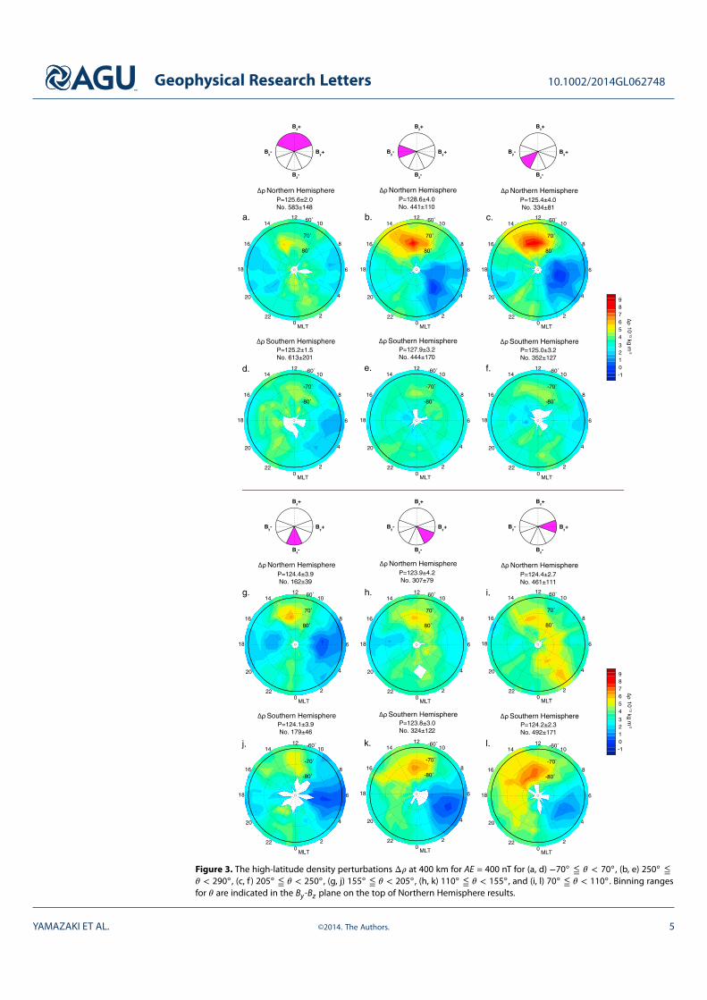
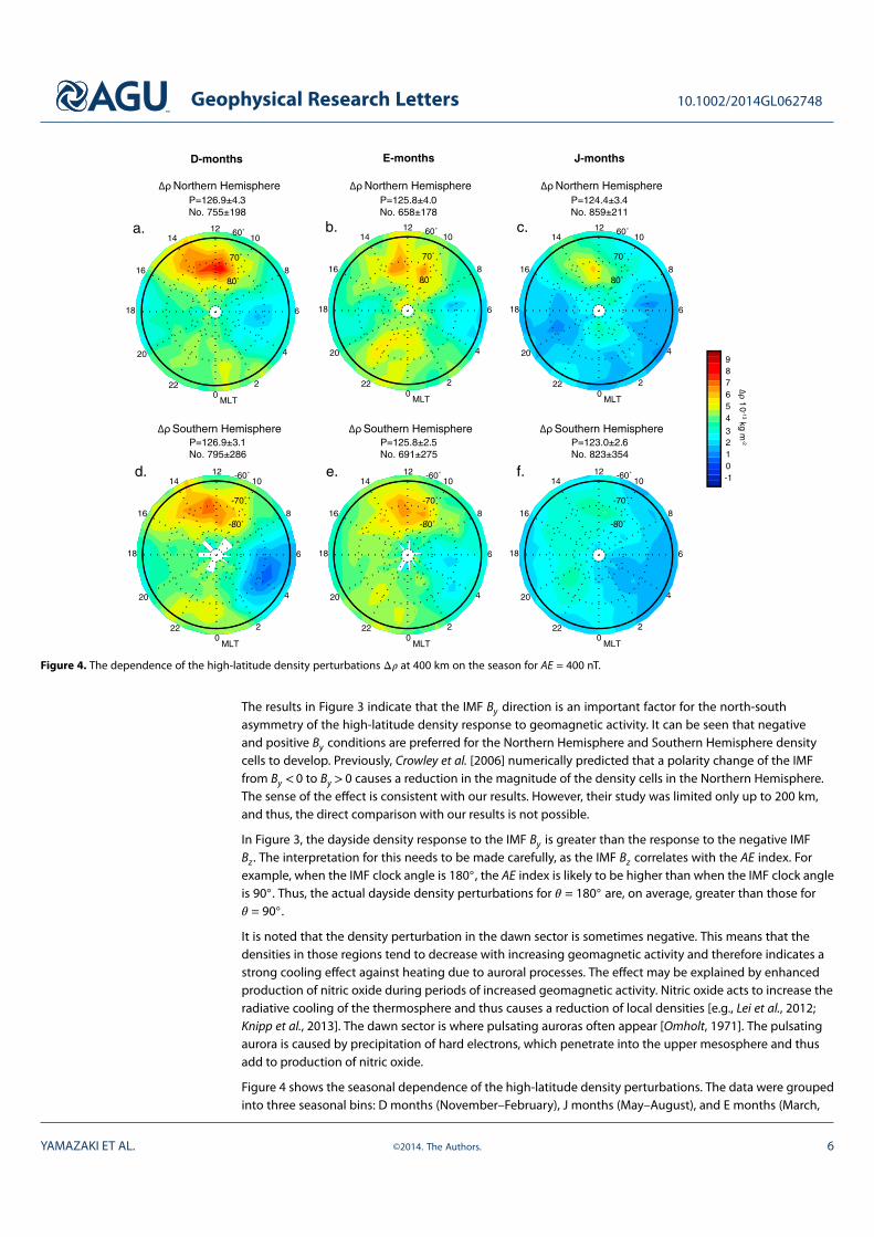
Figure 4. The dependence of the high-latitude density perturbations $! at 400 km on the season for AE = 400 nT.

The results in Figure 3 indicate that the IMF By direction is an important factor for the north-southasymmetry of the high-latitude density response to geomagnetic activity. It can be seen that negativeand positive By conditions are preferred for the Northern Hemisphere and Southern Hemisphere densitycells to develop. Previously, Crowley et al. [2006] numerically predicted that a polarity change of the IMFfrom By <0 to By >0 causes a reduction in the magnitude of the density cells in the Northern Hemisphere.The sense of the e!ect is consistent with our results. However, their study was limited only up to 200 km,and thus, the direct comparison with our results is not possible.

In Figure 3, the dayside density response to the IMF By is greater than the response to the negative IMFBz . The interpretation for this needs to be made carefully, as the IMF Bz correlates with the AE index. Forexample, when the IMF clock angle is 180!, the AE index is likely to be higher than when the IMF clock angleis 90!. Thus, the actual dayside density perturbations for # = 180! are, on average, greater than those for# = 90!.

It is noted that the density perturbation in the dawn sector is sometimes negative. This means that thedensities in those regions tend to decrease with increasing geomagnetic activity and therefore indicates astrong cooling e!ect against heating due to auroral processes. The e!ect may be explained by enhancedproduction of nitric oxide during periods of increased geomagnetic activity. Nitric oxide acts to increase theradiative cooling of the thermosphere and thus causes a reduction of local densities [e.g., Lei et al., 2012;Knipp et al., 2013]. The dawn sector is where pulsating auroras often appear [Omholt, 1971]. The pulsatingaurora is caused by precipitation of hard electrons, which penetrate into the upper mesosphere and thusadd to production of nitric oxide.

Figure 4 shows the seasonal dependence of the high-latitude density perturbations. The data were groupedinto three seasonal bins: D months (November–February), J months (May–August), and E months (March,

YAMAZAKI ET AL. ©2014. The Authors. 6

Geophysical Research Letters 10.1002/2014GL062748

April, September, and October). The results do not show a strong north-south asymmetry unlike the case fornonzero IMF By conditions.

There is an apparent annual modulation in the density response to geomagnetic activity. That is, the overalldensity perturbations are smaller during the J months than D months for the same level of geomagneticactivity. The background thermospheric density tends to be globally low during the J months [e.g., Qianet al., 2009], which may be a reason for the weak response during the J months. Also, the AE index, whichis based on the Northern Hemisphere magnetometer data, undergoes an annual variation [e.g., Singh et al.,2013], and it may a!ect our results.

4. Summary and Conclusions

Earlier studies have established the role of the IMF By in producing a hemispheric asymmetry of thehigh-latitude ion convection and wind. The e!ect of positive/negative By in the Northern Hemispherehas been found to be similar to the e!ect of negative/positive By in the Southern Hemisphere. We haveinvestigated the possible contribution of the IMF By to the north-south asymmetry of the high-latitudethermospheric density response to geomagnetic activity by using air drag measurements from the CHAMPsatellite. The results of our statistical analysis revealed that such an e!ect does exist.

We have shown that the high-latitude disturbance density structure is often characterized by a high-densityregion around the noon sector and a low-density region in the dawn sector. They have the features of thedensity cells, which has been theoretically predicted but only below 350 km [Crowley et al., 1996, 2006]. Itwas found that the cell structures in the Northern Hemisphere and Southern Hemisphere become moreevident under negative and positive By conditions, respectively. This is qualitatively consistent with simula-tion results by Crowley et al. [2006], although their simulations were limited up to 200 km. Their model useddi!erent patterns of the high-latitude ion convection according to the By input, and thus, changes in thedensity were mainly due to the ion drag e!ect on the neutral wind. The model used by Crowley et al. [2006]was, however, unable to examine the possibility that the IMF By might cause a hemispheric asymmetry inthe energy input from the magnetosphere. For example, magnetohydrodynamic simulations of the coupledsolar wind-magnetosphere-ionosphere system by Tanaka [2001] predicted a hemispheric asymmetry inthe distribution of high-latitude field-aligned currents under nonzero IMF By conditions. Further numericalinvestigations will be necessary to clarify the mechanism for the IMF By e!ect on the thermospheric density.

The IMF By e!ect is not considered in most empirical models of the thermosphere. Our results suggest thatthe IMF By e!ect needs to be taken into account for an accurate description of the density response togeomagnetic activity, especially at high latitudes.

The seasonal e!ect was another possible source for the hemispheric asymmetry. However, we did not findevidence of the seasonal e!ect on the north-south asymmetry of the high-latitude density perturbations. Amore comprehensive study is planned to examine the combined e!ect of the seasons and IMF By , e.g., theseasonal e!ect on the north-south asymmetry due to the IMF By e!ect.

Finally, the results in this paper represent only the average state and do not necessarily agree with individualcases. The large scatter of the data, which was found in the binning process (see Figures 2a and 2b), indicatesthat there are many data points that deviate from the average results. Therefore, it is important to be awareof other sources of variability as well, when interpreting case study results.

ReferencesCousins, E. D. P., and S. G. Shepherd (2010), A dynamical model of high-latitude convection derived from SuperDARN plasma drift

measurements, J. Geophys. Res., 115, A12329, doi:10.1029/2010JA016017.Crowley, G., J. Schoendorf, R. G. Roble, and F. Marcos (1996), Cellular structures in the high-latitude thermosphere, J. Geophys. Res., 101,

211–223.Crowley, G., T. J. Immel, C. L. Hackert, J. Craven, and R. G. Roble (2006), E!ect of IMF BY on thermospheric composition at high and

middle latitudes: 1. Numerical experiments, J. Geophys. Res., 111, A10311, doi:10.1029/2005JA011371.Förster, M., S. Rentz, W. Köhler, H. Liu, and S. E. Haaland (2008), IMF dependence of high-latitude thermospheric wind pattern derived

from CHAMP cross-track measurements, Ann. Geophys., 26, 1581–1595, doi:10.5194/angeo-26-1581-2008.Immel, T. J., J. D. Craven, and L. A. Frank (1997), Influence of IMF By on large-scale decreases of O column density at middle latitudes,

J. Atmos. Terr. Phys., 59, 725–736.Immel, T. J., G. Crowley, C. L. Hackert, J. D. Craven, and R. G. Roble (2006), E!ect of IMF By on thermospheric composition at high and

middle latitudes: 2. Data comparisons, J. Geophys. Res., 111, A10312, doi:10.1029/2005JA011372.

AcknowledgmentsThe Kp index was provided by theGerman Research Center forGeosciences, GFZ (http://www.gfz-potsdam.de/en/home). The MgIIindex was provided by the Instituteof Environmental Physics, Univer-sity of Bremen (http://www.iup.uni-bremen.de/gome/gomemgii.html). The F10.7 index was providedby the Herzberg Institute of Astro-physics. The hourly solar wind datawere obtained from the NASA OMNI-web database (http://omniweb.gsfc.nasa.gov/). The SuperMAG AE indexwas downloaded from the Super-MAG website (http://supermag.jhuapl.edu/). For the ground magnetome-ter data we gratefully acknowledge:Intermagnet; USGS, Je!rey J. Love;CARISMA, Ian Mann; CANMOS; TheS-RAMP Database, K. Yumoto andK. Shiokawa; The SPIDR database;AARI, Oleg Troshichev; The MACCSprogram, M. Engebretson, Geomag-netism Unit of the Geological Surveyof Canada; GIMA; MEASURE, UCLAIGPP, and Florida Institute of Technol-ogy; SAMBA, Eftyhia Zesta; 210 Chain,K. Yumoto; SAMNET, Farideh Honary;The institutes who maintain the IMAGEmagnetometer array, Eija Tanskanen;PENGUIN; AUTUMN, Martin Conners;DTU Space, Jürgen Matzka; South Poleand McMurdo Magnetometer, LouisJ. Lanzarotti and Alan T. Weatherwax;ICESTAR; RAPIDMAG; PENGUIn; BritishArtarctic Survey; McMac, Peter Chi;BGS, Susan Macmillan; PushkovInstitute of Terrestrial Magnetism,Ionosphere and Radio Wave Propa-gation (IZMIRAN); GFZ, Monika Korte;SuperMAG, Jesper W. Gjerloev. Y.Y. andM.J.K. were supported by NERC grantNE/K01207X/1.

The Editor thanks Stanley Solomonand an anonymous reviewer for theirassistance in evaluating this paper.

YAMAZAKI ET AL. ©2014. The Authors. 7

Geophysical Research Letters 10.1002/2014GL062748

Knipp, D., L. Kilcommons, L. Hunt, M. Mlynczak, V. Pilipenko, B. Bowman, Y. Deng, and K. Drake (2013), Thermospheric damping responseto sheath-enhanced geospace storms, Geophys. Res. Lett., 40, 1263–1267, doi:10.1002/grl.50197.

Kwak, Y.-S., A. D. Richmond, Y. Deng, J. M. Forbes, and K.-H. Kim (2009), Dependence of the high-latitude thermospheric densities on theinterplanetary magnetic field, J. Geophys. Res., 114, A05304, doi:10.1029/2008JA013882.

Lei, J., A. G. Burns, J. P. Thayer, W. Wang, M. G. Mlynczak, L. A. Hunt, X. Dou, and E. Sutton (2012), Overcooling in the upper thermosphereduring the recovery phase of the 2003 October storms, J. Geophys. Res., 117, A03314, doi:10.1029/2011JA016994.

Lühr, H., M. Rother, W. Köhler, P. Ritter, and L. Grunwaldt (2004), Thermospheric up-welling in the cusp region: Evidence from CHAMPobservations, Geophys. Res. Lett., 31, L06805, doi:10.1029/2003GL019314.

Newell, P. T., and J. W. Gjerloev (2011), Evaluation of SuperMAG auroral electrojet indices as indicators of substorms and auroral power,J. Geophys. Res., 116, A12211, doi:10.1029/2011JA016779.

Omholt, A. (1971), The Optical Aurora, Springer, New York.Qian, L., and S. C. Solomon (2012), Thermospheric density: An overview of temporal and spatial variations, Space Sci. Rev., 168, 147–173,

doi:10.1007/s11214-011-9810-z.Qian, L., S. C. Solomon, and T. J. Kane (2009), Seasonal variation of thermospheric density and composition, J. Geophys. Res., 114, A01312,

doi:10.1029/2008JA013643.Reigber, C., H. Lühr, and P. Schwintzer (2002), CHAMP mission status, Adv. Space Res., 30, 129–134.Richards, P. G., J. A. Fennelly, and D. G. Torr (1994), EUVAC: A solar EUV Flux Model for aeronomic calculations, J. Geophys. Res., 99(A5),

8981–8992, doi:10.1029/94JA00518.Richmond, A. D. (1995), Ionospheric electrodynamics using magnetic apex coordinates, J. Geomagn. Geoelectr., 47, 191–212.Richmond, A. D., and G. Lu (2000), Upper-atmospheric e!ects of magnetic storms: A brief tutorial, J. Atmos. Sol. Terr. Phys., 62, 1115–1127.Ritter, P., H. Lühr, and E. Doornbos (2010), Substorm-related thermospheric density and wind disturbances derived from CHAMP

observations, Ann. Geophys., 28, 1207–1220, doi:10.5194/angeo-28-1207-2010.Singh, A. K., R. Rawat, and B. M. Pathan (2013), On the UT and seasonal variations of the standard and SuperMAG auroral electrojet

indices, J. Geophys. Res. Space Physics, 118, 5059–5067, doi:10.1002/jgra.50488.Solomon, S. C., L. Qian, L. V. Didkovsky, R. A. Viereck, and T. N. Woods (2011), Causes of low thermospheric density during the 2007–2009

solar minimum, J. Geophys. Res., 116, A00H07, doi:10.1029/2011JA016508.Sutton, E. K. (2008), E!ects of solar disturbances on the thermosphere densities and winds from CHAMP and GRACE satellite

accelerometer data, PhD dissertation, Univ. of Colo., Boulder, Colo.Sutton, E. K., J. M. Forbes, and D. J. Knipp (2009), Rapid response of the thermosphere to variations in Joule heating, J. Geophys. Res., 114,

A04319, doi:10.1029/2008JA013667.Tanaka, T. (2001), Interplanetary magnetic field By and auroral conductance e!ects on high-latitude ionospheric convection patterns,

J. Geophys. Res., 106(A11), 24,505–24,516, doi:10.1029/2001JA900061.Viereck, R., L. Puga, D. McMullin, D. Judge, M. Weber, and W. K. Tobiska (2001), The Mg II index: A proxy for solar EUV, Geophys. Res. Lett.,

28, 1343–1346, doi:10.1029/2000GL012551.Yamazaki, Y., A. D. Richmond, and K. Yumoto (2012), Stratospheric warmings and the geomagnetic lunar tide: 1958–2007, J. Geophys.

Res., 117, A04301, doi:10.1029/2012JA017514.

YAMAZAKI ET AL. ©2014. The Authors. 8