Embed Size (px)
Citation preview
Available online at www.sciencedirect.com
ScienceDirect
J. Differential Equations 257 (2014) 921–1011
www.elsevier.com/locate/jde
Normal forms for semilinear equations with non-densedomain with applications to age structured models
Zhihua Liu a,1, Pierre Magal b,c,d,∗,2, Shigui Ruan e,3
a School of Mathematical Sciences, Beijing Normal University, Beijing 100875, People’s Republic of Chinab Univ. Bordeaux, IMB, UMR 5251, F-33400 Talence, France
c CNRS, IMB, UMR 5251, F-33400 Talence, Franced School of Mathematics, Sichuan University, Chengdu 610064, People’s Republic of China
e Department of Mathematics, University of Miami, Coral Gables, FL 33124-4250, USA
Received 20 June 2013; revised 17 April 2014
Available online 14 May 2014
Abstract
Normal form theory is very important and useful in simplifying the forms of equations restricted onthe center manifolds in studying nonlinear dynamical problems. In this paper, using the center manifoldtheorem associated with the integrated semigroup theory, we develop a normal form theory for semilinearCauchy problems in which the linear operator is not densely defined and is not a Hille–Yosida operator andpresent procedures to compute the Taylor expansion and normal form of the reduced system restricted onthe center manifold. We then apply the main results and computation procedures to determine the direc-tion of the Hopf bifurcation and stability of the bifurcating periodic solutions in a structured evolutionaryepidemiological model of influenza A drift and an age structured population model.© 2014 Elsevier Inc. All rights reserved.
MSC: 37L10; 37G05; 34K18; 34C20; 58B32
Keywords: Normal form; Non-densely defined Cauchy problem; Center manifold; Hopf bifurcation; Structuredpopulation; Population dynamics
* Corresponding author.1 Research was partially supported by National Natural Science Foundation of China (NNSFC), grant Nr. 11371058.2 Research was partially supported by the French Ministry of Foreign and European Affairs program France–China
PFCC Campus France (20932UL).3 Research was partially supported by National Science Foundation (DMS-1022728).
http://dx.doi.org/10.1016/j.jde.2014.04.0180022-0396/© 2014 Elsevier Inc. All rights reserved.
922 Z. Liu et al. / J. Differential Equations 257 (2014) 921–1011
Contents
1. Introduction . . . . . . . . . . . . . . . . . . . . . . . . . . . . . . . . . . . . . . . . . . . . . . . . . . . . . . . 9221.1. Normal form theory . . . . . . . . . . . . . . . . . . . . . . . . . . . . . . . . . . . . . . . . . . . . . 9221.2. Motivation – age structured models . . . . . . . . . . . . . . . . . . . . . . . . . . . . . . . . . . . 9231.3. Nonlinear dynamics of semilinear equations with non-dense domain . . . . . . . . . . . . 9261.4. An outline . . . . . . . . . . . . . . . . . . . . . . . . . . . . . . . . . . . . . . . . . . . . . . . . . . . . 927
2. Preliminaries and the sketchy computation procedure . . . . . . . . . . . . . . . . . . . . . . . . . . . 9272.1. Semiflows generated by nondensely defined Cauchy problems . . . . . . . . . . . . . . . . 9272.2. Spectral decomposition of the state space . . . . . . . . . . . . . . . . . . . . . . . . . . . . . . . 9292.3. Center manifold theorem . . . . . . . . . . . . . . . . . . . . . . . . . . . . . . . . . . . . . . . . . . 9322.4. A sketchy procedure of computing the reduced system . . . . . . . . . . . . . . . . . . . . . . 933
3. Normal form theory – nonresonant type results . . . . . . . . . . . . . . . . . . . . . . . . . . . . . . . . 9363.1. G ∈ V m(Xc,D(A) ∩ Xh) . . . . . . . . . . . . . . . . . . . . . . . . . . . . . . . . . . . . . . . . . 9373.2. G ∈ V m(Xc,D(A)) . . . . . . . . . . . . . . . . . . . . . . . . . . . . . . . . . . . . . . . . . . . . . 945
4. Normal form computation . . . . . . . . . . . . . . . . . . . . . . . . . . . . . . . . . . . . . . . . . . . . . . 9494.1. G ∈ V m(Xc,D(A) ∩ Xh) . . . . . . . . . . . . . . . . . . . . . . . . . . . . . . . . . . . . . . . . . 9494.2. G ∈ V m(Xc,D(A)) . . . . . . . . . . . . . . . . . . . . . . . . . . . . . . . . . . . . . . . . . . . . . 952
5. Applications . . . . . . . . . . . . . . . . . . . . . . . . . . . . . . . . . . . . . . . . . . . . . . . . . . . . . . . 9555.1. A structured model of influenza A drift . . . . . . . . . . . . . . . . . . . . . . . . . . . . . . . . 9555.2. An age structured population model . . . . . . . . . . . . . . . . . . . . . . . . . . . . . . . . . . 991
References . . . . . . . . . . . . . . . . . . . . . . . . . . . . . . . . . . . . . . . . . . . . . . . . . . . . . . . . . . . . . 1009
1. Introduction
1.1. Normal form theory
To determine the qualitative behavior of a nonlinear system in the neighborhood of a nonhy-perbolic equilibrium point, the center manifold theorem implies that it could be reduced to theproblem of determining the qualitative behavior of the nonlinear system restricted on the centermanifold, which reduces the dimension of a local bifurcation problem near the nonhyperbolicequilibrium point. The normal form theory provides a way of finding a nonlinear analytic trans-formation of coordinates in which the nonlinear system restricted on the center manifold takesthe “simplest” form, called normal form. These two methods, one reduces the dimension of theoriginal system and the other eliminates the nonlinearity of the reduced system, are conjunctlyused to study bifurcations in nonlinear dynamical systems. A normal form theorem was obtainedfirst by Poincaré [54] and later by Siegel [56] for analytic differential equations. Simpler proofsof Poincaré’s theorem and Siegel’s theorem were given in Arnold [5], Meyer [46], Moser [48],and Zehnder [67]. For more results about normal form theory and its applications see, for exam-ple, the monographs by Arnold [5], Chow and Hale [8], Guckenheimer and Holmes [26], Meyerand Hall [47], Siegel and Moser [57], Chow et al. [9], Kuznetsov [34], and others.
Normal form theory has been extended to various classes of partial differential equations. Inthe context of autonomous partial differential equations we refer to Ashwin and Mei [6] (PDEson the square), Eckmann et al. [18] (abstract parabolic equations), Faou et al. [20,21] (Hamilto-nian PDEs), Hassard, Kazarinoff and Wan [28] (functional differential equations), Faria [22,23](PDEs with delay), Foias et al. [25] (Navier–Stokes equation), Kokubu [33] (reaction–diffusion

Z. Liu et al. / J. Differential Equations 257 (2014) 921–1011 923
equations), McKean and Shatah [45] (Schrödinger equation and heat equations), Nikolenko [51](abstract semi-linear equations), Shatah [55] (Klein–Gordon equation), Zehnder [68] (abstractparabolic equations), etc. We refer to Chow et al. [10] (and references therein) for a normal formtheory in quasiperiodic partial differential equations.
In this paper, we develop a normal form theory for the following abstract Cauchy problemwith non-dense domain ⎧⎨⎩
du(t)
dt= Au(t) + F
(u(t)
), t ≥ 0,
u(0) = x ∈ D(A),
(1.1)
where A : D(A) ⊂ X → X is a non-densely defined linear operator on a Banach space X, andF : D(A) → X is a k-time continuously differentiable function for some k ≥ 2. The Cauchyproblem (1.1) is said to be non-densely defined if
D(A) �= X.
Therefore A is not the infinitesimal generator of a strongly continuous semigroup of bounded lin-ear operators on X, and in general, F(x) does not belong to D(A). So the solution of system (1.1)is not a mild solution derived from the classical semi-linear formulation.
1.2. Motivation – age structured models
The main motivation comes from investigating the nonlinear dynamics of structured (age,size, space, etc.) population models described by various types of equations including par-tial differential equations with nonlinear and nonlocal boundary conditions (Cantrell and Cos-ner [7], Diekmann and Heesterbeek [14], Iannelli [29], Magal and Ruan [41], Murray [49],Perthame [53], Thieme [61], Webb [64], etc.). It is well-known that several types of differentialequations, such as functional differential equations (Adimy [1], Diekmann et al. [15], Hale andVerduyn Lunel [27], Liu et al. [35]), age structured models (Magal [39], Magal and Ruan [42],Perthame [53], Thieme [58,60], and Webb [64]), parabolic partial differential equations (Chuet al. [11], Ducrot et al. [16]), and partial differential equations with delay (Ducrot et al. [17]and Wu [66]), can be formulated as non-densely defined Cauchy problems in the form of (1.1).Here we present two examples of structured models and refer to Da Prato and Sinestrari [13],Thieme [58,59], and Magal and Ruan [40,42] for more examples.
(a) A structured model of influenza A drift. Suppose that the total host population size N
is a constant. Let I (t) be the number of infected individuals at time t . Let a ≥ 0 be the timesince the last infection, that is, the duration of time since an individual has been susceptible.Assume that the average number of amino acid substitutions is a continuous variable. Moreprecisely, let k > 0 be the average number of amino acid substitutions per unit of time (that is,the mutation rate). Then the number of substitutions after a period of time a in the susceptibleclass is given by ka. Let s(t, a) be the density of uninfected hosts (structured with respect to a),so that
∫ a1a0
s(t, a)da = ∫ ka1ka0
s(t, k−1l)k−1dl is the number of uninfected hosts that were lastinfected by a virus which differed by more than ka0 and less than ka1 amino acid substitutionsfrom the virus strain prevailing at time t . ν > 0 is the recovery rate of the infected hosts. γ ∈L∞+ (0,+∞) describes how amino acid substitutions affect the probability of reinfection and

924 Z. Liu et al. / J. Differential Equations 257 (2014) 921–1011
satisfies lim infa→+∞ γ (ka) > 0. Define ρ := τ/k as the threshold of sensitivity, which is thetime necessary to be re-infected after one infection. This is also equivalent to assuming that it isnecessary to reach a threshold value τ for the average number of amino acid substitutions beforere-infection. Assume that
γ (a) = δχ(a) :={
δ if a ≥ τ,
0 if a ∈ (0, τ ),
where δ > 0. Note that∫ +∞
0 s(t, a)(a)da + I (t) = N , ∀t ≥ 0. Assume without loss of gener-ality that k = 1 and N = 1. Then we have a structured evolutionary epidemiological model ofinfluenza A drift (see Pease [52], Inaba [30,31], Magal and Ruan [44])⎧⎪⎪⎪⎪⎪⎪⎪⎪⎪⎪⎪⎪⎪⎪⎨⎪⎪⎪⎪⎪⎪⎪⎪⎪⎪⎪⎪⎪⎪⎩
∂s(t, a)
∂t+ ∂s(t, a)
∂a= −δχ(a)s(t, a)
(1 −
+∞∫0
s(t, l)dl
)+, t ≥ 0, a ≥ 0,
s(t, 0) = ν
(1 −
+∞∫0
s(t, l)dl
)+,
s(0, .) = s0 ∈ L1+(0,+∞) with
+∞∫0
s0(l)dl ≤ 1,
(1.2)
where x+ = max(x, 0). Consider the Banach space
X =R× L1(0,+∞)
endowed with the usual product norm∥∥∥∥(α
ϕ
)∥∥∥∥= |α| + ‖ϕ‖L1 .
Consider the linear operator A : D(A) ⊂ X → X defined by
A
(0
ϕ
)=(−ϕ(0)
−ϕ′
)(1.3)
with
D(A) = {0} × W 1,1(0,+∞).
Then
X0 := D(A) = {0} × L1(0,+∞).
Set
X+ := R+ × L1 (0,+∞) and X0+ := X0 ∩ X+ = {0} × L1 (0,+∞).
+ +
Z. Liu et al. / J. Differential Equations 257 (2014) 921–1011 925
We also consider the nonlinear operator F : (0,+∞) × (0,+∞) × D(A) → X defined by
F
(ν, δ,
(0
ϕ
))=(
ν(1 − ∫ +∞0 ϕ(l)dl)+
−(1 − ∫ +∞0 ϕ(l)dl)+δχϕ
). (1.4)
By identifying s(t, .) with u(t) =(
0
s(t,.)
), we can rewrite the system as the following abstract
Cauchy problem
du(t)
dt= Au(t) + F
(ν, δ, u(t)
)for t ≥ 0 and u(0) =
(0
s0
)∈ D(A). (1.5)
(b) An age structured population model. Let u(t, a) denote the density of a population at timet with age a. Consider the following age structured model with nonlinear boundary conditions(see Magal and Ruan [43])⎧⎪⎪⎪⎪⎪⎪⎪⎨⎪⎪⎪⎪⎪⎪⎪⎩
∂u(t, a)
∂t+ ∂u(t, a)
∂a= −μu(t, a), a ∈ (0,+∞),
u(t, 0) = αh
( +∞∫0
γ (a)u(t, a)da
),
u(0, .) = ϕ ∈ L1+((0,+∞);R),
(1.6)
where μ > 0 is the mortality rate of the population, αγ (a) is the fertility rate at age a, α ≥ 0 isa parameter, the function h(·) describes some limitation for the reproduction of the population.Similarly as in (a) for Eq. (1.2), consider the same space X = R × L1(0,+∞) with the usualproduct norm. Let A : D(A) ⊂ X → X be the linear operator on X defined by
A
(0
ϕ
)=( −ϕ(0)
−ϕ′ − μϕ
)(1.7)
with the same domain D(A) = {0} × W 1,1(0,+∞) and D(A) = X0. Let H : X0 → X be themap defined by
H
((0
ϕ
))=(
h(∫ +∞
0 γ (a)ϕ(a)da)
0L1
). (1.8)
Then by identifying u(t, .) to v(t) =(
0
u(t,.)
)∈ X0, the system (1.6) can be reformulated as the
following non-densely defined abstract Cauchy problem
dv(t)
dt= Av(t) + αH
(v(t)
), for t ≥ 0, v(0) =
(0
ϕ0
)∈ D(A). (1.9)
It has been shown that Hopf bifurcation can occur in age-structured models such as (1.2)and (1.6) (see Magal and Ruan [44,43] and references cited therein) and a Hopf bifurcationtheory has been recently developed for general age structured models in Liu et al. [36]. But up to
926 Z. Liu et al. / J. Differential Equations 257 (2014) 921–1011
now, the stability of the bifurcating periodic orbits is unknown for such systems. To address thisissue, a normal form theory for age structured models, and more generally for the non-denselydefined abstract Cauchy problem, needs to be developed. This is a first motivation for this paper.Another motivation is coming from the analysis of Bogdanov–Takens bifurcation in the contextof age structured models. By using the normal theory presented in this article Liu, Magal andXiao [38] obtain recently a first example of Bogdanov–Takens for an age structured model.
1.3. Nonlinear dynamics of semilinear equations with non-dense domain
For the semilinear Cauchy problem (1.1), if A is a Hille–Yosida operator and is densely de-fined (i.e., D(A) = X), given an initial datum in the phase space integrating the equation yieldsa corresponding trajectory through that point (the constant of variation formula), so the semilin-ear Cauchy problem is well-posed and has been extensively studied, see Engel and Nagel [19].When A is non-densely defined (i.e., D(A) �= X), the constant of variation formula may be notwell-defined and one may be able to integrate the equation twice to recover the well-posedness(this is how integrated semigroups are introduced). When A is a Hille–Yosida operator but itsdomain is non-densely defined, Da Prato and Sinestrari [13] investigated the existence of severaltypes of solutions for non-densely defined Cauchy problems. Thieme [58] studied the semilinearCauchy problem with a Lipschitz perturbation of the closed linear operator A by using integratedsemigroup theory.
We have been interested in studying the nonlinear dynamics, such as stability, bifurcations,periodic solutions, and invariant manifolds, in the semilinear Cauchy problem (1.1) when A isnon-densely defined and is not Hille–Yosida, and have made some progress on this subject. Ma-gal and Ruan [40] presented some techniques and results for integrated semigroups, obtainednecessary and sufficient conditions for the existence of mild solutions for non-densely definednon-homogeneous Cauchy problems, and applied the results to study age-structured models. Ma-gal and Ruan [42] extended the results of Thieme [58] to the case when the operator A is notHille–Yosida. Namely, we studied the positivity of solutions to the semilinear problem (1.1),the Lipschitz perturbation of the problem, differentiability of the solutions with respect to thestate variable, time differentiability of the solutions, and the stability of equilibria. Magal andRuan [43] established a center manifold theory for the semilinear Cauchy problem (1.1) withnon-dense domain. Center-unstable manifolds for non-densely defined semilinear Cauchy prob-lems were studied in Liu et al. [37]. Employing the center manifold theory in [43], Liu et al. [36]established a Hopf bifurcation theorem for abstract non-densely defined Cauchy problems.
In this paper we use the integrated semigroup theory, the semilinear Cauchy problem the-ory, and the center manifold theory (see [40,42,43]) to establish a normal form theory for thenon-densely defined Cauchy problem (1.1) when D(A) is not dense in X and A is not a Hille–Yosida operator. The goal is to provide a method for computing the required lower order terms ofthe Taylor expansion and the normal form of the reduced equations. The main difficulty comesfrom the fact that the center manifold is defined by using implicit formulae in general. Here wewill show that it is possible to find some appropriate changes of variables (in Banach spaces)to compute the Taylor expansion at any order and the normal form of the reduced system. Themain results and computation procedures will be used to Hopf bifurcation in the structured evo-lutionary epidemiological model of influenza A drift (1.2) and the age structured populationmodel (2.2).
Z. Liu et al. / J. Differential Equations 257 (2014) 921–1011 927
1.4. An outline
The plan of the paper is as follows. In Section 2, we will present some preliminary resultson integrated semigroups and the center manifold theorem for the non-densely defined Cauchyproblem (1.1) and give an outline on the computation of the reduced system restricted on thecenter manifold. In Section 3, we introduce some notions, justify the change of variables thatestablishes the equivalence between the original and reduced systems and present the normalform theory of the nonresonance type. In Section 4, we provide computational procedures forthe Taylor expansion and normal form of the reduced system on the center manifold. Section 5is devoted to the application of the normal theory to the two structured models (1.2) and (1.6);namely, we calculate the Taylor expansion of the reduced system of the structured evolutionaryepidemiological model (1.2) of influenza A drift on the center manifold and present the normalform of the age structured population model (1.6) restricted on the center manifold, respectively,from which we are able to study stability and direction of the Hopf bifurcation in these twostructured models.
2. Preliminaries and the sketchy computation procedure
2.1. Semiflows generated by nondensely defined Cauchy problems
A mild solution of Eq. (1.1) (or integrated solution) is a solution of the integral equation
u(t) = x + A
t∫0
u(s)ds +t∫
0
F(u(s)
)ds for each t ≥ 0,
wherein
t∫0
u(s)ds ∈ D(A) for each t ≥ 0.
This last inclusion implies in particular that u(t) ∈ D(A) for each t ≥ 0.From hereon, set
X0 := D(A)
and consider A0 as the part of A in X0. That is, A0 is the linear operator on X0 defined by
A0 = A on D(A0) := {x ∈ D(A) : Ax ∈ X0}.
Throughout this article, we will make the following assumption:
Assumption 2.1. We assume that:
(i) The resolvent set ρ(A) of A is non-empty;(ii) A0 is the infinitesimal generator of a strongly continuous semigroup {TA0(t)}t≥0 of bounded
linear operators on X0.
928 Z. Liu et al. / J. Differential Equations 257 (2014) 921–1011
Since ρ(A) is non-empty, we have ρ(A) = ρ(A0) and can define the integrated semigroup{SA(t)}t≥0 ⊂ L(X) generated by A as
SA(t) := (λI − A0)
t∫0
TA0(s)ds(λI − A)−1
whenever λ ∈ ρ(A). Then it is equivalent to considering a mild solution or a solution of
u(t) = TA0(t)x + (SA � F(u))(t) for t ≥ 0,
where
(SA � f )(t) := d
dt(SA ∗ f )(t),
whenever t → (SA ∗ f )(t) := ∫ t
0 SA(t − s)f (s)ds is differentiable.We refer to Arendt [2,3], Arendt et al. [4], Da Prato and Sinestrari [13], Kellermann and
Hieber [32], Magal and Ruan [40,43], Neubrander [50], and Thieme [59,60] for more results andreferences on integrated semigroups. When A is a Hille–Yosida operator (see Kellermann andHieber [32]), the convolution (SA ∗ f )(t) is differentiable with respect to the time variable t aslong as f ∈ L1((0, τ ),X) (with τ < +∞), and one has the following estimation
∥∥(SA � f )(t)∥∥≤ M
t∫0
eω(t−s)∥∥f (s)
∥∥ds, ∀t ≥ 0,
for some constant M ≥ 1, and ω ∈R.For the age structured model (1.2), the linear operator A is Hille–Yosida if and only if p = 1.
When p > 1, the time differentiability of (SA ∗ f )(t) becomes more difficult. Similar difficul-ties arise in the context of parabolic equations with nonhomogeneous boundary conditions (seeDucrot et al. [16]). Therefore, here we will consider the most general case in which A is not aHille–Yosida operator. In this case, the time differentiability of (SA ∗ f )(t) becomes an issue.In practice, this question is related to the existence of solutions for PDE problems with nonho-mogeneous boundary conditions which are only Lp integrable in time. This question has beenstudied recently in Magal and Ruan [40] and Thieme [60] for the general case and in [16] for thealmost sectorial case.
Motivated by the above discussions, in this paper we will make the following assumption.
Assumption 2.2. The map t → (SA ∗ f )(t) is differentiable whenever t → f (t) is continuous,and there exists a map δ : [0,+∞) → [0,+∞) such that∥∥(SA � f )(t)
∥∥≤ δ(t) sups∈[0,t]
∥∥f (s)∥∥, ∀t ≥ 0,
where
δ(t) → 0 as t ↘ 0.
Z. Liu et al. / J. Differential Equations 257 (2014) 921–1011 929
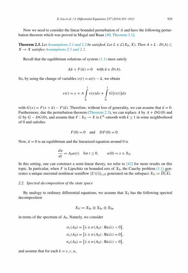
Now we need to consider the linear bounded perturbation of A and have the following pertur-bation theorem which was proved in Magal and Ruan [40, Theorem 3.1].
Theorem 2.3. Let Assumptions 2.1 and 2.2 be satisfied. Let L ∈ L(X0,X). Then A+L : D(A) ⊂X → X satisfies Assumptions 2.1 and 2.2.
Recall that the equilibrium solutions of system (1.1) must satisfy
Au + F(u) = 0 with u ∈ D(A).
So, by using the change of variables v(t) = u(t) − u, we obtain
v(t) = x + A
t∫0
v(s)ds +t∫
0
G(v(t)
)ds
with G(x) = F(x + u) − F(u). Therefore, without loss of generality, we can assume that u = 0.Furthermore, due the perturbation theorem (Theorem 2.3), we can replace A by A + DG(0) andG by G − DG(0), and assume that F : X0 → X is Ck-smooth with k ≥ 1 in some neighborhoodof 0 and satisfies
F(0) = 0 and DF(0) = 0.
Now, u = 0 is an equilibrium and the linearized equation around 0 is
du
dt= A0u(t) for t ≥ 0, u(0) = x ∈ X0.
In this setting, one can construct a semi-linear theory, we refer to [42] for more results on thistopic. In particular, when F is Lipschitz on bounded sets of X0, the Cauchy problem (1.1) gen-erates a unique maximal nonlinear semiflow {U(t)}t≥0 generated on the subspace X0 := D(A).
2.2. Spectral decomposition of the state space
By analogy to ordinary differential equations, we assume that X0 has the following spectraldecomposition
X0 := X0s ⊕ X0c ⊕ X0u
in terms of the spectrum of A0. Namely, we consider
σs(A0) = {λ ∈ σ(A0) : Re(λ) < 0},
σc(A0) = {λ ∈ σ(A0) : Re(λ) = 0},
σu(A0) = {λ ∈ σ(A0) : Re(λ) > 0},
and assume that for each k = s, c, u,
930 Z. Liu et al. / J. Differential Equations 257 (2014) 921–1011
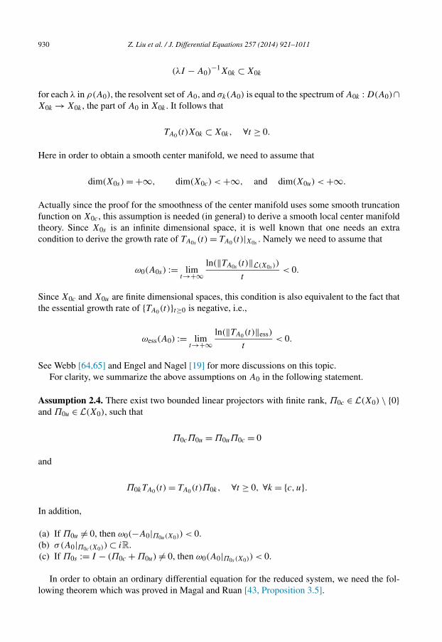
(λI − A0)−1X0k ⊂ X0k
for each λ in ρ(A0), the resolvent set of A0, and σk(A0) is equal to the spectrum of A0k : D(A0)∩X0k → X0k , the part of A0 in X0k . It follows that
TA0(t)X0k ⊂ X0k, ∀t ≥ 0.
Here in order to obtain a smooth center manifold, we need to assume that
dim(X0s) = +∞, dim(X0c) < +∞, and dim(X0u) < +∞.
Actually since the proof for the smoothness of the center manifold uses some smooth truncationfunction on X0c , this assumption is needed (in general) to derive a smooth local center manifoldtheory. Since X0s is an infinite dimensional space, it is well known that one needs an extracondition to derive the growth rate of TA0s
(t) = TA0(t)|X0s. Namely we need to assume that
ω0(A0s) := limt→+∞
ln(‖TA0s(t)‖L(X0s ))
t< 0.
Since X0c and X0u are finite dimensional spaces, this condition is also equivalent to the fact thatthe essential growth rate of {TA0(t)}t≥0 is negative, i.e.,
ωess(A0) := limt→+∞
ln(‖TA0(t)‖ess)
t< 0.
See Webb [64,65] and Engel and Nagel [19] for more discussions on this topic.For clarity, we summarize the above assumptions on A0 in the following statement.
Assumption 2.4. There exist two bounded linear projectors with finite rank, Π0c ∈ L(X0) \ {0}and Π0u ∈ L(X0), such that
Π0cΠ0u = Π0uΠ0c = 0
and
Π0kTA0(t) = TA0(t)Π0k, ∀t ≥ 0, ∀k = {c,u}.
In addition,
(a) If Π0u �= 0, then ω0(−A0|Π0u(X0)) < 0.(b) σ(A0|Π0c(X0)) ⊂ iR.(c) If Π0s := I − (Π0c + Π0u) �= 0, then ω0(A0|Π0s (X0)) < 0.
In order to obtain an ordinary differential equation for the reduced system, we need the fol-lowing theorem which was proved in Magal and Ruan [43, Proposition 3.5].

Z. Liu et al. / J. Differential Equations 257 (2014) 921–1011 931
Theorem 2.5. Let Assumption 2.1 be satisfied. Let Π0 : X0 → X0 be a bounded linear operatorof projection satisfying the following properties
Π0(λI − A0)−1 = (λI − A0)−1Π0, ∀λ > ω,
and
Π0(X0) ⊂ D(A0) and A0|Π0(X0) is bounded.
Then there exists a unique bounded linear operator of projection Π on X satisfying the followingproperties:
(i) Π |X0 = Π0.(ii) Π(X) ⊂ X0.
(iii) Π(λI − A)−1 = (λI − A)−1Π , ∀λ > ω.
Since dim(X0c) < +∞ and dim(X0u) < +∞, the linear operators A0c and A0u are bounded.So we can apply the above theorem to obtain Πc (respectively Πu), a unique extension of theprojectors on Π0c (respectively Π0u). Define
Πs := I − (Πc + Πu).
Then we obtain a decomposition of the larger state space
X = Xs ⊕ Xc ⊕ Xu
with
Xc = X0c, Xu = X0u, X0s � Xs,
and such that
(λI − A)−1Xk ⊂ Xk, ∀λ ∈ ρ(A).
Moreover, for k = s, c, u, we have σ(Ak) = σk(A0), wherein Ak is the part of A in Xk .Now, for k = c,u, we can project (1.1) on X0k , and uk(t) := Πku(t) satisfies an ordinary
differential equation
duk(t)
dt= Akuk(0) + ΠkF
(u(t)
)while when we project (1.1) on X0s , us(t) = Πsu(t) is a solution of a new non-densely definedCauchy problem on Xs :
dus(t) = Asus(0) + ΠsF(u(t)
).
dt

932 Z. Liu et al. / J. Differential Equations 257 (2014) 921–1011
At this level, in order to construct a comprehensive center manifold theory, one needs an eval-uation of ‖Πs(SA � F(u))(t)‖ = ‖(SAs � ΠsF(u))(t)‖ expressed as a function of the growthrate of TA0s
(t) = TA0(t)|X0s. So the following result which was proved in Magal and Ruan [42,
Proposition 2.14] plays a particularly important role in this context.
Proposition 2.6. Let Assumptions 2.1 and 2.2 be satisfied. Let ωA ∈ R and MA ≥ 1 be such that∥∥TA(t)∥∥≤ MAeωAt , ∀t ≥ 0.
Let ε > 0 be fixed. Then for each τε > 0 satisfying MAδ(τε) ≤ ε, we have∥∥(SA � f )(t)∥∥≤ C(ε, γ ) sup
s∈[0,t]eγ (t−s)
∥∥f (s)∥∥, ∀t ≥ 0,
whenever γ ∈ (ωA,+∞), f ∈ C(R+,X), and with
C(ε, γ ) := 2ε max(1, e−γ τε )
1 − e(ωA−γ )τε.
2.3. Center manifold theorem
Set
Xh := Xs ⊕ Xu.
Let Πc ∈ L(X) be the projector satisfying
Πc(X) = Xc and (I − Πc)(X) = Xh.
Define
Πh := I − Πc.
The following result is based on the approach developed by Vanderbauwhede [62] and Vander-bauwhede and Iooss [63, Theorem 3]. In the context of integrated semigroups the following resultwas proved in Magal and Ruan [43, Theorem 4.21].
Theorem 2.7. Let Assumptions 2.1, 2.2 and 2.4 be satisfied. Let r > 0 and let F : BX0(0, r) → X
be a map. Assume that there exists an integer k ≥ 1 such that F is k-time continuously differen-tiable in BX0(0, r) with F(0) = 0 and DF(0) = 0. Assume that F : X0 → X is Ck-smooth withk ≥ 1 in some neighborhood of 0. Then in the setting described above, there exists a Ck-smoothfunction Ψ : X0c → X0h which satisfies Ψ (0) = 0, DΨ (0) = 0, and
M = {xc + Ψ (xc) : xc ∈ X}
(center manifold)
is a locally invariant center manifold for the semiflow generated by (1.1). This means that thereexists Ω ⊂ X0, a bounded neighborhood of 0 in X0, such that

Z. Liu et al. / J. Differential Equations 257 (2014) 921–1011 933
if u(0) ∈ M ∩ Ω and u(t) ∈ Ω, ∀t ∈ [0, τ ], then u(t) ∈ M.
Moreover, as Πc is defined on X, we can project (1.1) on Xc and obtain an ordinary differentialequation
duc(t)
dt= A0cuc(t) + ΠcF
[uc(t) + Ψ
(uc(t)
)](reduced system). (2.1)
Furthermore, if t → uc(t) is a solution on an interval I of the reduced system (2.1) and
uc(t) + Ψ(uc(t)
) ∈ Ω, ∀t ∈ I,
then t → u(t) := uc(t) + Ψ (uc(t)) is a mild solution of system (1.1); namely,
u(t) = u(s) + A
t∫s
u(l)dl +t∫
s
F(u(s)
)ds, ∀t, s ∈ I with t ≥ s.
Conversely, if u :R→ X0 is a complete orbit of (1.1) and if
u(t) ∈ Ω, ∀t ∈ R,
then
u(t) ∈ M, ∀t ∈ R,
and t → Πcu(t) is a solution of the reduced system (2.1).
2.4. A sketchy procedure of computing the reduced system
Our paper is devoted to the computation of the Taylor expansion and normal form of thereduced system (2.1). First, one needs to realize that the center manifold Ψ is known only throughan implicit fixed point procedure. Of course, when
DlΨ (0) = 0 for each l = 1, . . . , k,
the Taylor expansion of the reduced system (2.1) is simply given by
duc(t)
dt= A0cuc(t) +
k∑l=1
1
l!ΠcDlF (0)
(uc(t), . . . , uc(t)
)+ h.o.t.
In general, the only information available to compute the Taylor expansion and normal form ofthe reduced system is the following result (see Magal and Ruan [43, Lemma 4.20]).

934 Z. Liu et al. / J. Differential Equations 257 (2014) 921–1011
Lemma 2.8. Let Assumptions 2.1, 2.2 and 2.4 be satisfied. Let r > 0 and let F : BX0(0, r) → X
be a k-time continuously differentiable map (with k ≥ 1) in BX0(0, r) with
F(0) = 0 and DF(0) = 0
and
ΠhDj F(0)|Xc×Xc×···×Xc = 0 for each j = 2, . . . , k.
Then
Dj Ψ (0) = 0 for each j = 1, . . . , k.
Description of the method at the order 3. Assume first that
ΠhD2F(0)|Xc×Xc �= 0.
Let G ∈ V 2(Xc,D(A) ∩ Xh) be a homogeneous polynomial of degree 2 (see Section 3 for aprecise definition). Consider the following global change of variable
v := u − G(Πcu) ⇔{
Πcv = Πcu,
Πhv = Πhu − G(Πcu)⇔ u = v + G(Πcv). (2.2)
Then formally (since the solution is not time differentiable), we obtain
v′ = u′ − DG(Πcu)(Πcu
′)= Au + F(u) − DG(Πcu)
(Πc
[Au + F(u)
]).
Thus
v′ = A[v + G(Πcv)
]+ F(v + G(Πcv)
)− DG(Πcv)
(Πc
[Av + F
(v + G(Πcv)
)]).
We naturally introduce the Lie bracket
[A,G](xc) = DG(xc)(Acxc) − AG(xc), ∀xc ∈ Xc.
Then we obtain a new non-densely defined Cauchy problem
dv(t)
dt= Av(t) + H
(v(t)
)for t ≥ 0 and v(0) = x ∈ D(A), (2.3)
where
H(v) = F[v + G(Πcv)
]− [A,G](Πcv) − DG(Πcv)(ΠcF
(v + G(Πcv)
)).
Z. Liu et al. / J. Differential Equations 257 (2014) 921–1011 935
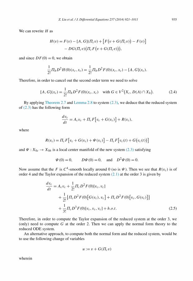
We can rewrite H as
H(v) = F(v) − [A,G](Πcv) + [F (v + G(Πcv))− F(v)
]− DG(Πcv)
(ΠcF
(v + G(Πcv)
)),
and since DF(0) = 0, we obtain
1
2!ΠhD2H(0)(xc, xc) = 1
2!ΠhD2F(0)(xc, xc) − [A,G](xc).
Therefore, in order to cancel out the second order term we need to solve
[A,G](xc) = 1
2!ΠhD2F(0)(xc, xc) with G ∈ V 2(Xc,D(A) ∩ Xh
). (2.4)
By applying Theorem 2.7 and Lemma 2.8 to system (2.3), we deduce that the reduced systemof (2.3) has the following form
dvc
dt= Acvc + ΠcF
[vc + G(vc)
]+ R(vc),
where
R(vc) = ΠcF[vc + G(vc) + Ψ (vc)
]− ΠcF[vc(t) + G
(vc(t)
)]and Ψ : X0c → X0h is a local center manifold of the new system (2.3) satisfying
Ψ (0) = 0, DΨ (0) = 0, and D2Ψ (0) = 0.
Now assume that the F is C4-smooth locally around 0 (so is Ψ ). Then we see that R(vc) is oforder 4 and the Taylor expansion of the reduced system (2.1) at the order 3 is given by
dvc
dt= Acvc + 1
2!ΠcD2F(0)[vc, vc]
+ 1
2!{ΠcD
2F(0)[G(vc), vc
]+ ΠcD2F(0)
[vc,G(vc)
]}+ 1
3!ΠcD3F(0)[vc, vc, vc] + h.o.t. (2.5)
Therefore, in order to compute the Taylor expansion of the reduced system at the order 3, we(only) need to compute G at the order 2. Then we can apply the normal form theory to thereduced ODE system.
An alternative approach, to compute both the normal form and the reduced system, would beto use the following change of variables
u := v + G(Πcv)
wherein
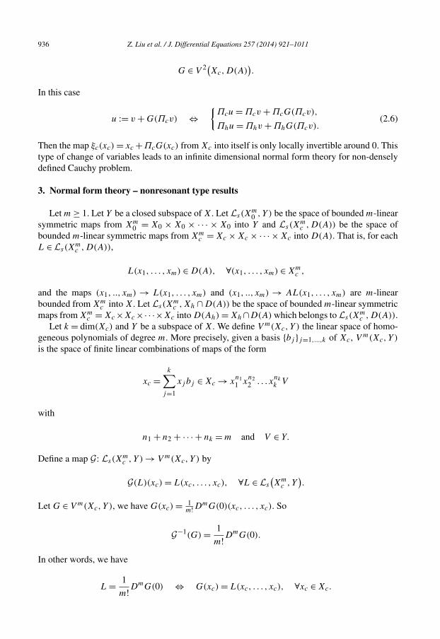
936 Z. Liu et al. / J. Differential Equations 257 (2014) 921–1011
G ∈ V 2(Xc,D(A)).
In this case
u := v + G(Πcv) ⇔{
Πcu = Πcv + ΠcG(Πcv),
Πhu = Πhv + ΠhG(Πcv).(2.6)
Then the map ξc(xc) = xc +ΠcG(xc) from Xc into itself is only locally invertible around 0. Thistype of change of variables leads to an infinite dimensional normal form theory for non-denselydefined Cauchy problem.
3. Normal form theory – nonresonant type results
Let m ≥ 1. Let Y be a closed subspace of X. Let Ls(Xm0 , Y ) be the space of bounded m-linear
symmetric maps from Xm0 = X0 × X0 × · · · × X0 into Y and Ls(X
mc ,D(A)) be the space of
bounded m-linear symmetric maps from Xmc = Xc × Xc × · · · × Xc into D(A). That is, for each
L ∈ Ls(Xmc ,D(A)),
L(x1, . . . , xm) ∈ D(A), ∀(x1, . . . , xm) ∈ Xmc ,
and the maps (x1, .., xm) → L(x1, . . . , xm) and (x1, .., xm) → AL(x1, . . . , xm) are m-linearbounded from Xm
c into X. Let Ls(Xmc ,Xh ∩ D(A)) be the space of bounded m-linear symmetric
maps from Xmc = Xc ×Xc ×· · ·×Xc into D(Ah) = Xh ∩D(A) which belongs to Ls(X
mc ,D(A)).
Let k = dim(Xc) and Y be a subspace of X. We define V m(Xc,Y ) the linear space of homo-geneous polynomials of degree m. More precisely, given a basis {bj }j=1,...,k of Xc, V m(Xc,Y )
is the space of finite linear combinations of maps of the form
xc =k∑
j=1
xj bj ∈ Xc → xn11 x
n22 . . . x
nk
k V
with
n1 + n2 + · · · + nk = m and V ∈ Y.
Define a map G: Ls(Xmc ,Y ) → V m(Xc,Y ) by
G(L)(xc) = L(xc, . . . , xc), ∀L ∈ Ls
(Xm
c ,Y).
Let G ∈ V m(Xc,Y ), we have G(xc) = 1m!D
mG(0)(xc, . . . , xc). So
G−1(G) = 1
m!DmG(0).
In other words, we have
L = 1DmG(0) ⇔ G(xc) = L(xc, . . . , xc), ∀xc ∈ Xc.
m!
Z. Liu et al. / J. Differential Equations 257 (2014) 921–1011 937
It follows that G is a bijection from Ls(Xmc ,Y ) into V m(Xc,Y ). So we can also define
V m(Xc,D(A)) as
V m(Xc,D(A)
) := G(Ls
(Xm
c ,D(A)))
.
In order to use the usual formalism in the context of normal form theory, we now define the Liebracket (Guckenheimer and Holmes [26, page 141]). Recall that
Xc = X0c ⊂ D(A0) ⊂ D(A),
so the following definition makes sense.
Definition 3.1. Let Assumptions 2.1, 2.2 and 2.4 be satisfied. Then for each G ∈ V m(Xc,D(A)),we define the Lie bracket
[A,G](xc) := DG(xc)(Axc) − AG(xc), ∀xc ∈ Xc. (3.1)
Recalling that Ac ∈ L(Xc) is the part of A in Xc, we obtain
[A,G](xc) = DG(xc)(Acxc) − AG(xc), ∀xc ∈ Xc.
Set L := 1m!D
mG(0) ∈ Ls(Xmc ,D(A) ∩ Xh). We also have
DG(xc)(y) = mL(y,xc, . . . , xc), DG(xc)Acxc = mL(Acxc, xc, . . . , xc),
and
[A,G](xc) = d
dt
[L(eActxc, . . . , eActxc
)](0) − AL(xc, . . . , xc). (3.2)
We consider two cases when G belongs to different subspaces, namely, G ∈ V m(Xc,
D(A) ∩ Xh) and G ∈ V m(Xc,D(A)), respectively.
3.1. G ∈ V m(Xc,D(A) ∩ Xh)
We consider the change of variables (2.2), i.e.,
u = v + G(Πcv).
Then
G(xc) := L(xc, xc, . . . , xc), ∀xc ∈ Xc.
The map xc → AG(xc) is differentiable and
D(AG)(xc)(y) = ADG(xc)(y) = mAL(y,xc, . . . , xc).

938 Z. Liu et al. / J. Differential Equations 257 (2014) 921–1011
Define a map ξ : X → X by
ξ(x) := x + G(Πcx), ∀x ∈ X.
Since the range of G is included in Xh, we obtain the following equivalence
y = ξ(x) ⇔ x = ξ−1(y),
where
ξ−1(y) := y − G(Πcy), ∀y ∈ X,
and
Πcξ−1(x) = Πcx, ∀x ∈ X.
Finally, since G(x) ∈ D(A), we have
ξ(D(A)
)⊂ D(A) and ξ−1(D(A))⊂ D(A).
The following result justifies the change of variables (2.2).
Lemma 3.2. Let Assumptions 2.1, 2.2 and 2.4 be satisfied. Let L ∈ Ls(Xmc ,Xh ∩D(A)). Assume
that u ∈ C([0, τ ],X) is an integrated solution of the Cauchy problem
du(t)
dt= Au(t) + F
(u(t)
), t ∈ [0, τ ], u(0) = x ∈ D(A). (3.3)
Then v(t) = ξ−1(u(t)) is an integrated solution of the system
dv(t)
dt= Av(t) + H
(v(t)
), t ∈ [0, τ ], v(0) = ξ−1(x) ∈ D(A), (3.4)
where H : D(A) → X is the map defined by
H(ξ(x)
)= F(ξ(x)
)− [A,G](Πcx) − DG(Πcx)[ΠcF
(ξ(x)
)].
Conversely, if v ∈ C([0, τ ],X) is an integrated solution of (3.4), then u(t) = ξ(v(t)) is an inte-grated solution of (3.3).
Proof. Assume that u ∈ C([0, τ ],X) is an integrated solution of the system (3.3), that is,
t∫u(l)dl ∈ D(A), ∀t ∈ [0, τ ],
0
Z. Liu et al. / J. Differential Equations 257 (2014) 921–1011 939
and
u(t) = x + A
t∫0
u(l)dl +t∫
0
F(u(l)
)dl, ∀t ∈ [0, τ ].
Set
v(t) = ξ−1(u(t)), ∀t ∈ [0, τ ].
We have
A
t∫0
v(l)dl = A
t∫0
u(l)dl −t∫
0
AG(Πcu(l)
)dl
= u(t) − x −t∫
0
F(u(l)
)dl −
t∫0
AG(Πcu(l)
)dl
= u(t) − G(Πcu(t)
)− (x − G(Πcx))
+ (G(Πcu(t))− G(Πcx)
)−
t∫0
F(u(l)
)dl −
t∫0
AG(Πcu(l)
)dl
= v(t) − ξ−1(x) + (G(Πcu(t))− G(Πcx)
)−
t∫0
F(u(l)
)dl −
t∫0
AG(Πcu(l)
)dl.
Since dim(Xc) < +∞, t → Πcu(t) satisfies the following ordinary differential equations
dΠcu(t)
dt= A0cΠcu(t) + ΠcF
(u(t)
).
By integrating both sides of the above ordinary differential equations, we obtain
G(Πcu(t)
)− G(Πcx) =t∫
0
DG(Πcu(l)
)(dΠcu(l)
dl
)dl
=t∫
0
DG(Πcu(l)
)(A0cΠcu(l)
)+ DG(Πcu(l)
)(ΠcF
(u(l)
))dl.
It follows that

940 Z. Liu et al. / J. Differential Equations 257 (2014) 921–1011
A
t∫0
v(l)dl = v(t) − ξ(x)
+t∫
0
DG(Πcu(l)
)[A0cΠcu(l) + ΠcF
(u(l)
)]dl
−t∫
0
F(u(l)
)dl −
t∫0
AG(Πcu(l)
)dl.
Thus
v(t) = ξ(x) + A
t∫0
v(l)dl +t∫
0
H(v(l)
)dl,
in which
H(ξ(x)
)= F(ξ(x)
)+ AG(Πcξ(x)
)− DG
(Πcξ(x)
)[AcΠcξ(x) + ΠcF
(ξ(x)
)].
Since Πcξ = Πc, the first implication follows. The converse follows from the first implicationby replacing F by H and ξ by ξ−1. �
Set for each η > 0,
BCη(R,X) :={f ∈ C(R,X) : sup
t∈Re−η|t |∥∥f (t)
∥∥< +∞}.
The following lemma was proved in Magal and Ruan [43, Lemma 4.6].
Lemma 3.3. Let Assumptions 2.1, 2.2 and 2.4 be satisfied. For each η ∈ (0,−ω0(A0s)), thefollowing properties are satisfied:
(i) For each f ∈ BCη(R,X) and each t ∈R,
Ks(f )(t) := limτ→−∞ Πs
(SA � f (τ + .)
)(t − τ) exists.
(ii) Ks is a bounded linear operator from BCη(R,X) into itself.(iii) For each t, s ∈ R with t ≥ s,
Ks(f )(t) = TA0s(t − s)Ks(f )(s) + Πs
(SA � f (s + .)
)(t − s).
The following lemma was proved in Magal and Ruan [43, Lemma 4.7].
Z. Liu et al. / J. Differential Equations 257 (2014) 921–1011 941
Lemma 3.4. Let Assumptions 2.1, 2.2 and 2.4 be satisfied. Let η ∈ (0, infλ∈σ(A0u) Re(λ)) be fixed.Then we have the following:
(i) For each f ∈ BCη(R,X) and each t ∈R,
Ku(f )(t) := −+∞∫0
e−A0ulΠuf (l + t)dl = −+∞∫t
e−A0u(l−t)Πuf (l)dl
exists.(ii) Ku is a bounded linear operator from BCη(R,X) into itself.
(iii) For each f ∈ BCη(R,X) and each t, s ∈R with t ≥ s,
Ku(f )(t) = eA0u(t−s)Ku(f )(s) + Π0u
(SA � f (s + .)
)(t − s).
We now prove the following lemma.
Lemma 3.5. Let Assumptions 2.1, 2.2 and 2.4 be satisfied. If
f (t) = tkeλtx
for some k ∈N, λ ∈ iR, and x ∈ X, then
(Ku + Ks)(Πhf )(0) = (−1)kk!(λI − Ah)−(k+1)Πhx ∈ D(Ah) ⊂ D(A).
Proof. We have
Ku(f )(0) = −+∞∫0
eλllke−A0ulΠuxdl
= − dk
dλk
+∞∫0
eλle−A0ulΠuxdl
= − dk
dλk(−λI + A0u)−1Πux
= dk
dλk(λI − A0u)−1Πux
= (−1)kk!(λI − A0u)−(k+1)Πux.
Similarly, we have for μ > ωA that
(μI − A)−1Ks(f )(0) = lim (μI − A)−1Πs
(SA � f (τ + .)
)(−τ)
τ→−∞
942 Z. Liu et al. / J. Differential Equations 257 (2014) 921–1011
= limτ→−∞
−τ∫0
TA0s(−τ − s)(μI − A)−1Πsf (s + τ)ds
= limr→+∞
r∫0
TA0s(r − s)(μI − A)−1Πsf (s − r)ds
=+∞∫0
TA0s(l)(μI − A)−1Πsf (−l)dl.
So we obtain that
(μI − A)−1Ks(f )(0) =+∞∫0
(−l)ke−λlTA0(l)(μI − A)−1Πsxdl
= dk
dλk(λI − A0)−1(μI − A)−1Πsx
= (−1)kk!(λI − A0)−(k+1)(μI − A)−1Πsx
= (μI − A)−1(−1)kk!(λI − As)−(k+1)Πsx.
Since (μI − A)−1 is one-to-one, we deduce that
Ks(f )(t) = (−1)kk!(λI − As)−(k+1)Πsx
and the result follows. �The first result of this section is the following proposition which is related to nonresonant
normal forms for ordinary differential equations (see Guckenheimer and Holmes [26], Chow andHale [8], and Chow et al. [9]).
Proposition 3.6. Let Assumptions 2.1, 2.2 and 2.4 be satisfied. For each R ∈ V m(Xc,Xh), thereexists a unique map G ∈ V m(Xc,Xh ∩ D(A)) such that
[A,G](xc) = R(xc), ∀xc ∈ Xc. (3.5)
Moreover, (3.5) is equivalent to
G(xc) = (Ku + Ks)(R(eAc.xc
))(0),
or
L(x1, . . . , xm) = (Ku + Ks)(H(eAc.x1, . . . , eAc.xm
))(0),
with L := 1 DmG(0) and H := 1 DmR(0).
m! m!
Z. Liu et al. / J. Differential Equations 257 (2014) 921–1011 943
Proof. Assume first that G ∈ V m(Xc,Xh ∩ D(A)) satisfies (3.5). Then L = 1m!D
mG(0) ∈Ls(X
mc ,Xh ∩ D(A)) satisfies
d
dt
[L(eActx1, . . . , eAct xm
)](0) = AhL(x1, . . . , xm) + H(x1, . . . , xm),
where H = 1m!D
mR(0) ∈ Ls(Xmc ,Xh). Then (3.5) is satisfied if and only if for each
(x1, . . . , xm) ∈ Xmc and each t ∈R,
d
dt
[L(eActx1, . . . , eActxm
)](t) = AhL
(eActx1, . . . , eAct xm
)+ H
(eActx1, . . . , eAct xm
). (3.6)
Set
v(t) := L(eActx1, . . . , eActxm
), ∀t ∈R,
and
w(t) := H(eActx1, . . . , eAct xm
), ∀t ∈R.
The Cauchy problem (3.6) can be rewritten as
dv(t)
dt= Ahv(t) + w(t), ∀t ∈R. (3.7)
Since L and H are bounded multilinear maps and σ(A0c) ⊂ iR, it follows that for each η > 0,
v ∈ BCη(R,X) and w ∈ BCη(R,X).
Let η ∈ (0, min(−ω0(A0s), infλ∈σ(A0u) Re(λ))). By projecting (3.7) on Xu, we have
dΠuv(t)
dt= AuΠuv(t) + Πuw(t),
or equivalently, ∀t, s ∈ R with t ≥ s,
Πuv(t) = eAu(t−s)Πuv(s) +t∫
s
eAu(t−l)Πuw(l)dl,
Πuv(s) = e−Au(t−s)Πuv(t) −t∫
s
e−Au(l−s)Πuw(l)dl.
By using the fact that v ∈ BCη(R,X), we obtain when t goes to +∞ that
Πuv(s) = Ku(Πuw)(s), ∀s ∈R.

944 Z. Liu et al. / J. Differential Equations 257 (2014) 921–1011
Thus, for s = 0 we have
ΠuL(x1, . . . , xm) = Ku
(ΠuH
(eAc.x1, . . . , eAc.xm
))(0). (3.8)
By projecting (3.7) on Xs , we obtain
dΠsv(t)
dt= AsΠsv(t) + Πsw(t),
or equivalently, ∀t, s ∈R with t ≥ s,
Πsv(t) = TAs (t − s)Πsv(s) + (SAs � Πsw(. + s))(t − s).
By using the fact that v ∈ BCη(R,X), we have when s goes to −∞ that
Πsv(t) = Ks(Πsw)(t), ∀t ∈R.
Thus, for t = 0 it follows that
ΠsL(x1, . . . , xm) = Ks
(ΠsH
(eAc.x1, . . . , eAc.xm
))(0). (3.9)
Summing up (3.8) and (3.9), we deduce that
L(x1, . . . , xm) = (Ku + Ks)(H(eAc.x1, . . . , eAc.xm
))(0). (3.10)
Conversely, assume that L(x1, . . . , xm) is defined by (3.10) and set
v(t) := (Ku + Ks)(H(eAc(t+.)x1, . . . , eAc(t+.)xm
))(0), ∀t ∈R.
Then we have
v(t) = L(eActx1, . . . , eActxm
), ∀t ∈ R.
Moreover, using Lemma 3.3(iii) and Lemma 3.4(iii), we deduce that for each t, s ∈R with t ≥ s,
v(t) = TA0(t − s)v(s) + (SA � w(. + s))(t − s),
or equivalently,
v(t) = v(s) + A
t∫s
v(l)dl +t∫
s
w(l)dl.
Since t → v(t) is continuously differentiable and A is closed, we deduce that
v(t) ∈ D(A), ∀t ∈ R,
Z. Liu et al. / J. Differential Equations 257 (2014) 921–1011 945
and
dv(t)
dt= Av(t) + w(t), ∀t ∈R.
The result follows. �Remark 3.7 (An explicit formula for L). Since n := dim(Xc) < +∞, we can find a basis{e1, . . . , en} of Xc such that the matrix of Ac (with respect to this basis) is reduced to the Jordanform. Then for each xc ∈ Xc, eActxc is a linear combination of elements of the form
tkeλtxj
for some k ∈ {1, . . . , n}, some λ ∈ σ(Ac) ⊂ iR, and some xj ∈ {e1, . . . , en}. Let λ1, . . . , λm ∈σ(Ac) ⊂ iR, x1, . . . , xm ∈ {e1, . . . , en}, k1, . . . , km ∈ {1, . . . , n}. Define
f (t) := H(tk1eλ1t.x1, . . . , tkmeλmt.xm
), ∀t ∈R.
Since H is m-linear, we obtain
f (t) = tkeλy
with
k = k1 + k2 + · · · + km, λ = λ1 + · · · + λm,
and
y = H(x1, . . . , xm).
Now by using Lemma 3.5, we obtain the explicit formula
(Ku + Ks)(H((.)k1eλ1.x1, . . . , (.)kmeλm.xm
))(0) = (−1)kk!(λI − Ah)−(k+1)Πhy ∈ D(A).
3.2. G ∈ V m(Xc,D(A))
From (3.2), for each H ∈ V m(Xc,X), to find G ∈ V m(Xc,D(A)) satisfying
[A,G] = H, (3.11)
is equivalent to finding L ∈ Ls(Xmc ,D(A)) satisfying
d
dt
[L(eActx1, . . . , eAct xm
)]t=0 = AL(x1, . . . , xm) + H (x1, . . . , xm) (3.12)
for each (x1, . . . , xm) ∈ Xmc with
G(H ) = H.
946 Z. Liu et al. / J. Differential Equations 257 (2014) 921–1011
Define Θcm : V m(Xc,Xc) → V m(Xc,Xc) by
Θcm(Gc) := [Ac,Gc], ∀Gc ∈ V m(Xc,Xc), (3.13)
and Θhm : V m(Xc,Xh ∩ D(A)) → V m(Xc,Xh) by
Θhm(Gh) := [A,Gh], ∀Gh ∈ V m
(Xc,Xh ∩ D(A)
).
We decompose V m(Xc,Xc) into the direct sum
V m(Xc,Xc) =Rcm ⊕ Cc
m, (3.14)
where
Rcm := R
(Θc
m
)is the range of Θc
m, and Ccm is some complementary space of Rc
m into V m(Xc,Xc).The range of the linear operator Θc
m can be characterized by using the so-called non-resonancetheorem. The second result of this section is the following theorem.
Proposition 3.8. Let Assumptions 2.1, 2.2 and 2.4 be satisfied. Let H ∈ Rcm ⊕V m(Xc,Xh). Then
there exists G ∈ V m(Xc,D(A)) (non-unique in general) satisfying
[A,G] = H. (3.15)
Furthermore, if N(Θcm) = {0} (the null space of Θc
m), then G is uniquely determined.
Proof. By projecting on Xc and Xh and using the fact that Xc ⊂ D(A), it follows that solvingsystem (3.11) is equivalent to finding Gc ∈ V m(Xc,Xc) and Gh ∈ V m(Xc,Xh ∩ D(A)) satisfy-ing
[Ac,Gc] = ΠcH (3.16)
and
[A,Gh] = ΠhH. (3.17)
Now it is clear that we can solve (3.16). Moreover, by using the equivalence between (3.11)and (3.12), we can apply Proposition 3.6 and deduce that (3.17) can be solved. �Remark 3.9. In practice, we often have
N(Θc
m
)∩ R(Θc
m
)= {0}.In this case, a natural splitting of V m(Xc,Xc) will be
V m(Xc,Xc) = R(Θc
m
)⊕ N(Θc
m
).
Z. Liu et al. / J. Differential Equations 257 (2014) 921–1011 947
Define Pm : V m(Xc,X) → V m(Xc,X) the bounded linear projector satisfying
Pm
(V m(Xc,X)
)=Rcm ⊕ V m(Xc,Xh), and (I −Pm)
(V m(Xc,X)
)= Ccm.
Again consider the Cauchy problem (3.3). Assume that DF(0) = 0. Without loss of generalitywe also assume that for some m ∈ {2, . . . , k},
ΠhDj F(0)|Xc×Xc×···×Xc = 0, G(ΠcD
j F(0)|Xc×Xc×···×Xc
) ∈ Ccj , (Cm−1)
for each j = 1, . . . ,m − 1.Consider the change of variables
u(t) = w(t) + G(Πcw(t)
)(3.18)
and the map I + 1m!G ◦ Πc : D(A) → D(A) is locally invertible around 0. We will show that
we can find G ∈ V m(Xc,D(A)) such that after the change of variables (3.18) we can rewrite thesystem (3.3) as
dw(t)
dt= Aw(t) + H
(w(t)
), for t ≥ 0, and w(0) = (I + G ◦ Πc)x ∈ D(A), (3.19)
where H satisfies the condition (Cm). This will provide a normal form method which is analo-gous to the one proposed by Faria and Magalhães [24].
Lemma 3.10. Let Assumptions 2.1, 2.2 and 2.4 be satisfied. Let G ∈ V m(Xc,D(A)). Assumethat u ∈ C([0, τ ],X) is an integrated solution of the Cauchy problem (3.3). Then w(t) = (I +G ◦ Πc)
−1(u(t)) is an integrated solution of the system (3.19), where H : D(A) → X is the mapdefined by
H(w(t)
)= F(w(t)
)− [A,G](Πcw(t))+ O
(∥∥w(t)∥∥m+1)
.
Conversely, if w ∈ C([0, τ ],X) is an integrated solution of (3.19), then u(t) = (I + G ◦ Πc)w(t)
is an integrated solution of (3.3).
Lemma 3.10 can be proved similarly as Lemma 3.2, here we omit it.
Proposition 3.11. Let Assumptions 2.1, 2.2 and 2.4 be satisfied. Let r > 0 and letF : BX0(0, r) → X be a map. Assume that there exists an integer k ≥ 1 such that F is k-timecontinuously differentiable in BX0(0, r) with F(0) = 0 and DF(0) = 0. Let m ∈ {2, . . . , k} besuch that F satisfies the condition (Cm−1). Then there exists a map G ∈ V m(Xc,D(A)) suchthat after the change of variables
u(t) = w(t) + G(Πcw(t)
),
we can rewrite system (3.3) as (3.19) and H satisfies the condition (Cm), where
H(w(t)
)= F(w(t)
)− [A,G](Πcw(t))+ O
(∥∥w(t)∥∥m+1)
.
948 Z. Liu et al. / J. Differential Equations 257 (2014) 921–1011
Proof. Let xc ∈ Xc. We have
H(xc) = F(xc) − [A,G](Πcxc) + O(‖xc‖m+1).
It follows that
H(xc) = 1
2!D2F(0)(xc, xc) + · · · + 1
(m − 1)!Dm−1F(0)(xc, . . . , xc)
+Pm
[1
m!DmF(0)(xc, . . . , xc)
]+ (I −Pm)
[1
m!DmF(0)(xc, . . . , xc)
]− [A,G](xc) + O
(‖xc‖m+1)since DF(0) = 0. Moreover, by using Proposition 3.8 we obtain that there exists a map G ∈V m(Xc,D(A)) such that
[A,G](xc) =Pm
[1
m!DmF(0)(xc, . . . , xc)
].
Hence,
H(xc) = 1
2!D2F(0)(xc, xc) + · · · + 1
(m − 1)!Dm−1F(0)(xc, . . . , xc)
+ (I −Pm)
[1
m!DmF(0)(xc, . . . , xc)
]+ O
(‖xc‖m+1). (3.20)
By the assumption, we have for all j = 1, . . . ,m − 1 that
ΠhDj H(0)|Xc×Xc×···×Xc = ΠhDj F(0)|Xc×Xc×···×Xc = 0
and
G(ΠcD
j H(0)|Xc×Xc×···×Xc
)= G(ΠcD
j F(0)|Xc×Xc×···×Xc
) ∈ Ccj .
Now by using (3.20), we have
1
m!ΠhDmH(0)|Xc×Xc×···×Xc = ΠhG−1[(I −Pm)
(1
m!DmF(0)(xc, . . . , xc)
)]= 0
and
G(ΠcD
mH(0)|Xc×Xc×···×Xc
)= G{ΠcG−1[(I −Pm)
(DmF(0)(xc, . . . , xc)
)]} ∈ Ccm.
The result follows. �

Z. Liu et al. / J. Differential Equations 257 (2014) 921–1011 949
4. Normal form computation
In this section we provide the method to compute the Taylor expansion at any order andnormal form of the reduced system of a system topologically equivalent to the original system:⎧⎨⎩
du(t)
dt= Au(t) + F
(u(t)
), t ≥ 0,
u(0) = x ∈ D(A).
(4.1)
Assumption 4.1. Assume that F ∈ Ck(D(A),X) for some integer k ≥ 2 with
F(0) = 0 and DF(0) = 0.
Set
F1 := F.
Once again we consider two cases, namely, G ∈ V m(Xc,D(A) ∩ Xh) and G ∈ V m(Xc,D(A)),respectively.
4.1. G ∈ V m(Xc,D(A) ∩ Xh)
For j = 2, . . . , k, we apply Proposition 3.6. Then there exists a unique function Gj ∈V j (Xc,Xh ∩ D(A)) satisfying
[A,Gj ](xc) = 1
j !ΠhDj Fj−1(0)(xc, . . . , xc), ∀xc ∈ Xc. (4.2)
Define ξj : X → X and ξ−1j : X → X by
ξj (x) := x + Gj (Πcx) and ξ−1j (x) := x − Gj (Πcx), ∀x ∈ X.
Then
Fj (x) := Fj−1(ξj (x)
)− [A,Gj ](Πcx) − DGj (Πcx)[ΠcFj−1
(ξj (x)
)].
Moreover, we have for x ∈ X0 that
ΠcFj (x) = ΠcFj−1(ξj (x)
)= ΠcFj−1(x + Gj (Πcx)
).
Since the range of Gj is included in Xh, by induction we have
ΠcFj (x) = ΠcF(x + G2(Πcx) + G3(Πcx) + · · · + Gj (Πcx)
).
Now, we obtain
ΠhDj Fk(0)|Xc×Xc×···×Xc = 0 for all j = 1, . . . , k.

950 Z. Liu et al. / J. Differential Equations 257 (2014) 921–1011
Setting
uk(t) = ξ−1k ◦ ξ−1
k−1 ◦ · · · ◦ ξ−12
(u(t)
)= u(t) − G2
(Πcu(t)
)− G3(Πcu(t)
)− · · · − Gk
(Πcu(t)
),
we deduce that uk(t) is an integrated solution of the system⎧⎨⎩duk(t)
dt= Auk(t) + Fk
(uk(t)
), t ≥ 0,
uk(0) = xk ∈ D(A).
(4.3)
Applying Theorem 2.7 and Lemma 2.8 to system (4.3), we obtain the following result which isone of the main results of this paper.
Theorem 4.2. Let Assumptions 2.1, 2.2, 2.4, and 4.1 be satisfied. Then by using the change ofvariables ⎧⎪⎨⎪⎩
uk(t) = u(t) − G2(Πcu(t)
)− G3(Πcu(t)
)− · · · − Gk
(Πcu(t)
)⇔
u(t) = uk(t) + G2(Πcuk(t)
)+ G3(Πcuk(t)
)+ · · · + Gk
(Πcuk(t)
),
the map t → u(t) is an integrated solution of the Cauchy problem (4.1) if and only if t → uk(t)
is an integrated solution of the Cauchy problem (4.3). Moreover, the reduced system of Cauchyproblem (4.3) is given by the ordinary differential equations on Xc:
dxc(t)
dt= Acxc(t) + ΠcF
[xc(t) + G2(xc(t))
+ G3(xc(t)) + · · · + Gk(xc(t))
]+ Rc
(xc(t)
), (4.4)
where the remainder term Rc ∈ Ck(Xc,Xc) satisfies
Dj Rc(0) = 0 for each j = 1, . . . , k,
or in other words Rc(xc(t)) is a remainder term of order k.If we assume in addition that F ∈ Ck+2(D(A),X), then the map Rc ∈ Ck+2(Xc,Xc) and
Rc(xc(t)) is a remainder term of order k + 2, that is
Rc(xc) = ‖xc‖k+2O(xc), (4.5)
where O(xc) is a function of xc which remains bounded when xc goes to 0, or equivalently,
Dj Rc(0) = 0 for each j = 1, . . . , k + 1.
Proof. By Theorem 2.7 and Lemma 2.8, there exists Ψk ∈ Ck(Xc,Xh) such that the reducedsystem of (4.3) is given by
Z. Liu et al. / J. Differential Equations 257 (2014) 921–1011 951
dxc(t)
dt= Acxc(t) + ΠcF
[xc(t) + G2
(xc(t)
)+ G3(xc(t)
)+ · · · + Gk
(xc(t)
)+ Ψk
(xc(t)
)]and
Dj Ψk(0) = 0 for j = 1, . . . , k.
By setting
Rc(xc) = ΠcF[xc + G2(xc) + G3(xc) + · · · + Gk(xc) + Ψk(xc)
]− ΠcF
[xc + G2(xc) + G3(xc) + · · · + Gk(xc)
],
we obtain the first part of the theorem. If we assume in addition that F ∈ Ck+2(D(A),X), thenΨk ∈ Ck+2(Xc,Xh). Thus,
Rc ∈ Ck+2(Xc,Xc).
Set
h(xc) := xc + G2(xc) + G3(xc) + · · · + Gk(xc).
We have
Rc(xc) = Πc
{F[h(xc) + Ψk(xc)
]− F[h(xc)
]}= Πc
1∫0
DF(h(xc) + sΨk(xc)
)(Ψk(xc)
)ds.
Define
h(xc) := h(xc) + sΨk(xc).
Since DF(0) = 0, we have
DF(h(xc)
)(Ψk(xc)
)= DF(0)(Ψk(xc)
)+ 1∫0
D2F(lh(xc)
)(h(xc),Ψk(xc)
)dl
=1∫
0
D2F(lh(xc)
)(h(xc),Ψk(xc)
)dl.
Hence,
Rc(xc) = Πc
1∫ 1∫D2F
(l(h(xc) + sΨk(xc)
))(h(xc) + sΨk(xc),Ψk(xc)
)dlds
0 0
952 Z. Liu et al. / J. Differential Equations 257 (2014) 921–1011
and h(xc) is a term of order 1, Ψk(xc) is a term of order k + 1, it follows that (4.5) holds. Thiscompletes the proof. �Remark 4.3. In order to apply the above approach, we first need to compute Πc and Ac, thenΠh := I − Πc can be derived. The point to apply the above procedure is to solve system (4.2).To do this, one may compute
(λI − Ah)−k 1
j !ΠhDj F(0) (4.6)
for each λ ∈ iR and each k ≥ 1 by using Remark 3.7, or one may directly solve system (4.2) bycomputing Πh
1j !D
j Fj−1. This last approach will involve the computation of (4.6) for some spe-cific values of λ ∈ iR and some specific values of k ≥ 1. This turns out to be the main difficultyin applying the above method.
In Section 5, we will use the last part of Theorem 4.2 to avoid some unnecessary computations.We will apply this theorem for k = 2, F in C4, and the remainder term Rc(xc) of order 4. Thismeans that if we want to compute the Taylor expansion of the reduced system to the order 3(which is very common in such a context), we only need to compute G2. So in application thelast part of Theorem 4.2 will help to avoid a lot of computations.
4.2. G ∈ V m(Xc,D(A))
Now we apply Proposition 3.11 recursively to (4.1). Set
u1 := u.
For m = 2, . . . , k, let Gm ∈ V m(Xc,D(A)) be defined such that
[A,Gm](xc) =Pm
[1
m!DmFm−1(0)(xc, . . . , xc)
]for each xc ∈ Xc.
We use the change of variables
um−1 = um + Gm(Πcum).
Then we consider Fm given by Proposition 3.11 and satisfying
Fm(um) = Fm−1(um) − [A,Gm](Πcum) + O(‖um‖m+1).
By applying Proposition 3.11, we have
ΠhDj Fm(0)|Xc×Xc×···×Xc = 0, for all j = 1, . . . ,m,
and
G(ΠcD
j Fm(0)|Xc×Xc×···×Xc
) ∈ Cc, for all j = 1, . . . ,m.
j
Z. Liu et al. / J. Differential Equations 257 (2014) 921–1011 953
Thus by using the change of variables locally around 0
uk(t) = (I + GkΠc)−1 . . . (I + G3Πc)
−1(I + G2Πc)−1u(t),
we deduce that uk(t) is an integrated solution of system (4.3). Applying Theorem 2.7 andLemma 2.8 to the above system, we obtain the following result which is the main result of thispaper and indicates that systems (4.1) and (4.3) are locally topologically equivalent around 0.
Theorem 4.4. Let Assumptions 2.1, 2.2, 2.4, and 4.1 be satisfied. Then by using the change ofvariables locally around 0⎧⎪⎨⎪⎩
uk(t) = (I + GkΠc)−1 . . . (I + G3Πc)
−1(I + G2Πc)−1u(t)
⇔u(t) = (I + G2Πc)(I + G3Πc) . . . (I + GkΠc)uk(t),
the map t → u(t) is an integrated solution of the Cauchy problem (4.1) if and only if t → uk(t)
is an integrated solution of the Cauchy problem (4.3). Moreover, the reduced equation of Cauchyproblem (4.3) is given by the ordinary differential equations on Xc:
dxc(t)
dt= Acxc(t) +
k∑m=2
1
m!ΠcDmFk(0)
(xc(t), . . . , xc(t)
)+ Rc
(xc(t)
),
where
G(
1
m!ΠcDmFk(0)|Xc×Xc×···×Xc
)∈ Cc
m, for all m = 1, . . . , k,
and the remainder term Rc ∈ Ck(Xc,Xc) satisfies
Dj Rc(0) = 0 for each j = 1, . . . , k,
or in other words Rc(xc(t)) is a remainder term of order k. If we assume in addition that F ∈Ck+2(D(A),X). Then the reduced equation of Cauchy problem (4.3) is given by the ordinarydifferential equations on Xc:
dxc(t)
dt= Acxc(t) +
k+1∑m=2
1
m!ΠcDmFk(0)
(xc(t), . . . , xc(t)
)+ Rc
(xc(t)
),
the map Rc ∈ Ck+2(Xc,Xc), and Rc(xc(t)) is a remainder term of order k + 2, that is
Rc(xc) = ‖xc‖k+2O(xc),
where O(xc) is a function of xc which remains bounded when xc goes to 0, or equivalently,
Dj Rc(0) = 0 for each j = 1, . . . , k + 1.

954 Z. Liu et al. / J. Differential Equations 257 (2014) 921–1011
Proof. By Theorem 2.7 and Lemma 2.8, there exists Ψk ∈ Ck(Xc,Xh) such that the reducedsystem of (4.3) is given by
dxc(t)
dt= Acxc(t) + ΠcFk
[xc(t) + Ψk
(xc(t)
)]and
Dj Ψk(0) = 0 for j = 1, . . . , k.
By setting
Rc(xc) = ΠcFk
[xc + Ψk(xc)
]− ΠcFk(xc),
we obtain the first part of the theorem. If we assume in addition that F ∈ Ck+2(D(A),X), thenΨk ∈ Ck+2(Xc,Xh). Thus, Rc ∈ Ck+2(Xc,Xc) and
Rc(xc) = Πc
{Fk
[xc + Ψk(xc)
]− Fk(xc)}
= Πc
1∫0
DFk
(xc + sΨk(xc)
)(Ψk(xc)
)ds.
Set
h(xc) := xc + sΨk(xc).
Since DF(0) = 0, we have
DFk
(h(xc)
)(Ψk(xc)
)= DFk(0)(Ψk(xc)
)+ 1∫0
D2Fk
(lh(xc)
)(h(xc),Ψk(xc)
)dl
=1∫
0
D2Fk
(lh(xc)
)(h(xc),Ψk(xc)
)dl.
Hence,
Rc(xc) = Πc
1∫0
1∫0
D2Fk
(l(xc + sΨk(xc)
))(xc + sΨk(xc),Ψk(xc)
)dlds
and Ψk(xc) is a term of order k + 1, it follows that
Rc(xc) = ‖xc‖k+2O(xc).
The result follows. �
Z. Liu et al. / J. Differential Equations 257 (2014) 921–1011 955
5. Applications
In this section we apply the normal form theory developed in the previous sections to the twoexamples of structured models (1.2) and (1.6) introduced in Section 1. Namely, we will computethe Taylor expansion of the reduced system of model (1.2) on the center manifold and the normalform of model (1.6) on the center manifold, respectively, from which we will be able to determinethe direction of the Hopf bifurcation and stability of the bifurcating periodic solutions in thesetwo models.
5.1. A structured model of influenza A drift
We first recall the results in Magal and Ruan [44] on the existence of Hopf bifurcation in thestructured evolutionary epidemiological model (1.2) of influenza A drift. The following theoremwas proven in Magal and Ruan [44].
Proposition 5.1.
(i) Consider the curves defined by
δν = ν + 1 + ν
ν
( νc)2
1 −√
1 − 1c2
in the (ν, δ)-plane for some c ≥ 1. Then for each n ≥ 0,
νn = c
(arcsin
(−1
c
)+ 2(n + 1)π
)is a Hopf bifurcation point for system (1.5) around the branch of equilibrium points sν , where
sν(a) ={
ν(1 − Sν)e−δν(1−Sν)(a−1), if a ≥ 1,
ν(1 − Sν), if a ∈ [0, 1],
Sν =+∞∫0
sν(l)dl = 1 + δ−1ν
1 + ν−1< 1.
Moreover, the period of the bifurcating periodic orbits is close to
ωn = c arcsin
(−1
c
)+ π + 2nπ.
(ii) Consider the curves defined by
δν = ν + 1 + ν
ν
( νc)2
1 +√
1 − 12
c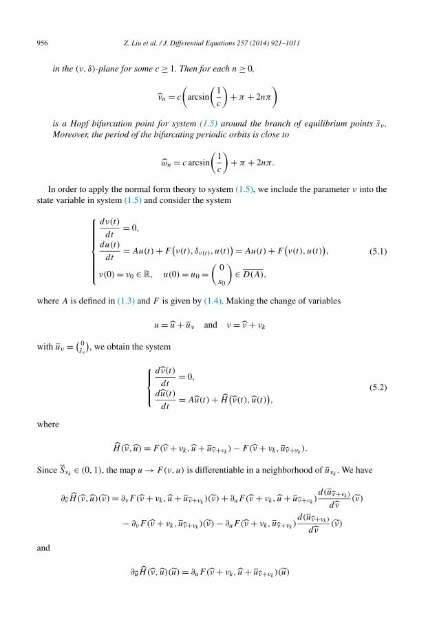
956 Z. Liu et al. / J. Differential Equations 257 (2014) 921–1011
in the (ν, δ)-plane for some c ≥ 1. Then for each n ≥ 0,
νn = c
(arcsin
(1
c
)+ π + 2nπ
)is a Hopf bifurcation point for system (1.5) around the branch of equilibrium points sν .Moreover, the period of the bifurcating periodic orbits is close to
ωn = c arcsin
(1
c
)+ π + 2nπ.
In order to apply the normal form theory to system (1.5), we include the parameter ν into thestate variable in system (1.5) and consider the system⎧⎪⎪⎪⎪⎪⎪⎨⎪⎪⎪⎪⎪⎪⎩
dν(t)
dt= 0,
du(t)
dt= Au(t) + F
(ν(t), δν(t), u(t)
)= Au(t) + F(ν(t), u(t)
),
ν(0) = ν0 ∈R, u(0) = u0 =(
0
s0
)∈ D(A),
(5.1)
where A is defined in (1.3) and F is given by (1.4). Making the change of variables
u = u + uν and ν = ν + νk
with uν = ( 0sν
), we obtain the system
⎧⎪⎨⎪⎩dν(t)
dt= 0,
du(t)
dt= Au(t) + H
(ν(t), u(t)
),
(5.2)
where
H (ν, u) = F (ν + νk, u + uν+νk) − F (ν + νk, uν+νk
).
Since Sνk∈ (0, 1), the map u → F(ν,u) is differentiable in a neighborhood of uνk
. We have
∂νH (ν, u)(ν) = ∂νF (ν + νk, u + uν+νk)(ν) + ∂uF (ν + νk, u + uν+νk
)d(uν+νk)
dν(ν)
− ∂νF (ν + νk, uν+νk)(ν) − ∂uF (ν + νk, uν+νk
)d(uν+νk)
dν(ν)
and
∂uH (ν, u)(u) = ∂uF (ν + νk, u + uν+ν )(u)
k
Z. Liu et al. / J. Differential Equations 257 (2014) 921–1011 957
with
∂uF (ν,u)(u) =( −ν
∫ +∞0 ϕ(l)dl
−δνχ[ϕ(1 − ∫ +∞0 ϕ(l)dl) − ϕ
∫ +∞0 ϕ(l)dl]
),
here u =(
0
ϕ
), u =
(0
ϕ
)∈ D(A). Hence, ∂νH (0, 0)(ν) = 0 and ∂uH (0, 0)(u) = ∂uF (νk, uνk
)(u).
Set
Y =R× X, Y0 = R× D(A)
and
Aν := A + ∂uF (ν,uν).
The following lemma is obtained in Magal and Ruan [42].
Lemma 5.2. The linear operator Aν : D(A) ⊂ X → X is a Hille–Yosida operator and
ω0,ess((Aν)0
)≤ −δν(1 − Sν) < 0.
Consider the linear operator L : D(L) ⊂ Y→Y defined by
L
(ν
u
)=(
0
(A + ∂uF (νk, uνk))u
)=(
0
Aνku
)with D(L) =R× D(A) and the map H : D(L) → Y defined by
H
(ν
u
)=( 0
W(
ν
u
)),
where W : D(L) → X is defined by
W = F (ν + νk, u + uν+νk) − F (ν + νk, uν+νk
) − ∂uF (νk, uνk)u.
Then we have
H
(0
0
)= 0 and DH
(0
0
)= 0.
Now we can reformulate system (4.2) as the following system
dw(t)
dt= Lw(t) + H
(w(t)
), w(0) = w0 ∈ D(L). (5.3)
The following lemma is a consequence of the results proved in Liu et al. [35, Section 3.1].
958 Z. Liu et al. / J. Differential Equations 257 (2014) 921–1011
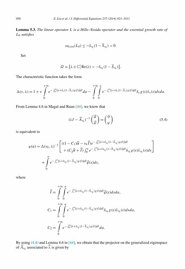
Lemma 5.3. The linear operator L is a Hille–Yosida operator and the essential growth rate ofL0 satisfies
ω0,ess(L0) ≤ −δνk(1 − Sνk
) < 0.
Set
Ω = {λ ∈ C∣∣Re(λ) > −δνk
(1 − Sνk)}.
The characteristic function takes the form
�(ν,λ) = 1 + ν
+∞∫0
e− ∫ a0 [λ+δν(1−Sν)χ(l)]dlda −
+∞∫0
a∫0
e− ∫ as [λ+δν(1−Sν)χ(l)]dlδνχ(s)sν(s)dsda.
From Lemma 4.6 in Magal and Ruan [44], we know that
(λI − Aνk)−1
(α
ϕ
)=(
0
ϕ
)(5.4)
is equivalent to
ϕ(a) = �(νk,λ)−1
[((1 − C1)α − νkI )e− ∫ a
0 [λ+δνk(1−Sνk
)χ(l)]dl
+ (C2α + I )∫ a
0 e− ∫ as [λ+δνk
(1−Sνk)χ(l)]dlδνk
χ(s)sνk(s)ds
]
+a∫
0
e− ∫ as [λ+δνk
(1−Sνk)χ(l)]dlϕ(s)ds,
where
I =+∞∫0
a∫0
e− ∫ as [λ+δνk
(1−Sνk)χ(l)]dl ϕ(s)dsda,
C1 =+∞∫0
a∫0
e− ∫ as [λ+δνk
(1−Sνk)χ(l)]dlδνk
χ(s)sνk(s)dsda,
C2 =+∞∫0
e− ∫ a0 [λ+δνk
(1−Sνk)χ(l)]dlda.
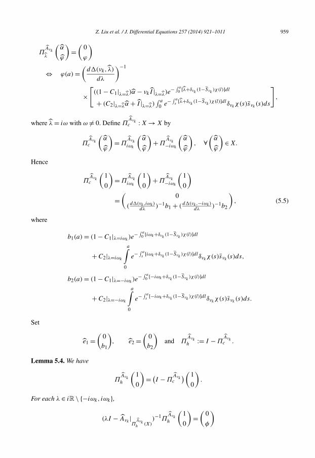
By using (4.4) and Lemma 4.6 in [44], we obtain that the projector on the generalized eigenspaceof Aν associated to λ is given by
k
Z. Liu et al. / J. Differential Equations 257 (2014) 921–1011 959
ΠAνk
λ
(α
ϕ
)=(
0
ϕ
)⇔ ϕ(a) =
(d�(νk, λ)
dλ
)−1
×[
((1 − C1|λ=λ)α − νkI |λ=λ)e− ∫ a0 [λ+δνk
(1−Sνk)χ(l)]dl
+ (C2|λ=λα + I |λ=λ)∫ a
0 e− ∫ as [λ+δνk
(1−Sνk)χ(l)]dlδνk
χ(s)sνk(s)ds
],
where λ = iω with ω �= 0. Define ΠAνkc : X → X by
ΠAνkc
(α
ϕ
)= Π
Aνk
iωk
(α
ϕ
)+ Π
Aνk−iωk
(α
ϕ
), ∀
(α
ϕ
)∈ X.
Hence
ΠAνkc
(1
0
)= Π
Aνk
iωk
(1
0
)+ Π
Aνk−iωk
(1
0
)=(
0
(d�(νk,iωk)
dλ)−1b1 + (
d�(νk,−iωk)dλ
)−1b2
), (5.5)
where
b1(a) = (1 − C1|λ=iωk)e− ∫ a
0 [iωk+δνk(1−Sνk
)χ(l)]dl
+ C2|λ=iωk
a∫0
e− ∫ as [iωk+δνk
(1−Sνk)χ(l)]dlδνk
χ(s)sνk(s)ds,
b2(a) = (1 − C1|λ=−iωk)e− ∫ a
0 [−iωk+δνk(1−Sνk
)χ(l)]dl
+ C2|λ=−iωk
a∫0
e− ∫ as [−iωk+δνk
(1−Sνk)χ(l)]dlδνk
χ(s)sνk(s)ds.
Set
e1 =(
0
b1
), e2 =
(0
b2
)and Π
Aνk
h := I − ΠAνkc .
Lemma 5.4. We have
ΠAνk
h
(1
0
)= (I − Π
Aνkc
)(1
0
).
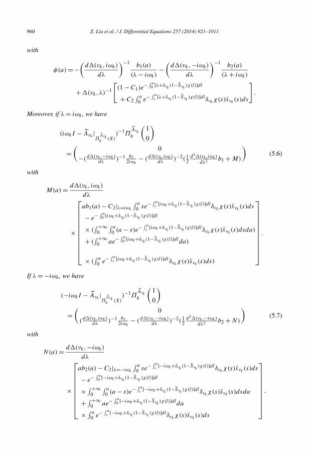
For each λ ∈ iR \ {−iωk, iωk},
(λI − Aνk| Aνk
)−1ΠAνk
h
(1)
=(
0)
Πh (X) 0 φ
960 Z. Liu et al. / J. Differential Equations 257 (2014) 921–1011
with
φ(a) = −(
d�(νk, iωk)
dλ
)−1b1(a)
(λ − iωk)−(
d�(νk,−iωk)
dλ
)−1b2(a)
(λ + iωk)
+ �(νk,λ)−1
[(1 − C1)e− ∫ a
0 [λ+δνk(1−Sνk
)χ(l)]dl
+ C2∫ a
0 e− ∫ as [λ+δνk
(1−Sνk)χ(l)]dlδνk
χ(s)sνk(s)ds
].
Moreover, if λ = iωk , we have
(iωkI − Aνk|Π
Aνkh (X)
)−1ΠAνk
h
(1
0
)=(
0
−(d�(νk,−iωk)
dλ)−1 b2
2iωk− (
d�(νk,iωk)dλ
)−2( 12
d2�(νk,iωk)
dλ2 b1 + M)
)(5.6)
with
M(a) = d�(νk, iωk)
dλ
×
⎡⎢⎢⎢⎢⎢⎢⎢⎢⎢⎢⎣
ab1(a) − C2|λ=iωk
∫ a
0 se− ∫ as [iωk+δνk
(1−Sνk)χ(l)]dlδνk
χ(s)sνk(s)ds
− e− ∫ a0 [iωk+δνk
(1−Sνk)χ(l)]dl
× (∫ +∞
0
∫ a
0 (a − s)e− ∫ as [iωk+δνk
(1−Sνk)χ(l)]dlδνk
χ(s)sνk(s)dsda)
+ (∫ +∞
0 ae− ∫ a0 [iωk+δνk
(1−Sνk)χ(l)]dlda)
× (∫ a
0 e− ∫ as [iωk+δνk
(1−Sνk)χ(l)]dlδνk
χ(s)sνk(s)ds)
⎤⎥⎥⎥⎥⎥⎥⎥⎥⎥⎥⎦.
If λ = −iωk , we have
(−iωkI − Aνk|Π
Aνkh (X)
)−1ΠAνk
h
(1
0
)=(
0
(d�(νk,iωk)
dλ)−1 b1
2iωk− (
d�(νk,−iωk)dλ
)−2( 12
d2�(νk,−iωk)
dλ2 b2 + N)
)(5.7)
with
N(a) = d�(νk,−iωk)
dλ
×
⎡⎢⎢⎢⎢⎢⎢⎢⎢⎣
ab2(a) − C2|λ=−iωk
∫ a
0 se− ∫ as [−iωk+δνk
(1−Sνk)χ(l)]dlδνk
χ(s)sνk(s)ds
− e− ∫ a0 [−iωk+δνk
(1−Sνk)χ(l)]dl
× ∫ +∞0
∫ a
0 (a − s)e− ∫ as [−iωk+δνk
(1−Sνk)χ(l)]dlδνk
χ(s)sνk(s)dsda
+ ∫ +∞0 ae− ∫ a
0 [−iωk+δνk(1−Sνk
)χ(l)]dlda
× ∫ a
0 e− ∫ as [−iωk+δνk
(1−Sνk)χ(l)]dlδνk
χ(s)sνk(s)ds
⎤⎥⎥⎥⎥⎥⎥⎥⎥⎦.

Z. Liu et al. / J. Differential Equations 257 (2014) 921–1011 961
Proof. Since
(λI − Aνk)−1
(0
b1
)= 1
(λ − iωk)
(0
b1
)and
(λI − Aνk)−1
(0
b2
)= 1
(λ + iωk)
(0
b2
),
for each λ ∈ iR \ {−iωk, iωk},
(λI − Aνk|Π
Aνkh (X)
)−1ΠAνk
h
(1
0
)= (λI − Aνk
)−1ΠAνk
h
(1
0
)=(
0
φ
).
If λ = iωk , we have
(iωkI − Aνk|Π
Aνkh (X)
)−1ΠAνk
h
(1
0
)= lim
λ→iωk
λ∈ρ(Aνk)
(λI − Aνk|Π
Aνkh (X)
)−1ΠAνk
h
(1
0
)= lim
λ→iωk
λ∈ρ(Aνk)
(0
φ
).
Note that
−(
d�(νk, iωk)
dλ
)−1b1(a)
(λ − iωk)
+ �(νk,λ)−1
[(1 − C1)e− ∫ a
0 [λ+δνk(1−Sνk
)χ(l)]dl
+ C2∫ a
0 e− ∫ as [λ+δνk
(1−Sνk)χ(l)]dlδνk
χ(s)sνk(s)ds
]
=−�(νk,λ)b1(a) + d�(νk,iωk)
dλ(λ − iωk)
[(1−C1)e
− ∫ a0 [λ+δνk
(1−Sνk)χ(l)]dl
+C2∫ a
0 e− ∫ a
s [λ+δνk(1−Sνk
)χ(l)]dlδνk
χ(s)sνk(s)ds
]d�(νk,iωk)
dλ(λ − iωk)�(νk, λ)
= (λ − iωk)2
d�(νk,iωk)dλ
(λ − iωk)�(νk, λ)
×
{−�(νk,λ)b1(a) + d�(νk,iωk)
dλ(λ − iωk)
[(1−C1)e
− ∫ a0 [λ+δνk
(1−Sνk)χ(l)]dl
+C2∫ a
0 e− ∫ a
s [λ+δνk(1−Sνk
)χ(l)]dlδνk
χ(s)sνk(s)ds
]}(λ − iωk)2
and

962 Z. Liu et al. / J. Differential Equations 257 (2014) 921–1011
limλ→iωk
(λ − iωk)2
d�(νk,iωk)dλ
(λ − iωk)�(νk, λ)= lim
λ→iωk
1d�(νk,iωk)
dλ�(νk,λ)(λ−iωk)
=(
d�(νk, iωk)
dλ
)−2
.
Therefore,
�(ν,λ) = (λ − iωk)d�(νk, iωk)
dλ+ (λ − iωk)2
2
d2�(νk, iωk)
dλ2+ (λ − iωk)
3g(λ − iωk)
with g(0) = 13!
d3�(νk,iωk)
dλ3 . Hence
limλ→iωk
{−�(νk,λ)b1(a) + d�(νk,iωk)
dλ(λ − iωk)
[(1−C1)e
− ∫ a0 [λ+δνk
(1−Sνk)χ(l)]dl
+C2∫ a
0 e− ∫ a
s [λ+δνk(1−Sνk
)χ(l)]dlδνk
χ(s)sνk(s)ds
]}(λ − iωk)2
= limλ→iωk
{−(λ − iωk)
d�(νk,iωk)dλ
[b1(a)−(1−C1)e
− ∫ a0 [λ+δνk
(1−Sνk)χ(l)]dl
−C2∫ a
0 e− ∫ a
s [λ+δνk(1−Sνk
)χ(l)]dlδνk
χ(s)sνk(s)ds
]}(λ − iωk)2
+ limλ→iωk
−((λ−iωk)2
2d2�(νk,iωk)
dλ2 )b1(a)
(λ − iωk)2
= −M(a) − 1
2
d2�(νk, iωk)
dλ2b1(a),
which implies (5.6). Similarly, if λ = −iωk , we can prove (5.7). �Lemma 5.5. We have
ΠAνk
h
(0
ψ
)= (I − Π
Aνkc
)( 0
ψ
)=(
0
ψ
)− Π
Aνkc
(0
ψ
)=(
0
ψ − ϕ1 − ϕ2
)with
ϕ1(a) =(
d�(νk, iωk)
dλ
)−1
×[
(−νkI |λ=iωk,ϕ=ψ)e− ∫ a0 [iωk+δνk
(1−Sνk)χ(l)]dl
+ I |λ=iωk,ϕ=ψ
∫ a
0 e− ∫ as [iωk+δνk
(1−Sνk)χ(l)]dlδνk
χ(s)sνk(s)ds
](5.8)
and
ϕ2(a) =(
d�(νk,−iωk))−1
dλ

Z. Liu et al. / J. Differential Equations 257 (2014) 921–1011 963
×[
(−νkI |λ=−iωk,ϕ=ψ)e− ∫ a0 [−iωk+δνk
(1−Sνk)χ(l)]dl
+ I |λ=−iωk,ϕ=ψ
∫ a
0 e− ∫ as [−iωk+δνk
(1−Sνk)χ(l)]dlδνk
χ(s)sνk(s)ds
]. (5.9)
For each λ ∈ iR \ {−iωk, iωk},
(λI − Aνk|Π
Aνkh (X)
)−1ΠAνk
h
(0
ψ
)=(
0
φ1
)with
φ1(a) = − ϕ1(a)
(λ − iωk)− ϕ2(a)
(λ + iωk)+
a∫0
e− ∫ as [λ+δνk
(1−Sνk)χ(l)]dlψ(s)ds
+ �(νk,λ)−1
[(−νkI |ϕ=ψ)e− ∫ a
0 [λ+δνk(1−Sνk
)χ(l)]dl
+ I |ϕ=ψ
∫ a
0 e− ∫ as [λ+δνk
(1−Sνk)χ(l)]dlδνk
χ(s)sνk(s)ds
].
Moreover, if λ = iωk , we have
(iωkI − Aνk|Π
Aνkh (X)
)−1ΠAνk
h
(0
ψ
)=(
0
− ϕ22iωk
+ M2 − (d�(νk,iωk)
dλ)−1(M1 + 1
2d2�(νk,iωk)
dλ2 ϕ1)
)(5.10)
with
M1(a) = aϕ1(a)d�(νk, iωk)
dλ− I |ϕ=ψ,λ=iωk
a∫0
se− ∫ as [iωk+δνk
(1−Sνk)χ(l)]dlδνk
χ(s)sνk(s)ds
− νk
( +∞∫0
a∫0
(a − s)e− ∫ as [iωk+δνk
(1−Sνk)χ(l)]dlψ(s)dsda
)e− ∫ a
0 [iωk+δνk(1−Sνk
)χ(l)]dl
+( +∞∫
0
a∫0
(a − s)e− ∫ as [iωk+δνk
(1−Sνk)χ(l)]dlψ(s)dsda
)
×( a∫
0
e− ∫ as [iωk+δνk
(1−Sνk)χ(l)]dlδνk
χ(s)sνk(s)ds
)
and
M2(a) =a∫
e− ∫ as [iωk+δνk
(1−Sνk)χ(l)]dlψ(s)ds.
0

964 Z. Liu et al. / J. Differential Equations 257 (2014) 921–1011
If λ = −iωk , we have
(−iωkI − Aνk|Π
Aνkh (X)
)−1ΠAνk
h
(0
ψ
)=(
0ϕ1
2iωk+ N2 − (
d�(νk,−iωk)dλ
)−1(N1 + 12
d2�(νk,−iωk)
dλ2 ϕ2)
)(5.11)
with
N1(a) = aϕ2(a)d�(νk,−iωk)
dλ− I |ϕ=ψ,λ=−iωk
a∫0
se− ∫ as [−iωk+δνk
(1−Sνk)χ(l)]dlδνk
χ(s)sνk(s)ds
− νk
( +∞∫0
a∫0
(a − s)e− ∫ as [−iωk+δνk
(1−Sνk)χ(l)]dlψ(s)dsda
)e− ∫ a
0 [−iωk+δνk(1−Sνk
)χ(l)]dl
+( +∞∫
0
a∫0
(a − s)e− ∫ as [−iωk+δνk
(1−Sνk)χ(l)]dlψ(s)dsda
)
×( a∫
0
e− ∫ as [−iωk+δνk
(1−Sνk)χ(l)]dlδνk
χ(s)sνk(s)ds
)
and
N2(a) =a∫
0
e− ∫ as [−iωk+δνk
(1−Sνk)χ(l)]dlψ(s)ds.
Proof. Since
(λI − Aνk|Π
Aνkh (X)
)−1(
0
ϕ1
)= 1
(λ − iωk)
(0
ϕ1
)and
(λI − Aνk|Π
Aνkh (X)
)−1(
0
ϕ2
)= 1
(λ + iωk)
(0
ϕ2
),
for each λ ∈ iR \ {−iωk, iωk},
(λI − Aνk| Aνk
)−1ΠAνk
h
(0)
=(
0)
.
Πh (X) ψ φ1
Z. Liu et al. / J. Differential Equations 257 (2014) 921–1011 965
If λ = iωk , we have
(iωkI − Aνk|Π
Aνkh (X)
)−1ΠAνk
h
(0
ψ
)= lim
λ→iωk
λ∈ρ(Aνk)
(λI − Aνk|Π
Aνkh (X)
)−1ΠAνk
h
(0
ψ
)= lim
λ→iωk
λ∈ρ(Aνk)
(0
φ1
).
Note that
− ϕ1(a)
(λ − iωk)+ �(νk,λ)−1
[(−νkI |ϕ=ψ)e− ∫ a
0 [λ+δνk(1−Sνk
)χ(l)]dl
+ I |ϕ=ψ
∫ a
0 e− ∫ as [λ+δνk
(1−Sνk)χ(l)]dlδνk
χ(s)sνk(s)ds
]
=−�(νk,λ)ϕ1(a) + (λ − iωk)
[(−νk I |ϕ=ψ )e
− ∫ a0 [λ+δνk
(1−Sνk)χ(l)]dl
+I |ϕ=ψ
∫ a0 e
− ∫ as [λ+δνk
(1−Sνk)χ(l)]dl
δνkχ(s)sνk
(s)ds
](λ − iωk)�(νk, λ)
= (λ − iωk)2
(λ − iωk)�(νk, λ)
×
{−�(νk,λ)ϕ1(a) + (λ − iωk)
[(−νk I |ϕ=ψ )e
− ∫ a0 [λ+δνk
(1−Sνk)χ(l)]dl
+I |ϕ=ψ
∫ a0 e
− ∫ as [λ+δνk
(1−Sνk)χ(l)]dl
δνkχ(s)sνk
(s)ds
]}(λ − iωk)2
and
limλ→iωk
(λ − iωk)2
(λ − iωk)�(νk, λ)=(
d�(νk, iωk)
dλ
)−1
.
We have
�(νk,λ) = (λ − iωk)d�(νk, iωk)
dλ+ (λ − iωk)2
2
d2�(νk, iωk)
dλ2+ (λ − iωk)3g(λ − iωk)
with g(0) = 13!
d3�(νk,iωk)
dλ3 . Hence
limλ→iωk
{−�(νk,λ)ϕ1(a) + (λ − iωk)
[(−νk I |ϕ=ψ )e
− ∫ a0 [λ+δνk
(1−Sνk)χ(l)]dl
+I |ϕ=ψ
∫ a0 e
− ∫ as [λ+δνk
(1−Sνk)χ(l)]dl
δνkχ(s)sνk
(s)ds
]}(λ − iωk)2
= lim
⎧⎪⎨⎪⎩−(λ − iωk)
⎡⎢⎣d�(νk,iωk)
dλϕ1(a)
−⎡⎣(−vI |ϕ=ψ )e
− ∫ a0 [λ+δνk
(1−Sνk)χ(l)]dl
+I |ϕ=ψ
∫ a0 e
− ∫ as [λ+δνk
(1−Sνk)χ(l)]dl
δνkχ(s)sνk
(s)ds
⎤⎦⎤⎥⎦⎫⎪⎬⎪⎭
2
λ→iωk (λ − iωk)
966 Z. Liu et al. / J. Differential Equations 257 (2014) 921–1011
+ limλ→iωk
−((λ−iωk)2
2d2�(νk,iωk)
dλ2 )ϕ1(a)
(λ − iωk)2
= −M1(a) − 1
2
d2�(νk, iωk)
dλ2ϕ1(a),
which yields (5.10). If λ = −iωk , we can prove (5.11) similarly. �Lemma 5.6. We have
σ(L) = σ(Aνk) ∪ {0}.
Moreover, for λ ∈ ρ(L) ∩ Ω = Ω \ (σ (Aνk) ∪ {0}), we have
(λI − L)−1(
r(�
ψ
))=( r
λ
(λI − Aνk)−1
(�
ψ
))
and the eigenvalues 0 and ±iωk of L are simple. The corresponding projectorsΠ0,Π±iωk
: Y → Y on the generalized eigenspace of L associated to 0,±iωk , respectively, aregiven by
Π0
(r
u
)=(
r
0
),
Π±iωk
(r
u
)=( 0
ΠAνk±iωk
u
).
In this context, the projectors Πc : Y → Y and Πh : Y → Y are defined by
Πc(y) = (Π0 + Πiωk+ Π−iωk
)(y), ∀y ∈ Y,
Πh(y) = (I − Πc)(y), ∀y ∈ Y.
Denote
Yc := Πc(Y ), Yh := Πh(Y ),
and
Lc := L|Yc , Lh := L|Yh.
Then we have
Πc
(0R( 1
0L1
))=(
0R
ΠAνk
iωk
( 1
0L1
)+ Π
Aνk−iωk
( 1
0L1
))=(
0R
ΠAνkc
( 1
0L1
))
and
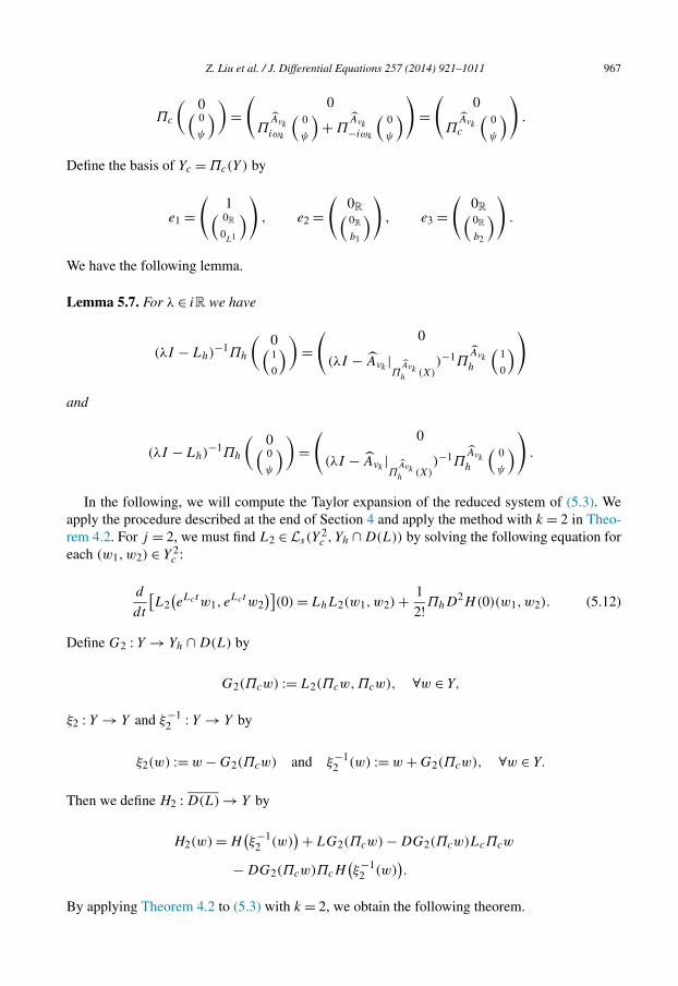
Z. Liu et al. / J. Differential Equations 257 (2014) 921–1011 967
Πc
( 0(0
ψ
))=(
0
ΠAνk
iωk
(0
ψ
)+ Π
Aνk−iωk
(0
ψ
))=(
0
ΠAνkc
(0
ψ
)) .
Define the basis of Yc = Πc(Y ) by
e1 =(
1( 0R0
L1
)) , e2 =(
0R(0Rb1
)) , e3 =(
0R(0Rb2
)) .
We have the following lemma.
Lemma 5.7. For λ ∈ iR we have
(λI − Lh)−1Πh
( 0(1
0
))=( 0
(λI − Aνk|Π
Aνkh (X)
)−1ΠAνk
h
(1
0
))
and
(λI − Lh)−1Πh
( 0(0
ψ
))=( 0
(λI − Aνk|Π
Aνkh (X)
)−1ΠAνk
h
(0
ψ
)).
In the following, we will compute the Taylor expansion of the reduced system of (5.3). Weapply the procedure described at the end of Section 4 and apply the method with k = 2 in Theo-rem 4.2. For j = 2, we must find L2 ∈ Ls(Y
2c , Yh ∩ D(L)) by solving the following equation for
each (w1,w2) ∈ Y 2c :
d
dt
[L2(eLctw1, eLctw2
)](0) = LhL2(w1,w2) + 1
2!ΠhD2H(0)(w1,w2). (5.12)
Define G2 : Y → Yh ∩ D(L) by
G2(Πcw) := L2(Πcw,Πcw), ∀w ∈ Y,
ξ2 : Y → Y and ξ−12 : Y → Y by
ξ2(w) := w − G2(Πcw) and ξ−12 (w) := w + G2(Πcw), ∀w ∈ Y.
Then we define H2 : D(L) → Y by
H2(w) = H(ξ−1
2 (w))+ LG2(Πcw) − DG2(Πcw)LcΠcw
− DG2(Πcw)ΠcH(ξ−1
2 (w)).
By applying Theorem 4.2 to (5.3) with k = 2, we obtain the following theorem.
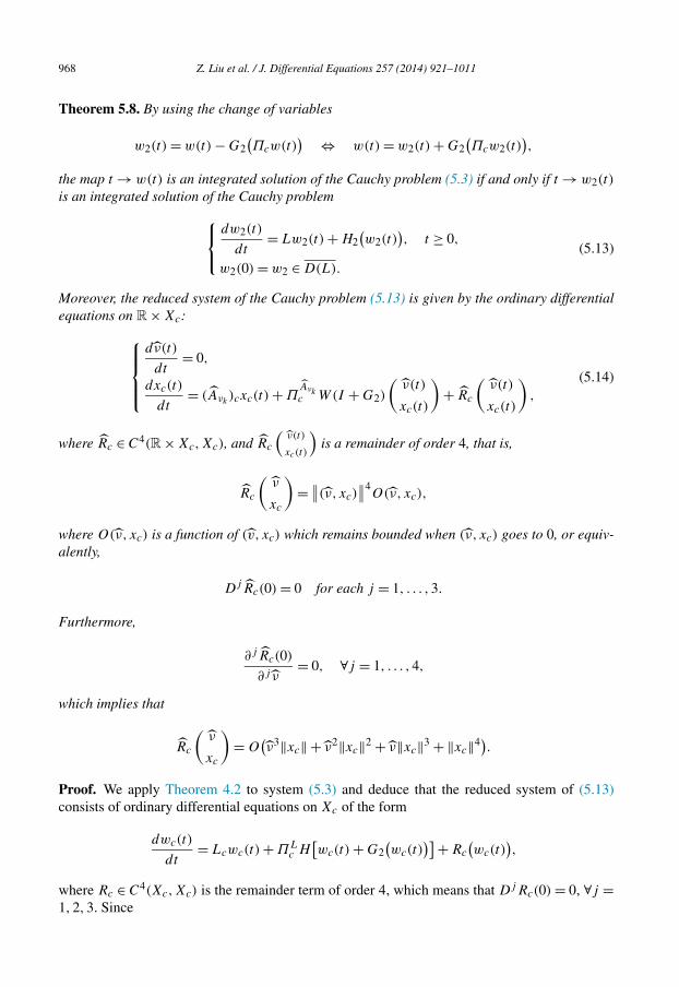
968 Z. Liu et al. / J. Differential Equations 257 (2014) 921–1011
Theorem 5.8. By using the change of variables
w2(t) = w(t) − G2(Πcw(t)
) ⇔ w(t) = w2(t) + G2(Πcw2(t)
),
the map t → w(t) is an integrated solution of the Cauchy problem (5.3) if and only if t → w2(t)
is an integrated solution of the Cauchy problem⎧⎨⎩dw2(t)
dt= Lw2(t) + H2
(w2(t)
), t ≥ 0,
w2(0) = w2 ∈ D(L).
(5.13)
Moreover, the reduced system of the Cauchy problem (5.13) is given by the ordinary differentialequations on R× Xc:⎧⎪⎪⎨⎪⎪⎩
dν(t)
dt= 0,
dxc(t)
dt= (Aνk
)cxc(t) + ΠAνkc W(I + G2)
(ν(t)
xc(t)
)+ Rc
(ν(t)
xc(t)
),
(5.14)
where Rc ∈ C4(R× Xc,Xc), and Rc
(ν(t)
xc(t)
)is a remainder of order 4, that is,
Rc
(ν
xc
)= ∥∥(ν, xc)
∥∥4O(ν, xc),
where O(ν, xc) is a function of (v, xc) which remains bounded when (ν, xc) goes to 0, or equiv-alently,
Dj Rc(0) = 0 for each j = 1, . . . , 3.
Furthermore,
∂j Rc(0)
∂j ν= 0, ∀j = 1, . . . , 4,
which implies that
Rc
(ν
xc
)= O
(ν3‖xc‖ + ν2‖xc‖2 + ν‖xc‖3 + ‖xc‖4).
Proof. We apply Theorem 4.2 to system (5.3) and deduce that the reduced system of (5.13)consists of ordinary differential equations on Xc of the form
dwc(t)
dt= Lcwc(t) + ΠL
c H[wc(t) + G2
(wc(t)
)]+ Rc
(wc(t)
),
where Rc ∈ C4(Xc,Xc) is the remainder term of order 4, which means that Dj Rc(0) = 0, ∀j =1, 2, 3. Since
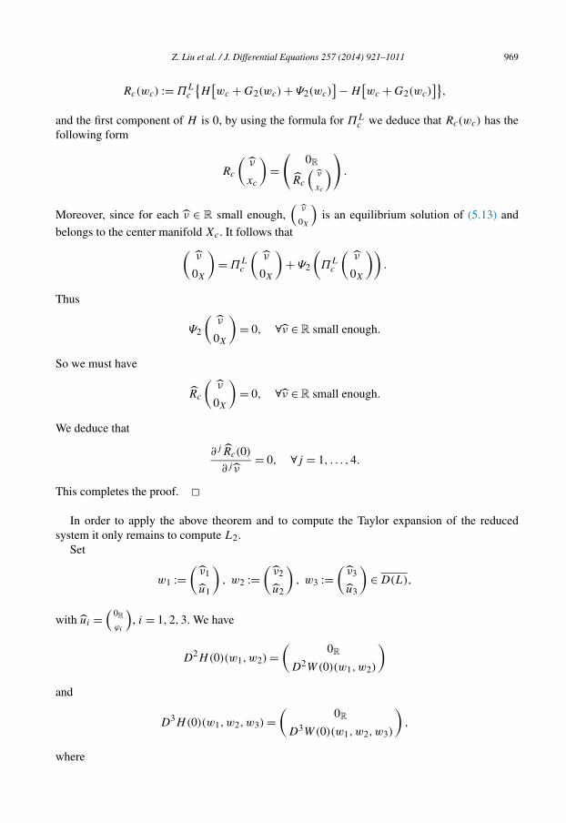
Z. Liu et al. / J. Differential Equations 257 (2014) 921–1011 969
Rc(wc) := ΠLc
{H[wc + G2(wc) + Ψ2(wc)
]− H[wc + G2(wc)
]},
and the first component of H is 0, by using the formula for ΠLc we deduce that Rc(wc) has the
following form
Rc
(ν
xc
)=(
0R
Rc
(ν
xc
)) .
Moreover, since for each ν ∈ R small enough,(
ν
0X
)is an equilibrium solution of (5.13) and
belongs to the center manifold Xc. It follows that(ν
0X
)= ΠL
c
(ν
0X
)+ Ψ2
(ΠL
c
(ν
0X
)).
Thus
Ψ2
(ν
0X
)= 0, ∀ν ∈ R small enough.
So we must have
Rc
(ν
0X
)= 0, ∀ν ∈R small enough.
We deduce that
∂j Rc(0)
∂j ν= 0, ∀j = 1, . . . , 4.
This completes the proof. �In order to apply the above theorem and to compute the Taylor expansion of the reduced
system it only remains to compute L2.Set
w1 :=(
ν1
u1
), w2 :=
(ν2
u2
), w3 :=
(ν3
u3
)∈ D(L),
with ui =(
0Rϕi
), i = 1, 2, 3. We have
D2H(0)(w1,w2) =(
0RD2W(0)(w1,w2)
)and
D3H(0)(w1,w2,w3) =(
0RD3W(0)(w1,w2,w3)
),
where
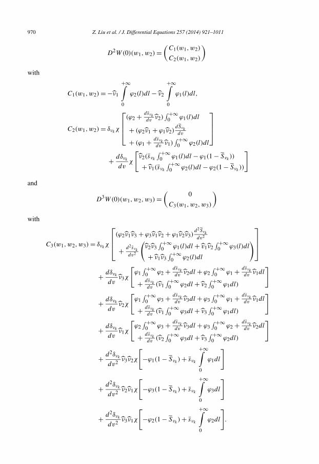
970 Z. Liu et al. / J. Differential Equations 257 (2014) 921–1011
D2W(0)(w1,w2) =(
C1(w1,w2)
C2(w1,w2)
)with
C1(w1,w2) = −ν1
+∞∫0
ϕ2(l)dl − ν2
+∞∫0
ϕ1(l)dl,
C2(w1,w2) = δνkχ
⎡⎢⎢⎣(ϕ2 + dsνk
dvν2)∫ +∞
0 ϕ1(l)dl
+ (ϕ2ν1 + ϕ1ν2)dSνk
dv
+ (ϕ1 + dsνk
dvν1)∫ +∞
0 ϕ2(l)dl
⎤⎥⎥⎦+ dδνk
dvχ
[ν2(sνk
∫ +∞0 ϕ1(l)dl − ϕ1(1 − Sνk
))
+ ν1(sνk
∫ +∞0 ϕ2(l)dl − ϕ2(1 − Sνk
))
]
and
D3W(0)(w1,w2,w3) =(
0
C3(w1,w2,w3)
)with
C3(w1,w2,w3) = δνkχ
⎡⎢⎢⎣(ϕ2ν1ν3 + ϕ3ν1ν2 + ϕ1ν2ν3)
d2Sνk
dv2
+ d2sνk
dv2
(ν2ν3
∫ +∞0 ϕ1(l)dl + v1ν2
∫ +∞0 ϕ3(l)dl
+ ν1ν3∫ +∞
0 ϕ2(l)dl
)⎤⎥⎥⎦
+ dδνk
dvν3χ
[ϕ1∫ +∞
0 ϕ2 + dsνk
dvν2dl + ϕ2
∫ +∞0 ϕ1 + dsνk
dvν1dl
+ dsνk
dv(ν1∫ +∞
0 ϕ2dl + ν2∫ +∞
0 ϕ1dl)
]
+ dδνk
dvν2χ
[ϕ1∫ +∞
0 ϕ3 + dsνk
dvν3dl + ϕ3
∫ +∞0 ϕ1 + dsνk
dvν1dl
+ dsνk
dv(ν1∫ +∞
0 ϕ3dl + ν3∫ +∞
0 ϕ1dl)
]
+ dδνk
dvν1χ
[ϕ2∫ +∞
0 ϕ3 + dsνk
dvν3dl + ϕ3
∫ +∞0 ϕ2 + dsνk
dvν2dl
+ dsνk
dv(ν2∫ +∞
0 ϕ3dl + ν3∫ +∞
0 ϕ2dl)
]
+ d2δνk
dv2ν3ν2χ
[−ϕ1(1 − Sνk
) + sνk
+∞∫0
ϕ1dl
]
+ d2δνk
dv2ν2ν1χ
[−ϕ3(1 − Sνk
) + sνk
+∞∫0
ϕ3dl
]
+ d2δνk
dv2ν3ν1χ
[−ϕ2(1 − Sνk
) + sνk
+∞∫ϕ2dl
].
0

Z. Liu et al. / J. Differential Equations 257 (2014) 921–1011 971
Next recall that
d
dt
[L2(eLctw1, eLctw2
)](0) = L2(Lcw1,w2) + L2(w1,Lcw2).
So system (5.12) can be rewritten as
L2(Lcw1,w2) + L2(w1,Lcw2) = LhL2(w1,w2) + 1
2!ΠhD2H(0)(w1,w2). (5.15)
(i) Computation of L2(e1, e1). We have
ΠhD2H(0)(e1, e1) = 0, Lce1 = 0.
So the equation
L2(Lce1, e1) + L2(e1,Lce1) = LhL2(e1, e1) + 1
2!ΠhD2H(0)(e1, e1)
is equivalent to
0 = LhL2(e1, e1).
Since 0 belongs to the resolvent set of Lh, we obtain that
L2(e1, e1) = 0. (5.16)
(ii) Computation of L2(e1, e2). We have
D2H(0)(e1, e2) =( 0(
− ∫ +∞0 b1(l)dl
Θ1,2
))
with
Θ1,2 = δνkχ
[b1
dSνk
dv+ dsνk
dv
+∞∫0
b1(l)dl
]
+ dδνk
dvχ
[sνk
+∞∫0
b1(l)dl − b1(1 − Sνk)
]
and
Lce1 = 0, Lce2 = iωke2.
So in this case system (5.15) becomes
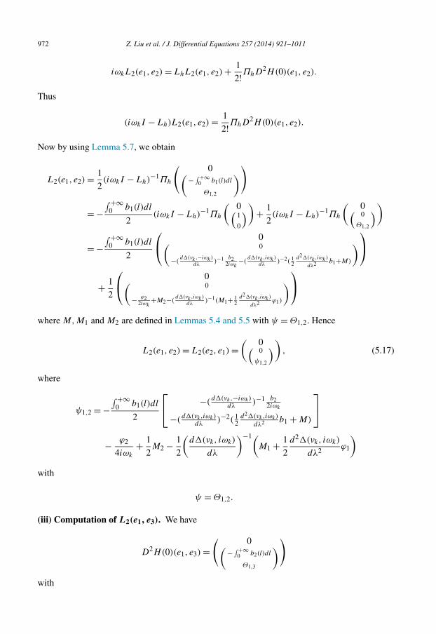
972 Z. Liu et al. / J. Differential Equations 257 (2014) 921–1011
iωkL2(e1, e2) = LhL2(e1, e2) + 1
2!ΠhD2H(0)(e1, e2).
Thus
(iωkI − Lh)L2(e1, e2) = 1
2!ΠhD2H(0)(e1, e2).
Now by using Lemma 5.7, we obtain
L2(e1, e2) = 1
2(iωkI − Lh)−1Πh
( 0(− ∫ +∞
0 b1(l)dl
Θ1,2
))
= −∫ +∞
0 b1(l)dl
2(iωkI − Lh)−1Πh
( 0(1
0
))+ 1
2(iωkI − Lh)−1Πh
( 0(0
Θ1,2
))
= −∫ +∞
0 b1(l)dl
2
⎛⎝ 0( 0
−(d�(νk ,−iωk)
dλ)−1 b2
2iωk−(
d�(νk ,iωk)
dλ)−2( 1
2d2�(νk,iωk)
dλ2 b1+M)
)⎞⎠+ 1
2
⎛⎝ 0( 0
− ϕ22iωk
+M2−(d�(νk ,iωk)
dλ)−1(M1+ 1
2d2�(νk,iωk)
dλ2 ϕ1)
)⎞⎠where M,M1 and M2 are defined in Lemmas 5.4 and 5.5 with ψ = Θ1,2. Hence
L2(e1, e2) = L2(e2, e1) =( 0(
0
ψ1,2
)), (5.17)
where
ψ1,2 = −∫ +∞
0 b1(l)dl
2
⎡⎣ −(d�(νk,−iωk)
dλ)−1 b2
2iωk
−(d�(νk,iωk)
dλ)−2( 1
2d2�(νk,iωk)
dλ2 b1 + M)
⎤⎦− ϕ2
4iωk
+ 1
2M2 − 1
2
(d�(νk, iωk)
dλ
)−1(M1 + 1
2
d2�(νk, iωk)
dλ2ϕ1
)with
ψ = Θ1,2.
(iii) Computation of L2(e1, e3). We have
D2H(0)(e1, e3) =( 0(
− ∫ +∞0 b2(l)dl
Θ1,3
))
with

Z. Liu et al. / J. Differential Equations 257 (2014) 921–1011 973
Θ1,3 = δνkχ
[b2
dSνk
dv+ dsνk
dv
+∞∫0
b2(l)dl
]
+ dδνk
dvχ
[sνk
+∞∫0
b2(l)dl − b2(1 − Sνk)
]
and
Lce1 = 0, Lce3 = −iωke3.
In this case system (5.15) becomes
−iωkL2(e1, e3) = LhL2(e1, e3) + 1
2!ΠhD2H(0)(e1, e3).
So
(−iωkI − Lh)L2(e1, e3) = 1
2!ΠhD2H(0)(e1, e3).
Thus, by Lemma 5.7 we have
L2(e1, e3) = 1
2(−iωkI − Lh)−1Πh
( 0(− ∫ +∞
0 b2(l)dl
Θ1,3
))
= −∫ +∞
0 b2(l)dl
2(−iωkI − Lh)−1Πh
( 0(1
0
))+ 1
2(−iωkI − Lh)−1Πh
( 0(0
Θ1,3
))
= −∫ +∞
0 b2(l)dl
2
⎛⎝ 0( 0
d�(νk,iωk)
dλ
−1 b12iωk
−(d�(νk ,−iωk)
dλ)−2( 1
2d2�(νk,−iωk)
dλ2 b2+N)
)⎞⎠+ 1
2
⎛⎝ 0( 0
ϕ12iωk
+N2−(d�(νk ,−iωk)
dλ)−1(N1+ 1
2d2�(νk,−iωk)
dλ2 ϕ2)
)⎞⎠where N,N1 and N2 are defined in Lemmas 5.4 and 5.5 with ψ = Θ1,3. Then
L2(e1, e3) = L2(e3, e1) =( 0(
0
ψ1,3
)), (5.18)
where
ψ1,3 = −∫ +∞
0 b2(l)dl
2
[(d�(νk, iωk)
dλ
)−1b1
2iωk
−(
d�(νk,−iωk))−2(1 d2�(νk,−iωk)
2b2 + N
)]
dλ 2 dλ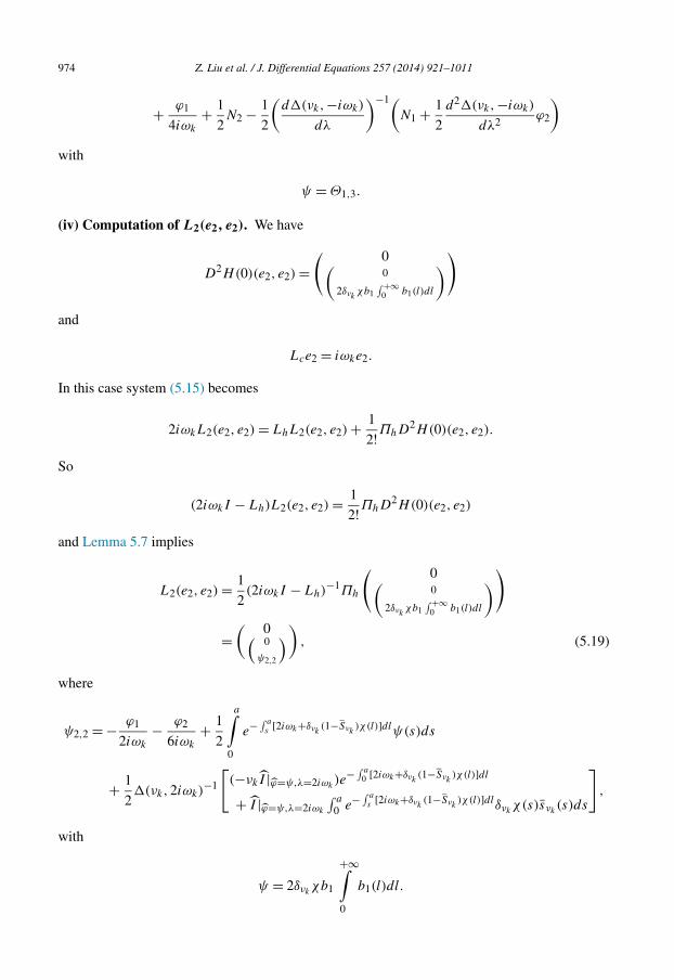
974 Z. Liu et al. / J. Differential Equations 257 (2014) 921–1011
+ ϕ1
4iωk
+ 1
2N2 − 1
2
(d�(νk,−iωk)
dλ
)−1(N1 + 1
2
d2�(νk,−iωk)
dλ2ϕ2
)with
ψ = Θ1,3.
(iv) Computation of L2(e2, e2). We have
D2H(0)(e2, e2) =( 0(
0
2δνkχb1
∫ +∞0 b1(l)dl
))
and
Lce2 = iωke2.
In this case system (5.15) becomes
2iωkL2(e2, e2) = LhL2(e2, e2) + 1
2!ΠhD2H(0)(e2, e2).
So
(2iωkI − Lh)L2(e2, e2) = 1
2!ΠhD2H(0)(e2, e2)
and Lemma 5.7 implies
L2(e2, e2) = 1
2(2iωkI − Lh)−1Πh
( 0(0
2δνkχb1
∫ +∞0 b1(l)dl
))
=( 0(
0
ψ2,2
)), (5.19)
where
ψ2,2 = − ϕ1
2iωk
− ϕ2
6iωk
+ 1
2
a∫0
e− ∫ as [2iωk+δνk
(1−Sνk)χ(l)]dlψ(s)ds
+ 1
2�(νk, 2iωk)
−1
[(−νkI |ϕ=ψ,λ=2iωk
)e− ∫ a0 [2iωk+δνk
(1−Sνk)χ(l)]dl
+ I |ϕ=ψ,λ=2iωk
∫ a
0 e− ∫ as [2iωk+δνk
(1−Sνk)χ(l)]dlδνk
χ(s)sνk(s)ds
],
with
ψ = 2δνkχb1
+∞∫b1(l)dl.
0
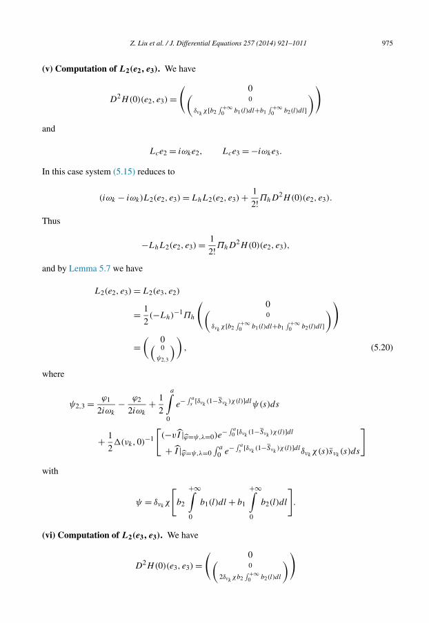
Z. Liu et al. / J. Differential Equations 257 (2014) 921–1011 975
(v) Computation of L2(e2, e3). We have
D2H(0)(e2, e3) =( 0(
0
δνkχ[b2
∫ +∞0 b1(l)dl+b1
∫ +∞0 b2(l)dl]
))
and
Lce2 = iωke2, Lce3 = −iωke3.
In this case system (5.15) reduces to
(iωk − iωk)L2(e2, e3) = LhL2(e2, e3) + 1
2!ΠhD2H(0)(e2, e3).
Thus
−LhL2(e2, e3) = 1
2!ΠhD2H(0)(e2, e3),
and by Lemma 5.7 we have
L2(e2, e3) = L2(e3, e2)
= 1
2(−Lh)−1Πh
( 0(0
δνkχ[b2
∫ +∞0 b1(l)dl+b1
∫ +∞0 b2(l)dl]
))
=( 0(
0
ψ2,3
)), (5.20)
where
ψ2,3 = ϕ1
2iωk
− ϕ2
2iωk
+ 1
2
a∫0
e− ∫ as [δνk
(1−Sνk)χ(l)]dlψ(s)ds
+ 1
2�(νk, 0)−1
[(−vI |ϕ=ψ,λ=0)e− ∫ a
0 [δνk(1−Sνk
)χ(l)]dl
+ I |ϕ=ψ,λ=0∫ a
0 e− ∫ as [δνk
(1−Sνk)χ(l)]dlδνk
χ(s)sνk(s)ds
]
with
ψ = δνkχ
[b2
+∞∫0
b1(l)dl + b1
+∞∫0
b2(l)dl
].
(vi) Computation of L2(e3, e3). We have
D2H(0)(e3, e3) =( 0(
0∫ +∞
))
2δνkχb2 0 b2(l)dl

976 Z. Liu et al. / J. Differential Equations 257 (2014) 921–1011
and
Lce3 = −iωke3.
In this case system (5.15) becomes
−2iωkL2(e3, e3) = LhL2(e3, e3) + 1
2!ΠhD2H(0)(e3, e3).
Hence
(−2iωkI − Lh)L2(e3, e3) = 1
2!ΠhD2H(0)(e3, e3).
It follows from Lemma 5.7 that
L2(e3, e3) = 1
2(−2iωkI − Lh)−1Πh
( 0(0
2δνkχb2
∫ +∞0 b2(l)dl
))
= 1
2
( 0
(−2iωkI − Aνk|Π
Aνkh (X)
)−1ΠAνk
h
(0
2δνkχb2
∫ +∞0 b2(l)dl
))
=( 0(
0
ψ3,3
)), (5.21)
where
ψ3,3 = ϕ1
6iωk
+ ϕ2
2iωk
+ 1
2
a∫0
e− ∫ as [−2iωk+δνk
(1−Sνk)χ(l)]dlψ(s)ds
+ 1
2�(νk,−2iωk)−1
×[
(−νkI |ϕ=ψ,λ=−2iωk)e− ∫ a
0 [−2iωk+δνk(1−Sνk
)χ(l)]dl
+ I |ϕ=ψ,λ=−2iωk
∫ a
0 e− ∫ as [−2iωk+δνk
(1−Sνk)χ(l)]dlδνk
χ(s)sνk(s)ds
]
with
ψ = 2δνkχb2
+∞∫0
b2(l)dl.
Next, we can express the above computations in terms of the following basis of Yc = Πc(Y ):
e1 =(
1( 0R)) , e2 =
(0R(0R)) , e3 =
(0R(0R))
0L1 c1 c2

Z. Liu et al. / J. Differential Equations 257 (2014) 921–1011 977
with
c1 = b1 + b2, c2 = b1 − b2
i. (5.22)
Lemma 5.9. The symmetric and bilinear map L2 : Y 2c → Yh ∩ D(L) is defined by
(a) L2(e1, e1) = 0;(b) L2(e1, e2) and L2(e2, e1) are defined by
L2(e1, e2) = L2(e2, e1) =(
0R(0R
2 Re ψ1,2
)) ;
(c) L2(e1, e3) and L2(e3, e1) are defined by
L2(e1, e3) = L2(e3, e1) =(
0R(0R
2 Im ψ1,2
)) ;
(d) L2(e2, e2) is defined by
L2(e2, e2) =(
0R(0R
2 Re ψ2,2+2ψ2,3
)) ;
(e) L2(e2, e3) and L2(e3, e2) are defined by
L2(e2, e3) = L2(e3, e2) =(
0R(0R
2 Im ψ2,2
)) ;
(f) L2(e3, e3) =(
0R(0R
−2 Re ψ2,2+2ψ2,3
)),
where ψ1,2, ψ2,2, and ψ2,3 are defined in (5.17), (5.19), and (5.20), respectively.
Proof. We use the fact that
e1 = e1, e2 = e2 + e3, and e3 = e2 − e3
i.
(a) By using (5.16), (a) follows.(b) We have
L2(e1, e2) = L2(e1, e2) + L2(e1, e3).
So by using (5.17) and (5.18), we obtain
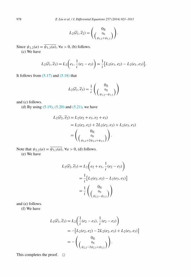
978 Z. Liu et al. / J. Differential Equations 257 (2014) 921–1011
L2(e1, e2) =(
0R(0R
ψ1,2+ψ1,3
)) .
Since ψ1,2(a) = ψ1,3(a), ∀a > 0, (b) follows.(c) We have
L2(e1, e3) = L2
(e1,
1
i(e2 − e3)
)= 1
i
[L2(e1, e2) − L2(e1, e3)
].
It follows from (5.17) and (5.18) that
L2(e1, e3) = 1
i
(0R(0R
ψ1,2−ψ1,3
))
and (c) follows.(d) By using (5.19), (5.20) and (5.21), we have
L2(e2, e2) = L2(e2 + e3, e2 + e3)
= L2(e2, e2) + 2L2(e2, e3) + L2(e3, e3)
=(
0R(0R
ψ2,2+2ψ2,3+ψ3,3
)) .
Note that ψ2,2(a) = ψ3,3(a), ∀a > 0, (d) follows.(e) We have
L2(e2, e3) = L2
(e2 + e3,
1
i(e2 − e3)
)= 1
i
[L2(e2, e2) − L2(e3, e3)
]= 1
i
(0R(0R
ψ2,2−ψ3,3
))
and (e) follows.(f) We have
L2(e3, e3) = L2
(1
i(e2 − e3),
1
i(e2 − e3)
)= −[L2(e2, e2) − 2L2(e2, e3) + L2(e3, e3)
]= −
(0R(0R
ψ2,2−2ψ2,3+ψ3,3
)) .
This completes the proof. �
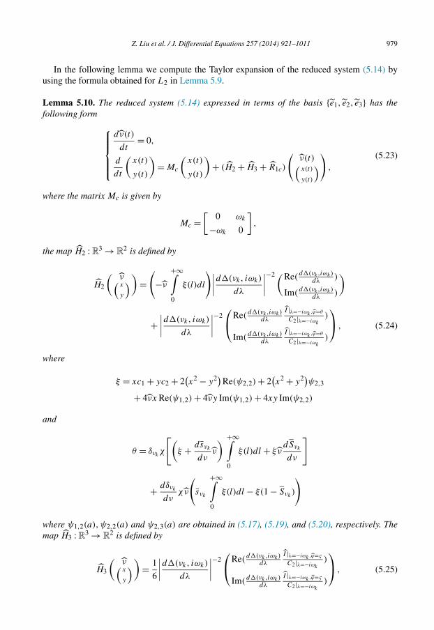
Z. Liu et al. / J. Differential Equations 257 (2014) 921–1011 979
In the following lemma we compute the Taylor expansion of the reduced system (5.14) byusing the formula obtained for L2 in Lemma 5.9.
Lemma 5.10. The reduced system (5.14) expressed in terms of the basis {e1, e2, e3} has thefollowing form ⎧⎪⎪⎪⎨⎪⎪⎪⎩
dν(t)
dt= 0,
d
dt
(x(t)
y(t)
)= Mc
(x(t)
y(t)
)+ (H2 + H3 + R1c)
(ν(t)(x(t)
y(t)
)) ,
(5.23)
where the matrix Mc is given by
Mc =[
0 ωk
−ωk 0
],
the map H2 : R3 →R2 is defined by
H2
(ν(x
y
))=(
−ν
+∞∫0
ξ(l)dl
)∣∣∣∣d�(νk, iωk)
dλ
∣∣∣∣−2(Re(d�(νk,iωk)
dλ)
Im(d�(νk,iωk)
dλ)
)
+∣∣∣∣d�(νk, iωk)
dλ
∣∣∣∣−2⎛⎝Re(
d�(νk,iωk)dλ
I |λ=−iωk ,ϕ=θ
C2|λ=−iωk)
Im(d�(νk,iωk)
dλ
I |λ=−iωk ,ϕ=θ
C2|λ=−iωk)
⎞⎠ , (5.24)
where
ξ = xc1 + yc2 + 2(x2 − y2)Re(ψ2,2) + 2
(x2 + y2)ψ2,3
+ 4νx Re(ψ1,2) + 4νy Im(ψ1,2) + 4xy Im(ψ2,2)
and
θ = δνkχ
[(ξ + dsνk
dνν
) +∞∫0
ξ(l)dl + ξ νdSνk
dν
]
+ dδνk
dνχν
(sνk
+∞∫0
ξ(l)dl − ξ(1 − Sνk)
)
where ψ1,2(a),ψ2,2(a) and ψ2,3(a) are obtained in (5.17), (5.19), and (5.20), respectively. Themap H3 : R3 → R2 is defined by
H3
(ν(x
y
))= 1
6
∣∣∣∣d�(νk, iωk)
dλ
∣∣∣∣−2⎛⎝Re(
d�(νk,iωk)dλ
I |λ=−iωk,ϕ=ς
C2|λ=−iωk)
Im(d�(νk,iωk) I |λ=−iωk,ϕ=ς
)
⎞⎠ , (5.25)
dλ C2|λ=−iωk

980 Z. Liu et al. / J. Differential Equations 257 (2014) 921–1011
with
ς = 3δνkχ
⎡⎣(xc1 + yc2)ν2 d2Sνk
dν2
+ d2sνk
dν2 ν2∫ +∞
0 (xc1 + yc2)(l)dl
⎤⎦+ 6
dδνk
dννχ
[(xc1 + yc2)
∫ +∞0 xc1 + yc2 + dsνk
dννdl
+ dsνk
dνν∫ +∞
0 xc1 + yc2dl
]
+ 3d2δνk
dν2ν2χ
[−(xc1 + yc2)(1 − Sνk
) + sνk
+∞∫0
(xc1 + yc2)dl
], (5.26)
and the remainder term R1c ∈ C4(R3,R2) is given by
R1c
(ν(x
y
))= O
(ν3∥∥∥∥(x
y
)∥∥∥∥+ ν2∥∥∥∥(x
y
)∥∥∥∥2
+ ν
∥∥∥∥(x
y
)∥∥∥∥3
+∥∥∥∥(x
y
)∥∥∥∥4)
. (5.27)
Proof. By using the Taylor expansion of W around 0, the reduced system (5.14) can be rewrittenas follows:
dν(t)
dt= 0,
dxc(t)
dt= (Aνk
)cxc(t) + 1
2!ΠAνkc D2W(0)
((I + G2)
(ν(t)
xc(t)
))2
+ 1
3!ΠAνkc D3W(0)
((I + G2)
(ν(t)
xc(t)
))3
+ R1c
(ν(t)
xc(t)
).
Set
xc =(
0
xc1 + yc2
)=(
0
x(b1 + b2) + y(b1−b2i
)
).
Since {e1, e2, e3} is used as the basis for Yc = Πc(Y ), i.e.,{( 0
c1
),( 0c2
)}is a basis of Xc :=
ΠAνkc (X), we obtain that
Mc =[
0 ωk
−ωk 0
].
(vii) Computation of H2(Y ). We have
(I + G2)
(ν
xc
)= νe1 + xe2 + ye3 + L2(νe1 + xe2 + ye3, νe1 + xe2 + ye3)
= νe1 + xe2 + ye3 + ν2L2(e1, e1) + x2L2(e2, e2) + y2L2(e3, e3)
+ 2νxL2(e1, e2) + 2νyL2(e1, e3) + 2xyL2(e2, e3).

Z. Liu et al. / J. Differential Equations 257 (2014) 921–1011 981
By Lemma 5.9, it follows that
(I + G2)
(ν
xc
)=(
ν(0
ξ
)), (5.28)
where
ξ(a) = xc1(a) + yc2(a) + 2(x2 − y2)Re
(ψ2,2(a)
)+ 2(x2 + y2)ψ2,3(a)
+ 4νx Re(ψ1,2(a)
)+ 4νy Im(ψ1,2(a)
)+ 4xy Im(ψ2,2(a)
).
Then we deduce that
1
2!D2W(0)
((ν(0
ξ
)))2
=(−ν
∫ +∞0 ξ(l)dl
θ
).
By projecting on Xc, using (5.5), (5.8), (5.9), and the same identification as above, we obtain that
1
2!ΠAνkc D2W(0)
((I + G2)
(ν(t)
xc(t)
))2
= ΠAνkc
(−ν∫ +∞
0 ξ(l)dl
θ
)
=(
−ν
+∞∫0
ξ(l)dl
)Π
Aνkc
(1
0
)+ Π
Aνkc
(0
θ
)
=(
−ν
+∞∫0
ξ(l)dl
)∣∣∣∣d�(νk, iωk)
dλ
∣∣∣∣−2( 0
Re(d�(νk,iωk)
dλ)c1 + Im(
d�(νk,iωk)dλ
)c2
)
+(
0
ϕ1|ψ=θ + ϕ2|ψ=θ
),
where c1 and c2 are defined in (5.22), ϕ1 and ϕ2 are defined in (5.8) and (5.9). Note that(0
ϕ1|ψ=θ + ϕ2|ψ=θ
)
=(
0
(d�(νk,iωk)
dλ)−1(
I |λ=iωk ,ϕ=θ
C2|λ=iωk)b1 + (
d�(νk,−iωk)dλ
)−1(I |λ=−iωk ,ϕ=θ
C2|λ=−iωk)b2
)
=∣∣∣∣d�(νk, iωk)
dλ
∣∣∣∣−2(
0
Re(d�(νk,iωk)
dλ
I |λ=−iωk,ϕ=θ
C2|λ=−iωk)c1 + Im(
d�(νk,iωk)dλ
I |λ=−iωk ,ϕ=θ
C2|λ=−iωk)c2
).
Then (5.24) follows.
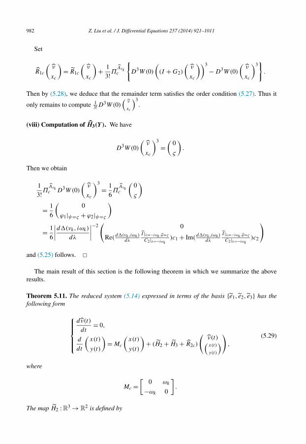
982 Z. Liu et al. / J. Differential Equations 257 (2014) 921–1011
Set
R1c
(ν
xc
)= R1c
(ν
xc
)+ 1
3!ΠAνkc
{D3W(0)
((I + G2)
(ν
xc
))3
− D3W(0)
(ν
xc
)3}
.
Then by (5.28), we deduce that the remainder term satisfies the order condition (5.27). Thus it
only remains to compute 13!D
3W(0)(
ν
xc
)3.
(viii) Computation of H3(Y ). We have
D3W(0)
(ν
xc
)3
=(
0
ς
).
Then we obtain
1
3!ΠAνkc D3W(0)
(ν
xc
)3
= 1
6Π
Aνkc
(0
ς
)= 1
6
(0
ϕ1|ψ=ς + ϕ2|ψ=ς
)
= 1
6
∣∣∣∣d�(νk, iωk)
dλ
∣∣∣∣−2(
0
Re(d�(νk,iωk)
dλ
I |λ=−iωk ,ϕ=ς
C2|λ=−iωk)c1 + Im(
d�(νk,iωk)dλ
I |λ=−iωk ,ϕ=ς
C2|λ=−iωk)c2
)
and (5.25) follows. �The main result of this section is the following theorem in which we summarize the above
results.
Theorem 5.11. The reduced system (5.14) expressed in terms of the basis {e1, e2, e3} has thefollowing form
⎧⎪⎪⎪⎨⎪⎪⎪⎩dν(t)
dt= 0,
d
dt
(x(t)
y(t)
)= Mc
(x(t)
y(t)
)+ (H2 + H3 + R2c)
(ν(t)(x(t)
y(t)
)) ,
(5.29)
where
Mc =[
0 ωk
−ωk 0
].
The map H2 : R3 →R2 is defined by
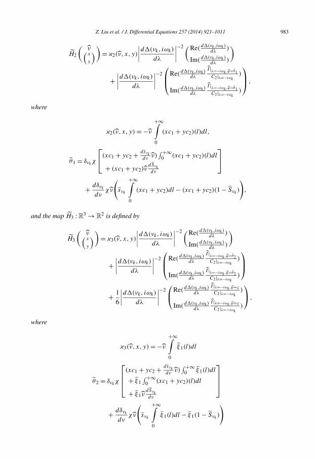
Z. Liu et al. / J. Differential Equations 257 (2014) 921–1011 983
H2
(ν(x
y
))= �2(ν, x, y)
∣∣∣∣d�(νk, iωk)
dλ
∣∣∣∣−2(Re(d�(νk,iωk)
dλ)
Im(d�(νk,iωk)
dλ)
)
+∣∣∣∣d�(νk, iωk)
dλ
∣∣∣∣−2
⎛⎜⎝Re(d�(νk,iωk)
dλ
I |λ=−iωk,ϕ=θ1C2|λ=−iωk
)
Im(d�(νk,iωk)
dλ
I |λ=−iωk,ϕ=θ1C2|λ=−iωk
)
⎞⎟⎠ ,
where
�2(ν, x, y) = −ν
+∞∫0
(xc1 + yc2)(l)dl,
θ1 = δνkχ
⎡⎣(xc1 + yc2 + dsνk
dνν)∫ +∞
0 (xc1 + yc2)(l)dl
+ (xc1 + yc2)νdSνk
dν
⎤⎦+ dδνk
dνχν
(sνk
+∞∫0
(xc1 + yc2)dl − (xc1 + yc2)(1 − Sνk)
),
and the map H3 :R3 → R2 is defined by
H3
(ν(x
y
))= �3(ν, x, y)
∣∣∣∣d�(νk, iωk)
dλ
∣∣∣∣−2(Re(d�(νk,iωk)
dλ)
Im(d�(νk,iωk)
dλ)
)
+∣∣∣∣d�(νk, iωk)
dλ
∣∣∣∣−2
⎛⎜⎝Re(d�(νk,iωk)
dλ
I |λ=−iωk ,ϕ=θ2C2|λ=−iωk
)
Im(d�(νk,iωk)
dλ
I |λ=−iωk ,ϕ=θ2C2|λ=−iωk
)
⎞⎟⎠+ 1
6
∣∣∣∣d�(νk, iωk)
dλ
∣∣∣∣−2⎛⎝Re(
d�(νk,iωk)dλ
I |λ=−iωk ,ϕ=ς
C2|λ=−iωk)
Im(d�(νk,iωk)
dλ
I |λ=−iωk ,ϕ=ς
C2|λ=−iωk)
⎞⎠ ,
where
�3(ν, x, y) = −ν
+∞∫0
ξ1(l)dl
θ2 = δνkχ
⎡⎢⎢⎣(xc1 + yc2 + dsνk
dνν)∫ +∞
0 ξ1(l)dl
+ ξ1∫ +∞
0 (xc1 + yc2)(l)dl
+ ξ1νdSνk
dν
⎤⎥⎥⎦+ dδνk
dνχν
(sνk
+∞∫ξ1(l)dl − ξ1(1 − Sνk
)
)
0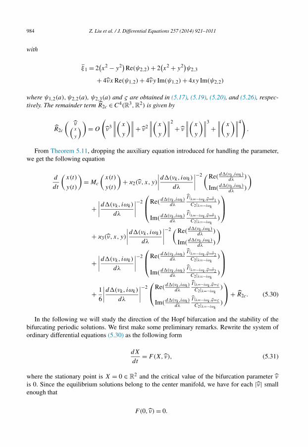
984 Z. Liu et al. / J. Differential Equations 257 (2014) 921–1011
with
ξ1 = 2(x2 − y2)Re(ψ2,2) + 2
(x2 + y2)ψ2,3
+ 4νx Re(ψ1,2) + 4νy Im(ψ1,2) + 4xy Im(ψ2,2)
where ψ1,2(a),ψ2,2(a), ψ2,3(a) and ς are obtained in (5.17), (5.19), (5.20), and (5.26), respec-tively. The remainder term R2c ∈ C4(R3,R2) is given by
R2c
(ν(x
y
))= O
(ν3∥∥∥∥(x
y
)∥∥∥∥+ ν2∥∥∥∥(x
y
)∥∥∥∥2
+ ν
∥∥∥∥(x
y
)∥∥∥∥3
+∥∥∥∥(x
y
)∥∥∥∥4)
.
From Theorem 5.11, dropping the auxiliary equation introduced for handling the parameter,we get the following equation
d
dt
(x(t)
y(t)
)= Mc
(x(t)
y(t)
)+ �2(ν, x, y)
∣∣∣∣d�(νk, iωk)
dλ
∣∣∣∣−2(Re(d�(νk,iωk)
dλ)
Im(d�(νk,iωk)
dλ)
)
+∣∣∣∣d�(νk, iωk)
dλ
∣∣∣∣−2
⎛⎜⎝Re(d�(νk,iωk)
dλ
I |λ=−iωk,ϕ=θ1C2|λ=−iωk
)
Im(d�(νk,iωk)
dλ
I |λ=−iωk,ϕ=θ1C2|λ=−iωk
)
⎞⎟⎠+ �3(ν, x, y)
∣∣∣∣d�(νk, iωk)
dλ
∣∣∣∣−2(Re(d�(νk,iωk)
dλ)
Im(d�(νk,iωk)
dλ)
)
+∣∣∣∣d�(νk, iωk)
dλ
∣∣∣∣−2
⎛⎜⎝Re(d�(νk,iωk)
dλ
I |λ=−iωk,ϕ=θ2C2|λ=−iωk
)
Im(d�(νk,iωk)
dλ
I |λ=−iωk,ϕ=θ2C2|λ=−iωk
)
⎞⎟⎠+ 1
6
∣∣∣∣d�(νk, iωk)
dλ
∣∣∣∣−2⎛⎝Re(
d�(νk,iωk)dλ
I |λ=−iωk ,ϕ=ς
C2|λ=−iωk)
Im(d�(νk,iωk)
dλ
I |λ=−iωk ,ϕ=ς
C2|λ=−iωk)
⎞⎠+ R2c. (5.30)
In the following we will study the direction of the Hopf bifurcation and the stability of thebifurcating periodic solutions. We first make some preliminary remarks. Rewrite the system ofordinary differential equations (5.30) as the following form
dX
dt= F(X, ν), (5.31)
where the stationary point is X = 0 ∈ R2 and the critical value of the bifurcation parameter ν
is 0. Since the equilibrium solutions belong to the center manifold, we have for each |ν| smallenough that
F(0, ν) = 0.

Z. Liu et al. / J. Differential Equations 257 (2014) 921–1011 985
One may observe that ∂xF (0, ν) is unknown whenever ν �= 0. System (5.29) only provides anapproximation at the order 2 of ∂xF (0, ν) with respect to ν. Nevertheless by using Proposi-tion 4.22 in Magal and Ruan [43], we know that the eigenvalues λ(ν) of ∂xF (0, ν) are the rootsof the original characteristic equation
0 = �(ν,λ) = 1 − e−λ + λ2
νh(ν)+ λ
ν
⇔ 0 = �1(ν, λ) := λ[λ + νκ(c)
]+ ν2κ(c)(1 − e−λ
)⇔ 0 = �1(ν + νk, λ) := λ
[λ + (ν + νk)κ(c)
]+ (ν + νk
)2κ(c)
(1 − e−λ
),
λ ∈ Ω, κ(c) = ( 1c)2
1 −√
1 − 1c2
and
λ(0) = ±iωk.
From Proposition 5.1, we know that for c ≥ 1 the characteristic equation has a unique pair of
complex conjugate roots λ(ν), λ(ν) close to iωk,−iωk for ν in a neighborhood of 0. Here λ(ν) =α(ν) + iω(ν), α(0) = 0 and iω(0) = iωk and
α′(0) > 0.
The spectrum of ∂xF (0, ν) is
σ(∂xF (0, ν)
)= {λn(ν), λn(ν)}.
By using a standard procedure (see for example the proof of Lemma 3.3 on page 92 inKuznetsov [34]) and by introducing a complex variable z, system (5.31) can be written for suffi-ciently small |ν| as a single equation:
·z = λ(ν)z + g(z,
−z; ν), (5.32)
where
λ(ν) = α(ν) + iω(ν), g(z,−z, ν) =
3∑i+j=2
1
i!j !gij (ν)zi−zj + O
(|z|3).It is easy to check that (5.31) satisfies
1) F(0, ν) = 0 for ν in an open interval containing 0, and 0 ∈R2 is an isolated stationary pointof F ;
2) F(X, ν) is jointly CL+2(L ≥ 2) in X and ν in a neighborhood of (0, 0) ∈R2 ×R;
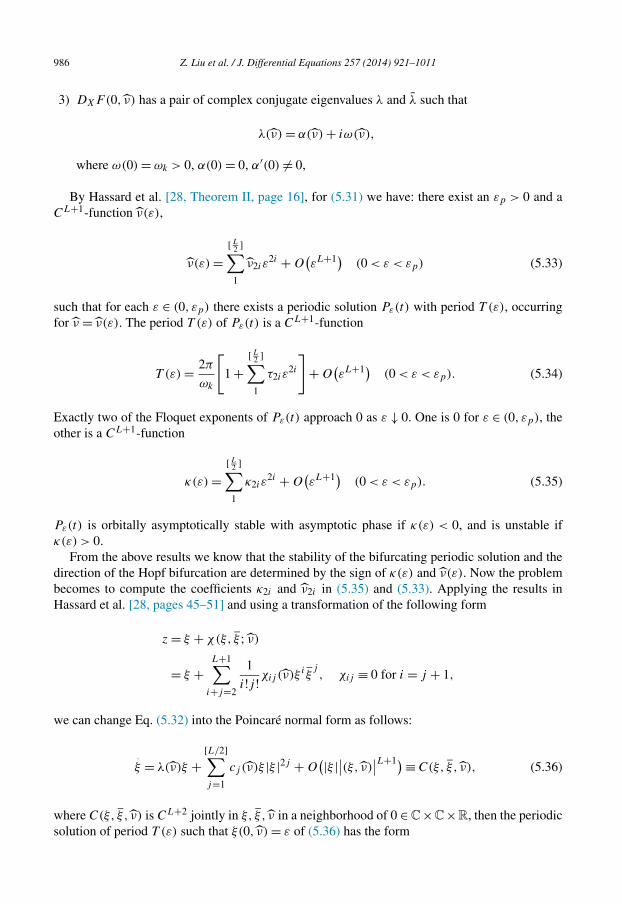
986 Z. Liu et al. / J. Differential Equations 257 (2014) 921–1011
3) DXF(0, ν) has a pair of complex conjugate eigenvalues λ and λ such that
λ(ν) = α(ν) + iω(ν),
where ω(0) = ωk > 0, α(0) = 0, α′(0) �= 0,
By Hassard et al. [28, Theorem II, page 16], for (5.31) we have: there exist an εp > 0 and aCL+1-function ν(ε),
ν(ε) =[ L
2 ]∑1
ν2iε2i + O
(εL+1) (0 < ε < εp) (5.33)
such that for each ε ∈ (0, εp) there exists a periodic solution Pε(t) with period T (ε), occurringfor ν = ν(ε). The period T (ε) of Pε(t) is a CL+1-function
T (ε) = 2π
ωk
[1 +
[ L2 ]∑1
τ2iε2i
]+ O
(εL+1) (0 < ε < εp). (5.34)
Exactly two of the Floquet exponents of Pε(t) approach 0 as ε ↓ 0. One is 0 for ε ∈ (0, εp), theother is a CL+1-function
κ(ε) =[ L
2 ]∑1
κ2iε2i + O
(εL+1) (0 < ε < εp). (5.35)
Pε(t) is orbitally asymptotically stable with asymptotic phase if κ(ε) < 0, and is unstable ifκ(ε) > 0.
From the above results we know that the stability of the bifurcating periodic solution and thedirection of the Hopf bifurcation are determined by the sign of κ(ε) and ν(ε). Now the problembecomes to compute the coefficients κ2i and ν2i in (5.35) and (5.33). Applying the results inHassard et al. [28, pages 45–51] and using a transformation of the following form
z = ξ + χ(ξ, ξ ; ν)
= ξ +L+1∑
i+j=2
1
i!j !χij (ν)ξ iξj, χij ≡ 0 for i = j + 1,
we can change Eq. (5.32) into the Poincaré normal form as follows:
·ξ = λ(ν)ξ +
[L/2]∑j=1
cj (ν)ξ |ξ |2j + O(|ξ |∣∣(ξ, ν)
∣∣L+1)≡ C(ξ, ξ, ν), (5.36)
where C(ξ, ξ, ν) is CL+2 jointly in ξ, ξ, ν in a neighborhood of 0 ∈C×C×R, then the periodicsolution of period T (ε) such that ξ(0, ν) = ε of (5.36) has the form
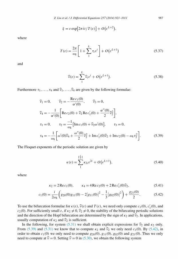
Z. Liu et al. / J. Differential Equations 257 (2014) 921–1011 987
ξ = ε exp[2πit/T (ε)
]+ O(εL+2),
where
T (ε) = 2π
ωk
[1 +
L∑1
τiεi
]+ O
(εL+1) (5.37)
and
ν(ε) =L∑1
νiεi + O
(εL+1). (5.38)
Furthermore τ1, . . . , τ4 and ν1, . . . , ν4 are given by the following formulae:
ν1 = 0, ν2 = −Re c1(0)
α′(0), ν3 = 0,
ν4 = − 1
α′(0)
[Re c2(0) + ν2 Re c′
1(0) + α′′(0)
2ν2
2
],
τ1 = 0, τ2 = −1
ωk
[Im c1(0) + ν2ω′(0)
], τ3 = 0,
τ4 = − 1
ωk
[ω′(0)ν4 + ω′′(0)
2ν2
2 + Im c′1(0)ν2 + Im c2(0) − ωkτ
22
]. (5.39)
The Floquet exponents of the periodic solution are given by
κ(ε) =[ L
2 ]∑1
κ2iε2i + O
(εL+1), (5.40)
where
κ2 = 2 Re c1(0), κ4 = 4 Re c2(0) + 2 Re c′1(0)ν2, (5.41)
c1(0) = i
2ωk
(g20(0)g11(0) − 2
∣∣g11(0)∣∣2 − 1
3
∣∣g02(0)∣∣2)+ g21(0)
2. (5.42)
To use the bifurcation formulae for κ(ε), ν(ε) and T (ε), we need only compute c1(0), c′1(0), and
c2(0). For sufficiently small ε, if κ2 �= 0, ν2 �= 0, the stability of the bifurcating periodic solutionsand the direction of the Hopf bifurcation are determined by the sign of κ2 and ν2. In applications,usually computation of κ2 and v2 is sufficient.
In the following, for system (5.31) we shall obtain explicit expressions for ν2 and κ2 only.From (5.39) and (5.31) we know that to compute κ2 and ν2 we only need c1(0). By (5.42), inorder to obtain c1(0) we only need to compute g20(0), g11(0), g02(0) and g21(0). Thus we onlyneed to compute at ν = 0. Setting ν = 0 in (5.30), we obtain the following system

988 Z. Liu et al. / J. Differential Equations 257 (2014) 921–1011
d
dt
(x(t)
y(t)
)= Mc
(x(t)
y(t)
)+∣∣∣∣d�(νk, iωk)
dλ
∣∣∣∣−2⎛⎝Re(
d�(νk,iωk)dλ
I |λ=−iωk ,ϕ=θ1C2|λ=−iωk
)
Im(d�(νk,iωk)
dλ
I |λ=−iωk ,ϕ=θ1C2|λ=−iωk
)
⎞⎠
+∣∣∣∣d�(νk, iωk)
dλ
∣∣∣∣−2⎛⎝Re(
d�(νk,iωk)dλ
I |λ=−iωk ,ϕ=θ2C2|λ=−iωk
)
Im(d�(νk,iωk)
dλ
I |λ=−iωk ,ϕ=θ2C2|λ=−iωk
)
⎞⎠+ R2c, (5.43)
where
θ1 = δνkχ
[(xc1 + yc2)
+∞∫0
(xc1 + yc2)(l)dl
],
θ2 = δνkχ
[(xc1 + yc2)
∫ +∞0 ξ1(l)dl
+ ξ1∫ +∞
0 (xc1 + yc2)(l)dl
]
with
ξ1 = 2(x2 − y2)Re(ψ2,2) + 2
(x2 + y2)ψ2,3 + 4xy Im(ψ2,2).
By introducing a complex variable z = y + ix, system (5.43) can be written as a single equation
·z = iωkz(t) + g(z, z),
where g(z, z) is an expansion in powers of z and z:
g(z, z) = g20z2
2+ g11zz + g02
z2
2+ g21
z2z
2+ · · ·
in which
g11 = �1
⎧⎪⎪⎪⎪⎨⎪⎪⎪⎪⎩�2
[(Im I |λ=−iωk,ϕ=θ1)02 + (Im I |λ=−iωk,ϕ=θ1)20
+ i(Re I |λ=−iωk,ϕ=θ1)02 + i(Re I |λ=−iωk,ϕ=θ1)20
]
+ �3
[(Re I |λ=−iωk,ϕ=θ1)02 + (Re I |λ=−iωk,ϕ=θ1)20
−i(Im I |λ=−iωk,ϕ=θ1)02 − i(Im I |λ=−iωk,ϕ=θ1)20
]⎫⎪⎪⎪⎪⎬⎪⎪⎪⎪⎭ ,
g20 = g11 + �, g02 = g11 − �
with
(Re I |λ=−iωk,ϕ=θ1)11 =+∞∫0
a∫0
{cos ωk(a − s)e− ∫ a
s δνk(1−Sνk
)χ(l)dlδνkχ(s)
[c1(s)∫ +∞
0 c2(l)dl + c2(s)∫ +∞
0 c1(l)dl]
}dsda,
(Im I |λ=−iωk,ϕ=θ1)11 =+∞∫ a∫ {
sin ωk(a − s)e− ∫ as δνk
(1−Sνk)χ(l)dlδνk
χ(s)
[c1(s)∫ +∞
0 c2(l)dl + c2(s)∫ +∞
0 c1(l)dl]
}dsda,
0 0
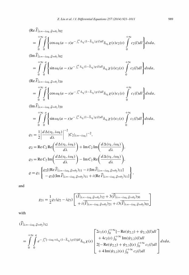
Z. Liu et al. / J. Differential Equations 257 (2014) 921–1011 989
(Re I |λ=−iωk,ϕ=θ1)02
=+∞∫0
a∫0
{cos ωk(a − s)e− ∫ a
s δνk(1−Sνk
)χ(l)dlδνkχ(s)c2(s)
+∞∫0
c2(l)dl
}dsda,
(Im I |λ=−iωk,ϕ=θ1)02
=+∞∫0
a∫0
{sin ωk(a − s)e− ∫ a
s δνk(1−Sνk
)χ(l)dlδνkχ(s)c2(s)
+∞∫0
c2(l)dl
}dsda,
(Re I |λ=−iωk,ϕ=θ1)20
=+∞∫0
a∫0
{cos ωk(a − s)e− ∫ a
s δνk(1−Sνk
)χ(l)dlδνkχ(s)c1(s)
+∞∫0
c1(l)dl
}dsda,
(Im I |λ=−iωk,ϕ=θ1)20
=+∞∫0
a∫0
{sin ωk(a − s)e− ∫ a
s δνk(1−Sνk
)χ(l)dlδνkχ(s)c1(s)
+∞∫0
c1(l)dl
}dsda,
�1 = 1
2
∣∣∣∣d�(νk, iωk)
dλ
∣∣∣∣−2
|C2|λ=−iωk|−2,
�2 = Re C2 Re
(d�(νk, iωk)
dλ
)+ Im C2 Im
(d�(νk, iωk)
dλ
),
�3 = Re C2 Im
(d�(νk, iωk)
dλ
)− Im C2 Re
(d�(νk, iωk)
dλ
),
� = �1
{�2[(Re I |λ=−iωk,ϕ=θ2)11 − i(Im I |λ=−iωk,ϕ=θ2)11]− �3[(Im I |λ=−iωk,ϕ=θ2)11 + i(Re I |λ=−iωk,ϕ=θ2)11]
},
and
g21 = 1
2�1(�2 − i�3)
[(I |λ=−iωk,ϕ=θ2)12 + 3(I |λ=−iωk,ϕ=θ2)30
+ i(I |λ=−iωk,ϕ=θ2)21 + i3(I |λ=−iωk,ϕ=θ2)03
]
with
(I |λ=−iωk,ϕ=θ2)12
=+∞∫0
a∫0
e− ∫ as [−iωk+δνk
(1−Sνk)χ(l)]dlδνk
χ(s)
⎡⎢⎢⎢⎢⎣2c1(s)
∫ +∞0 [−Re(ψ2,2) + ψ2,3](l)dl
+ 4c2(s)∫ +∞
0 Im(ψ2,2)(l)dl
2[−Re(ψ2,2) + ψ2,3](s)∫ +∞
0 c1(l)dl
+ 4 Im(ψ2,2)(s)∫ +∞
0 c2(l)dl
⎤⎥⎥⎥⎥⎦dsda,
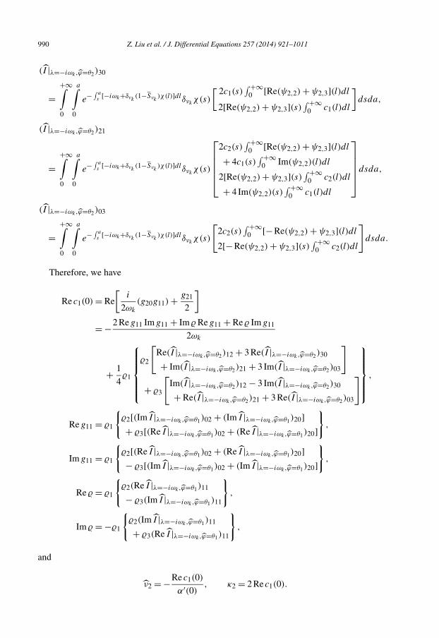
990 Z. Liu et al. / J. Differential Equations 257 (2014) 921–1011
(I |λ=−iωk,ϕ=θ2)30
=+∞∫0
a∫0
e− ∫ as [−iωk+δνk
(1−Sνk)χ(l)]dlδνk
χ(s)
[ 2c1(s)∫ +∞
0 [Re(ψ2,2) + ψ2,3](l)dl
2[Re(ψ2,2) + ψ2,3](s)∫ +∞
0 c1(l)dl
]dsda,
(I |λ=−iωk,ϕ=θ2)21
=+∞∫0
a∫0
e− ∫ as [−iωk+δνk
(1−Sνk)χ(l)]dlδνk
χ(s)
⎡⎢⎢⎢⎢⎣2c2(s)
∫ +∞0 [Re(ψ2,2) + ψ2,3](l)dl
+ 4c1(s)∫ +∞
0 Im(ψ2,2)(l)dl
2[Re(ψ2,2) + ψ2,3](s)∫ +∞
0 c2(l)dl
+ 4 Im(ψ2,2)(s)∫ +∞
0 c1(l)dl
⎤⎥⎥⎥⎥⎦dsda,
(I |λ=−iωk,ϕ=θ2)03
=+∞∫0
a∫0
e− ∫ as [−iωk+δνk
(1−Sνk)χ(l)]dlδνk
χ(s)
[2c2(s)
∫ +∞0 [−Re(ψ2,2) + ψ2,3](l)dl
2[−Re(ψ2,2) + ψ2,3](s)∫ +∞
0 c2(l)dl
]dsda.
Therefore, we have
Re c1(0) = Re
[i
2ωk
(g20g11) + g21
2
]= −2 Re g11 Im g11 + Im � Re g11 + Re � Im g11
2ωk
+ 1
4�1
⎧⎪⎪⎪⎪⎨⎪⎪⎪⎪⎩�2
[Re(I |λ=−iωk,ϕ=θ2)12 + 3 Re(I |λ=−iωk,ϕ=θ2)30
+ Im(I |λ=−iωk,ϕ=θ2)21 + 3 Im(I |λ=−iωk,ϕ=θ2)03
]
+ �3
[Im(I |λ=−iωk,ϕ=θ2)12 − 3 Im(I |λ=−iωk,ϕ=θ2)30
+ Re(I |λ=−iωk,ϕ=θ2)21 + 3 Re(I |λ=−iωk,ϕ=θ2)03
]⎫⎪⎪⎪⎪⎬⎪⎪⎪⎪⎭ ,
Re g11 = �1
{�2[(Im I |λ=−iωk,ϕ=θ1)02 + (Im I |λ=−iωk,ϕ=θ1)20]+ �3[(Re I |λ=−iωk,ϕ=θ1)02 + (Re I |λ=−iωk,ϕ=θ1)20]
},
Im g11 = �1
{�2[(Re I |λ=−iωk,ϕ=θ1)02 + (Re I |λ=−iωk,ϕ=θ1)20]− �3[(Im I |λ=−iωk,ϕ=θ1)02 + (Im I |λ=−iωk,ϕ=θ1)20]
},
Re � = �1
{�2(Re I |λ=−iωk,ϕ=θ1)11
− �3(Im I |λ=−iωk,ϕ=θ1)11
},
Im � = −�1
{�2(Im I |λ=−iωk,ϕ=θ1)11
+ �3(Re I |λ=−iωk,ϕ=θ1)11
},
and
ν2 = −Re c1(0)
′ , κ2 = 2 Re c1(0).
α (0)
Z. Liu et al. / J. Differential Equations 257 (2014) 921–1011 991
For the symmetric case (ii) in Proposition 5.1, we only need to replace νk and ωk by νk and ωk ,respectively in the expression of Re c1(0). From the above discussion we can state the followingresult.
Theorem 5.12. The direction of the Hopf bifurcation is determined by the sign of ν2: if ν2 > 0(< 0), then the bifurcating periodic solutions exist for ν > νk (ν < νk). The periodic solutionsare stable (unstable) if κ2 < 0 (> 0).
The existence of Hopf bifurcation in the structured evolutionary epidemiological model ofinfluenza A drift (1.2) obtained in Magal and Ruan [44] and the stability of the bifurcated periodicsolutions given in Theorem 5.12 indicate that influenza A has an intrinsic tendency to oscillatedue to the evolutionary and/or immunological changes of the influenza viruses. This will be veryhelpful in understanding the seasonal occurrence of influenza A, in predicting the epidemics ofspecific influenza A strains, and in designing effective vaccine programs.
5.2. An age structured population model
Now we apply the normal form theory developed in the previous sections to the age structuredpopulation model (1.6). At first, we make the following assumptions.
Assumption 5.13. Assume that μ > 0, α > 0, γ ∈ L∞(0,+∞) is a map defined by
γ (a) = (a − τ)ne−ς(a−τ)1[τ,+∞)(a) ={
(a − τ)ne−ς(a−τ), if a ≥ τ,
0, otherwise,
where τ ≥ 0, ς ≥ 0, n ∈ N, and assume that ς > 0 whenever n ≥ 1. The map h : R → R isdefined by
h(x) = x exp(−βx), ∀x ∈R,
where β > 0.
For the operator A defined by (1.7), we have
ρ(A) = {λ ∈C : Re(λ) > −μ},
and for each λ ∈ ρ(A),
(λI − A)−1(
χ
ψ
)=(
0
ϕ
)
⇔ ϕ(a) = e−(λ+μ)aχ +a∫
0
e−(λ+μ)(a−s)ψ(s)ds.
It is readily checked that
992 Z. Liu et al. / J. Differential Equations 257 (2014) 921–1011
∥∥(λI − A)−1∥∥≤ 1
λ + μ, ∀λ > −μ.
So A is a Hille–Yosida operator. Now we consider A0, the part of A in X0, which is defined by
A0
(0
ϕ
)= A
(0
ϕ
)=(
0
−ϕ′ − μϕ
), ∀
(0
ϕ
)∈ D(A0),
and
D(A0) ={(
0
ϕ
)∈ {0R} × W 1,1((0,+∞),R
) : ϕ(0) = 0
}.
The linear operator A0 is the infinitesimal generator of a strongly continuous semigroup{TA0(t)}t≥0 of bounded linear operators on X0, which is defined by
TA0(t)
(0
ϕ
)=(
0
TA0(t)ϕ
)with
TA0(t)(ϕ)(a) ={
e−μtϕ(a − t), if a − t ≥ 0,
0, otherwise.
Then we consider {SA(t)}t≥0 ⊂ L(X) the integrated semigroup generated by A. That is the fam-
ily of bounded linear operators on X, such that for each x =(
χ
ψ
)∈ X, the map t → SA(t)x is
an integrated solution of the Cauchy problem
dSA(t)x
dt= ASA(t)x + x, for t ≥ 0, and SA(0)x = 0.
Thus, we deduce that
SA(t)
(χ
ψ
)=(
0
L(t)χ
)+
t∫0
TA0(l)
(0
ψ
)dl
with
L(t)(χ)(a) ={
0, if a − t ≥ 0,
e−μaχ, if a − t ≤ 0.
Finally define a convolution
(SA ∗ f )(t) =t∫SA(t − s)f (s)ds
0

Z. Liu et al. / J. Differential Equations 257 (2014) 921–1011 993
for f ∈ L1(0, τ ;X). Then for each f ∈ L1(0, τ ;X), the map t → (SA ∗ f )(t) belongs toC1([0, τ ],X0) ∩ C([0, τ ],D(A)), and
(SA � f )(t) := d
dt(SA ∗ f )(t)
satisfies
(SA � f )(t) = A
t∫0
(SA � f )(l)dl +t∫
0
f (l)dl, ∀t ∈ [0, τ ].
Then the integrated solution of system (1.9) is unique and is given by
v(t) = TA0(t)
(0
ϕ
)+ (SA � αH
(v(.)
))(t), ∀t ≥ 0.
Set
X0+ := {0} × L1+(0,+∞).
The positive equilibrium solution of (1.9) is given for each α > α0 by
vα =(
0
uα
)with uα(a) = C exp(−μa),
where
α0 = 1∫ +∞0 γ (a)e−μada
, and C := ln(α∫ +∞
0 γ (a)e−μada)
β∫ +∞
0 γ (a)e−μada.
The linearized system of (1.9) around vα is
dw(t)
dt= Aw(t) + αDH(vα)w(t) for t ≥ 0, v(t) ∈ X0,
where
αDH(vα)
(0
ϕ
)=(
η(α)∫ +∞
0 γ (a)ϕ(a)da
0
)and
η(α) = αh′( +∞∫
0
γ (a)uα(a)da
)= 1 − ln(α
∫ +∞0 γ (a)e−μada)∫ +∞
0 γ (a)e−μada.
To simplify the notation, we set

994 Z. Liu et al. / J. Differential Equations 257 (2014) 921–1011
Bαx = Ax + αDH(vα)x with D(Bα) = D(A).
In the following we summarize some results obtained in Magal and Ruan [43].
Lemma 5.14. Let Assumption 5.13 be satisfied. Then the linear operator Bα : D(A) ⊂ X → X
is a Hille–Yosida operator and
ωess((Bα)0
)≤ −μ.
Set
Ω := {λ ∈C : Re(λ) > −μ}.
By using the above lemma, we deduce that for each λ ∈ Ω ,
λ ∈ σ(Bα) ⇔ �(α,λ) = 0,
where the characteristic function is
�(α,λ) := 1 − η(α)
+∞∫0
γ (a)e−(λ+μ)ada for each λ ∈ Ω.
Moreover, by using the fact that γ (a) = (a − τ)ne−ς(a−τ)1[τ,+∞)(a), for each λ ∈ Ω , the char-acteristic equation
�(α,λ) = 0
is equivalent to
1 = n!η(α)e−(λ+μ)τ
(ς + λ + μ)n+1. (5.44)
In the following, we regard α as the bifurcation parameter and have the following result on Hopfbifurcation in model (1.6) (Magal and Ruan [43]).
Proposition 5.15. Let Assumption 5.13 be satisfied and assume that τ > 0. Then the character-istic equation (5.44) with α = αk , k ∈N \ {0}, has a unique pair of purely imaginary roots ±iωk ,where
1 = n!η(αk)e−μτ
(
√(μ + ς)2 + ω2
k)
and ωk > 0 is the unique solution of
−(
ωτ + (n + 1) arctanω
)= π − 2kπ,
ς + μ
Z. Liu et al. / J. Differential Equations 257 (2014) 921–1011 995
so that the age structured model (1.6) undergoes a Hopf bifurcation at the equilibrium u = uαk.
In particular, a non-trivial periodic solution bifurcates from the equilibrium u = uαk.
In the following we study the direction and stability of the Hopf bifurcation by applying thenormal form theory developed in previous sections to the Cauchy problem (1.9). We first includethe parameter α into the state variable. Consider the system
⎧⎪⎪⎪⎨⎪⎪⎪⎩dα(t)
dt= 0,
dv(t)
dt= Av(t) + α(t)H
(v(t)
),
α(0) = α0 ∈R, v(0) = v0 ∈ X0.
Making a change of variables
v(t) = v(t) + vα,
we obtain the system
⎧⎪⎨⎪⎩dα(t)
dt= 0,
dv(t)
dt= Av(t) + α(t)H
(v(t) + vα
)− α(t)H(vα).
Now setting
α = α + αk,
we obtain
⎧⎪⎨⎪⎩dα(t)
dt= 0,
dv(t)
dt= Av(t) + H (α, v),
(5.45)
where
H (α, v) := (α + αk)[H(v(t) + v(α+αk)
)− H(v(α+αk))].
We have
∂vH (α, v)(w) = (α + αk)DH(v + v(α+αk))(w)
and

996 Z. Liu et al. / J. Differential Equations 257 (2014) 921–1011
∂αH (α, v)(α) = α
{H(v + v(α+αk)) − H(v(α+αk))
+ (α + αk)
[DH(v + v(α+αk))
(dv(α+αk)
dα
)− DH(v(α+αk))
(dv(α+αk)
dα
)]}.
So
∂vH (0, 0) = αkDH(vαk) and ∂αH (0, 0) = 0.
Set
X =R× X, X0 =R× D(A).
Consider the linear operator A : D(A) ⊂X →X defined by
A(
α
v
)=(
0
(A + αkDH(vαk))v
)=(
0
Bαkv
)with
D(A) =R× D(A),
and the map F : D(A) →X defined by
F
(α
v
)=( 0
W(
α
v
)),
where W : D(A) → X is defined by
W
(α
v
):= (α + αk)
[H(v + v(α+αk)) − H(v(α+αk))
]− αkDH(vαk)(v).
Then we have
F
(0
0
)= 0 and DF
(0
0
)= 0.
Now we can reformulate system (5.45) as the following system
dw(t)
dt= Aw(t) + F
(w(t)
), w(0) = w0 ∈ D(A). (5.46)
The following lemmas were obtained in Magal and Ruan [43].
Z. Liu et al. / J. Differential Equations 257 (2014) 921–1011 997
Lemma 5.16. Let Assumption 5.13 be satisfied and assume that τ > 0. Then
σ(Bαk|Πc(X)) = {iωk,−iωk}, σ (Bαk
|(I−Πc)(X)) = σ(Bαk) \ {iωk,−iωk}
with
Πc = Πiωk+ Π−iωk
,
Π±iωk
(δ
ψ
)=(
0d�(α,±iωk)
dλ
−1[δ + ∫ +∞0
∫ +∞s
γ (l)e−(±iωk+μ)(l−s)dlψ(s)ds]e−(±iωk+μ).
)and
Πc
(1
0
)=(
0d�(αk,iωk)
dλ
−1e−(iωk+μ)· + d�(αk,−iωk)
dλ
−1e−(−iωk+μ)·
).
Observe that by construction we have
Bαk
(0
e−(±iωk+μ).
)=(
0
−( dda
+ μI)e−(±iωk+μ).
)= ±iωk
(0
e−(±iωk+μ).
).
Set
Πh := (I − Πc), Xc := Πc(X), and Xh := Πh(X).
Lemma 5.17. Let Assumption 5.13 be satisfied and assume that τ > 0. Then
σ(A) = σ(Bαk) ∪ {0}.
Moreover, we have for λ ∈ ρ(A) ∩ Ω = Ω \ (σ (Bαk) ∪ {0}) that
(λ −A)−1(
r(δ
ψ
))=( r
λ
(λ − Bαk)−1
(δ
ψ
))
and the eigenvalues 0 and ±iωk of A are simple. The corresponding projectors Π0,Π±iωk:X +
iX → X + iX are defined by
Π0
(r
v
)=(
r
0
), Π±iωk
(r
v
)=(
0
Π±iωkv
), ∀
(r
v
)∈X + iX .
Note that we have
Πiωk(x) = Π−iωk
(x), ∀x ∈X + iX .
In this context, the projectors Πc :X → X and Πh :X → X are defined by

998 Z. Liu et al. / J. Differential Equations 257 (2014) 921–1011
Πc(x) : = (Π0 + Πiωk+ Π−iωk
)(x), ∀x ∈X ,
Πh(x) : = (I − Πc)(x), ∀x ∈X .
We denote
Xc := Πc(X ), Xh := Πh(X ), Ac := A|Xc, Ah := A|Xh
.
Now we have the decomposition
X = Xc ⊕Xh.
Define the basis of Xc by
e1 :=( 1(
0R0C
)), e2 :=
(0R(0Rc1
)) , e3 =:(
0R(0Rc2
))
with
c1 = e−(μ+iωk). and c2 = e−(μ−iωk)..
We have
Ae1 = 0, Ae2 = iωke2, and Ae3 = −iωke3.
Set
w :=(
α
v
)=(
α(0
u
)) ∈ D(A),
Πcv := vc, Πhv := vh wc := Πcw =(
α
Πcv
)=(
α
vc
)and
wh := Πhw = (I − Πc)w =(
0
Πhv
)=(
0
vh
).
Notice that{(
0
c1
),(
0
c2
)}is the basis of Xc. Set
vc =(
0
x1c1 + x2c2
)and
χ :=+∞∫
γ (a)e−μada = n! exp(−μτ)
(μ + ς)n+1.
0

Z. Liu et al. / J. Differential Equations 257 (2014) 921–1011 999
We observe that for each
w1 :=(
α1
v1
), w2 :=
(α2
v2
)∈ D(A)
with vi =(
0Rϕi
), i = 1, 2,
D2W(0)(w1,w2) = D2W(0)
((α1
v1
),
(α2
v2
))= αkD
2H(vαk)(v1, v2) + α2DH(vαk
)(v1) + α1DH(vαk)(v2)
+ α2αkD2H(vαk
)
(v1,
dvα+αk
dα
∣∣∣∣α=0
)+ α1αkD
2H(vαk)
(v2,
dvα+αk
dα
∣∣∣∣α=0
)with
D2H(vαk)
((0
ϕ1
),
(0
ϕ2
))=( β[ln(αkχ)−2]
αkχ
∏2i=1
∫ +∞0 γ (a)ϕi(a)da
0
).
Then
1
2!D2W(0)(w)2 = 1
2!D2W(0)
(α(0
u
))2
=(˜ψ
0
),
where
˜ψ = − α
αkχ
+∞∫0
γ (a)u(a)da + β(ln(αkχ) − 2)
2χ
( +∞∫0
γ (a)u(a)da
)2
.
By projecting on Xc and using Lemma 5.16, we obtain
1
2!ΠcD2W(0)
(α(0
u
))2
= ˜ψΠc
(1
0
)= ˜ψ [ 0
d�(αk,iωk)dλ
−1c1 + d�(αk,−iωk)
dλ
−1c2
].
Now we compute 12!D
2W(0)(wc)2, 1
2!ΠcD2F(0)(wc)
2, 12!ΠhD2F(0)(wc)
2 and 13!D
3W(0)(wc)3
expressed in terms of the basis {e1, e2, e3}. We first obtain that
1
2!D2W(0)(wc)
2 = 1
2!D2W(0)
(α(0
))2
=(
ψ
0
),
x1c1+x2c2

1000 Z. Liu et al. / J. Differential Equations 257 (2014) 921–1011
where
ψ = − α
αkχ
+∞∫0
γ (a)(x1c1 + x2c2)(a)da
+ β(ln(αkχ) − 2)
2χ
( +∞∫0
γ (a)(x1c1 + x2c2)(a)da
)2
.
Thus
1
2!ΠcD2F(0)(wc)
2 =(
012!ΠcD
2W(0)((
α
vc
))2
)=(
0
ψΠc
(10
))
=( 0
ψ
[0
d�(αk,iωk)
dλ
−1c1+ d�(αk,−iωk)
dλ
−1c2
])(5.47)
and
1
2!ΠhD2F(0)(wc)2 = 1
2! (I − Πc)D2F(0)
((α
vc
))2
=( 0
ψ
[1
− d�(αk,iωk)
dλ
−1c1− d�(αk,−iωk)
dλ
−1c2
]). (5.48)
Next we obtain
1
3!D3W(0)(wc)
3 = 1
3!D3W(0)
(α
vc
)3
=(
ψ
0
)with
ψ = 1
(αk)2(1 − ln(αkχ))α2(
x1 + x2
2
)+ 2βχ
αk(1 − ln(αkχ))2α
(x1 + x2
2
)2
+ 4β2(− ln(αkχ) + 3)χ2
3(1 − ln(αkχ))3
(x1 + x2
2
)3
.
By Lemma 5.16, we obtain
1
3!ΠcD3F(0)(wc)
3 =(
013!ΠcD
3W(0)(wc)3
)=( 0
ψΠc
(1
0
))
=( 0
ψ
[0
d�(α ,iω ) −1 d�(α ,−iω ) −1
]). (5.49)
k kdλ
c1+ k kdλ
c2
Z. Liu et al. / J. Differential Equations 257 (2014) 921–1011 1001
In the following we will compute the normal form of system (5.46). DefineΘc
m : V m(Xc,Xc) → V m(Xc,Xc) by
Θcm(Gc) := [Ac,Gc], ∀Gc ∈ V m(Xc,Xc), (5.50)
and Θhm : V m(Xc,Xh ∩ D(A)) → V m(Xc,Xh) by
Θhm(Gh) := [A,Gh], ∀Gh ∈ V m
(Xc,Xh ∩ D(A)
). (5.51)
We decompose V m(Xc,Xc) into the direct sum
V m(Xc,Xc) =Rcm ⊕ Cc
m,
where
Rcm := R
(Θc
m
),
is the range of Θcm, and Cc
m is some complementary space of Rcm into V m(Xc,Xc). Define
Pm : V m(Xc,X ) → V m(Xc,X ) the bounded linear projector satisfying
Pm
(V m(Xc,X )
)=Rcm ⊕ V m(Xc,Xh), and (I −Pm)
(V m(Xc,X )
)= Ccm.
Now we apply the method described in Theorem 4.4 for k = 3 to system (5.46). The mainpoint is to compute G2 ∈ V 2(Xc,D(A)) defined such that
[A,G2](wc) =P2
[1
2!D2F(0)(wc,wc)
]for each wc ∈Xc (5.52)
in order to obtain the normal form because the reduced system is the following
dwc(t)
dt=Acwc(t) + 1
2!ΠcD2F3(0)
(wc(t),wc(t)
)+ 1
3!ΠcD3F3(0)
(wc(t),wc(t),wc(t)
)+ Rc
(wc(t)
)(5.53)
where
1
2!ΠcD2F3(0)(wc,wc) = 1
2!ΠcD2F2(0)(wc,wc)
= 1
2!ΠcD2F(0)(wc,wc) − [Ac,ΠcG2](wc) (5.54)
and
1
3!ΠcD3F3(0)(wc,wc,wc) = 1
3!ΠcD3F2(0)(wc,wc,wc) − Πc[A,G3](wc)
= 1ΠcD
3F2(0)(wc,wc,wc) − [Ac,ΠcG3](wc). (5.55)
3!
1002 Z. Liu et al. / J. Differential Equations 257 (2014) 921–1011
Set
Gm,k := ΠkGm, ∀k = c,h, m ≥ 2.
Recall that (5.52) is equivalent to finding G2,c ∈ V 2(Xc,Xc) and G2,h ∈ V 2(Xc,Xh ∩ D(A))
satisfying
[Ac,G2,c] = ΠcP2
[1
2!D2F(0)(wc,wc)
](5.56)
and
[A,G2,h] = ΠhP2
[1
2!D2F(0)(wc,wc)
]. (5.57)
From (5.55), we know that the third order term 13!ΠcD
3F2(0)(wc,wc,wc) in the equation isneeded after computing the normal form up to the second order. In the following lemma we findthe expression of 1
3!ΠcD3F2(0)(wc,wc,wc).
Lemma 5.18. Let G2 ∈ V 2(Xc,D(A)) be defined in (5.52). Then after the change of variables
w = w + G2(Πcw), (5.58)
system (5.46) becomes (after dropping the bars)
dw(t)
dt=Aw(t) + F2
(w(t)
), w(0) = w0 ∈ D(A),
where
F2(w(t)
)= F(w(t)
)− [A,G2](wc(t)
)+ O(∥∥w(t)
∥∥3).
In particular,
1
3!ΠcD3F2(0)(wc,wc,wc)
= ΠcD2F(0)
(wc,G2(wc)
)+ 1
3!ΠcD3F(0)(wc,wc,wc)
− DG2,c(wc)
[1
2!ΠcD2F(0)(wc,wc) − [Ac,G2,c](wc)
]. (5.59)
Proof. From Proposition 3.8, the first part is obvious. We only need to prove the formula (5.59).Set
wk(t) := Πkw(t), wk(t) := Πkw(t), ∀k = c,h.
We can split the system (5.46) as

Z. Liu et al. / J. Differential Equations 257 (2014) 921–1011 1003
dwc(t)
dt=Acwc(t) + ΠcF
(wc(t) + wh(t)
),
dwh(t)
dt=Ahwh(t) + ΠhF
(wc(t) + wh(t)
).
Note that (5.58) is equivalent to
wc = wc + G2,c(wc), wh = wh + G2,h(wc).
Since dim(Xc) < +∞, we have
·wc(t) = [I + DG2,c
(wc(t)
)]−1[Ac
(wc(t) + G2,c
(wc(t)
))+ ΠcF(w(t) + G2
(wc(t)
))]=Ac
(wc(t) + G2,c
(wc(t)
))+ ΠcF(w(t) + G2
(wc(t)
))− DG2,c
(wc(t)
)[Ac
(wc(t) + G2,c
(wc(t)
))+ ΠcF(w(t) + G2
(wc(t)
))]+ DG2,c
(wc(t)
)DG2,c
(wc(t)
)[Ac(wc(t) + G2,c(wc(t)))
+ ΠcF(w(t) + G2(wc(t)))
]+ O
(∥∥w(t)∥∥4)
.
Hence
ΠcF2(w(t)
)= ΠcF
(w(t) + G2
(wc(t)
))− [Ac,G2,c](wc(t)
)− DG2,c
(wc(t)
)[ΠcF
(w(t) + G2
(wc(t)
))− [Ac,G2,c](wc(t)
)]+ O(∥∥w(t)
∥∥4).
Let wc ∈Xc. It follows that
ΠcF2(wc) = ΠcF(wc + G2(wc)
)− [Ac,G2,c](wc)
− DG2,c(wc)[ΠcF
(wc + G2(wc)
)− [Ac,G2,c](wc)]+ O
(‖wc‖4).Thus we have
ΠcF2(wc) = 1
2!ΠcD2F(0)(wc,wc) − [Ac,G2,c](wc)
+ ΠcD2F(0)
(wc,G2(wc)
)+ 1
3!ΠcD3F(0)(wc,wc,wc)
− DG2,c(wc)
[1
2!ΠcD2F(0)(wc,wc) − [Ac,G2,c](wc)
]+ O
(‖wc‖4).Then (5.59) follows and the proof is complete. �
Set
wc = αe1 + x1e2 + x2e3.
1004 Z. Liu et al. / J. Differential Equations 257 (2014) 921–1011
We shall compute the normal form expressed in terms of the basis {e1, e2, e3}. ConsiderV m(C3,C3) and V m(C3,Xh ∩ D(A)), which denote the linear space of the homogeneous poly-nomials of degree m in 3 real variables, α, x = (x1, x2) with coefficients in C3 and Xh ∩ D(A),respectively. The operators Θc
m and Θhm considered in (5.50) and (5.51) now act in the spaces
V m(C3,C3) and V m(C3,Xh ∩ D(A)), respectively, and satisfy
Θcm(Gm,c)
⎛⎝ α
x1
x2
⎞⎠ = [Ac,Gm,c]⎛⎝ α
x1
x2
⎞⎠= DGm,cAc
⎛⎝ α
x1
x2
⎞⎠−AcGm,c
⎛⎝ α
x1
x2
⎞⎠
=
⎛⎜⎜⎜⎜⎝DxG1
m,c
(α
x1
x2
)Mcx(
Dx
(G2
m,c
G3m,c
)( α
x1
x2
)Mc
(x1
x2
)− Mc
(G2
m,c
G3m,c
)( α
x1
x2
))⎞⎟⎟⎟⎟⎠ ,
Θhm(Gm,h) = [A,Gm,h] = DGm,hAc −AhGm,h,
∀Gm,c
⎛⎝ α
x1
x2
⎞⎠=⎛⎜⎝G1
m,c
G2m,c
G3m,c
⎞⎟⎠⎛⎝ α
x1
x2
⎞⎠ ∈ V m(C3,C3), ∀Gm,h ∈ V m
(C3,Xh ∩ D(A)
)(5.60)
with
Ac =⎡⎣0 0 0
0 iωk 0
0 0 −iωk
⎤⎦ and Mc =[
iωk 0
0 −iωk
].
We define Θcm : V m(C3,C2) → V m(C3,C2) by
Θcm
(G2
m,c
G3m,c
)= Dx
(G2
m,c
G3m,c
)Mc
(x1
x2
)− Mc
(G2
m,c
G3m,c
),
∀(
G2m,c
G3m,c
)∈ V m
(C3,C2). (5.61)
Lemma 5.19. For m ∈ N\{0, 1}, we have the decomposition
V m(C3,C2)= R
(Θc
m
)⊕ N(Θc
m
)(5.62)
and
N(Θc
m
)= span
⎧⎨⎩(
0
xq11 x
q22 αq3
),
(x
q′1
1 xq′2
2 αq′3
0
)∣∣∣q1 − q2 = −1,
q ′1 − q ′
2 = 1, qi, q ′i ∈ N, i = 1, 2, 3
⎫⎬⎭ . (5.63)
Z. Liu et al. / J. Differential Equations 257 (2014) 921–1011 1005
Proof. The canonical basis of V m(C3,C2) is
Φ ={(
xq11 x
q22 αq3
0
),
(0
xq11 x
q22 αq3
)∣∣∣q1 + q2 + q3 = m
}.
Since Mc =[
iωk 0
0 −iωk
], for each
(x
q11 x
q22 αq3
0
),
(0
xq11 x
q22 αq3
)∈ Φ , we have
Θcm
(x
q11 x
q22 αq3
0
)= Dx
(x
q11 x
q22 αq3
0
)Mc
(x1
x2
)− Mc
(x
q11 x
q22 αq3
0
)= iωk(q1 − q2 − 1)
(x
q11 x
q22 αq3
0
)and
Θcm
(0
xq11 x
q22 αq3
)= Dx
(0
xq11 x
q22 αq3
)Mc
(x1
x2
)− Mc
(0
xq11 x
q22 αq3
)= iωk(q1 − q2 + 1)
(0
xq11 x
q22 αq3
).
Hence the operators Θcm defined in (5.61) have diagonal matrix representation in the canonical
basis of V m(C3,C2). Thus, (5.62) and (5.63) hold. �From (5.63), we obtain
N(Θc
2
)= span
{(x1α
0
),
(0
x2α
)},
N(Θc
3
)= span
{(x2
1x2
0
),
(x1α2
0
),
(0
x1x22
),
(0
x2α2
)}. (5.64)
Define P Rm and P N
m : V m(C3,C2) → V m(C3,C2) the bounded linear projectors satisfying
P Rm
(V m(C3,C2))= R
(Θc
m
)and
P Nm
(V m(C3,C2))= N
(Θc
m
).
We are now ready to compute the normal form of the reduced system expressed in terms of thebasis {e1, e2, e3} of Xc. From (5.47), (5.48), (5.56), (5.57), (5.60)–(5.62) and (5.64), we know
that to find G2 ∈ V 2(Xc,D(A)) defined in (5.52) is equivalent to finding G2,c =⎛⎜⎝G1
2,c
G22,c
G32,c
⎞⎟⎠ :=
ΠcG2 ∈ V 2(C3,C3) and G2,h := ΠhG2 ∈ V 2(C3,Xh ∩ D(A)) such that
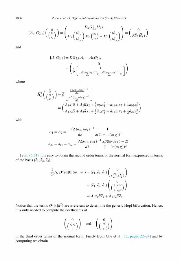
1006 Z. Liu et al. / J. Differential Equations 257 (2014) 921–1011
[Ac,G2,c](
α(x1
x2
))=⎛⎝ DxG1
2,cMcx
Dx
(G2
2,c
G32,c
)Mc
(x1
x2
)− Mc
(G2
2,c
G32,c
)⎞⎠=(
0
P R2 (H 1
2 )
)
and
[A,G2,h] = DG2,hAc −AhG2,h
=( 0
ψ
[1
− d�(αk,iωk)
dλ
−1c1− d�(αk,−iωk)
dλ
−1c2
])
where
H 12
(α(x1
x2
))= ψ
[d�(αk,iωk)
dλ
−1
d�(αk,−iωk)dλ
−1
]
=(
A1x1α + A2αx2 + 12a20x2
1 + a11x1x2 + 12a02x2
2
A1x2α + A2αx1 + 12 a02x2
1 + a11x1x2 + 12 a20x2
2
)with
A1 = A2 = −d�(αk, iωk)
dλ
−1 1
αk(1 − ln(αkχ)),
a20 = a11 = a02 = d�(αk, iωk)
dλ
−1 χβ(ln(αkχ) − 2)
(1 − ln(αkχ))2.
From (5.54), it is easy to obtain the second order terms of the normal form expressed in termsof the basis {e1, e2, e3}:
1
2!ΠcD2F3(0)(wc,wc) = (e1, e2, e3)
(0
P N2 (H 1
2 )
)
= (e1, e2, e3)
(0(
A1x1α
A1x2α
))= A1x1αe2 + A1x2αe3.
Notice that the terms O(|x|α2) are irrelevant to determine the generic Hopf bifurcation. Hence,it is only needed to compute the coefficients of(
0(x2
1 x2
0
)) and
(0( 0
x1x22
))
in the third order terms of the normal form. Firstly from Chu et al. [12, pages 22–24] and bycomputing we obtain
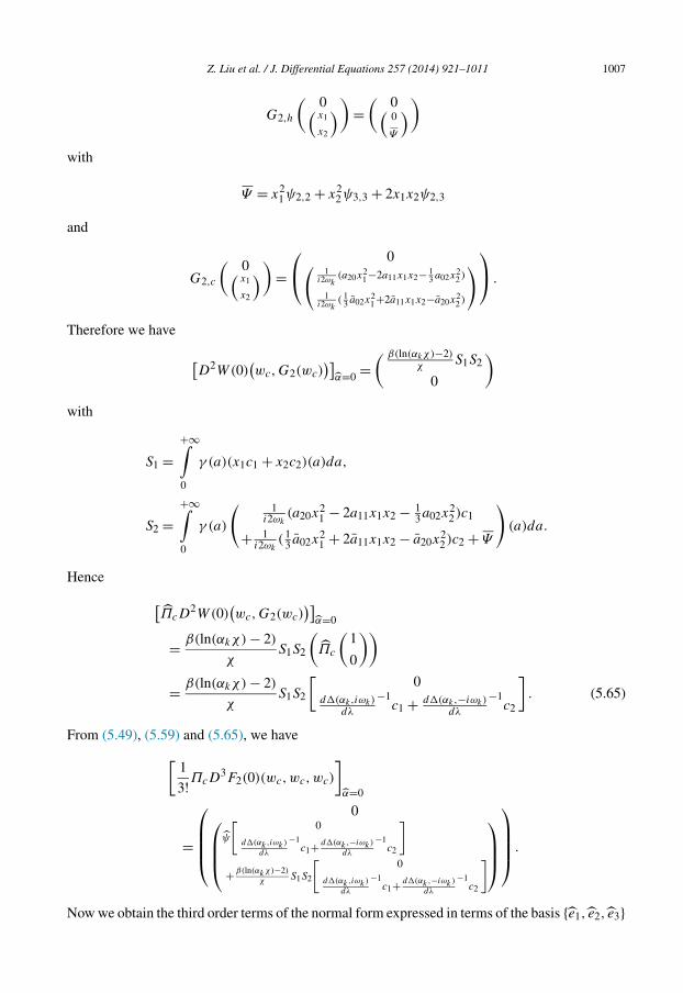
Z. Liu et al. / J. Differential Equations 257 (2014) 921–1011 1007
G2,h
( 0(x1
x2
))=( 0(
0
Ψ
))with
Ψ = x21ψ2,2 + x2
2ψ3,3 + 2x1x2ψ2,3
and
G2,c
( 0(x1
x2
))=⎛⎝ 0(
1i2ωk
(a20x21−2a11x1x2− 1
3 a02x22 )
1i2ωk
( 13 a02x2
1+2a11x1x2−a20x22 )
)⎞⎠ .
Therefore we have
[D2W(0)
(wc,G2(wc)
)]α=0 =
( β(ln(αkχ)−2)χ
S1S2
0
)with
S1 =+∞∫0
γ (a)(x1c1 + x2c2)(a)da,
S2 =+∞∫0
γ (a)
( 1i2ωk
(a20x21 − 2a11x1x2 − 1
3a02x22)c1
+ 1i2ωk
( 13 a02x2
1 + 2a11x1x2 − a20x22)c2 + Ψ
)(a)da.
Hence [ΠcD
2W(0)(wc,G2(wc)
)]α=0
= β(ln(αkχ) − 2)
χS1S2
(Πc
(1
0
))= β(ln(αkχ) − 2)
χS1S2
[0
d�(αk,iωk)dλ
−1c1 + d�(αk,−iωk)
dλ
−1c2
]. (5.65)
From (5.49), (5.59) and (5.65), we have[1
3!ΠcD3F2(0)(wc,wc,wc)
]α=0
=
⎛⎜⎜⎜⎝0⎛⎜⎜⎝ψ
[0
d�(αk,iωk)
dλ
−1c1+ d�(αk,−iωk)
dλ
−1c2
]
+ β(ln(αkχ)−2)
χS1S2
[0
d�(αk,iωk)
dλ
−1c1+ d�(αk,−iωk)
dλ
−1c2
]⎞⎟⎟⎠⎞⎟⎟⎟⎠ .
Now we obtain the third order terms of the normal form expressed in terms of the basis {e1, e2, e3}

1008 Z. Liu et al. / J. Differential Equations 257 (2014) 921–1011
1
3!ΠcD3F3(0)(wc,wc,wc)
= (e1, e2, e3)
⎛⎜⎜⎜⎜⎜⎜⎝
0
P N3
⎛⎜⎜⎜⎜⎜⎝4β2(− ln(αkχ)+3)χ2
3(1−ln(αkχ))3(
x1+x22 )3
⎡⎢⎣ d�(αk,iωk)
dλ
−1
d�(αk,−iωk)
dλ
−1
⎤⎥⎦+⎛⎜⎝ d�(αk,iωk)
dλ
−1 β(ln(αkχ)−2)
χS1S2
d�(αk,−iωk)
dλ
−1 β(ln(αkχ)−2)
χS1S2
⎞⎟⎠
⎞⎟⎟⎟⎟⎟⎠
⎞⎟⎟⎟⎟⎟⎟⎠+ O(|x |α2)
= (e1, e2, e3)
( 0(C1x2
1 x2
C1x1x22
))+ O(|x |α2)
with
C1 =
⎡⎢⎢⎣i
2ωk(a2
11 − 73 |a11|2) + d�(αk,iωk)
dλ
−1 β2(− ln(αkχ)+3)χ2
2(1−ln(αkχ))3
+ d�(αk,iωk)dλ
−1 β(ln(αkχ)−2)1−ln(αkχ)
[∫ +∞0 γ (a)ψ2,2(a)da
+∫ +∞0 γ (a)2ψ2,3(a)da
]⎤⎥⎥⎦ .
Therefore we obtain the following normal form of the reduced system
d
dt
(x1(t)
x2(t)
)= Mc
(x1(t)
x2(t)
)+(
A1x1α
A1x2α
)+(
C1x21x2
C1x1x22
)+ O
(|x |α2 + ∣∣(α, x)∣∣4).
The normal form above can be written in real coordinates (w1,w2) through the change ofvariables x1 = w1 − iw2, x2 = w1 + iw2. Setting w1 = ρ cos ξ , w2 = ρ sin ξ , this normal formbecomes {
ρ = ι1αρ + ι2ρ3 + O(α2ρ + ∣∣(ρ, α)
∣∣4),ξ = −σk + O
(∣∣(ρ, α)∣∣), (5.66)
where
ι1 = Re(A1), ι2 = Re(C1).
Following Chow and Hale [8] we know that the sign of ι1ι2 determines the direction of thebifurcation and that the sign of ι2 determines the stability of the nontrivial periodic orbits. Insummary we have the following theorem.
Theorem 5.20. The flow of (1.6) on the center manifold of the origin at α = αk , k ∈ N+, is givenby (5.66). Furthermore, we have the following
(i) Hopf bifurcation is supercritical if ι1ι2 < 0, and subcritical if ι1ι2 > 0;(ii) the nontrivial periodic solution is stable if ι2 < 0, and unstable if ι2 > 0.
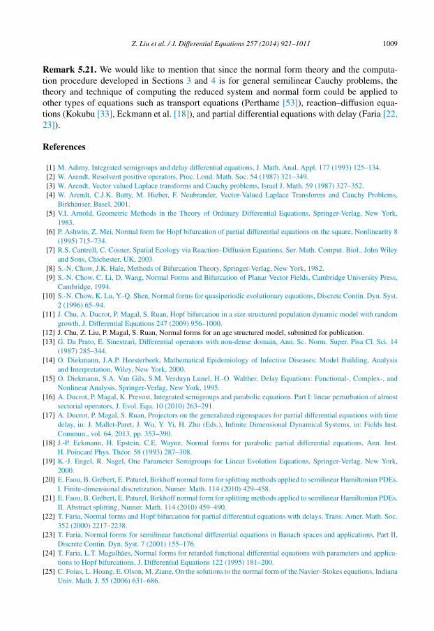
Z. Liu et al. / J. Differential Equations 257 (2014) 921–1011 1009
Remark 5.21. We would like to mention that since the normal form theory and the computa-tion procedure developed in Sections 3 and 4 is for general semilinear Cauchy problems, thetheory and technique of computing the reduced system and normal form could be applied toother types of equations such as transport equations (Perthame [53]), reaction–diffusion equa-tions (Kokubu [33], Eckmann et al. [18]), and partial differential equations with delay (Faria [22,23]).
References
[1] M. Adimy, Integrated semigroups and delay differential equations, J. Math. Anal. Appl. 177 (1993) 125–134.[2] W. Arendt, Resolvent positive operators, Proc. Lond. Math. Soc. 54 (1987) 321–349.[3] W. Arendt, Vector valued Laplace transforms and Cauchy problems, Israel J. Math. 59 (1987) 327–352.[4] W. Arendt, C.J.K. Batty, M. Hieber, F. Neubrander, Vector-Valued Laplace Transforms and Cauchy Problems,
Birkhäuser, Basel, 2001.[5] V.I. Arnold, Geometric Methods in the Theory of Ordinary Differential Equations, Springer-Verlag, New York,
1983.[6] P. Ashwin, Z. Mei, Normal form for Hopf bifurcation of partial differential equations on the square, Nonlinearity 8
(1995) 715–734.[7] R.S. Cantrell, C. Cosner, Spatial Ecology via Reaction–Diffusion Equations, Ser. Math. Comput. Biol., John Wiley
and Sons, Chichester, UK, 2003.[8] S.-N. Chow, J.K. Hale, Methods of Bifurcation Theory, Springer-Verlag, New York, 1982.[9] S.-N. Chow, C. Li, D. Wang, Normal Forms and Bifurcation of Planar Vector Fields, Cambridge University Press,
Cambridge, 1994.[10] S.-N. Chow, K. Lu, Y.-Q. Shen, Normal forms for quasiperiodic evolutionary equations, Discrete Contin. Dyn. Syst.
2 (1996) 65–94.[11] J. Chu, A. Ducrot, P. Magal, S. Ruan, Hopf bifurcation in a size structured population dynamic model with random
growth, J. Differential Equations 247 (2009) 956–1000.[12] J. Chu, Z. Liu, P. Magal, S. Ruan, Normal forms for an age structured model, submitted for publication.[13] G. Da Prato, E. Sinestrari, Differential operators with non-dense domain, Ann. Sc. Norm. Super. Pisa Cl. Sci. 14
(1987) 285–344.[14] O. Diekmann, J.A.P. Heesterbeek, Mathematical Epidemiology of Infective Diseases: Model Building, Analysis
and Interpretation, Wiley, New York, 2000.[15] O. Diekmann, S.A. Van Gils, S.M. Verduyn Lunel, H.-O. Walther, Delay Equations: Functional-, Complex-, and
Nonlinear Analysis, Springer-Verlag, New York, 1995.[16] A. Ducrot, P. Magal, K. Prevost, Integrated semigroups and parabolic equations. Part I: linear perturbation of almost
sectorial operators, J. Evol. Equ. 10 (2010) 263–291.[17] A. Ducrot, P. Magal, S. Ruan, Projectors on the generalized eigenspaces for partial differential equations with time
delay, in: J. Mallet-Paret, J. Wu, Y. Yi, H. Zhu (Eds.), Infinite Dimensional Dynamical Systems, in: Fields Inst.Commun., vol. 64, 2013, pp. 353–390.
[18] J.-P. Eckmann, H. Epstein, C.E. Wayne, Normal forms for parabolic partial differential equations, Ann. Inst.H. Poincaré Phys. Théor. 58 (1993) 287–308.
[19] K.-J. Engel, R. Nagel, One Parameter Semigroups for Linear Evolution Equations, Springer-Verlag, New York,2000.
[20] E. Faou, B. Grébert, E. Paturel, Birkhoff normal form for splitting methods applied to semilinear Hamiltonian PDEs.I. Finite-dimensional discretization, Numer. Math. 114 (2010) 429–458.
[21] E. Faou, B. Grébert, E. Paturel, Birkhoff normal form for splitting methods applied to semilinear Hamiltonian PDEs.II. Abstract splitting, Numer. Math. 114 (2010) 459–490.
[22] T. Faria, Normal forms and Hopf bifurcation for partial differential equations with delays, Trans. Amer. Math. Soc.352 (2000) 2217–2238.
[23] T. Faria, Normal forms for semilinear functional differential equations in Banach spaces and applications, Part II,Discrete Contin. Dyn. Syst. 7 (2001) 155–176.
[24] T. Faria, L.T. Magalhães, Normal forms for retarded functional differential equations with parameters and applica-tions to Hopf bifurcations, J. Differential Equations 122 (1995) 181–200.
[25] C. Foias, L. Hoang, E. Olson, M. Ziane, On the solutions to the normal form of the Navier–Stokes equations, IndianaUniv. Math. J. 55 (2006) 631–686.

1010 Z. Liu et al. / J. Differential Equations 257 (2014) 921–1011
[26] J. Guckenheimer, P. Holmes, Nonlinear Oscillations, Dynamical Systems, and Bifurcations of Vector Fields,Springer-Verlag, New York, 1983.
[27] J.K. Hale, S.M. Verduyn Lunel, Introduction to Functional Differential Equations, Springer-Verlag, New York,1993.
[28] B.D. Hassard, N.D. Kazarinoff, Y.-H. Wan, Theory and Applications of Hopf Bifurcation, London Math. Soc.Lecture Note Ser., vol. 41, Cambridge Univ. Press, Cambridge, 1981.
[29] M. Iannelli, Mathematical Theory of Age-Structured Population Dynamics, Appl. Math. Monogr. C.N.R., vol. 7,Giadini Editori e Stampatori, Pisa, 1994.
[30] H. Inaba, Mathematical analysis for an evolutionary epidemic model, in: M.A. Horn, G. Simonett, G. Webb(Eds.), Mathematical Methods in Medical and Health Sciences, Vanderbilt University Press, Nashville, TN, 1998,pp. 213–236.
[31] H. Inaba, Epidemic threshold and stability in an evolutionary epidemic model, in: C. Castillo-Chavez, et al. (Eds.),Mathematical Approaches for Emerging and Reemerging Infectious Diseases: Models, Methods, and Theory, in:IMA Vol. Math. Appl., vol. 126, Springer, New York, 2002, pp. 337–359.
[32] H. Kellermann, M. Hieber, Integrated semigroups, J. Funct. Anal. 84 (1989) 160–180.[33] H. Kokubu, Normal forms for parametrized vector fields and its application to bifurcations of some reaction diffu-
sion equations, Japan J. Appl. Math. 1 (1984) 273–297.[34] Y.A. Kuznetsov, Elements of Applied Bifurcation Theory, Springer, New York, 1998.[35] Z. Liu, P. Magal, S. Ruan, Projectors on the generalized eigenspaces for functional differential equations using
integrated semigroups, J. Differential Equations 244 (2008) 1784–1809.[36] Z. Liu, P. Magal, S. Ruan, Hopf bifurcation for non-densely defined Cauchy problems, Z. Angew. Math. Phys. 62
(2011) 191–222.[37] Z. Liu, P. Magal, S. Ruan, Center-unstable manifolds for non-densely defined Cauchy problems and applications to
stability of Hopf bifurcation, Can. Appl. Math. Q. 20 (2012) 135–178.[38] Z. Liu, P. Magal, D. Xiao, Bogdanov–Takens bifurcation in a predator prey model with age structure, submitted for
publication.[39] P. Magal, Compact attractors for time-periodic age structured population models, Electron. J. Differential Equations
2001 (2001) 1–35.[40] P. Magal, S. Ruan, On integrated semigroups and age structured models in Lp spaces, Differential Integral Equations
20 (2007) 197–239.[41] P. Magal, S. Ruan (Eds.), Structured Population Models in Biology and Epidemiology, Lecture Notes in Math.,
vol. 1936, Springer, Berlin, 2008.[42] P. Magal, S. Ruan, On semilinear Cauchy problems with non-dense domain, Adv. Differential Equations 14 (2009)
1041–1084.[43] P. Magal, S. Ruan, Center manifolds for semilinear equations with non-dense domain and applications on Hopf
bifurcation in age structured models, Mem. Amer. Math. Soc. 202 (951) (2009).[44] P. Magal, S. Ruan, Sustained oscillations in an evolutionary epidemiological model of influenza A drift, Proc. R.
Soc. Lond. Ser. A Math. Phys. Eng. Sci. 466 (2010) 965–992.[45] H.P. McKean, J. Shatah, The nonlinear Schrödinger equation and the nonlinear heat equation – reduction to linear
form, Comm. Pure Appl. Math. XLIV (1991) 1067–1080.[46] K.R. Meyer, The implicit function theorem and analytic differential equations, in: A. Manning (Ed.), Dynamical
Systems – Warwick 1974, in: Lecture Notes in Math., vol. 468, Springer-Verlag, New York, 1975, pp. 191–208.[47] K.R. Meyer, G.R. Hall, Introduction to Hamiltonian Dynamical Systems and the N-Body Problem, Springer-Verlag,
New York, 1992.[48] J. Moser, A rapidly convergent iteration method and nonlinear differential equations II, Ann. Sc. Norm. Super. Pisa
20 (1966) 499–535.[49] J.D. Murray, Mathematical Biology II: Spatial Models and Biomedical Applications, Springer-Verlag, Berlin, 2003.[50] F. Neubrander, Integrated semigroups and their application to the abstract Cauchy problem, Pacific J. Math. 135
(1988) 111–155.[51] N.V. Nikolenko, The method of Poincaré normal forms in problems of integrability of equations of evolution type,
Russian Math. Surveys 41 (1986) 63–114.[52] C.M. Pease, An evolutionary epidemiological mechanism with application to type A influenza, Theoret. Pop. Biol.
31 (1987) 422–452.[53] B. Perthame, Transport Equations in Biology, Birkhäuser, Basel, 2007.[54] H. Poincaré, Sur le problème des trois corps et les équations de la dynamique, Acta Math. 13 (1890) 1–270.[55] J. Shatah, Normal forms and quadratic nonlinear Klein–Gordon equations, Comm. Pure Appl. Math. XXXVIII
(1985) 685–696.
Z. Liu et al. / J. Differential Equations 257 (2014) 921–1011 1011
[56] C.L. Siegel, Ober die Normalform analytischer Differentialgleichungen in der Nahe einer Gleichgewichtslosung,Nachr. Akad. Wiss. Gottingen Math.-Phys. (1952) 21–30.
[57] C.L. Siegel, J.K. Moser, Lectures on Celestial Mechanics, Springer-Verlag, New York, 1971.[58] H.R. Thieme, Semiflows generated by Lipschitz perturbations of non-densely defined operators, Differential Integral
Equations 3 (1990) 1035–1066.[59] H.R. Thieme, “Integrated semigroups” and integrated solutions to abstract Cauchy problems, J. Math. Anal. Appl.
152 (1990) 416–447.[60] H.R. Thieme, Differentiability of convolutions, integrated semigroups of bounded semi-variation, and the inhomo-
geneous Cauchy problem, J. Evol. Equ. 8 (2008) 283–305.[61] H.R. Thieme, Mathematics in Population Biology, Princeton University Press, Princeton, 2003.[62] A. Vanderbauwhede, Center manifold, normal forms and elementary bifurcations, in: U. Kircraber, H.-O. Walther
(Eds.), Dynamics Reported, vol. 2, John Wiley & Sons, 1989, pp. 89–169.[63] A. Vanderbauwhede, G. Iooss, Center manifold theory in infinite dimensions, in: C.K.R.T. Jones, U. Kircraber,
H.O. Walther (Eds.), Dynamics Reported - New Series, vol. 1, Springer-Verlag, Berlin, 1992, pp. 125–163.[64] G.F. Webb, Theory of Nonlinear Age-Dependent Population Dynamics, Marcel Dekker, New York, 1985.[65] G.F. Webb, An operator-theoretic formulation of asynchronous exponential growth, Trans. Amer. Math. Soc. 303
(1987) 155–164.[66] J. Wu, Theory and Applications of Partial Differential Equations, Springer-Verlag, New York, 1996.[67] E. Zehnder, A simple proof of a generalization of a theorem by C.L. Siegel, in: J. Palis, M. do Carmo (Eds.),
Geometry and Topology, in: Lecture Notes in Math., vol. 597, Springer-Verlag, Berlin, 1977, pp. 855–866.[68] E. Zehnder, C.L. Siegel’s linearization theorem in infinite dimensions, Manuscripta Math. 23 (1978) 363–371.


![Center Manifolds for Semilinear Equations with Non …pmagal100p/papers/MR-Memoirs-AMS08.pdfCenter Manifolds for Semilinear Equations ... Chicone and Latushkin [15]), and partial functional](https://img.pdfslide.us/doc/110x75/5aee8b477f8b9a572b8cdd44/center-manifolds-for-semilinear-equations-with-non-pmagal100ppapersmr-memoirs-ams08pdfcenter.jpg)