Nonuniform SINR+Voroni Diagrams are Effectively Uniform

Erez Kantor ∗ Zvi Lotker †‡ Merav Parter §‡ David Peleg §‡

August 12, 2015

Abstract

This paper concerns the behavior of an SINR diagram of wireless systems, composed of a setS of n stations embedded in Rd, when restricted to the corresponding Voronoi diagram imposedon S. The diagram obtained by restricting the SINR zones to their corresponding Voronoi cellsis referred to hereafter as an SINR+Voronoi diagram.

The study of SINR+Voronoi diagrams is motivated by the following two facts. (1) UniformSINR diagrams (where all stations transmit with the same power) are simple and nicely struc-tured. In particular, the reception zone of each station is convex and “fat”; this can be used todevise an efficient algorithm for the fundamental problem of point location [3]. (2) In contrast,nonuniform SINR diagrams (where transmission energies are arbitrary) might be complex; thereception zone of each station might be fractured and its boundary might contain many singularpoints [9]. This makes it harder to understand the geometry of nonuniform SINR diagrams, aswell as to design efficient point location algorithms for this setting.

In this paper, we establish the (perhaps surprising) fact that a nonuniform SINR+Voronoidiagram is topologically almost as nice as a uniform SINR diagram. In particular, it is convexand effectively1 fat. This holds for every power assignment, every path-loss parameter α andevery dimension d ≥ 1. The convexity property also holds for every SINR threshold β > 0, andthe affective fatness holds for any β > 1. These fundamental properties provide a theoreticaljustification to engineering practices basing zoneal tessellations on the Voronoi diagram, andhelps to explain the soundness and efficacy of such practices.

We then consider two algorithmic applications. The first concerns the Power Control withVoronoi Diagram (PCVD) problem, where given n stations embedded in some polygon P, it isrequired to find the power assignment that optimizes the SINR threshold of the transmissionstation si for any given reception point p ∈ P in its Voronoi cell Vor(si). The second applicationis approximate point location; we show that for SINR+Voronoi zones, this task can be solvedconsiderably more efficiently than in the general non-uniform case.

∗MIT, CSAIL. E-mail: erezk@csail.mit.edu.†Department of Communication Systems Engineering, Ben Gurion University, Beer-Sheva, Israel. E-mail:

zvilo@cse.bgu.ac.il.‡Supported in part by the Israel Science Foundation (grant 894/09).§Department of Computer Science and Applied Mathematics, The Weizmann Institute of Science, Rehovot, Israel.

E-mail: {merav.parter,david.peleg}@ weizmann.ac.il.1in the sense that its fatness measure does not depend on the number of stations n but only on parameters typically

bounded by a constant.

1 Introduction

1.1 Background and motivation

A common method for designing a cellular or wireless network in a plane is by computing theVoronoi diagram of the base-stations, and making each base-station responsible for its own Voronoicell. This choice is natural, since it ensures that the distance from every point p in the plane tothe station responsible for it is minimal. Yet what affects the performance of a wireless networkis not just the distance. Rather, reception at a given point in a given time is governed by acomplex relationship between the reception point and the set of stations that transmit at thattime. This relationship is described schematically by the SINR formula, which also dictates thereception zones around each transmitted station. Hence the areas in the intersection between SINRreception regions and their corresponding Voronoi cells deserve particular attention, and are thefocus of the current paper.

We consider the Signal to Interference-plus-Noise Ratio (SINR) model, where given a set ofstations S = {s0, . . . , sn−1} in Rd concurrently transmitting with power assignment ψ, and back-ground noise N , a receiver at point p ∈ Rd successfully receives a message from station si if and

only if SINR(si, p) ≥ β, where SINR(si, p) = ψi·dist(si,p)−α∑j 6=i ψj ·dist(sj ,p)−α+N

for constants α and β ≥ 1, and

where dist() denotes Euclidean distance.To model the reception zones we use the convenient representation of an SINR diagram, intro-

duced in [3], which partitions the plane into n reception zones, one per station, and a complementaryzone where no station can be heard. The topology and geometry of SINR diagrams was studiedin [3] in the relatively simple setting of uniform power, where all stations transmit with the samepower level. It was shown therein that uniform SINR diagrams are particularly simple: the re-ception zone of each station is convex, fat and strictly contained inside the corresponding Voronoicell.

SINR diagrams under the general nonuniform setting (i.e., with arbitrary power assignments)were studied in [9]. The topological features of general SINR diagrams turn out to be much morecomplicated than in the uniform case, even for small networks. In particular, the reception zonesare not necessarily fat, convex or even connected, and their boundaries might contain many singularpoints.

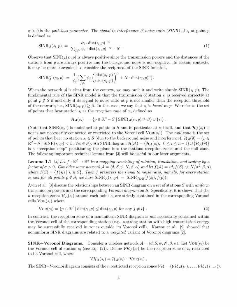
In this paper, we explore the behavior of the reception zones of SINR diagrams when restrictedto Voronoi diagrams. The resulting diagram, referred to as SINR+Voronoi diagram, consistsof n reception zones, one per station, obtained by the intersection of the SINR reception zoneswith their corresponding Voronoi cells. Studying SINR+Voronoi diagrams is motivated by thecomplexity of general nonuniform SINR zones and, perhaps more importantly, by the abundantusage of hexagonal networks in practice; cellular networks are commonly designed as hexagonalnetworks, where each node serves as a base-station to which mobile users must connect. A mobileuser is normally connected to the nearest base-station, hence each base-station serves all users thatare located inside its hexagonal grid cell (which is in fact its Voronoi cell). Due to the disk shape ofthe sensing range of the sensor devices, using a hexagonal tessellation topology is the most efficientway to cover the whole sensing area, and indeed many routing, location management and channelassignment protocols are based on it [6, 12, 13, 14, 15].It is thus intriguing to ask whether the reception zones of nonuniform SINR diagrams enjoy somedesirable properties (e.g., assume a convenient form) when restricted to their corresponding Voronoicells.

1

𝑠0

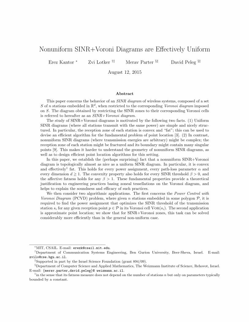
Figure 1: The overlay of an SINR diagram of a nonuniform wireless network on the correspondingVoronoi diagram. (a) Hexagonal Voronoi cells; the intersection between the reception region of stations0 and the Voronoi cell around it is highlighted in bold. (b) Slight random perturbation to a hexagonalnetwork. (c) Random positions.

In this paper, it is shown that while in general the reception zones in the nonuniform settingmight be fractured and their boundaries might contain many singular points, the restriction of areception zone to its Voronoi cell (e.g., hexagonal cell in the grid) behaves almost as nice as uniformzones: it is convex, and its fatness measure depends only on parameters typically bounded by aconstant, and in particular is independent of the number of stations in the network.

For an illustration see the reception zone of station s0 in Figure 1(a). These fundamentalproperties provide a theoretical justification to engineering practices basing regional tessellationson the Voronoi diagram, and helps to explain the soundness and efficacy of such practices.

To prove convexity, we extend the proof for the uniform setting of [3] to the nonuniform setting2.Apart from the theoretical interest, this result is of considerable practical significance, as obviously,having a convex reception zone inside each hexagonal cell may ease the development of protocolsfor various design and communication tasks such as scheduling, topology control and connectivity.We note that convexity within a Voronoi cell is important also in the mobile setting where no fixedtessellation can be assumed. For example, in the setting of Vehicular ad-hoc network (VANET)[17], the stations are mobile but each user is still mapped to the closest base-station. Hence,although the hexagonal tessellation is no longer preserved, the convexity within the (dynamic)Voronoi tessellation is still relevant (for an illustration, see Fig. 1(b)-(c)).

As an application for the convexity property, we consider the problem where one wishes to coverthe entire area of a given bounded polygon P by using a base-station network embedded in P. Onenatural way to do that is by assigning each base-station an area of coverage. Usually the base-station needs to cover the area of its Voronoi cell up to where it intersects with P. Assuming thepower with which each base-station transmits can be controlled, it is desirable to increase the SINRratio as much as possible in order to increase the capacity of the cellular network. The problemof determining the transmission energy of each base-station so as to maximize the capacity of theentire network is called the Power Control Voronoi Diagram (PCVD) problem. We show thatalthough PCVD is a non-convex and non-discrete problem, it can be solved in a nearly optimalmanner.

Our algorithm is especially useful in the mobile setting where the positions of base-stations vary

2Note that in the uniform setting too, convexity is guaranteed only inside the Voronoi cell, but since the entirereception zone is restricted to the Voronoi cell, this implies that the entire zone is convex. In contrast, in thenonuniform setting, the reception zone of a station with a high transmission energy might exceed its Voronoi cell.

2

with time. This scenario can happen in sudden-onset disasters and ad-hoc vehicle networks, sincein these cases, the network structure is not fixed and it is not clear how to divide the coverageareas between the base-stations. Although it is natural to use the Voronoi diagram, it is notclear how to assign the transmission energies in a way that guarantees a full coverage of the area ofinterest. The solution proposed in this paper for this problem has the advantage that it can adaptedto a dynamic setting quite efficiently since it depends upon the Voronoi tessellation that can bemaintained efficiently in a dynamic setting [8, 5]. By exploiting the convexity property in Voronoicells, we propose a discrete equivalent formulation of the PCVD problem. Specifically, thanks tothe convexity guarantee, we show that it is sufficient to insist on achieving the optimal thresholdβ only on the vertex set of each Voronoi cell (where unbounded Voronoi cells are bounded byusing a bounding polygon P that contains the entire coverage area). Computing power assignmentfor maximizing the coverage within Voronoi cells has been considered also in [16] from the gametheoretic point of view; yet no analytic result has been known so far for this problem.

We then turn to consider the fatness property. In [9], it was shown that the fatness of nonuniformzone can be bounded by some function of the maximum transmission power ψmax, the ambientnoise N , the SINR threshold β, the path-loss exponent α, the distance κ to the closest interferingstation and the number of stations in the network. The SINR+Voronoi zones are shown to havea fatness bound that is independent of n. In particular, since the network parameters α, β, κ,Nand ψmax are bounded in practice (i.e., unlike the number of stations), the SINR+Voronoi zonesare effectively fat. Finally, using [4], the convexity and the improved fatness bound imply anefficient approximate point location scheme for SINR+Voronoi zones whose preprocessing time andmemory requirements are significantly more efficient than those obtained in [9]. For a recent workon batched point location tasks, see recent work of [1].

1.2 Geometric notions and wireless networks

Geometric notions. We consider the d-dimensional Euclidean space Rd (for d ∈ Z≥1). Thedistance between points p and point q is denoted by dist(p, q) = ‖q− p‖. Denote the ball of radiusr centered at point p ∈ Rd by Bd(p, r) = {q ∈ Rd | dist(p, q) ≤ r}. Unless stated otherwise, weassume the 2-dimensional Euclidean plane, and omit d. The basic notions of open, closed, bounded,compact and connected sets of points are defined in the standard manner.

We use the term zone to describe a point set with some “niceness” properties. Unless statedotherwise, a zone refers to the union of an open connected set and some subset of its boundary. Itmay also refer to a single point or to the finite union of zones.

The point set P is said to be star-shaped with respect to point p ∈ P if the line segment p q iscontained in P for every point q ∈ P . In addition, P is said to be convex if it is star-shaped withrespect to any point p ∈ P , see [7].

For a bounded zone Z 6= ∅ and an internal p ∈ Z, denote the maximal and minimal diametersof Z w.r.t. p by δ(p, Z) = sup{r > 0 | Z ⊇ B(p, r)} and ∆(p, Z) = inf{r > 0 | Z ⊆ B(p, r)}, anddefine the fatness parameter of Z with respect to p to be ϕ(p, Z) = ∆(p, Z)/δ(p, Z). The zone Z issaid to be fat with respect to p if ϕ(p, Z) is bounded by some constant.

Wireless networks and SINR Diagrams. We consider a wireless networkA = 〈d, S, ψ,N , β, α〉,where d ∈ Z≥1 is the dimension, S = {s0, s1, . . . , sn−1} is a set of transmitting n ≥ 2 radio stationsembedded in the d-dimensional space, ψ is an assignment of a positive real transmitting power ψito each station si, N ≥ 0 is the background noise, β ≥ 0 is a constant reception threshold, and

3

α > 0 is the path-loss parameter. The signal to interference & noise ratio (SINR) of si at point pis defined as

SINRA(si, p) =ψi · dist(si, p)

−α∑j 6=i ψj · dist(sj , p)−α + N

. (1)

Observe that SINRA(si, p) is always positive since the transmission powers and the distances of thestations from p are always positive and the background noise is non-negative. In certain contexts,it may be more convenient to consider the reciprocal of the SINR function,

SINR−1A (si, p) =1

ψi

(∑j 6=i

ψj

(dist(si, p)

dist(sj , p)

)α+ N · dist(si, p)

α).

When the network A is clear from the context, we may omit it and write simply SINR(si, p). Thefundamental rule of the SINR model is that the transmission of station si is received correctly atpoint p /∈ S if and only if its signal to noise ratio at p is not smaller than the reception thresholdof the network, i.e., SINR(si, p) ≥ β. In this case, we say that si is heard at p. We refer to the setof points that hear station si as the reception zone of si, defined as

HA(si) = {p ∈ Rd − S | SINRA(si, p) ≥ β} ∪ {si} .

(Note that SINR(si, ·) is undefined at points in S and in particular at si itself, and that HA(si) isnot is not necessarily connected or restricted to the Voroni cell Vor(si)). The null zone is the setof points that hear no station si ∈ S (due to the background noise and interference), HA(∅) = {p ∈Rd−S | SINR(si, p) < β, ∀si ∈ S}. An SINR diagram H(A) = {HA(si), 0 ≤ i ≤ n−1}∪{HA(∅)}is a “reception map” partitioning the plane into the stations reception zones and the null zone.The following important technical lemma from [3] will be useful in our later arguments.

Lemma 1.1 [3] Let f : Rd → Rd be a mapping consisting of rotation, translation, and scaling by afactor of σ > 0. Consider some network A = 〈d, S, ψ,N , β, α〉 and let f(A) = 〈d, f(S), ψ,N /σ2, β, α〉,where f(S) = {f(si) | si ∈ S}. Then f preserves the signal to noise ratio, namely, for every stationsi and for all points p /∈ S, we have SINRA(si, p) = SINRf(A)(f(si), f(p)).

Avin et al. [3] discuss the relationships between an SINR diagram on a set of stations S with uniformtransmission powers and the corresponding Voronoi diagram on S. Specifically, it is shown that then reception zones HA(si) around each point si are strictly contained in the corresponding Voronoicells Vor(si) where

Vor(si) = {p ∈ Rd | dist(si, p) ≤ dist(sj , p) for any j 6= i} . (2)

In contrast, the reception zone of a nonuniform SINR diagram is not necessarily contained withinthe Voronoi cell of the corresponding station (e.g., a strong station with high transmission energymay be successfully received in zones outside its Voronoi cell). Kantor et al. [9] showed thatnonuniform SINR diagrams are related to a weighted variant of Voronoi diagrams [2].

SINR+Voronoi Diagrams. Consider a wireless network A = 〈d, S, ψ,N , β, α〉. Let Vor(si) bethe Voronoi cell of station si (see Eq. (2)). Define VHA(si) be the reception zone of si restrictedto its Voronoi cell, where

VHA(si) = HA(si) ∩Vor(si) .

The SINR+Voronoi diagram consists of the n restricted reception zones VH = 〈VHA(s0), . . . ,VHA(sn−1)〉.

4

2 Convexity of SINR+Voronoi Zones

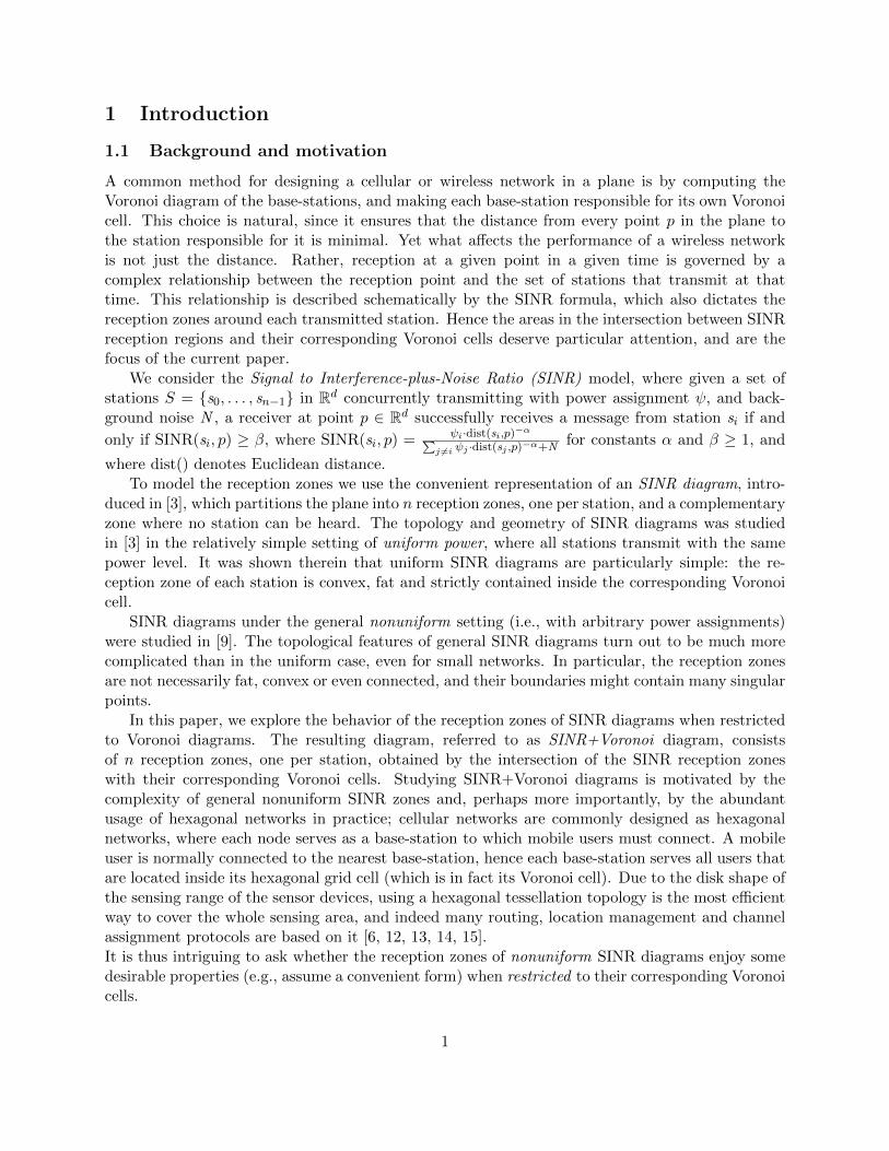
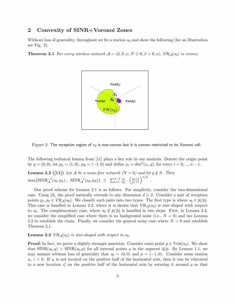
Without loss of generality, throughout we fix a station s0 and show the following (for an illustrationsee Fig. 2).

Theorem 2.1 For every wireless network A = 〈d, S, ψ,N ≥ 0, β > 0, α〉, VHA(s0) is convex.

𝑉ℋ(𝑠0)

Figure 2: The reception region of s2 is non-convex but it is convex restricted to its Voronoi cell.

The following technical lemma from [11] plays a key role in our analysis. Denote the origin pointby q = (0, 0), let pL = (1, 0), pR = (−1, 0) and define ρi = dist2(si, q), for every i = 0, ..., n− 1.

Lemma 2.2 ([11]) Let A be a noise-free network (N = 0) and let q /∈ S. Then

max{SINR−1A (s0, pL) , SINR−1A (s0, pR)} ≥∑n−1

i=1ψiψ0·(ρ0+1ρi+1

)α/2.

Our proof scheme for Lemma 2.1 is as follows. For simplicity, consider the two-dimensionalcase. Using [3], the proof naturally extends to any dimension d ≥ 2. Consider a pair of receptionpoints p1, p2 ∈ VHA(s0). We classify such pairs into two types. The first type is where s0 ∈ p1 p2.This case is handled in Lemma 2.3, where it is shown that VHA(s0) is star-shaped with respectto s0. The complementary case, where s0 6∈ p1 p2 is handled in two steps. First, in Lemma 2.4,we consider the simplified case where there is no background noise (i.e., N = 0) and use Lemma2.2 to establish the claim. Finally, we consider the general noisy case where N > 0 and establishTheorem 2.1.

Lemma 2.3 VHA(s0) is star-shaped with respect to s0.

Proof: In fact, we prove a slightly stronger assertion. Consider some point p ∈ Vor(s0). We showthat SINR(s0, q) > SINR(s0, p) for all internal points q in the segment s0 p. By Lemma 1.1, wemay assume without loss of generality that s0 = (0, 0) and p = (−1, 0). Consider some stationsi, i > 0. If si is not located on the positive half of the horizontal axis, then it can be relocatedto a new location s ′i on the positive half of the horizontal axis by rotating it around p so that

5

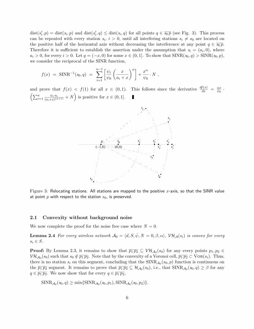
dist(s ′i, p) = dist(si, p) and dist(s ′i, q) ≤ dist(si, q) for all points q ∈ s0 p (see Fig. 3). This processcan be repeated with every station si, i > 0, until all interfering stations si 6= s0 are located onthe positive half of the horizontal axis without decreasing the interference at any point q ∈ s0 p.Therefore it is sufficient to establish the assertion under the assumption that si = (ai, 0), whereai > 0, for every i > 0. Let q = (−x, 0) for some x ∈ (0, 1]. To show that SINR(s0, q) > SINR(s0, p),we consider the reciprocal of the SINR function,

f(x) = SINR−1(s0, q) =n−1∑i=1

[ψiψ0

(x

ai + x

)α]+xα

ψ0·N ,

and prove that f(x) < f(1) for all x ∈ (0, 1). This follows since the derivative df(x)dx = αx

ψ0·(∑n

i=1ψi·ai

(ai+x)(α+1) + N)

is positive for x ∈ (0, 1].

Figure 3: Relocating stations. All stations are mapped to the positive x-axis, so that the SINR valueat point p with respect to the station s0, is preserved.

2.1 Convexity without background noise

We now complete the proof for the noise free case where N = 0.

Lemma 2.4 For every wireless network A0 = 〈d, S, ψ,N = 0, β, α〉, VHA(si) is convex for everysi ∈ S.

Proof: By Lemma 2.3, it remains to show that p1 p2 ⊆ VHA0(s0) for any every points p1, p2 ∈VHA0(s0) such that s0 /∈ p1 p2. Note that by the convexity of a Voronoi cell, p1 p2 ⊂ Vor(si). Thus,there is no station si on this segment, concluding that the SINRA0(s0, p) function is continuous onthe p1 p2 segment. It remains to prove that p1 p2 ⊆ HA0(s0), i.e., that SINRA0(s0, q) ≥ β for anyq ∈ p1 p2. We now show that for every q ∈ p1 p2,

SINRA0(s0, q) ≥ min{SINRA0(s0, p1), SINRA0(s0, p2)}.

6

Specifically, we show that the dual statement holds, namely, that

SINR−1A0(s0, q) ≤ max

{SINR−1A0

(s0, p1),SINR−1A0(s0, p2)

}. (3)

By Lemma 1.1 and by the continuity of the SINRA function in the segment p1 p2, it is sufficientto consider the case where p1 = (−1, 0), p2 = (1, 0) and q = (0, 0), the middle point between p1and p2 on the segment. By applying Lemma 2.2, we have

max{SINR−1A0(s0, p1) , SINR−1A0

(s0, p2)} ≥n−1∑i=1

ψiψ0·(ρ0 + 1

ρi + 1

)α/2. (4)

On the other hand, by Eq. (2),

SINR−1A0(s0, q) =

n−1∑i=1

ψiψ0·(ρ0ρi

)α/2. (5)

As q ∈ Vor(s0), we have that ρi > ρ0 and hence ρ0/ρi < (ρ0+1)/(ρi+1) for every i ∈ {1, ..., n−1}.This, together with Eq. (4) and (5), implies Ineq. (3).

2.2 Convexity with background noise

We now consider the general case where N ≥ 0.Proof: [Theorem 2.1] Consider two points p1, p2 ∈ VHA(s0). We need to show that p1 p2 ⊆VHA(s0). By Lemma 1.1, we may assume without loss of generality that p1 = (−1, 0) and p2 =(1, 0). Let dN = max{dist(s0, p1),dist(s0, p2)}.

Let A∗ be a noise-free (n + 1)-station network obtained from A by replacing the backgroundnoise with a new station sN located in (0, dN ) with transmission power ψN = N · (d2N +1)α/2. Thatis, A∗ = 〈d = 2, S∗, ψ∗,N = 0, β, α〉, where S∗ = S ∪ {sN} and ψ∗ = (ψ0, ..., ψn−1, ψN ). It is easyto verify that ψN · dist(sN , pi)

−α = N and ψN · dist(sN , q)−α ≥ N , for every q ∈ p1 p2. Thus, on

the one hand,

SINRA∗(s0, pi) = SINRA(s0, pi), for i ∈ {1, 2}, (6)

and on the other hand, for all points q ∈ p1 p2,

SINRA(s0, q) ≥ SINRA∗(s0, q). (7)

We now show that p1, p2 ∈ VHA∗(s0). We first claim that p1, p2 ∈ Vor∗(s0) where Vor∗ is theVoronoi diagram of the set S∗. Since p1, p2 ∈ VHA(s0), in particular p1, p2 ∈ Vor(s0). Thisimplies that dist(s0, pi) ≤ dist(sj , pi), for every i ∈ {1, 2} and j ∈ {1, ..., n − 1}. In addition,dist(sN , pi) > dN ≥ dist(s0, pi), implying that p1, p2 ∈ Vor∗(s0) as needed. It remains to showthat p1, p2 ∈ HA∗(s0). Since p1, p2 ∈ HA(s0), SINRA(s0, pi) ≥ β for i ∈ {1, 2}. Thus, by Eq. (6),SINRA∗(s0, pi) ≥ β as well, and p1, p2 ∈ HA∗(s0). Finally, since p1, p2 ∈ VHA∗(s0) where A∗ is anoise free network, by Lemma 2.4 it holds that SINRA∗(s0, q) ≥ β, for all points q ∈ p1 p2. Thus,by Ineq. (7), also SINRA(s0, q) ≥ β, for all points q ∈ p1 p2, are required. The lemma follows.

Theorem 2.1 is established.

7

3 Fatness of SINR+Voronoi Zones

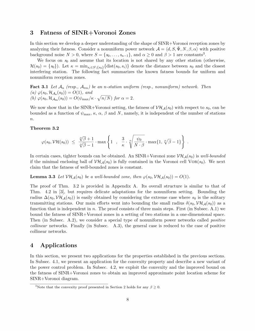
In this section we develop a deeper understanding of the shape of SINR+Voronoi reception zones byanalyzing their fatness. Consider a nonuniform power network A = 〈d, S, Ψ,N , β, α〉 with positivebackground noise N > 0, where S = {s0, . . . , sn−1}, and α ≥ 0 and β > 1 are constants3.

We focus on s0 and assume that its location is not shared by any other station (otherwise,H(s0) = {s0}). Let κ = minsi∈S\{s0}{dist(s0, si)} denote the distance between s0 and the closestinterfering station. The following fact summarizes the known fatness bounds for uniform andnonuniform reception zones.

Fact 3.1 Let Au (resp., Anu) be an n-station uniform (resp., nonuniform) network. Then(a) ϕ(s0,HAu(s0)) = O(1), and(b) ϕ(s0,HAnu(s0)) = O(ψmax/κ ·

√n/N ) for α = 2.

We now show that in the SINR+Voronoi setting, the fatness of VHA(s0) with respect to s0, can bebounded as a function of ψmax, κ, α, β and N , namely, it is independent of the number of stationsn.

Theorem 3.2

ϕ(s0,VH(s0)) ≤α√β + 1

α√β − 1

·max

{1 ,

3

κ· α√

ψ0

N · β·max{1, α

√β − 1}

}.

In certain cases, tighter bounds can be obtained. An SINR+Voronoi zone VHA(s0) is well-boundedif the minimal enclosing ball of VHA(s0) is fully contained in the Voronoi cell Vor(s0). We nextclaim that the fatness of well-bounded zones is constant.

Lemma 3.3 Let VHA(s0) be a well-bounded zone, then ϕ(s0,VHA(s0)) = O(1).

The proof of Thm. 3.2 is provided in Appendix A. Its overall structure is similar to that ofThm. 4.2 in [3], but requires delicate adaptations for the nonuniform setting. Bounding theradius ∆(s0,VHA(s0)) is easily obtained by considering the extreme case where s0 is the solitarytransmitting stations. Our main efforts went into bounding the small radius δ(s0,VHA(s0)) as afunction that is independent in n. The proof consists of three main steps. First (in Subsec. A.1) webound the fatness of SINR+Voronoi zones in a setting of two stations in a one-dimensional space.Then (in Subsec. A.2), we consider a special type of nonuniform power networks called positivecollinear networks. Finally (in Subsec. A.3), the general case is reduced to the case of positivecollinear networks.

4 Applications

In this section, we present two applications for the properties established in the previous sections.In Subsec. 4.1, we present an application for the convexity property and describe a new variant ofthe power control problem. In Subsec. 4.2, we exploit the convexity and the improved bound onthe fatness of SINR+Voronoi zones to obtain an improved approximate point location scheme forSINR+Voronoi diagram.

3Note that the convexity proof presented in Section 2 holds for any β ≥ 0.

8

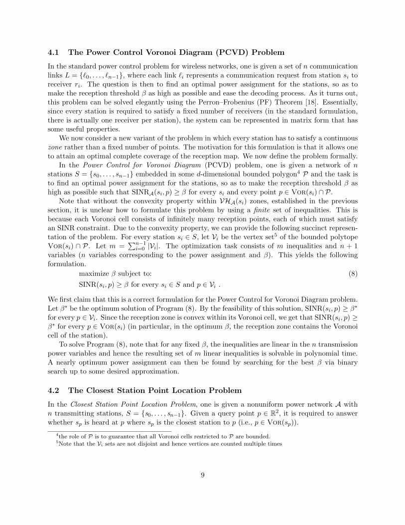
4.1 The Power Control Voronoi Diagram (PCVD) Problem

In the standard power control problem for wireless networks, one is given a set of n communicationlinks L = {`0, . . . , `n−1}, where each link `i represents a communication request from station si toreceiver ri. The question is then to find an optimal power assignment for the stations, so as tomake the reception threshold β as high as possible and ease the decoding process. As it turns out,this problem can be solved elegantly using the Perron–Frobenius (PF) Theorem [18]. Essentially,since every station is required to satisfy a fixed number of receivers (in the standard formulation,there is actually one receiver per station), the system can be represented in matrix form that hassome useful properties.

We now consider a new variant of the problem in which every station has to satisfy a continuouszone rather than a fixed number of points. The motivation for this formulation is that it allows oneto attain an optimal complete coverage of the reception map. We now define the problem formally.

In the Power Control for Voronoi Diagram (PCVD) problem, one is given a network of nstations S = {s0, . . . , sn−1} embedded in some d-dimensional bounded polygon4 P and the task isto find an optimal power assignment for the stations, so as to make the reception threshold β ashigh as possible such that SINRA(si, p) ≥ β for every si and every point p ∈ Vor(si) ∩ P.

Note that without the convexity property within VHA(si) zones, established in the previoussection, it is unclear how to formulate this problem by using a finite set of inequalities. This isbecause each Voronoi cell consists of infinitely many reception points, each of which must satisfyan SINR constraint. Due to the convexity property, we can provide the following succinct represen-tation of the problem. For every station si ∈ S, let Vi be the vertex set5 of the bounded polytopeVor(si) ∩ P. Let m =

∑n−1i=0 |Vi|. The optimization task consists of m inequalities and n + 1

variables (n variables corresponding to the power assignment and β). This yields the followingformulation.

maximize β subject to: (8)

SINR(si, p) ≥ β for every si ∈ S and p ∈ Vi .

We first claim that this is a correct formulation for the Power Control for Voronoi Diagram problem.Let β∗ be the optimum solution of Program (8). By the feasibility of this solution, SINR(si, p) ≥ β∗for every p ∈ Vi. Since the reception zone is convex within its Voronoi cell, we get that SINR(si, p) ≥β∗ for every p ∈ Vor(si) (in particular, in the optimum β, the reception zone contains the Voronoicell of the station).

To solve Program (8), note that for any fixed β, the inequalities are linear in the n transmissionpower variables and hence the resulting set of m linear inequalities is solvable in polynomial time.A nearly optimum power assignment can then be found by searching for the best β via binarysearch up to some desired approximation.

4.2 The Closest Station Point Location Problem

In the Closest Station Point Location Problem, one is given a nonuniform power network A withn transmitting stations, S = {s0, . . . , sn−1}. Given a query point p ∈ R2, it is required to answerwhether sp is heard at p where sp is the closest station to p (i.e., p ∈ Vor(sp)).

4the role of P is to guarantee that all Voronoi cells restricted to P are bounded.5Note that the Vi sets are not disjoint and hence vertices are counted multiple times

9

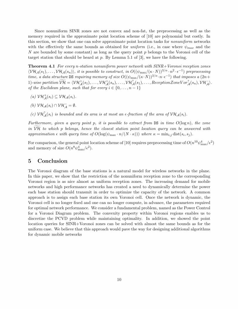
Since nonuniform SINR zones are not convex and non-fat, the preprocessing as well as thememory required in the approximate point location scheme of [10] are polynomial but costly. Inthis section, we show that one can solve approximate point location tasks for nonuniform networkswith the effectively the same bounds as obtained for uniform (i.e., in case where ψmax and theN are bounded by some constant) as long as the query point p belongs to the Voronoi cell of thetarget station that should be heard at p. By Lemma 5.1 of [3], we have the following.

Theorem 4.1 For every n-station nonuniform power network with SINR+Voronoi reception zones〈VHA(s1), . . . ,VHA(sn)〉, it is possible to construct, in O((ψmax/(κ ·N ))3/α ·n2 · ε−1) preprocessingtime, a data structure DS requiring memory of size O((ψmax/(κ·N ))3/α ·n·ε−1) that imposes a (2n+

1)-wise partition VH = 〈VH+A(s1), . . . ,VH+

A(sn), . . . ,VH?A(s1), . . . , ReceptionZoneV or

?A(sn),VH−A〉.

of the Euclidean plane, such that for every i ∈ {0, . . . , n− 1}

(a) VH+A(si) ⊆ VHA(si).

(b) VHA(si) ∩ VH−A = ∅.

(c) VH?A(si) is bounded and its area is at most an ε-fraction of the area of VHA(si).

Furthermore, given a query point p, it is possible to extract from DS in time O(log n), the zone

in VH to which p belongs, hence the closest station point location query can be answered withapproximation ε with query time of O(log(ψmax · n/(N · κ))) where κ = mini,j dist(si, sj).

For comparison, the general point location scheme of [10] requires preprocessing time ofO(n10ψ4max/ε

2)and memory of size O(n8ψ4

max/ε2).

5 Conclusion

The Voronoi diagram of the base stations is a natural model for wireless networks in the plane.In this paper, we show that the restriction of the nonuniform reception zone to the correspondingVoronoi region is as nice almost as uniform reception zones. The increasing demand for mobilenetworks and high performance networks has created a need to dynamically determine the powereach base station should transmit in order to optimize the capacity of the network. A commonapproach is to assign each base station its own Voronoi cell. Once the network is dynamic, theVoronoi cell is no longer fixed and one can no longer compute, in advance, the parameters requiredfor optimal network performance. We consider a fundamental problem, named as the Power Controlfor a Voronoi Diagram problem. The convexity property within Voronoi regions enables us todiscretize the PCVD problem while maintaining optimality. In addition, we showed the pointlocation queries for SINR+Voronoi zones can be solved with almost the same bounds as for theuniform case. We believe that this approach would pave the way for designing additional algorithmsfor dynamic mobile networks

10

References

[1] B. Aronov and M.J. Katz. Batched point location in SINR diagrams via algebraic tools. In ICALP,2015.

[2] F. Aurenhammer and H. Edelsbrunner. An optimal algorithm for constructing the weighted voronoidiagram in the plane. Pattern Recognition, 17, 1984.

[3] C. Avin, Y. Emek, E. Kantor, Z. Lotker, D. Peleg, and L. Roditty. SINR diagrams: Convexity and itsapplications in wireless networks. J. ACM, 59(4), 2012.

[4] C. Avin, Z. Lotker, and Y.-A. Pignolet. On the power of uniform power: Capacity of wireless networkswith bounded resources. In Proc. of ESA, pages 373–384, 2009.

[5] J. Basch, L.J. Guibas, and J. Hershberger. Data structures for mobile data, 1997.

[6] B. Chen, K. Jamieson, H. Balakrishnan, and R. Morris. Span: An energy-efficient coordination algo-rithm for topology maintenance in ad hoc wireless networks. Wireless Networks, 8:481–494, 2002.

[7] M. de Berg, O. Cheong, M. van Kreveld, and M. Overmars. Computational Geometry: Algorithms andApplications. Springer-Verlag, 2008.

[8] L.J. Guibas, J.S.B Mitchell, and T. Roos. Voronoi diagrams of moving points in the plane. In Proc. ofWG. SV, 1992.

[9] E. Kantor, Z. Lotker, M. Parter, and D. Peleg. The topology of wireless communication. In Proc.STOC, 2011.

[10] E. Kantor, Z. Lotker, M. Parter, and D. Peleg. The topology of wireless communication. Inhttp://arxiv.org/pdf/1103.4566v2.pdf, 2011.

[11] E. Kantor, Z. Lotker, M. Parter, and D. Peleg. The minimum principle of SINR and applications.Submitted, 2015.

[12] Y. Kim, J. Kim, H. Nam, and S. An. Hex-grid based routing protocol in wireless sensor networks. InComputat. Sci. & Eng., pages 683–688, 2012.

[13] F. G. Nocetti, I. Stojmenovic, and J. Zhang. Addressing and routing in hexagonal networks withapplications for tracking mobile users and connection rerouting in cellular networks. IEEE Trans. Par.& Distr. Syst., 13:963–971, 2002.

[14] L.R. Ping, G. Rogers, S. Zhou, and J. Zic. Topology control with hexagonal tessellation. 2:91–98, 2007.

[15] I. Stojmenovic. Honeycomb networks: Topological properties and communication algorithms. IEEETrans. Par. & Distr. Syst., 8:1036–1042, 1997.

[16] X. Xu, Y. Li, R. Gao, and X. Tao. Joint voronoi diagram and game theory-based power control schemefor the hetnet small cell networks. EURASIP J. Wireless Comm. and Networking, 2014:213, 2014.

[17] S. Yousefi, M. S. Mousavi, and M. Fathy. Vehicular adhoc networks (vanets): challenges and perspec-tives. In IEEE ITS Telecomm., pages 761–766, 2006.

[18] J. Zander. Performance of optimum transmitter power control in cellular radiosystems. IEEE Tr. Vehic.Technol., 41:57–62, 1992.

0 1

s s1

µ µrl

0

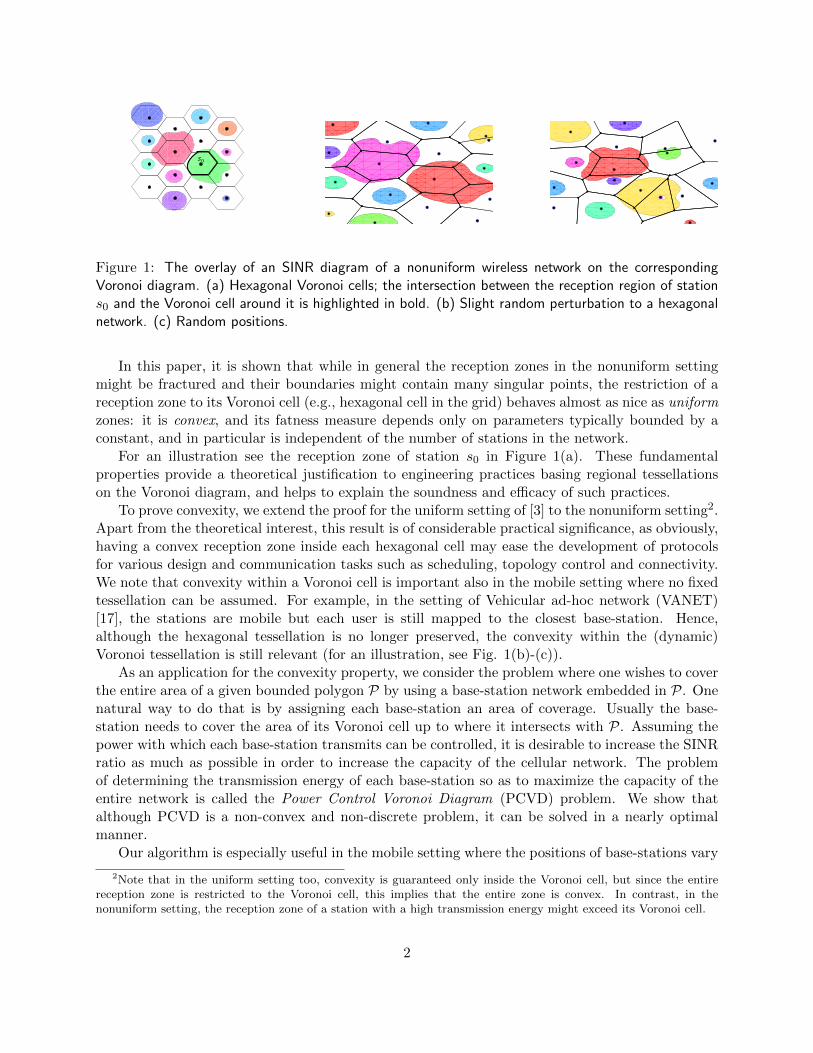
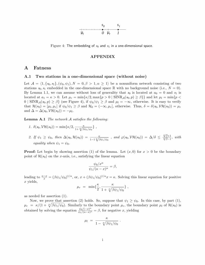
Figure 4: The embedding of s0 and s1 in a one-dimensional space.

APPENDIX

A Fatness

A.1 Two stations in a one-dimensional space (without noise)

Let A = 〈1, {s0, s1}, (ψ0, ψ1),N = 0, β > 1, α ≥ 1〉 be a nonuniform network consisting of twostations s0, s1 embedded in the one-dimensional space R with no background noise (i.e., N = 0).By Lemma 1.1, we can assume without loss of generality that s0 is located at a0 = 0 and s1 islocated at a1 = κ > 0. Let µr = min{κ/2,max{p > 0 | SINRA(s0, p) ≥ β}} and let µl = min{p <0 | SINRA(s0, p) ≥ β} (see Figure 4), if ψ0/ψ1 ≥ β and µl = −∞, otherwise. It is easy to verifythat H(s0) = [µl, µr] if ψ0/ψ1 ≥ β and H0 = (−∞, µr], otherwise. Thus, δ = δ(s0,VH(s0)) = µrand ∆ = ∆(s0,VH(s0)) = −µl.

Lemma A.1 The network A satisfies the following:

1. δ(s0,VH(s0)) = min{κ/2, κ

1+ α√βψ1/ψ0

} ,

2. If ψ1 ≥ ψ0, then ∆(s0,H(s0)) = κ

1−1 α√βψ1/ψ0

, and ϕ(s0,VH(s0)) = ∆/δ ≤α√β+1α√β−1 , with

equality when ψ1 = ψ0.

Proof: Let begin by showing assertion (1) of the lemma. Let (x, 0) for x > 0 be the boundarypoint of H(s0) on the x-axis, i.e., satisfying the linear equation

ψ0/xα

ψ1/(κ− x)α= β,

leading to κ−xx = (βψ1/ψ0)

1/α, or, x+ (βψ1/ψ0)1/αx = κ. Solving this linear equation for positive

x yields,

µr = min{κ2,

κ

1 + α√βψ1/ψ0

} ,

as needed for assertion (1).Now, we prove that assertion (2) holds. So, suppose that ψ1 ≥ ψ0. In this case, by part (1),

µr = κ/(1 + α√βψ1/ψ0). Similarly to the boundary point µr, the boundary point µl of H(s0) is

obtained by solving the equation ψ0/(−x)αψ1/(κ−x)α = β, for negative x, yielding

µl =κ

1− α√βψ1/ψ0

.

i

0s1 s2 s3 s4

1a a2 a3 a40

µ µl

s

r

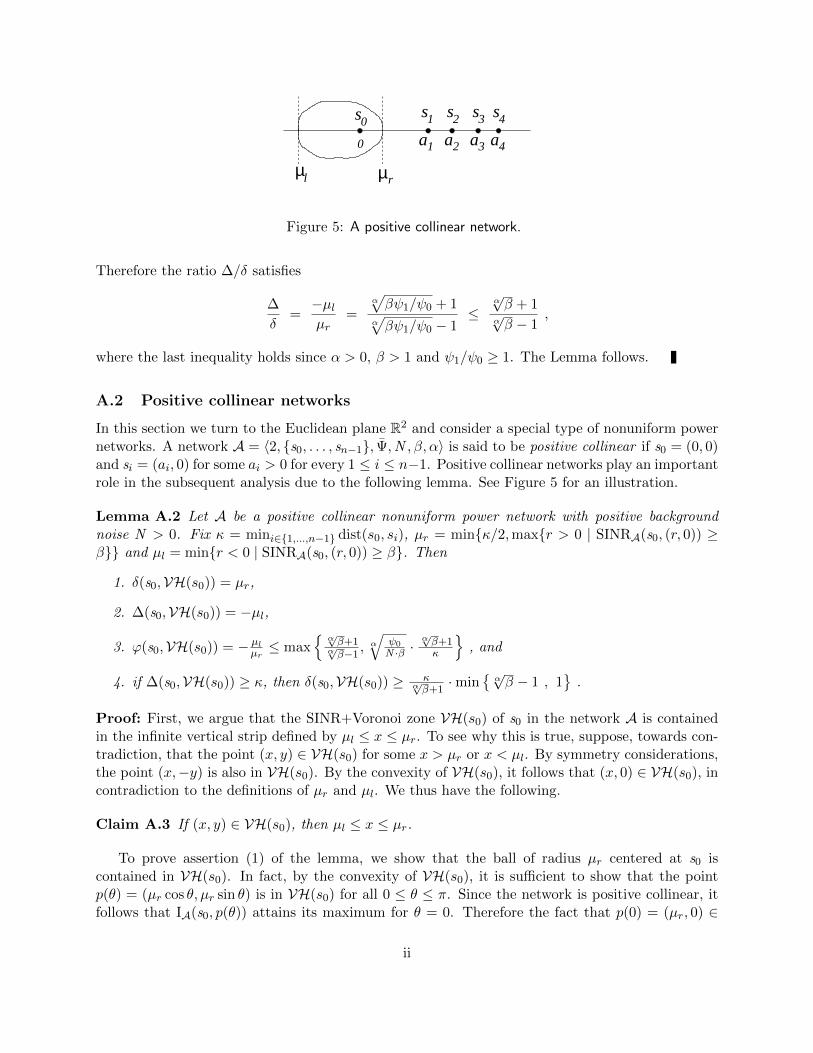
Figure 5: A positive collinear network.

Therefore the ratio ∆/δ satisfies

∆

δ=−µlµr

=α√βψ1/ψ0 + 1

α√βψ1/ψ0 − 1

≤α√β + 1

α√β − 1

,

where the last inequality holds since α > 0, β > 1 and ψ1/ψ0 ≥ 1. The Lemma follows.

A.2 Positive collinear networks

In this section we turn to the Euclidean plane R2 and consider a special type of nonuniform powernetworks. A network A = 〈2, {s0, . . . , sn−1}, Ψ,N , β, α〉 is said to be positive collinear if s0 = (0, 0)and si = (ai, 0) for some ai > 0 for every 1 ≤ i ≤ n−1. Positive collinear networks play an importantrole in the subsequent analysis due to the following lemma. See Figure 5 for an illustration.

Lemma A.2 Let A be a positive collinear nonuniform power network with positive backgroundnoise N > 0. Fix κ = mini∈{1,...,n−1} dist(s0, si), µr = min{κ/2,max{r > 0 | SINRA(s0, (r, 0)) ≥β}} and µl = min{r < 0 | SINRA(s0, (r, 0)) ≥ β}. Then

1. δ(s0,VH(s0)) = µr,

2. ∆(s0,VH(s0)) = −µl,

3. ϕ(s0,VH(s0)) = − µlµr≤ max

{α√β+1α√β−1 ,

α

√ψ0

N ·β ·α√β+1κ

}, and

4. if ∆(s0,VH(s0)) ≥ κ, then δ(s0,VH(s0)) ≥ κα√β+1

·min{α√β − 1 , 1

}.

Proof: First, we argue that the SINR+Voronoi zone VH(s0) of s0 in the network A is containedin the infinite vertical strip defined by µl ≤ x ≤ µr. To see why this is true, suppose, towards con-tradiction, that the point (x, y) ∈ VH(s0) for some x > µr or x < µl. By symmetry considerations,the point (x,−y) is also in VH(s0). By the convexity of VH(s0), it follows that (x, 0) ∈ VH(s0), incontradiction to the definitions of µr and µl. We thus have the following.

Claim A.3 If (x, y) ∈ VH(s0), then µl ≤ x ≤ µr.

To prove assertion (1) of the lemma, we show that the ball of radius µr centered at s0 iscontained in VH(s0). In fact, by the convexity of VH(s0), it is sufficient to show that the pointp(θ) = (µr cos θ, µr sin θ) is in VH(s0) for all 0 ≤ θ ≤ π. Since the network is positive collinear, itfollows that IA(s0, p(θ)) attains its maximum for θ = 0. Therefore the fact that p(0) = (µr, 0) ∈

ii

H(s0) implies that p(θ) ∈ VH(s0) for all 0 ≤ θ ≤ π as desired. Assertion (1) follows. Next, we showthat ∆ is realized by the point (µl, 0). Indeed, by the triangle inequality, all points at distance kfrom s0 are at distance at most k+ai from si = (ai, 0), with equality attained for the point (−k, 0).Thus the minimum interference to s0 under A among all points at distance k from s0 is attainedat the point (−k, 0). Therefore, by the definition of µl, there cannot exist any point p ∈ VH(s0)such that dist(p, s0) > −µl. Assertion (2) follows.

It remains to establish assertions (3) and (4). Recall that the leftmost station other than s0is located at (κ, 0). By definition, µr < κ/2. Denote the energy of station si at (µr, 0) by Ei =E(si, (µr, 0)) = ψi · (ai− µr)−α. We construct a new (n+ 1)-station network A′ = 〈2, S′, ψ′, 0, β, α〉consisting of s0 and n new stations s ′0, . . . , s

′n−1, all located at (κ, 0). We set the transmission power

ψ′i of the new stations s ′i to

ψ′i =

{Ei · (κ− µr)α for 1 ≤ i ≤ n− 1; andN · (κ− µr)α for i = n.

This ensures that the energy produced by these stations at (µr, 0) is

E(s ′i, (µr, 0)) =

{Ei for 1 ≤ i ≤ n− 1, andN for i = n.

Let ∆ = ∆(s0,VHA(s0)), ∆′ = ∆(s0,VHA′(s′0)). The small radii δ and δ′ are defined analogously.Note that the Voronoi cell of s0 is the same in both networks A and A′.

The network A′ falls into the setting of Subsec. A.1: the stations s ′1, . . . , s′n share the same

location, thus they can be considered as a single station s1 with transmission power ψ1 =∑n

i=1 ψ′i.

Define µ′r = min{κ/2,max{r > 0 | SINRA′(s0, (r, 0)) ≥ β}}

µ′l =

{min{r < 0 | SINRA′(s0, (r, 0)) ≥ β} if ψ1 ≥ βψ0

−∞ otherwise.

The restriction of the VHA′(s0) to the x-axis is thus [µ′l, µ′r]. In addition, it is easy to verify

that ∆′ ≤ α√ψ0/N · β (i.e., this is attained when only s0 transmits). By A.1, −µ′l/µ′r ≤

α√β+1α√β−1 , if

ψ1 ≥ ψ0 and δ′ ≤ κ1+ α√β otherwise.

The remaining of the proof relies on establishing the following two bounds.

(A1) SINRA′(s0, (r, 0)) ≤ SINRA(s0, (r, 0)) for all µr ≤ r < κ; and

(A2) SINRA′(s0, (r, 0)) ≥ SINRA(s0, (r, 0)) for all r ≤ µr, r 6= 0.

By combining bounds (A1) and (A2), we conclude that µ′r ≤ µr and µ′l ≤ µl . Thus, ∆′ ≥ ∆and δ′ ≤ δ. Assertion (3) of the lemma holds, by combining this together with the facts that (i)

∆/δ ≤ ∆′/δ′ ≤α√β+1α√β−1 , if ψ1 ≥ ψ0, and (ii) δ ≥ κ/(1 + α

√β) and ∆ ≤ ψ0/(β ·N ), otherwise.

For showing assertion (4), we consider two cases. If ψ1 < ψ0, then as mention above, we havethat δ ≥ δ′ ≥ κ

α√β+1as needed for assertion (4). Otherwise, suppose that ψ1 ≥ ψ0 and that

∆ ≥ κ (the second inequality is the condition of that assertion). Combining this with the factsthat ∆′ ≥ ∆, δ′ ≤ δ and with Assertion (2) of Lemma A.1,

κ/δ ≤ ∆/δ ≤ ∆′/δ′ ≤α√β + 1

α√β − 1

,

iii

which completes the proof of Assertion (4).To establish Inequalities (A1) and (A2), consider some point p = (r, 0), where r < κ, r 6= 0.

For every 1 ≤ i ≤ n− 1, we have

E(si, p) = ψi · (ai − r)−α , while E(s ′i, p) = ψ′i · (κ− r)−α =ψi · (κ− µr)α

(κ− r)α(ai − µr)α.

Comparing these two expressions, we get E(si, p) ≥ E(s ′i, p), or equivalently, (κ − r)(ai − µr) ≥(κ− µr)(ai − r). Rearranging, κai − κµr − air + rµr ≥ κai − κr − aiµr + rµr, or

µr(ai − κ) ≥ r(ai − κ) ,

Note that the inequality holds with equality if and only ai = κ, which, by definition, implies thatE(si, p) = E(s ′i, p). Therefore, the contribution of s ′i to the total interference at p = (0, r) is notlarger than that of si as long as r ≤ µr and not smaller than that of si as long as µr ≤ r < κ. Onthe other hand, the energy of s ′n at p = (r, 0) satisfies E(s ′n, p) ≤ N for all κ ≤ µr and E(s ′n, p) ≥ Nfor all µr ≤ r < κ. Inequalities (A1) and (A2) follow.

A.3 General uniform power networks in d-dimensional space

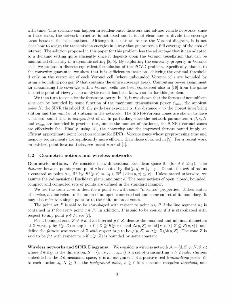
We are now ready to prove Thm. 3.2.Proof: [Proof of Theorem 3.2.] Consider an arbitrary nonuniform power network A = 〈d, S, Ψ,N >0, β, α〉, with positive noise, where S = {s0, . . . , sn−1} and β > 1 is a constant. We employLemma 1.1 to assume without loss of generality that s0 is located at (0, ..., 0) and that max{dist(s0, q

′) |q′ ∈ VHA(s0) is realized by a point q′ = (−∆, 0, ..., 0) on the negative x-axis. Let

q =

{(−∆, 0, ..., 0) if ∆ ≤ κ/3(−κ/3, 0, ..., 0).

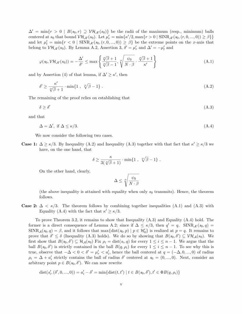
Note that by definition, q is an internal point in Vor(s0). By the convexity of the VHA(s0), itholds that q ∈ VHA(s0). We now construct a new positive collinear nonuniform power networkA′ = 〈d, {s0, s ′1, . . . , s ′n−1}, Ψ,N > 0, β, α〉, obtained from A by rotating each station si around thepoint q until it reaches the Euclidean plane at the positive x-axis (see Figure 6). More formally,the location of s0 remains unchanged and s ′i = (a′i, 0), where a′i = dist(si, q) − dist(s0, q) for every1 ≤ i ≤ n − 1. Note that, since q ∈ Vor(s0), it holds that dist(s0, q) < dist(si, q) (and hencea′i > 0), for every i = 1, ..., n − 1. Thus, A′ is a positive collinear network. In addition, for everyi = 1, ..., n− 1, the following three properties hold.(P1) dist(s ′i, q) = dist(si, q);(P2) dist(s′0, s

′i) ≤ dist(s0, si); and

(P3) dist(s′0, s′i) ≥ κ/3.

Property (P1) is trivially holds by the contraction of A′ in which the stations preserves the distancefrom q. Property (P2) holds, since dist(s′0, s

′i) = dist(si, q) − dist(s0, q), whereas dist(s0, si) ≥

dist(si, q)−dist(s0, q). Finally, Property (P3) holds, since (i) dist(s0, q) ≤ κ/3; (ii) dist(s0, si) ≥ κ,hence, (iii)dist(si, q) ≥ 2κ/3. Property (P3) holds, by combining together (ii), (iii) with (P1).

Let κ′ = mini∈{1,...,n−1} dist(s0, s′i) be the distance from s0 to the closest interfering station

in A′. By Property (P2), it follows that κ′ ≤ κ and by Property (P3) it follows that κ′ ≥ κ/3.We now consider the fatness of VHA′(s0). Let δ′ = max{r > 0 | B(s0, r) ⊆ VHA′(s0)} and

iv

∆′ = min{r > 0 | B(s0, r) ⊇ VHA′(s0)} be the radii of the maximum (resp., minimum) ballscentered at s0 that bound VHA′(s0). Let µ′r = min{κ′/2,max{r > 0 | SINRA′(s0, (r, 0, ..., 0)) ≥ β}}and let µ′l = min{r < 0 | SINRA′(s0, (r, 0, ..., 0)) ≥ β} be the extreme points on the x-axis thatbelong to VHA′(s0). By Lemma A.2, Assertion 3, δ′ = µ′r and ∆′ = −µ′l and

ϕ(s0,VHA′(s0)) = −∆′

δ′≤ max

{α√β + 1

α√β − 1

, α

√ψ0

N · β·α√β + 1

κ′

}(A.1)

and by Assertion (4) of that lemma, if ∆′ ≥ κ′, then

δ′ ≥ κ′

α√β + 1

·min{1 , α√β − 1} . (A.2)

The remaining of the proof relies on establishing that

δ ≥ δ′ (A.3)

and that

∆ = ∆′, if ∆ ≤ κ/3. (A.4)

We now consider the following two cases.

Case 1: ∆ ≥ κ/3. By Inequality (A.2) and Inequality (A.3) together with that fact that κ′ ≥ κ/3 wehave, on the one hand, that

δ ≥ κ

3( α√β + 1)

·min{1 , α√β − 1} .

On the other hand, clearly,

∆ ≤ α

√ψ0

N · β

(the above inequality is attained with equality when only s0 transmits). Hence, the theoremfollows.

Case 2: ∆ < κ/3. The theorem follows by combining together inequalities (A.1) and (A.3) withEquality (A.4) with the fact that κ′ ≥ κ/3.

To prove Theorem 3.2, it remains to show that Inequality (A.3) and Equality (A.4) hold. Theformer is a direct consequence of Lemma A.2; since if ∆ ≤ κ/3, then q′ = q, SINRA′(s0, q) =SINRA(s0, q) = β, and it follows that max{dist(s0, p) | p ∈ H′0} is realized at p = q. It remains toprove that δ′ ≤ δ (Inequality (A.3) holds). We do so by showing that B(s0, δ

′) ⊆ VHA(s0). Wefirst show that B(s0, δ

′) ⊆ HA(s0) Fix ρi = dist(si, q) for every 1 ≤ i ≤ n − 1. We argue that theball B(s0, δ

′) is strictly contained in the ball B(q, ρi) for every 1 ≤ i ≤ n − 1. To see why this istrue, observe that −∆ < 0 < δ′ = µ′r < a′i, hence the ball centered at q = (−∆, 0, ..., 0) of radiusρi = ∆ + a′i strictly contains the ball of radius δ′ centered at s0 = (0, ..., 0). Next, consider anarbitrary point p ∈ B(s0, δ

′). We can now rewrite

dist(s ′i, (δ′, 0, ..., 0)) = a′i − δ′ = min{dist(t, t′) | t ∈ B(s0, δ

′), t′ ∈ ΦB(q, ρi)}

v

0

’µ = µ =−∆l l

2ρ

δ0B(s , ’)

1s’

ρ

2s’

2a’µ =’ ’δr

q

H’0

H0

µr

ρ2

s2

ρ

s

3s’

s

1

1

3

3

0

0s

B(q, )

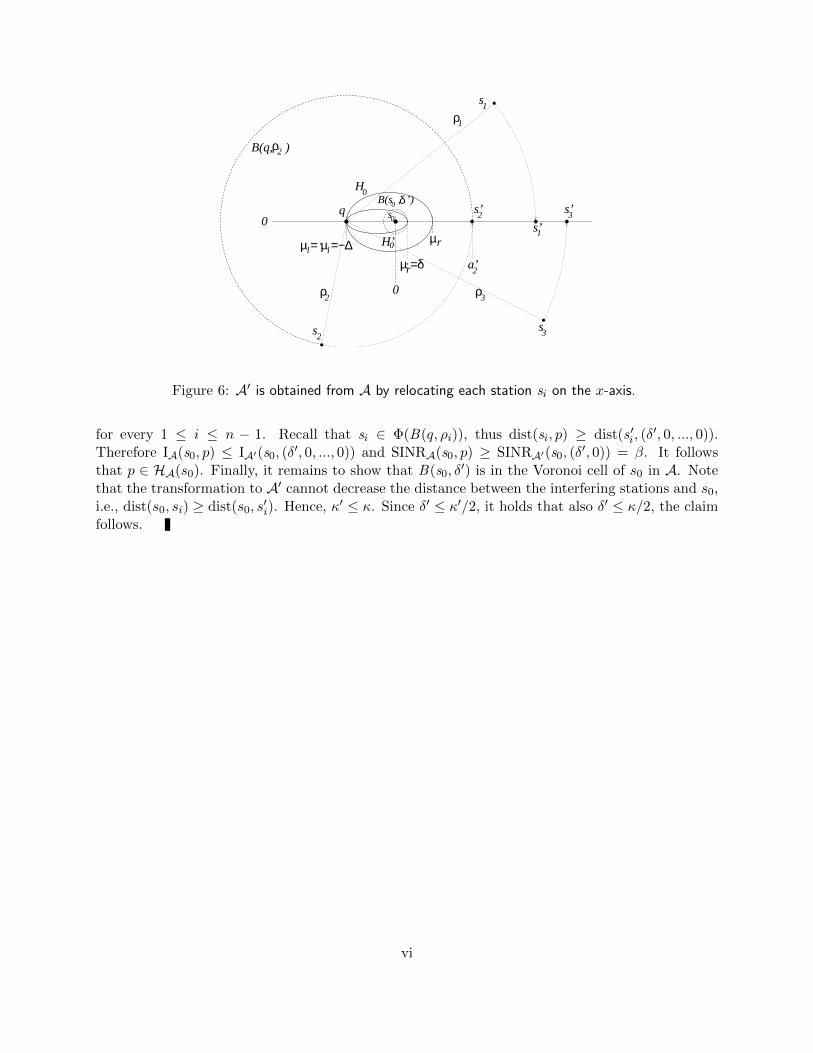
Figure 6: A′ is obtained from A by relocating each station si on the x-axis.

for every 1 ≤ i ≤ n − 1. Recall that si ∈ Φ(B(q, ρi)), thus dist(si, p) ≥ dist(s ′i, (δ′, 0, ..., 0)).

Therefore IA(s0, p) ≤ IA′(s0, (δ′, 0, ..., 0)) and SINRA(s0, p) ≥ SINRA′(s0, (δ

′, 0)) = β. It followsthat p ∈ HA(s0). Finally, it remains to show that B(s0, δ

′) is in the Voronoi cell of s0 in A. Notethat the transformation to A′ cannot decrease the distance between the interfering stations and s0,i.e., dist(s0, si) ≥ dist(s0, s

′i). Hence, κ′ ≤ κ. Since δ′ ≤ κ′/2, it holds that also δ′ ≤ κ/2, the claim

follows.

vi