Embed Size (px)
Citation preview
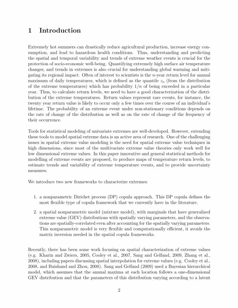
Nonparametric Spatial Models for Extremes:
Application to Extreme Temperature Data. ∗
Montserrat Fuentes, John Henry, and Brian Reich
SUMMARY
Estimating the probability of extreme temperature events is difficult because of limitedrecords across time and the need to extrapolate the distributions of these events, as opposedto just the mean, to locations where observations are not available. Another related issueis the need to characterize the uncertainty in the estimated probability of extreme events atdifferent locations. Although the tools for statistical modeling of univariate extremes are well-developed, extending these tools to model spatial extreme data is an active area of research.In this paper, in order to make inference about spatial extreme events, we introduce two newmodels. The first one is a Dirichlet-type mixture model, with marginals that have generalizedextreme value (GEV) distributions with spatially varying parameters, and the observationsare spatially-correlated even after accounting for the spatially varying parameters. Thismodel avoids the matrix inversion needed in the spatial copula frameworks, and it is verycomputationally efficient. The second is a Dirichlet prior copula model that is a flexiblealternative to parametric copula models such as the normal and t-copula. This presentsthe most flexible multivariate copula approach in the literature. The proposed modellingapproaches are fitted using a Bayesian framework that allow us to take into account differentsources of uncertainty in the data and models. To characterize the complex dependencestructure in the extreme events we introduce nonstationary (space-dependent) extremal-coefficient functions, and threshold-specific extremal functions. We apply our methods toannual maximum temperature values in the east-south-central United States.
∗M. Fuentes is a Professor of Statistics at North Carolina State University (NCSU). Tel.: (919) 515-1921,Fax: (919) 515-1169, E-mail: [email protected]. J. Henry is a postdoctoral fellow at the Department ofStatistics at NCSU. B. Reich is an Assistant Professor of Statistics at NCSU. The authors thank the Na-tional Science Foundation (Henry, DMS-0354189; Fuentes DMS-0706731, DMS-0353029), the EnvironmentalProtection Agency (Fuentes, R833863), and National Institutes of Health (Fuentes, 5R01ES014843-02) forpartial support of this work. Key words: dirichlet processes, extreme temperatures, nonstationarity, returnlevels, spatial models.
1
1 Introduction
Extremely hot summers can drastically reduce agricultural production, increase energy con-sumption, and lead to hazardous health conditions. Thus, understanding and predictingthe spatial and temporal variability and trends of extreme weather events is crucial for theprotection of socio-economic well-being. Quantifying extremely high surface air temperaturechanges, and trends in extremes is also crucial for understanding global warming and miti-gating its regional impact. Often of interest to scientists is the n-year return level for annualmaximum of daily temperatures, which is defined as the quantile zn (from the distributionof the extreme temperatures) which has probability 1/n of being exceeded in a particularyear. Thus, to calculate return levels, we need to have a good characterization of the distri-bution of the extreme temperatures. Return values represent rare events, for instance, thetwenty year return value is likely to occur only a few times over the course of an individual’slifetime. The probability of an extreme event under non-stationary conditions depends onthe rate of change of the distribution as well as on the rate of change of the frequency oftheir occurrence.
Tools for statistical modeling of univariate extremes are well-developed. However, extendingthese tools to model spatial extreme data is an active area of research. One of the challengingissues in spatial extreme value modeling is the need for spatial extreme value techniques inhigh dimensions, since most of the multivariate extreme value theories only work well forlow dimensional extreme values. In this paper innovative and general statistical methods formodelling of extreme events are proposed, to produce maps of temperature return levels, toestimate trends and variability of extreme temperature events, and to provide uncertaintymeasures.
We introduce two new frameworks to characterize extremes:
1. a nonparametric Dirichet process (DP) copula approach. This DP copula defines themost flexible type of copula framework that we currently have in the literature.
2. a spatial nonparametric model (mixture model), with marginals that have generalizedextreme value (GEV) distributions with spatially varying parameters, and the observa-tions are spatially-correlated even after accounting for the spatially varying parameters.This nonparametric model is very flexible and computationally efficient, it avoids thematrix inversion needed in the spatial copula frameworks.
Recently, there has been some work focusing on spatial characterization of extreme values(e.g. Kharin and Zwiers, 2005, Cooley et al., 2007, Sang and Gelfand, 2009, Zhang et al.,2008), including papers discussing spatial interpolation for extreme values (e.g. Cooley et al.,2008, and Buishand and Zhou, 2008). Sang and Gelfand (2009) used a Bayesian hierarchicalmodel, which assumes that the annual maxima at each location follows a one-dimensionalGEV distribution and that the parameters of this distribution varying according to a latent
2
spatial model capturing the spatial dependence. Nonstationarity refers to spatial dependencethat is a function of location, rather than just relative position of observations. To accountfor nonstationarity in univariate extreme events in an approach popularised by Davison andSmith (1999), the model parameters are modelled as functions of covariates. Eastoe andTawn (2009) and Eastoe (2009) suggest an alternative approach for spatial nonstationaryextremes: the nonstationarity in the whole dataset is first modelled and removed, usinga preprocessing technique. Then, the extremes of the pre-processed (transformed) dataare then modelled using the approach of Davison and Smith (1990), giving a model withboth pre-processing and tail parameters. We introduce here new continuous spatial modelsfor extreme values to account for spatial dependence which is unexplained by the latentspatial specifications for the distribution parameters, characterizing also the potential lackof stationarity across space and time. This is the first time that the pre-processing andtail-parameters are analyzed simultaneously using a fully Bayesian approach to account forall sources of uncertainty.
Although these methods in the literature for extremes would account for spatial correlationbetween nearby stations, the high-dimensional joint distributions induced by these modelsare restrictive. For example, we show that the Gaussian copula is asymptotically (as thethreshold increases) equivalent to the independence copula. In this work, we introduce non-parametric spatial frameworks to model extremes for annual maximum temperature, thatare flexible enough to characterize extreme events with complex spatio-temporal structures.Our nonparametric models have marginals that are GEVs, and are obtained using spatialstick-breaking (SB) approaches, that we describe next. The spatial nonparametric modelextends the stick-breaking (SB) prior of Sethuraman (1994), which is frequently used inBayesian modelling to capture uncertainty in the parametric form of an outcome’s distribu-tion. The SB prior is a special case of the priors neutral to the right (Doksum, 1974). Forgeneral (non-spatial) Bayesian modelling, the stick-breaking prior offers a way to model adistribution of a parameter as an unknown quantity to be estimated from the data. The
stick-breaking prior for the unknown distribution F, is Fd=∑m
i=1 piδ(Xi), where the number
of mixture components m may be infinite, pi = Vi
∏i−1j=1(1−Vj), Vi ∼ Beta(ai, bi) independent
across i, δ(Xi) is the Dirac distribution with point mass at Xi, Xiiid∼ Fo, and Fo is a known
distribution. A special case of this prior is the Dirichlet process prior with infinite m and
Viiid∼ Beta(1, ν) (Ferguson, 1973). The stick-breaking prior has been extended to the spatial
setting by incorporating spatial information into the either the model for the locations Xi
or the model for the masses pi, by Gelfand et al. (2005), Griffin and Steel (2006), Reich andFuentes (2007), Dunson and Park (2008), and An et al. (2009).
In this work we present measures to characterize complex spatial dependence in extreme tem-peratures, by allowing the extremal coefficient function, commonly used to study dependencestructure for max-stable models, to be space dependent.
This paper is organized as follows. In Section 2, we introduce a measure to characterizedependence in spatial extremes. In Section 3, we introduce an interesting result for theextremal coefficient of max-stable processes. In Section 4, we present copula-based spatial
3
extreme models, introducing a new copula framework, a DP copula. In Section 5, we presenta new nonparametric model for extremes with marginal distributions that are GEVs. InSection 6, we present some simulation studies to evaluate the performance of the new non-parametric models proposed here. In Section 7, we apply our methods to maximum annualtemperature data. We finish in Section 8 with some conclusions and final remarks.
2 Measures of spatial dependency for extremes
2.1 Max-stable processes
A stochastic process {Y (s), s ∈ D} is called max-stable if there exist constants ANs> 0, BNs
for N ≥ 1, s ∈ D ∈ R2, such that, if Y (1)(s), . . . Y (N)(s) are N independent copies of theprocess and
Y ∗(s) =
(
max1≤n≤NY(n)(s) −BNs
)
ANs
for s ∈ D. then, {Y ∗(s), s ∈ D} is identical in law to {Y (s), s ∈ D} .
If D is a finite set, this is the definition of a multivariate extreme value distribution (formaxima), and if |D| = 1, this reduces to the classical three types of Fisher and Tippett(see eg. Galambos, 1987). There is no loss of generality in transforming the margins to oneparticular extreme value distribution, and it is convenient to assume the standard Frechetdistribution,
P (Y (s) ≤ y) = e−1/y, (1)
for all s, in which case ANs= N , and BNs
= 0.
The generalised Extreme Value GEV distribution at each site s ∈ D, is given by
Fs(x;µ, σ, ψ) = exp
[
−{
1 − ξ(s)(x− µ(s))
σ(s)
}−1/ξ(s)
+
]
, (2)
where µ is the location parameter, σ is the scale, and ξ is the shape. The GEV distributionincludes three distributions as special cases (Fisher and Tippett, 1928):the Gumbel distri-bution if ξ → 0, the Frechet distribution with ξ > 0, and the Weibull with ξ < 0. Thedistribution’s domain also depends on ξ; the domain is (−∞,∞) if ξ = 0, (µ − σ/ξ,∞) ifξ > 0, and (−∞, µ− σ/ξ) if ξ < 0.
The probability integral transformation
y =
{
1 − ξ(s)(x− µ(s))
σ(s)
}1/ξ(s)
, (3)
4
has a standard Frechet distribution function (Fs(y) = e−1/y), so the transformation z = 1y
have an exponential with mean 1 distribution function, Fs(z) = 1−e−z. To simplify notation,throughout this paper we work with Frechet distributions, but in the application section, aspart of our hierarchical Bayesian framework we use the relationship between y and x given in3 at any given location s, to obtain the GEV distributions with space-dependent parameters.
To define a max-stable process, {Y (s)}, we consider that the marginal distribution has beentransformed to unit Frechet. Then, we impose that all the finite-dimensional distributionsare max-stable, i.e.
P (Y (s1) ≤ u1, . . . , Y (sm) ≤ um) = P t(Y (s1) ≤ tu1, . . . , Y (sm) ≤ tum)
for any t ≥ 0, m ≥ 1, s1, . . . , sm ∈ R2, ui > 0, with i = 1, . . . ,m.
2.2 Extremal coefficient
If the vector (Y (s1), . . . , Y (sm)) follows an m−variate extreme value distribution wherethe univariate margins are identically distributed, the extremal coefficient, θ, between sitess1, . . . , sm is given by
P (max(Y (s1), . . . , Y (sm)) < u) = (P (Y (s1) < u))θ
for all u ∈ R, where θ is independent of the value of u. The extremal coefficient wasintroduced by Smith (1990), see also Coles (1993), and Coles and Tawn (1996). Since, form i.i.d. random variables Y (s1), . . . , Y (sm)
P (max(Y (s1), . . . , Y (sm)) < u) = (P (Y (s1) < u))m
the extremal coefficient θ can be interpreted as the number of independent variables involvedin an m−variate distribution, and θ takes values in [1,m] where θ = 1 refers to completedependence.
2.3 Nonstationary extremal coefficient
The spatial dependency structure of extremes may change with location. In this section, weintroduce a nonstationary extremal coefficient function to characterize nonstationary spatialdependency structures in extremes.
We define a stationary extremal function, θ(s1, s2), as the extremal coefficient between lo-cations s1 and s2, that depends on s1 and s2 only through their vector distance s1 − s2, forany s1, s2 ∈ D. Thus,
P (max(Y (s1), Y (s2)) < 1) = (P (Y (s1) < 1))θ(s1,s2),
5
and there is a function θ0, such that,
θ(s1, s2) = θ0(s1 − s2).
This stationary extremal function was introduced by Schlather and Tawn, 2003. Here, weextend this function to a nonstationary setting.
A extremal function θ(s1, s2) that is a function of locations s1 and s2, is called in this papera nonstationary extremal function.
2.4 Threshold-specific extremal coefficient
Consider a extremal coefficient that satisfies
P (max(Y (s1), Y (s2)) < u) = (P (Y (s1) < u))θ(u),
and there is a function θ0, such that,
θ(u) = θ0(1),
for all u. Then, we name it a threshold-independent extremal coefficient.
A extremal coefficient θ(u) that depends on u is called in this paper a threshold-specific
extremal coefficient.
In general, we could have a nonstationary threshold-specific extremal function, θ, such that,
P (max(Y (s1), Y (s2)) < u) = (P (Y (s1) < u))θ(s1,s2;u).
We introduce in this paper models that would allow for nonstationary and threshold-specificdependency structure in the extremes.
3 Multivariate extreme distributions that are max-stable
A general method to construct a max-stable process is described by Smith (1990). Let{(ψi, xi, i ≥ 1)} denote the points of a Poison process on (0,∞) × S with intensity measureµ(dx×ds) = ψ−2dψ×ν(dx), where S is an arbitrary measurable set and ν a positive measureon S. Let {f(x, s), x ∈ S, s ∈ D} denote a non-negative function for which
∫
S
f(x, s)ν(dx) = 1,
6
for all s ∈ D. This construction is a result of the Pickands’ representation theorem (Pickands,1981) for multivariate extreme value distributions with unit Frechet margins, in which theintensity measure was written in terms of a positive finite measure H on the unit simplex,such that µ(dx× ds) = ψ−2dψ × dH(x).
Theoretically, the dependence structure of an m−variate extreme value distribution, can becharacterized by a certain positive measure H on a m−dimensional simplex. However, thismeasure H may have a complex structure and therefore cannot be easily inferred from data.
The extremal coefficient θ of Y (s1) and Y (s2) equals 2A(1/2), where A will depend on H(or alternatively on ν and f). For ν, the Lebesgue measure, and f(x, s) (as a function of sfor a fixed x) a multivariate normal density with mean x and covariance matrix Σ. Then, Ais defined as
A(w) = (1 − w)Φ (a/2 + 1/a log((1 − w)/w)) + wΦ (a/2 + 1/a log(w/(1 − w)))
where a = (s1 − s2)T Σ−1(s1 − s2) represents a generalised distance between the locations s1
and s2.
A new class of bivariate marginal distributions that are max-stable are defined by the ex-tremal Gaussian process, which is given by Schlather (2002),
− logP (Y (0) ≤ u, Y (s) ≤ v) =1
2
(
1
v+
1
u
)(
1 +
√
1 − 2(ρ(s) + 1)uv
(u+ v)2
)
where ρ is a stationary correlation function. This is an extension of Smith (1990)’s approach,by replacing the deterministic kernel function in Smith’s representation by a class of stochas-tic kernels that give a much richer class of processes that still have the max-stable property.The corresponding extremal coefficient between locations 0 and s would be
1 +
√
1 − 1
2(ρ(s) + 1),
which is a function of the vector distance between the two sites of interest. This could bemade nonstationary by introducing a correlation function that is space-dependent.
We introduce next an interesting result; max-stable processes are constrained to have thresh-old invariant dependence structure. This might not be a desirable property for spatial ex-tremes. For instance, with extreme temperatures, the dependence structure seems to bedifferent for cold years versus warmer years, this could suggest a threshold-specific depen-dence structure.
3.1 Theorem
Max-stable processes cannot have threshold-specific dependence structure.
7
Proof: We assume that {Y (s)} is a max-stable process. To define such a process, we considerthat the marginal distribution has been transformed to unit Frechet. Then, we impose thatall the finite-dimensional distributions are max-stable, i.e.
P (Y (s1) ≤ u1, . . . , Y (sm) ≤ um) = P t(Y (s1) ≤ tu1, . . . , Y (sm) ≤ tum)
for any t ≥ 0, m ≥ 1, s1, . . . , sm ∈ R2, ui > 0, with i = 1, . . . ,m. Then, the extremalcoefficient is given by
θ = −u log{P (Y (s1) ≤ u, . . . , Y (sm) ≤ u)}
but, P (Y (s1) ≤ u, . . . , Y (sm) ≤ u) = P t(Y (s1) ≤ tu, . . . , Y (sm) ≤ tu) for any t ≥ 0.Therefore,
θ(u) = −u log{P (Y (s1) ≤ u, . . . , Y (sm) ≤ u)} (4)
= −ut log{P (Y (s1) ≤ ut, . . . , Y (sm) ≤ ut)} = θ(ut),
for any t ≥ 0. θ(u) = θ(1) for all u. Thus, the extremal coefficient is threshold invariant. 2
In the next section we introduce a nonparametric extension of the copula approach that canbe used to generate non-stationary dependence structure in extremes and threshold-specificextremal functions.
4 Copula-based multivariate extreme models
4.1 Gaussian copula
The Gaussian copula function (e.g. Nelsen, 1999) is defined as Cρ(u, v) = Φρ(Φ−1(u),Φ−1(v)),
where u, v ∈ [0, 1], Φ denotes the standard normal cumulative distribution function (CDF),and Φρ denotes the CDF of the standard bivariate Gaussian distribution with correlationρ. If we use a Gaussian copula to characterize the bivariate dependence structure between ex-
tremes at two locations s1 and s2, then, we have (Y (s1), Y (s2))d=(
G−1s1
Φ(Z(s1)), G−1s2
Φ(Z(s2)))
where Z(s1) and Z(s2) are standard normal r.v.s with correlation ρ, and G−1s1
and G−1s2
arethe inverse marginal distribution functions for Y (s1) and Y (s2). The distribution functionof (Y (s1), Y (s2)) is given by H(Y (s1), Y (s2), ρ) = Φρ(Gs1
(Y (s1), Gs2(Y (s2)). The marginal
distributions of Y (s1) and Y (s2) remain Gs1and Gs2
.
Throughout this copula section, to simplify notation we assume the marginal distributionsfor Y (s), with s ∈ D are Frechet. However, without lack of generality using the relationshipin (3), we allow the marginal distributions to be a GEV with space-dependent parameters.Then, the extremal coefficient would be given by
P (max(Y (s1), Y (s2)) < 1) = (P (Y (s1) < 1))θ,
8
and we obtainθ = −log
(
Φρ(Φ−1Gs1
(1),Φ−1Gs2(1); ρ
)
where Φ−1 is the inverse distribution function of N(0, 1).
4.2 Spatial Gaussian copula
We generalize the bivariate case (with two sites, s1 and s2), to a set of sites {s1, . . . , sm},using a spatial copula; good references for multivariate copulas are Joe (1997), and Nelsen(1999). The spatial copula introduces a latent Gaussian process R(s) with mean zero, unitvariance, and spatial covariance cov(R(s1), R(s2)) = ρR(s1, s2). FR denotes the multivariatedistribution function MVN(0,Σ), where Σ = [ρ(si, sj)]
mi,j=1, of the spatial process R. Then
T (s)(def)= Φ(R(s)) ∼ Unif(0,1). To relate the latent and data processes, let G be the CDF of
the standard Frechet distribution. Then,
Y (s) = G−1(T (s)) ∼ G. (5)
T (s) determines the Y (s)’s percentile, and since the T (s) have spatial correlation (via R(s)),the outcomes also have spatial correlation. Given the correlation function ρR of the latentprocess R we can derive the Gaussian copula CR for the distribution function of R
CR(u1, . . . , um) = FR(Φ−1(u1), . . . ,Φ−1(um)),
where (u1, . . . , um) ∈ [0, 1]m. Let FY denote the multivariate distribution of Y , then
FY (y1, . . . , ym) = CR(G(y1), . . . , G(ym)) = FR(Φ−1G(y1), . . . ,Φ−1G(ym)), (6)
where (y1, . . . , ym) ∈ Rm.
If the spatial covariance ρR is stationary, i.e. cov(R(s1), R(s2)) = ρR(s1 − s2) then theresulting extremal function between s1 and s2 will be also stationary. Since,
θ(s1, s2) = θ0(s1 − s2) = −log(
FR(Φ−1Gs1(1),Φ−1Gs2
(1))
,
only depends on s1 and s2 through its vector distance, because FR has a stationary covariance.
If the spatial covariance ρR is nonstationary, this can be achieved by, for instance, usingthe nonstationary model for the covariance of R that is presented in Section 7.2, then theresulting extremal function is nonstationary
θ(s1, s2) = −log(
FR(Φ−1Gs1(1),Φ−1Gs2
(1))
),
since the covariance of R is nonstationary.
The extremal function could be also made threshold-specific,
θ(s1, s2;u) = −ulog(
FR(Φ−1Gs1(u),Φ−1Gs2
(u))
),
9
4.3 Multivariate copulas that are max-stable
A spatial copula C satisfying the relationship
C(ur1, . . . , u
rm) = Cr(u1, . . . , um) (7)
for all r > 0 will be called a spatial extreme value copula. If H is a m-variate spatialdistribution with copula C, such as it satisfies (7), and the marginals of H have a GEVdistribution, then H is a multivariate Extreme Value distribution. In the literature, (7) isknown as max-stability property for copulas. The spatial Gaussian copula does not satisfy(7). The Gumbel-Hougaard m-copula, defined as
Cτ (u1, . . . , um) = exp−[(− log u1)τ + · · · + (− log um)τ ]1/τ ,
for τ ≥ 1, and the independent copula,
C(u1, . . . , um) = Πmi=1ui, (8)
would be extreme values copulas, and they are threshold-invariant. Dependency in theGumbel-Hougaard m-copula could be introduced via the parameter τ.
For the Gumbel-Hougaard m-copula, the threshold-invariant extremal coefficient is
θ = m1/τ .
Thus, τ is a measure of the dependency of the extremes, the limiting case τ → 1, correspondsto independence between the variables, whereas the limit case τ → ∞ correspond to completedependence. By making τ space-dependent, we can obtain a nonstationary dependency forthe extremes. First, we define a Gumbel-Hougaard 2-copula
Cτ(s1,s2)(u1, u2) = exp−[(− log u1)τ(s1,s2) + (− log u2)
τ(s1,s2)]1/τ(s1,s2),
where τ(s1, s2) is a measure of the strength of the dependency between sites s1 and s2.
Then, the extremal bivariate nonstationary function (threshold-invariant) θ is given by
θ(s1, s2;u) = 21/τ(s1,s2).
Generalizing this result from from the bivariate setting to a multivariate setting for spatialdata is more challenging, and very computationally demanding. However, we present nexta nonparametric approach that introduces more flexibility and allows for threshold-specificand nonstationarity in the extremal function, we refer to it as a Dirichlet process copulamodel.
10
4.4 Limiting copula for the Gaussian copula
Consider iid random vectors Y(1), . . . ,Y(N), where Y(i) = (Y (i)(s1), . . . , Y(i)(sm)), with dis-
tribution function F , and define MN the vector of the componentwise maxima (the jth
component of MN is the maximum of the jth component over all N observations). We saythat F is in the maximum domain of attraction (eg. Nasri-Roudsari, 1996) of the distributionfunction H, if there exist sequences of vectors AN > 0 and BN ∈ Rd, such that
limN→∞
P
(
MN,1 −BN1
AN,1
≤ y1, . . . ,MN,d −BNm
AN,d
≤ ym
)
= limn→∞
FN(ANy + BN) = H(y).
A non-degenerate limiting distribution H is known as a multivariate extreme value distribu-tion. The unique copula C0 of the limit H is an EV copula.
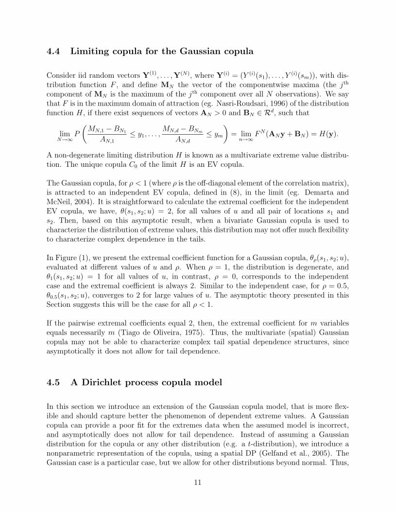
The Gaussian copula, for ρ < 1 (where ρ is the off-diagonal element of the correlation matrix),is attracted to an independent EV copula, defined in (8), in the limit (eg. Demarta andMcNeil, 2004). It is straightforward to calculate the extremal coefficient for the independentEV copula, we have, θ(s1, s2;u) = 2, for all values of u and all pair of locations s1 ands2. Then, based on this asymptotic result, when a bivariate Gaussian copula is used tocharacterize the distribution of extreme values, this distribution may not offer much flexibilityto characterize complex dependence in the tails.
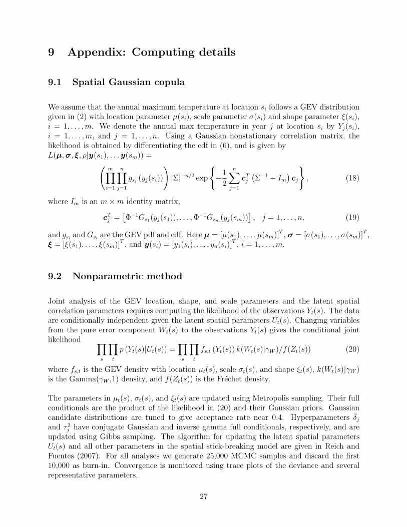
In Figure (1), we present the extremal coefficient function for a Gaussian copula, θρ(s1, s2;u),evaluated at different values of u and ρ. When ρ = 1, the distribution is degenerate, andθ1(s1, s2;u) = 1 for all values of u, in contrast, ρ = 0, corresponds to the independentcase and the extremal coefficient is always 2. Similar to the independent case, for ρ = 0.5,θ0.5(s1, s2;u), converges to 2 for large values of u. The asymptotic theory presented in thisSection suggests this will be the case for all ρ < 1.
If the pairwise extremal coefficients equal 2, then, the extremal coefficient for m variablesequals necessarily m (Tiago de Oliveira, 1975). Thus, the multivariate (spatial) Gaussiancopula may not be able to characterize complex tail spatial dependence structures, sinceasymptotically it does not allow for tail dependence.
4.5 A Dirichlet process copula model
In this section we introduce an extension of the Gaussian copula model, that is more flex-ible and should capture better the phenomenon of dependent extreme values. A Gaussiancopula can provide a poor fit for the extremes data when the assumed model is incorrect,and asymptotically does not allow for tail dependence. Instead of assuming a Gaussiandistribution for the copula or any other distribution (e.g. a t-distribution), we introduce anonparametric representation of the copula, using a spatial DP (Gelfand et al., 2005). TheGaussian case is a particular case, but we allow for other distributions beyond normal. Thus,
11
this approach is flexible enough to characterize the potentially complex spatial structuresof the extreme values. This DP model provides a random joint distribution for a stochasticprocess of random variables. The fitting of this type of DP model is fairly straightforwardusing Markov chain Monte Carlo (MCMC) methods. This DP copula defines a more flexiblecopula than currently available in the literature.
The spatial Dirichlet process copula introduces a latent process Zt, such that in year t, fort = 1, . . . , T, the joint density of Zt = (Zt(s1), . . . , Zt(sm)) at m locations (s1, . . . , sm), given,Hm, the m-random probability measure of the spatial part (m-variate normal) and τ 2, thenugget component, f(Z|Hm, τ 2), is almost surely of the form (this is a conditional density)
fZt=
∞∑
i=1
piNm(Z|θi, τ2Im), (9)
where the vector θi = (θi(s1), . . . , θi(sm)), pi = Vi
∏
j<i(1 − Vj), Vi ∼ Beta(1, ν),
θt,i|Hm ∼ind Hm, t = 1, ...T,
and Hm = DP (νHm0 ), Hm
0 = Nm(.|0m,Σ). We denote FZ the distribution of Z associatedto the density in (9) (a countable mixture of normals).
Then, Tt(s) = H(Zt(s)) ∼ Unif(0, 1), where Hs is the CDF for Zt(s),
Hs =∞∑
i=1
piΦ(θi(s)).
The copula CZ for the distribution function of Zt(s1), . . . , Zt(sm) is (conditioning on the θi
components),CZt
(u1, . . . , um) = FZt(H−1
s1(u1), . . . , H
−1sm
(um)),
where u1, . . . um ∈ [0, 1]m. Then, Yt(s) ∼ G−1(Tt(s)) ∼ G. G is the CDF of the standardFrechet distribution. Using the relationship in (3), we allow the marginal distributions tobe GEVs with space-dependent parameters, by incorporating a change of variable (y to x in(3)) in the likelihood function (see appendix). The multivariate distribution of Yt is
FYt(y1, . . . , ym) = CZt
(G(y1), . . . , G(ym)).
Spatial dependence for spatial extremes using the DP copula.
If the spatial covariance Σ in fZ is nonstationary, then the resulting extremal function isnonstationary
θ(s1, s2) = −log(
FZt(H−1
s1G(1), H−1
s2G(1)
)
),
since the covariance Σ in FZtis nonstationary. The extremal function could be also made
threshold-specific,
θ(s1, s2;u) = −ulog(
FZt(H−1
s1G(u), H−1
s2G(u)
)
).
12
Since FZ is a multivariate distribution, the results above can be extended and calculatedsimultaneously for any number of sites {s1, . . . , sm}.
In Figure 1 we present the extremal coefficient for a copula that is a mixture of normaldistributions. This is a simplified version of the mixture copula proposed in this section,we present it here as an illustration of the flexibility that this mixture copula frameworkoffers to explain tail dependence structures. The mixture copula density in Figure 1 is∑M
j=1 pjN2(x|µj12,Σj) where M = 10, x is a 2-vector, µ is a 10-dimensional vector with
equally spaced values between −3 and 3, the jth component of µ is µj, the weights are pj =1/M, and Σj is the correlation matrix with off-diagonal element ρj. The two mixture copulasin Figure (1) have either ρ = (0, . . . , 1), where ρ is a 10-dimensional vector with equallyspaced values between 0 and 1, such as the jth component of ρ is ρj, and ρ = (1, . . . , 0). Inone case the extremal coefficient increases for large values of u, while in the other we havethe reverse situation, that a Gaussian copula could not characterize. As we increase M weallow for more flexibility in the tail dependence, ultimately, in the mixture presented in thisSection with M = ∞, we can obtain all different type of shapes for the extremal coefficientas a function of u. Though in practice, it might be useful to consider finite approximations tothe infinite stick-breaking process. Dunson and Park (2008) study the asymptotic propertiesof truncation approximations to the infinite mixture, while Papaspiliopoulos and Roberts(2008) introduce an elegant computational approach to work with an infinite mixture forDirichlet processes mixing.
5 Nonparametric approach
In this section we extend common statistical models for extreme data to the spatial settingusing a nonparametric approach. We make two important modifications to analyze extremetemperature events. In Cooley et al. (2007), the scale and shape parameters of the general-ized pareto (GP) distribution are allowed to vary with space and time. The same idea is usedhere, where we allow the locations, scale, and shape parameters of the generalized extremevalue distribution to vary with space and time (see (3)). This allows us to identify locationsthat are more likely to experience extreme events and to monitor changes in the frequency ofextreme events. Second, we model the spatial residual associations at nearby observations.Extremes for high temperature often display strong spatial patterns. Accounting for residualcorrelation is crucial to obtaining reasonable measures of uncertainty for estimates of returnlevels. To our knowledge, this is the first spatio-temporal model for extremes that allowsfor residual correlation, and the first time that the pre-processing and tail-parameters areanalyzed simultaneously using a fully Bayes approach to account for all different sources ofuncertainty.
We introduce a new method to account for spatial correlation, while the data’s marginaldistribution is assumed to be a common extreme model, such as the GEV. Given the ab-sence of work that has been done in this area, it is important to develop new methods and
13
investigate their properties. The mixture approach is computationally convenient becauseit avoids matrix inversion (needed in the spatial copula approaches), which is crucial foranalyzing large data sets. Also, it is straight-forward to allow for nonstationarity in thespatial correlation by allowing the bandwidths to vary spatially.
We assume Yt(s) has a standard Frechet distribution (we use relationship in (3) to obtaina GEV with space-dependent parameters), for all s ∈ D. We introduce the transformationz = 1/y, then Zt(s) has an Expo(1) distribution. We model Zt(s) = Ut(s) + Wt(s), whereWt is a pure error term with a Gamma(γW , 1) distribution. We assign a nonparametric priorfor the distribution of Ut, e.g. a stick breaking prior (Reich and Fuentes, 2007), FUt(s) =∑M
i=1 pi(s)δ(τi), where τi has a Gamma(γU , 1) distribution, with γU + γW = 1, and pi(s) isthe probability mass at location s that is modelled using kernel functions. Reich and Fuentes(2007) assume the τi are draws from independent normal distributions, here we assume aGamma distribution to obtain the GEV marginals. We have pi(s) = Vi(s)
∏i−1j=1(1 − Vj(s)),
and Vi(s) = wi(s)Vi. The distributions FUt(s) are related through their dependence onthe Vi and τi, which are given the priors Vi ∼ Beta(1, ν) and τi ∼ Gamma(γU , 1), eachindependent across i. However, the distributions vary spatially according to the kernelfunctions wi(s), which are restricted to the interval [0, 1]. The function wi(s) is centeredat knot ψi = (ψ1i, ψ2i) and the spread is controlled by the bandwidth parameter λi. Boththe knots and the bandwidths are modelled as unknown parameters. The knots ψi are givenindependent uniform priors over the spatial domain (this could generalized). The bandwidthscan be modelled as equal for each kernel function or varying across kernel functions. Aconvenient feature of this mixture model is that we allow the amount of spatial correlationto vary spatially by adding a spatial prior for the bandwidths of the kernel stick-breakingprobabilities pi(s). This results in an extremely flexible class of models, since by using kernelfunctions with bandwidth parameters that are space-dependent, we allow for nonstationarityin the extremal function.
The joint distribution for Zt = (Zt(s1), . . . , Zt(sm)) is
F (Zt|FUt, γW ) =
∫
Gamma(Zt − Ut|γW )FU(dUt)
where Gamma(·|γW ), denotes a Gamma(γW , 1) distribution, Ut = Ut(s1), . . . , Ut(sm). Then,the joint density of Zt(s1) and Zt(s2) is given by
f(Zt(s1), Zt(s2)|FUt(s1),Ut(s2), γW ) =
∫
k(Zt(s1) − Ut(s1)|γW )k(Zt(s2) − Ut(s2)|γW )FUt(s1),Ut(s2)(d(Ut(s1), Ut(s2)))
where, given the τi’s and γW is almost surely of the form,
∑
i
pi(s1)pi(s2)k(Zt(s1) − τi|γW )k(Zt(s2) − τi|γW )
where k(.|γW ) is the density of a Gamma(γW , 1) distribution.
14
To investigate the induced relationship between pairs of locations, we calculate the extremalcoefficient. We have
P (Yt(s1) < 1, Yt(s2) < 1) = P (Zt(s1) > 1, Zt(s2) > 1),
where,
P (Zt(s1) > 1, Zt(s2) > 1|Vi, ψi, λi, τi, γW ) =
∫ ∞
1
∫ ∞
1
∑
i
pi(s1)pi(s2)k(z1−τi|γW )k(z2−τi|γW )dz1dz2.
Thus, we have
P (Zt(s1) > 1, Zt(s2) > 1|Vi, ψi, λi, τi, γW ) =∑
i
pi(s1)pi(s2)(
∫ ∞
1
k(z − τi|γW )dz)2
=
(
∑
i
pi(s1)pi(s2)γ2I (γW , 1 − τi)
)
/Γ2(γW ), (10)
where γI() is the (upper) incomplete gamma function. Taking expectations in (10) withrespect to the τ ′i components, we obtain
∑
i
pi(s1)pi(s2)
∫ ∞
0
γ2I (γW , 1 − x)k(x|γU)dx/Γ2(γW ). (11)
Expression (11) depends on locations s1 and s2 only through the expression∑
i pi(s1)pi(s2),that could be written as
∑
i
pi(s1)pi(s2)
=∞∑
i=1
[
wi(s1)wi(s2)V2i
∏
j<i
(
1 − (wj(s1) + wj(s2))Vj + wj(s1)wj(s2)V2j
)
]
. (12)
Integrating over the (Vi, ψi, λi), equation (12) becomes
c2v2
∑
i
[1 − 2c1v1 + c2v2]i−1
where Vi ∼ Beta(a, b), v1 = E(V1), v2 = E(V 21 ), c1 =
∫ ∫
wi(s1)p(ψi, λi)dψdλi, and c2 =∫ ∫
wi(s1)wi(s2)p(ψi, λi)dψdλi. we apply the formula for the sum of a geometric series andsimplify, leaving
c2v2
2c1v1 − c2v2
=γ(s1, s2)
2(
1 + ba+1
)
− γ(s1, s2), (13)
where γ(s1, s2) = c2/c1. This is a spatial stationary function for certain choices of kernelfunctions.
Then, the conditional extremal coefficient is
θ(s1, s2) = −2 log(Γ(γW ))/ log(1 − e−1)
+ log
(
γ(s1, s2)
2(
1 + ba+1
)
− γ(s1, s2)
∫ ∞
0
γ2I (γW , 1 − x)k(x|γU)dx
)
/ log(1 − e−1),
15
γ(s1, s2) is a spatial stationary function for certain kernel functions, and the extremal func-tion would be then stationary. By allowing the kernel function to be space-dependence weintroduce nonstationarity.
In our model we also allow the extremal function to be threshold specific,
θ(s1, s2; l) = −2 log(Γ(γW ))/ log(1 − e−1/l)
+ log
(
γ(s1, s2)
2(
1 + ba+1
)
− γ(s1, s2)
∫ ∞
0
γ2I (γW , l + x)k(x|γU)dx
)
/ log(1 − e−1/l).
6 Simulated examples
In this section we conduct a brief simulation study to demonstrate the ability of Section5’s nonparametric approach to accommodate nonstationarity and to test for sensitivity tohyperprior choice. We generate two simulated data sets, each with nt = 10 replicates at eachof ns = 100 spatial locations. The spatial locations si = (si1, si2) are generated uniformly on[0, 1]2. For both data sets the nt replicates are independent and identically distributed withGEV marginals with µt(s) = αµ(s) = 20∗ (s1 − .5)2, scale σ(s) = exp (βµ(s)) ≡ 1, and shapeξt(s) = ασ(s) ≡ −0.1. The observations for the first data set are independent across space.The second data set is generated from the nonstationary Gaussian copula with covariancematrix Σ, having (i, j)th element
Σij =√si2sj2 exp(−||si − sj||) +
√
(1 − si2)(1 − sj2)I(i = j).
The covariance has variance one across space and stronger spatial correlation in areas witha large second coordinate.
The spatial processes δj, j = 1, ..., 3, have independent spatial Gaussian priors with mean δj
and covariance τ 2j exp(−||si − sj||/ρj). We use priors δj
iid∼ N(0,102), τ−2j
iid∼ Gamma(0.1,0.1)
(parameterized to have mean one and variance ten), and ρjiid∼ Gamma(0.1,0.1). This prior
for ρj induces prior median 0.57 and prior 95% interval (0.00,0.95) for exp(−0.25/ρj), thecorrelation between two points with ||si − sj|| = 0.25. We use squared-exponential kernels,exp(−0.5(s−ψi)
′(s−ψi)/λ2i ), where the knots ψi have independent uniform priors over the
spatial domain, and the bandwidth parameters λi have independent exponential priors, λiiid∼
Expo(λ0), λ0 is the prior mean of the bandwidth parameters and it has a Gamma(0.1,0.1)prior. We truncate the mixture model at M = 50 terms, and assume ν has a Gamma(0.1,0.1)prior, where ν is the parameter for the Vi components, such that Vi ∼ Beta(1, ν).
The parameter γU controls the relative contribution of the spatial and nonspatial componentsof the latent stick-breaking process, with large γU indicating strong spatial correlation. Table1 shows that the γU ’s posterior median for the first data set generated without residual spatial
16
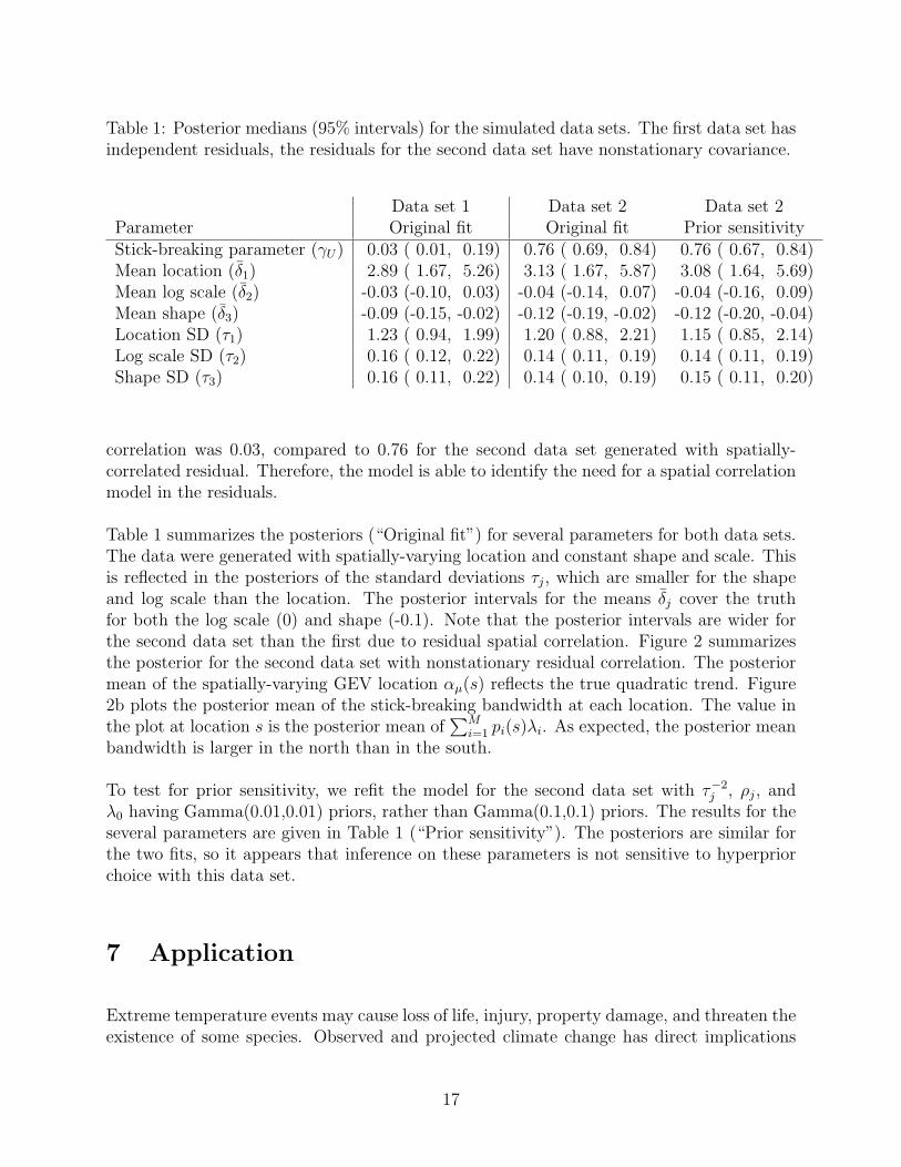
Table 1: Posterior medians (95% intervals) for the simulated data sets. The first data set hasindependent residuals, the residuals for the second data set have nonstationary covariance.
Data set 1 Data set 2 Data set 2Parameter Original fit Original fit Prior sensitivityStick-breaking parameter (γU) 0.03 ( 0.01, 0.19) 0.76 ( 0.69, 0.84) 0.76 ( 0.67, 0.84)Mean location (δ1) 2.89 ( 1.67, 5.26) 3.13 ( 1.67, 5.87) 3.08 ( 1.64, 5.69)Mean log scale (δ2) -0.03 (-0.10, 0.03) -0.04 (-0.14, 0.07) -0.04 (-0.16, 0.09)Mean shape (δ3) -0.09 (-0.15, -0.02) -0.12 (-0.19, -0.02) -0.12 (-0.20, -0.04)Location SD (τ1) 1.23 ( 0.94, 1.99) 1.20 ( 0.88, 2.21) 1.15 ( 0.85, 2.14)Log scale SD (τ2) 0.16 ( 0.12, 0.22) 0.14 ( 0.11, 0.19) 0.14 ( 0.11, 0.19)Shape SD (τ3) 0.16 ( 0.11, 0.22) 0.14 ( 0.10, 0.19) 0.15 ( 0.11, 0.20)
correlation was 0.03, compared to 0.76 for the second data set generated with spatially-correlated residual. Therefore, the model is able to identify the need for a spatial correlationmodel in the residuals.
Table 1 summarizes the posteriors (“Original fit”) for several parameters for both data sets.The data were generated with spatially-varying location and constant shape and scale. Thisis reflected in the posteriors of the standard deviations τj, which are smaller for the shapeand log scale than the location. The posterior intervals for the means δj cover the truthfor both the log scale (0) and shape (-0.1). Note that the posterior intervals are wider forthe second data set than the first due to residual spatial correlation. Figure 2 summarizesthe posterior for the second data set with nonstationary residual correlation. The posteriormean of the spatially-varying GEV location αµ(s) reflects the true quadratic trend. Figure2b plots the posterior mean of the stick-breaking bandwidth at each location. The value inthe plot at location s is the posterior mean of
∑Mi=1 pi(s)λi. As expected, the posterior mean
bandwidth is larger in the north than in the south.
To test for prior sensitivity, we refit the model for the second data set with τ−2j , ρj, and
λ0 having Gamma(0.01,0.01) priors, rather than Gamma(0.1,0.1) priors. The results for theseveral parameters are given in Table 1 (“Prior sensitivity”). The posteriors are similar forthe two fits, so it appears that inference on these parameters is not sensitive to hyperpriorchoice with this data set.
7 Application
Extreme temperature events may cause loss of life, injury, property damage, and threaten theexistence of some species. Observed and projected climate change has direct implications
17
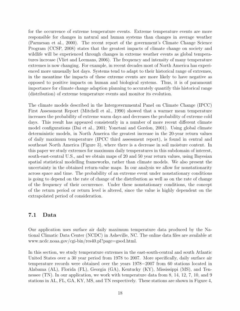
for the occurrence of extreme temperature events. Extreme temperature events are moreresponsible for changes in natural and human systems than changes in average weather(Parmesan et al., 2000). The recent report of the government’s Climate Change ScienceProgram (CCSP, 2008) states that the greatest impacts of climate change on society andwildlife will be experienced through changes in extreme weather events as global tempera-tures increase (Vliet and Leemans, 2006). The frequency and intensity of many temperatureextremes is now changing. For example, in recent decades most of North America has experi-enced more unusually hot days. Systems tend to adapt to their historical range of extremes,in the meantime the impacts of these extreme events are more likely to have negative asopposed to positive impacts on human and biological systems. Thus, it is of paramountimportance for climate change adaption planning to accurately quantify this historical range(distribution) of extreme temperature events and monitor its evolution.
The climate models described in the Intergovernmental Panel on Climate Change (IPCC)First Assessment Report (Mitchell et al., 1990) showed that a warmer mean temperatureincreases the probability of extreme warm days and decreases the probability of extreme colddays. This result has appeared consistently in a number of more recent different climatemodel configurations (Dai et al., 2001; Yonetani and Gordon, 2001). Using global climatedeterministic models, in North America the greatest increase in the 20-year return valuesof daily maximum temperature (IPCC third assessment report), is found in central andsoutheast North America (Figure 3), where there is a decrease in soil moisture content. Inthis paper we study extremes for maximum daily temperatures in this subdomain of interest,south-east-central U.S., and we obtain maps of 20 and 50 year return values, using Bayesianspatial statistical modelling frameworks, rather than climate models. We also present theuncertainty in the obtained return-value maps. In our analysis we allow for nonstationarityacross space and time. The probability of an extreme event under nonstationary conditionsis going to depend on the rate of change of the distribution as well as on the rate of changeof the frequency of their occurrence. Under these nonstationary conditions, the conceptof the return period or return level is altered, since the value is highly dependent on theextrapolated period of consideration.
7.1 Data
Our application uses surface air daily maximum temperature data produced by the Na-tional Climatic Data Center (NCDC) in Asheville, NC. The online data files are available atwww.ncdc.noaa.gov/cgi-bin/res40.pl?page=gsod.html.
In this section, we study temperature extremes in the east-south-central and south AtlanticUnited States over a 30 year period from 1978 to 2007. More specifically, daily surface airtemperature records were obtained over the years 1978−2007 from 60 stations located inAlabama (AL), Florida (FL), Georgia (GA), Kentucky (KY), Mississippi (MS), and Ten-nessee (TN). In our application, we work with temperature data from 8, 14, 12, 7, 10, and 9stations in AL, FL, GA, KY, MS, and TN respectively. These stations are shown in Figure 4,
18
and are located within the region with the greatest increase in 20-year return values of dailymaximum temperature (see Figure 3) according to the Intergovernmental Panel on ClimateChange (IPCC) Third Assessment Report “Climate change 2001”.
In the following two sections we present different statistical methods to characterize spatialnonstationary dependence in extreme temperature values. First, using a copula framework(as in Section 4), and then using a nonparametric approach (as in Section 5).
7.2 Copula approach
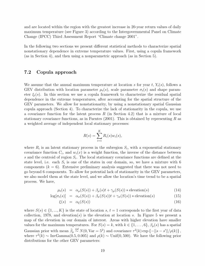
We assume that the annual maximum temperature at location s for year t, Yt(s), follows aGEV distribution with location parameter µt(s), scale parameter σt(s) and shape param-eter ξt(s). In this section we use a copula framework to characterize the residual spatialdependence in the extreme temperatures, after accounting for the spatial structure of theGEV parameters. We allow for nonstationarity, by using a nonstationary spatial Gaussiancopula approach (Section 4). To characterize the lack of stationarity in the copula, we usea covariance function for the latent process R (in Section 4.2) that is a mixture of localstationary covariance functions, as in Fuentes (2001). This is obtained by representing R asa weighted average of independent local stationary processes:
R(s) =K∑
i=1
Ri(s)wi(s),
where Ri is an latent stationary process in the subregion Si, with a exponential stationarycovariance function Ci, and wi(x) is a weight function, the inverse of the distance betweens and the centroid of region Si. The local stationary covariance functions are defined at thestate level, i.e. each Si is one of the states in our domain, so, we have a mixture with 6components (k = 6). Extensive preliminary analysis suggested that there was not need togo beyond 6 components. To allow for potential lack of stationarity in the GEV parameters,we also model them at the state level, and we allow the location’s time trend to be a spatialprocess. We have,
µt(s) = αµ(S(s)) + βµ(s)t+ γµ(S(s)) ∗ elevation(s) (14)
log[σt(s)] = ασ(S(s)) + βσ(S(s))t+ γσ(S(s)) ∗ elevation(s) (15)
ξ(s) = αξ(S(s)) (16)
where S(s) ∈ {1, ..., K} is the state of location s, t = 1 corresponds to the first year of datacollection, 1978, and elevation(s) is the elevation at location s. In Figure 5 we present amap of the elevation in our domain of interest. Areas with higher elevation have smallervalues for the maximum temperatures. For S(s) = k, with k ∈ {1, . . . , 6}, βµ(s) has a spatial
Gaussian prior with mean βµiid∼ N(0,Var = 52) and covariance τ 2(k) exp {−||s− s′||/ρ(k)} ,
where τ 2(k) ∼ InvGamma(0.5, 0.005) and ρ(k) ∼ Unif(0, 500). We have the following priordistributions for the other GEV parameters:
19
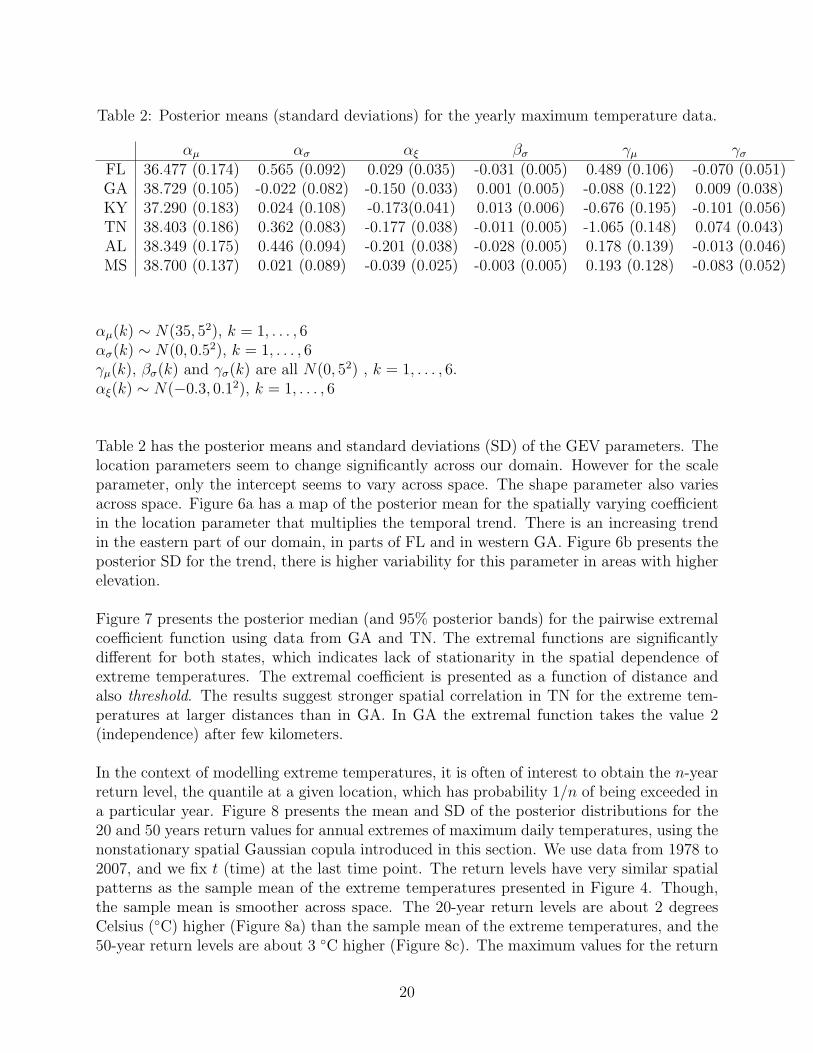
Table 2: Posterior means (standard deviations) for the yearly maximum temperature data.
αµ ασ αξ βσ γµ γσ
FL 36.477 (0.174) 0.565 (0.092) 0.029 (0.035) -0.031 (0.005) 0.489 (0.106) -0.070 (0.051)GA 38.729 (0.105) -0.022 (0.082) -0.150 (0.033) 0.001 (0.005) -0.088 (0.122) 0.009 (0.038)KY 37.290 (0.183) 0.024 (0.108) -0.173(0.041) 0.013 (0.006) -0.676 (0.195) -0.101 (0.056)TN 38.403 (0.186) 0.362 (0.083) -0.177 (0.038) -0.011 (0.005) -1.065 (0.148) 0.074 (0.043)AL 38.349 (0.175) 0.446 (0.094) -0.201 (0.038) -0.028 (0.005) 0.178 (0.139) -0.013 (0.046)MS 38.700 (0.137) 0.021 (0.089) -0.039 (0.025) -0.003 (0.005) 0.193 (0.128) -0.083 (0.052)
αµ(k) ∼ N(35, 52), k = 1, . . . , 6ασ(k) ∼ N(0, 0.52), k = 1, . . . , 6γµ(k), βσ(k) and γσ(k) are all N(0, 52) , k = 1, . . . , 6.αξ(k) ∼ N(−0.3, 0.12), k = 1, . . . , 6
Table 2 has the posterior means and standard deviations (SD) of the GEV parameters. Thelocation parameters seem to change significantly across our domain. However for the scaleparameter, only the intercept seems to vary across space. The shape parameter also variesacross space. Figure 6a has a map of the posterior mean for the spatially varying coefficientin the location parameter that multiplies the temporal trend. There is an increasing trendin the eastern part of our domain, in parts of FL and in western GA. Figure 6b presents theposterior SD for the trend, there is higher variability for this parameter in areas with higherelevation.
Figure 7 presents the posterior median (and 95% posterior bands) for the pairwise extremalcoefficient function using data from GA and TN. The extremal functions are significantlydifferent for both states, which indicates lack of stationarity in the spatial dependence ofextreme temperatures. The extremal coefficient is presented as a function of distance andalso threshold. The results suggest stronger spatial correlation in TN for the extreme tem-peratures at larger distances than in GA. In GA the extremal function takes the value 2(independence) after few kilometers.
In the context of modelling extreme temperatures, it is often of interest to obtain the n-yearreturn level, the quantile at a given location, which has probability 1/n of being exceeded ina particular year. Figure 8 presents the mean and SD of the posterior distributions for the20 and 50 years return values for annual extremes of maximum daily temperatures, using thenonstationary spatial Gaussian copula introduced in this section. We use data from 1978 to2007, and we fix t (time) at the last time point. The return levels have very similar spatialpatterns as the sample mean of the extreme temperatures presented in Figure 4. Though,the sample mean is smoother across space. The 20-year return levels are about 2 degreesCelsius (◦C) higher (Figure 8a) than the sample mean of the extreme temperatures, and the50-year return levels are about 3 ◦C higher (Figure 8c). The maximum values for the return
20
levels are obtained in the eastern and central part of our domain, eastern KY, MS, TN,and also in central parts of AL, and GA, which are the areas that also have higher extremetemperatures. The variability for the 20 and 50 years return levels seems to be greater inareas with larger elevation (Figures 8b and d) .
Figure 9 presents the mean and SD of the posterior distribution for the difference in the 20-year and 50-year return levels for surface air temperature using the nonstationary Gaussiancopula. The difference in the return values is obtained by calculating the return levels usingdata from 1978 - 2007, versus data from 1978-1997. This difference is greater and significantin MS and GA (about 0.5 ◦C), also in KY, but in KY there is also larger variability.
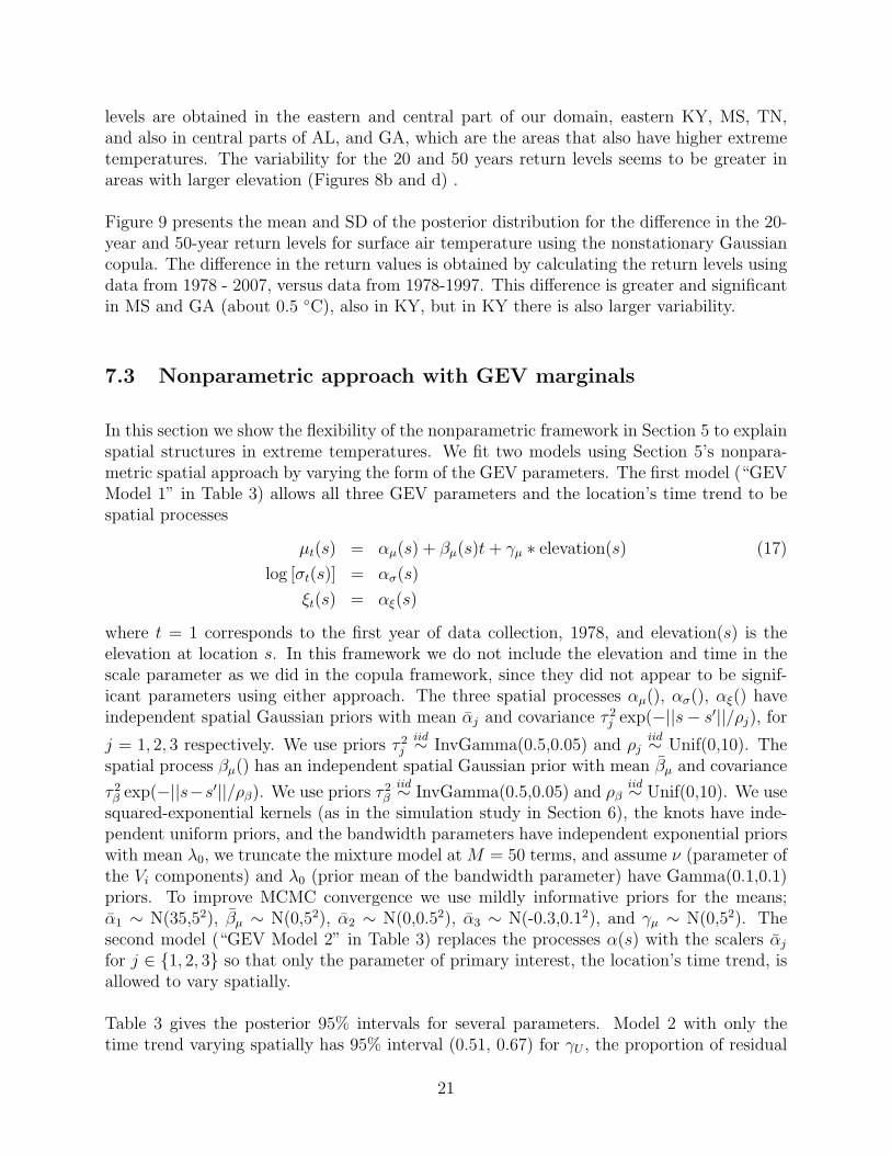
7.3 Nonparametric approach with GEV marginals
In this section we show the flexibility of the nonparametric framework in Section 5 to explainspatial structures in extreme temperatures. We fit two models using Section 5’s nonpara-metric spatial approach by varying the form of the GEV parameters. The first model (“GEVModel 1” in Table 3) allows all three GEV parameters and the location’s time trend to bespatial processes
µt(s) = αµ(s) + βµ(s)t+ γµ ∗ elevation(s) (17)
log [σt(s)] = ασ(s)
ξt(s) = αξ(s)
where t = 1 corresponds to the first year of data collection, 1978, and elevation(s) is theelevation at location s. In this framework we do not include the elevation and time in thescale parameter as we did in the copula framework, since they did not appear to be signif-icant parameters using either approach. The three spatial processes αµ(), ασ(), αξ() haveindependent spatial Gaussian priors with mean αj and covariance τ 2
j exp(−||s− s′||/ρj), for
j = 1, 2, 3 respectively. We use priors τ 2j
iid∼ InvGamma(0.5,0.05) and ρjiid∼ Unif(0,10). The
spatial process βµ() has an independent spatial Gaussian prior with mean βµ and covariance
τ 2β exp(−||s−s′||/ρβ). We use priors τ 2
βiid∼ InvGamma(0.5,0.05) and ρβ
iid∼ Unif(0,10). We usesquared-exponential kernels (as in the simulation study in Section 6), the knots have inde-pendent uniform priors, and the bandwidth parameters have independent exponential priorswith mean λ0, we truncate the mixture model at M = 50 terms, and assume ν (parameter ofthe Vi components) and λ0 (prior mean of the bandwidth parameter) have Gamma(0.1,0.1)priors. To improve MCMC convergence we use mildly informative priors for the means;α1 ∼ N(35,52), βµ ∼ N(0,52), α2 ∼ N(0,0.52), α3 ∼ N(-0.3,0.12), and γµ ∼ N(0,52). Thesecond model (“GEV Model 2” in Table 3) replaces the processes α(s) with the scalers αj
for j ∈ {1, 2, 3} so that only the parameter of primary interest, the location’s time trend, isallowed to vary spatially.
Table 3 gives the posterior 95% intervals for several parameters. Model 2 with only thetime trend varying spatially has 95% interval (0.51, 0.67) for γU , the proportion of residual
21
Table 3: Posterior medians (95% intervals) for the yearly maximum temperature data. Thefirst model has spatially varying coefficients for all GEV parameters, the second model allowsonly the location’s time trend to vary spatially.
Parameter GEV Model 1 GEV Model 2Stick-breaking parameter (γU) 0.03 ( 0.02, 0.07) 0.60 ( 0.51, 0.67)Mean location, intercept (α1) 36.8 ( 34.1, 39.0) 36.9 ( 36.9, 37.2)Mean location, time trend (βµ) 0.01 (-0.14, 0.13) -0.01 (-0.19, 0.16)Mean log scale (α2) -0.10 (-0.49, 0.27) 0.29 ( 0.22, 0.37)Mean shape (α3) -0.20 (-0.39, -0.03) -0.06 (-0.09, -0.02)Mean location, elevation (γµ) -0.63 (-1.00, -0.28) -0.03 (-0.21, 0.18)SD location, intercept (τ1) 2.02 ( 1.37, 2.98) –SD location, time trend (τβ) 0.10 ( 0.08, 0.13) 0.13 ( 0.10, 0.17)SD log scale (τ2) 0.28 ( 0.18, 0.50) –SD shape (τ3) 0.28 ( 0.18, 0.44) –
variance attributed to spatial process. Model 1 allows all of the GEV parameters to varyspatially, which absorbs most of the spatial trend leaving in Model 1 leaving 95% interval(0.02, 0.07) for γU . These models also give different estimates of the bandwidths (Figure10), the spatial variability in the bandwidth parameter explains the lack of stationarity inthe residuals after accounting for the spatially varying coefficients in the GEV parameters.In Model 2, there is more spatial variability in the bandwidth parameter, this is expected,since there is more spatial dependence left to explain in this model that has a simpler spatialstructure for the GEV parameters. Figure 10 plots the posterior mean and standard deviationof the spatially-varying time trend βµ(s) for the two models. The results are similar, thoughthe spatial patterns are more heterogeneous for Model 1 than Model 2, there is an increasingtrend in central AL and eastern MS, and a decreasing trend in central TN and KY, andparts of FL.
We obtained 20-year return levels using Models 1 and 2. In Figure 11, we plot the mean andSD of the posterior distribution for the 20-year return levels, with the location parameterat the final time-point. The spatial patterns obtained are very similar to the ones for themean extreme temperature values in Figure 4a. However, as expected, for the sample meanof extreme temperatures we have a smoother surface. Using Model 1, the 20-year returnlevels are about 2 ◦C greater than the sample mean for the extreme temperature values, thesame result was obtained using the spatial nonstationary Gaussian copula framework. The20-year return levels are about 4 ◦C greater using Model 2. The maximum values for thereturn levels are obtained in the eastern part of our domain, eastern KY, MS, TN, and alsoin central part of AL, and western part of GA, which are the areas with higher temperatures.However, in Model 1, since we have more parameters to estimate, there is larger uncertaintyin the estimated return levels than in Model 2. With Model 2 we have larger uncertaintyin areas with higher elevation (as with the copula approach), due probably to the fact thatthe role of elevation is explained better in Model 1 that has a spatially varying coefficient
22
for the location’s intercept.
8 Discussion
In this work we study the spatial structure of extreme temperature values. We introducemodelling frameworks that offer flexible approaches to characterize complex spatial patternsand explain potential nonstationarity in the extremes. In particular, we present a novelDirichlet-type mixture nonparametric approach that has GEV marginal distributions, butalso allows for residual correlation, avoiding the matrix inversion that is needed in the spatialcopula methods. This type of nonparametric framework offers a lot of flexibility, sincecomplex spatial models for the GEV parameters can be avoided by putting some relativelysimple structure in the residual component. We also present extensions of copula frameworksusing Dirichlet type of mixtures. An advantange of the formulation presented in this paperusing nonparametric models is that many of the tools developed for Dirichlet processes canbe applied with some modifications.
Multivariate extensions of the nonparametric spatial approaches presented here can be easilyadopted to model simultaneously maximum and minimum extreme temperature values orother extreme weather variables, using, for instance the nonparametric spatial frameworkproposed by Fuentes and Reich (2008). They could also easily be applied to spatial dailydata with Generalized Pareto marginal distributions.
References
An, Q., Wang, C., Shterev, I., Wang, E., Carin, L, and Dunson, D. (2009). Hierarchicalkernel stick-breaking process for multi-task image analysis. International Conference
on Machine Learning (ICML), to appear.
Buishand, D.H.L., and Zhou, C. (2008). On spatial extremes: with application to a rainfallproblem. Annals of Applied Probability, 2, 624-642.
Climate Change Science Program (CCSP) (2008). Weather and Climate Extremes in aChanging Climate Regions of Focus: North America, Hawaii, Caribbean, and U.S.Pacific Islands. U.S. goverments CCSP.
Coles, S.G. (1993). Regional modeling of extreme storms via max-stable processes. Journal
of the Royal Statistical Society, B, 55, 797-816.
Coles, S.G., and Tawn, J.A. (1996). Modelling extremes of the areal rainfall process.Journal of the Royal Statistical Society, B, 58, 329-347.
23
Cooley, D. D. Nychka, and P. Naveau. (2007) Bayesian Spatial Modeling of ExtremePrecipitation Return Levels. Journal of the American Statistical Association, 102,824-840.
Cooley, D., Naveau, P., and Davis, R. (2008). Dependence and spatial prediction in max-stable random fields. University of Colorado.
Dai, A., T.M.L. Wigley, B. A. Boville, J.T. Kiehl, and L.E. Buja. (2001). Climates of the20th and 21st centuries simulated by the NCAR climate system model. Journal of
Climate, 14, 485-519.
Davison, A.C., Smith, R.L. (1990). Models for exceedances over high thresholds. Journal
of the Royal Statistical Society, B, 15, 393-442.
Doksum, K. (1974). Tailfree and Neutral Random Probabilities and Their Posterior Dis-tributions. The Annals of Probability, 2, 183-201
Dunson, D.B. and J. H. Park. (2008). Kernel stick-breaking processes. Biometrika, 95,307-323.
Eastoe, E.F. (2009). A hierarchical model for non-stationary multivariate extremes: a casestudy of surface-level ozone and NOx data in the UK. To appear in Environmetrics.
Eastoe, E.F., Tawn, J.A. (2009). Modelling non-stationary extremes with application tosurface-level ozone. To appear in Journal of the Royal Statistical Society, C.
Ferguson TS (1973). A Bayesian analysis of some nonparametric problems. The Annals of
Statistics, 1, 209-230.
Fisher, R. A., and Tippett, L.H.C. (1928). Limiting forms of the frequency distributionof the largest or smallest member of a sample. Proc. Cambridge Philos. Soc., 24,180-190.
Fuentes, M. (2001). A High Frequency Kriging for Nonstationary Environmental Processes.Environmetrics, bf 12, 1-15.
Fuentes, M., and Reich, B. (2008). Multivariate Spatial Nonparametric Modelling viaKernel Processes Mixing. Mimeo Series #2622 Statistics Department, NCSU.
http://www.stat.ncsu.edu/library/mimeo.html.
Galanbos, J. (1987). The asymptotic theory of extreme order statistics. Second edition.Krieger, Melbourne, Fl.
Gelfand A.E., Kottas A., and MacEachern S.N. (2005). Bayesian Nonparametric SpatialModeling with Dirichlet Process Mixing. Journal of the American Statistical Associa-
tion, 100, 1021-1035.
Griffin J.E., and Steel, M.F.J. (2006) Order-based dependent Dirichlet processes. Journal
of the American Statistical Association, 101, 179-194
24
Joe, H. (1997). Multivariate models and dependence concepts, London: Chapman & Hall.
Kharin, V. and Zwiers, F. (2005). Estimating extremes in transient climate change simu-lations. Journal of Climate, 18, 1156-1173.
Mitchell, J.F.B., S. Manabe,V. Meleshko and T. Tokioka. (1990). Equilibrium climatechange and its implications for the future. In Climate Change. The IPCC ScientificAssessment. Contribution of Working Group 1 to the first assessment report of theIntergovernmental Panel on Climate Change, [Houghton, J. L, G. J. Jenkins and J.J. Ephraums (eds)], Cambridge University Press, Cambridge, pp. 137-164. Mitchell,J.F.B., T.C. Johns, J.M. Gregory and S.F.B. Tett,
Nasri-Roudsari, D. (1996). Extreme value theory of generalized order statistics Journal of
Statistical Planning and Inference, 55, 281-297.
Nelsen, R. (1999). An introduction to copulas, New York: Springer-Verlag.
Papaspiliopoulos O., and Roberts, G. (2008). Retrospective MCMC for Dirichlet processhierarchical models. Biometrika, 95, 169-186.
Parmesan, C., Root, T.L., and Willing, M.R. (2000). Bulletin of the American Meteorolog-
ical Society, 81, 443-450.
Pickands, J. (1981). Multivariate extreme value distributions, Proceedings of the 43rdSession ISI, Buenos Aires, 859-878.
Reich B.J., Fuentes M (2007). A multivariate semiparametric Bayesian spatial modelingframework for hurricane surface wind fields. Annals of Applied Statistics, 1 249-264.
Sang, H. and Gelfand, A.E. (2009). Hierarchical Modeling for Extreme Values Observedover space and time, Environmental and Ecological Statistics (forthcoming)
Stefano, D., McNeil, A. (2004). The t copula and related copulas. Tech. report, Departmentof Mathematics, Federal Institute of Technology, ETH Zentrum, Zurich.
Schlather, M. (2002). Models for stationary max-stable random fields. Extremes, 5, 33-44.
Schlather, M., and Tawn, J.A. (2003). A dependence measure for multivariate and spatialextreme values: properties and inference. Biometrika, 90, 139-156.
Smith, R.L. (1990). Max-stable processes and spatial extremes. Unpublished manuscript.Tech. report at University of North Carolina, Chapel Hill.
Tiago de Oliveira, J. (1975). Bivariate and multivariate extremal distribution. Statistical
distributions in scientific work, 1, 355-361. G. Patil et al., Dr. Reidel Publ. Co.
Vliet, A.J.H. van; Leemans, R. (2006) Rapid species responses to changes in climate re-quire stringent climate protection targets In: Avoiding dangerous climate change /Schellnhuber, H.J., Cramer, W., Nakicinovic, N., Wigley, T., Yohe, G. Cambridge :Cambridge University Press, 135 - 143.
25
Zhang, J., Craigmile, P.F., and Cressie, N. (2008). Loss Function Approaches to Predict aSpatial Quantile and Its Exceedance Region. Technometrics, 50 (2), 216-227.
Yonetani, T. and H.B. Gordon. (2001). Simulated changes in the frequency of extremes andregional features of seasonal/annual temperature and precipitation when atmosphericCO2 is doubled. Journal of Climate, 14, 1765-1779.
26
9 Appendix: Computing details
9.1 Spatial Gaussian copula
We assume that the annual maximum temperature at location si follows a GEV distributiongiven in (2) with location parameter µ(si), scale parameter σ(si) and shape parameter ξ(si),i = 1, . . . ,m. We denote the annual max temperature in year j at location si by Yj(si),i = 1, . . . ,m, and j = 1, . . . , n. Using a Gaussian nonstationary correlation matrix, thelikelihood is obtained by differentiating the cdf in (6), and is given byL(µ,σ, ξ, ρ|y(s1), . . .y(sm)) =
(
m∏
i=1
n∏
j=1
gsi(yj(si))
)
|Σ|−n/2 exp
{
−1
2
n∑
j=1
cTj
(
Σ−1 − Im)
cj
}
, (18)
where Im is an m×m identity matrix,
cTj =
[
Φ−1Gs1(yj(s1)), . . . ,Φ
−1Gsm(yj(sm))
]
, j = 1, . . . , n, (19)
and gsiandGsi
are the GEV pdf and cdf. Here µ = [µ(s1), . . . , µ(sm)]T , σ = [σ(s1), . . . , σ(sm)]T ,ξ = [ξ(s1), . . . , ξ(sm)]T , and y(si) = [y1(si), . . . , yn(si)]
T , i = 1, . . . ,m.
9.2 Nonparametric method
Joint analysis of the GEV location, shape, and scale parameters and the latent spatialcorrelation parameters requires computing the likelihood of the observations Yt(s). The dataare conditionally independent given the latent spatial parameters Ut(s). Changing variablesfrom the pure error component Wt(s) to the observations Yt(s) gives the conditional jointlikelihood
∏
s
∏
t
p (Yt(s)|Ut(s)) =∏
s
∏
t
fs,t (Yt(s)) k(Wt(s)|γW )/f(Zt(s)) (20)
where fs,t is the GEV density with location µt(s), scale σt(s), and shape ξt(s), k(Wt(s)|γW )is the Gamma(γW ,1) density, and f(Zt(s)) is the Frechet density.
The parameters in µt(s), σt(s), and ξt(s) are updated using Metropolis sampling. Their fullconditionals are the product of the likelihood in (20) and their Gaussian priors. Gaussiancandidate distributions are tuned to give acceptance rate near 0.4. Hyperparameters δjand τ 2
j have conjugate Gaussian and inverse gamma full conditionals, respectively, and areupdated using Gibbs sampling. The algorithm for updating the latent spatial parametersUt(s) and all other parameters in the spatial stick-breaking model are given in Reich andFuentes (2007). For all analyses we generate 25,000 MCMC samples and discard the first10,000 as burn-in. Convergence is monitored using trace plots of the deviance and severalrepresentative parameters.
27
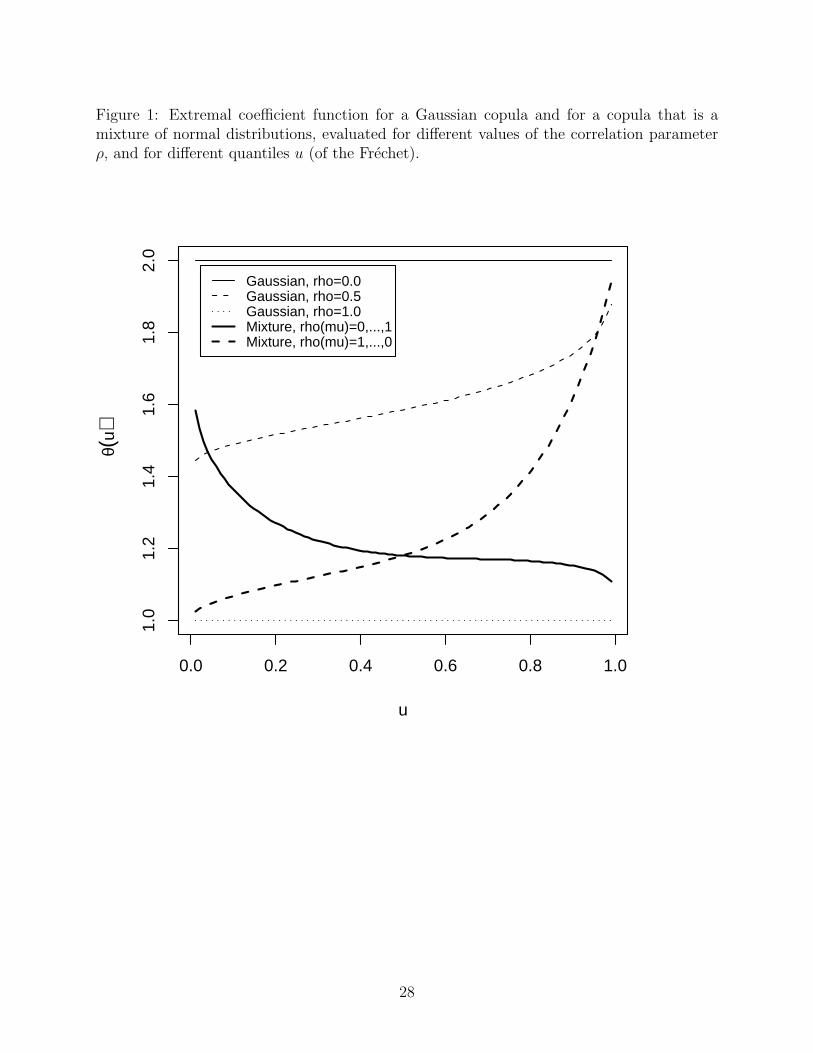
Figure 1: Extremal coefficient function for a Gaussian copula and for a copula that is amixture of normal distributions, evaluated for different values of the correlation parameterρ, and for different quantiles u (of the Frechet).
0.0 0.2 0.4 0.6 0.8 1.0
1.0
1.2
1.4
1.6
1.8
2.0
u
θ(u)
Gaussian, rho=0.0Gaussian, rho=0.5Gaussian, rho=1.0Mixture, rho(mu)=0,...,1Mixture, rho(mu)=1,...,0
28
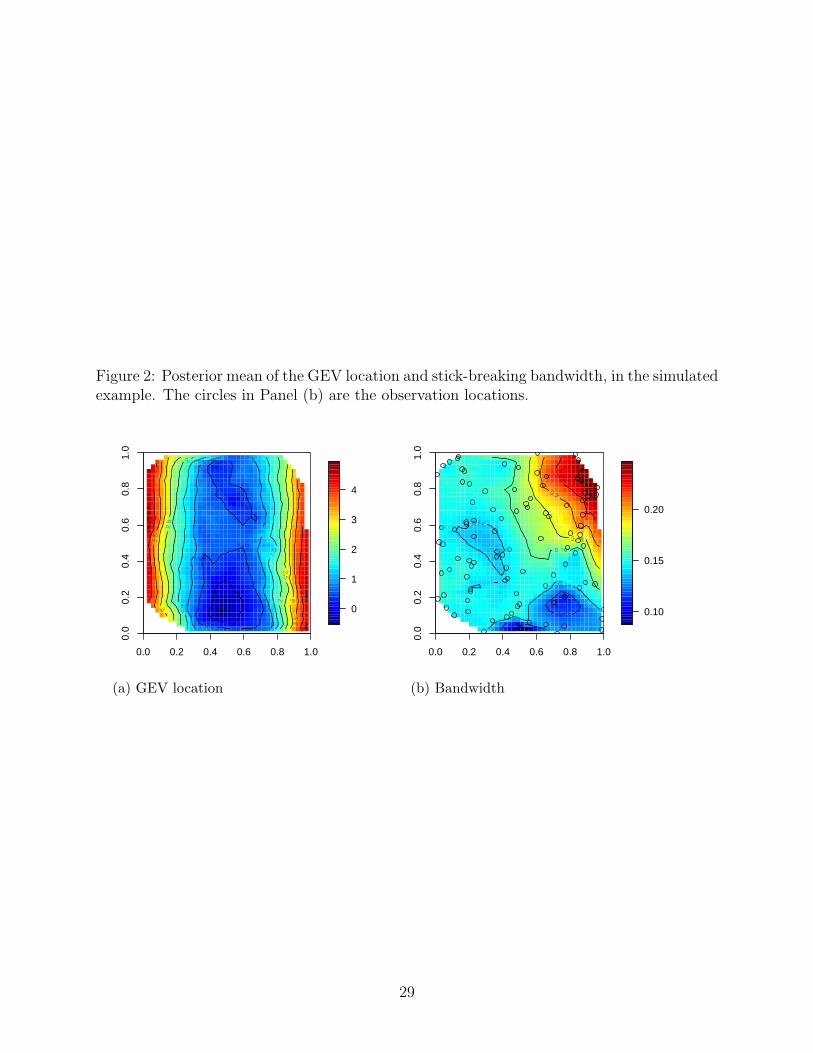
Figure 2: Posterior mean of the GEV location and stick-breaking bandwidth, in the simulatedexample. The circles in Panel (b) are the observation locations.
0.0 0.2 0.4 0.6 0.8 1.0
0.0
0.2
0.4
0.6
0.8
1.0
0
1
2
3
4
0.0 0.2 0.4 0.6 0.8 1.0
0.0
0.2
0.4
0.6
0.8
1.0
0.10
0.15
0.20
(a) GEV location (b) Bandwidth
29
Figure 3: The change in 20-year return values for daily maximum surface air temperature(◦C) simulated in a global coupled atmosphere-ocean model (CGCM1) in 2080 to 2100relative to the reference period 1975 to 1995 (graph from IPCC third report). Contourinterval is 4◦C. Zero line is omitted.
30
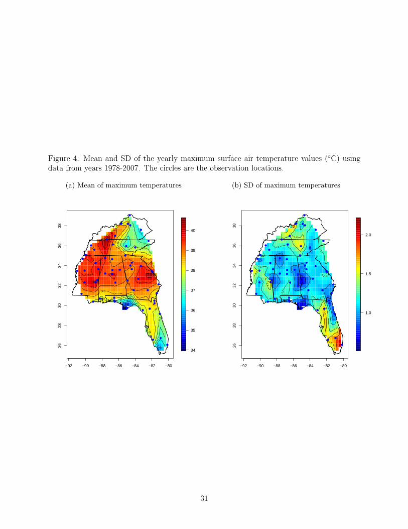
Figure 4: Mean and SD of the yearly maximum surface air temperature values (◦C) usingdata from years 1978-2007. The circles are the observation locations.
−92 −90 −88 −86 −84 −82 −80
2628
3032
3436
38
34
35
36
37
38
39
40
35.5
36
36.5
36.5
37
37
37
37
37.5
37.5
37.
5
38 38
38
38
38
38
38.5
38.5
39
39
39.5
39.5
39.5
39.5
39.5
40
40
−92 −90 −88 −86 −84 −82 −80
2628
3032
3436
38
1.0
1.5
2.0
0.8
0.8
1
1
1
1 1
1
1
1
1.2
1.2
1.2
1.2
1.2
1.2
1.2
1.4
1.4
1.4
1.4
1.6
1.6
1.8
(a) Mean of maximum temperatures (b) SD of maximum temperatures
31
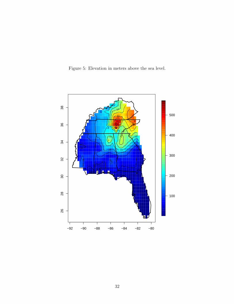
Figure 5: Elevation in meters above the sea level.
−92 −90 −88 −86 −84 −82 −80
2628
3032
3436
38
100
200
300
400
500
50
50
50
100
100
100
150 200
250 250
300
300
350
400
400
450
32
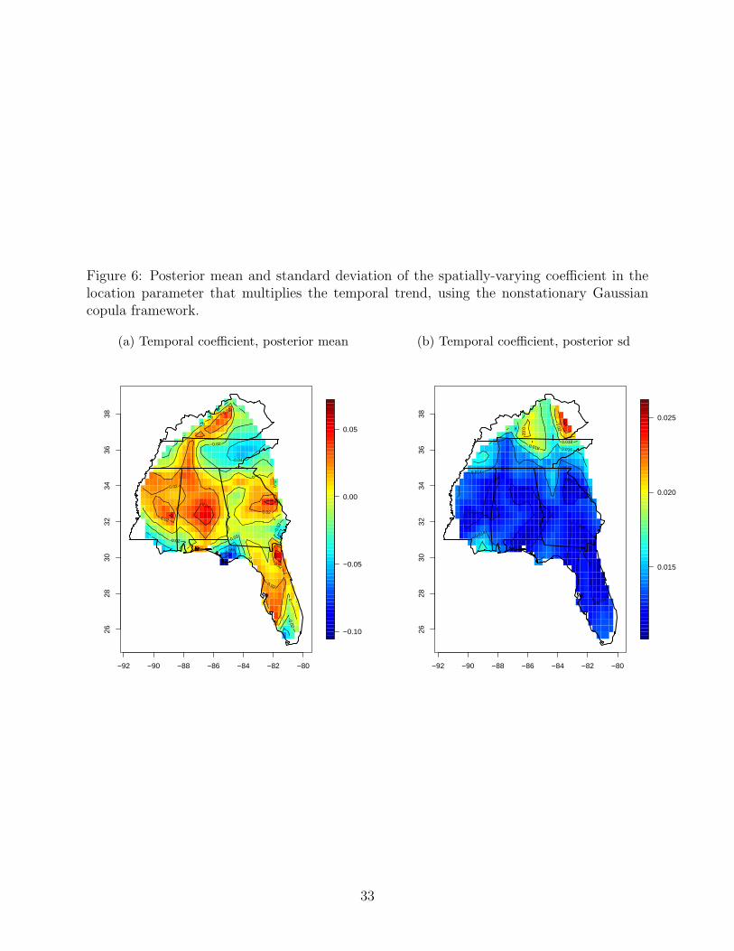
Figure 6: Posterior mean and standard deviation of the spatially-varying coefficient in thelocation parameter that multiplies the temporal trend, using the nonstationary Gaussiancopula framework.
−92 −90 −88 −86 −84 −82 −80
2628
3032
3436
38
−0.10
−0.05
0.00
0.05
−0.06
−0.04
−0.02
−0.02
−0.02
−0.
02
−0.02
0
0
0
0
0
0
0
0
0.02
0.02
0.02
0.02
0.02
0.02
0.04
−92 −90 −88 −86 −84 −82 −80
2628
3032
3436
38
0.015
0.020
0.025
0.012
0.012
0.012
0.012
0.012
0.014
0.014
0.016 0.018
0.018
0.02
0.02
(a) Temporal coefficient, posterior mean (b) Temporal coefficient, posterior sd
33
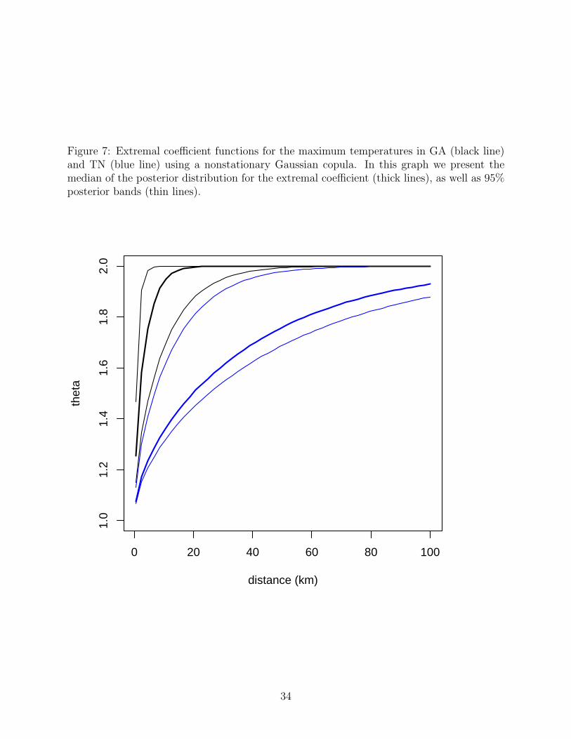
Figure 7: Extremal coefficient functions for the maximum temperatures in GA (black line)and TN (blue line) using a nonstationary Gaussian copula. In this graph we present themedian of the posterior distribution for the extremal coefficient (thick lines), as well as 95%posterior bands (thin lines).
0 20 40 60 80 100
1.0
1.2
1.4
1.6
1.8
2.0
distance (km)
thet
a
34
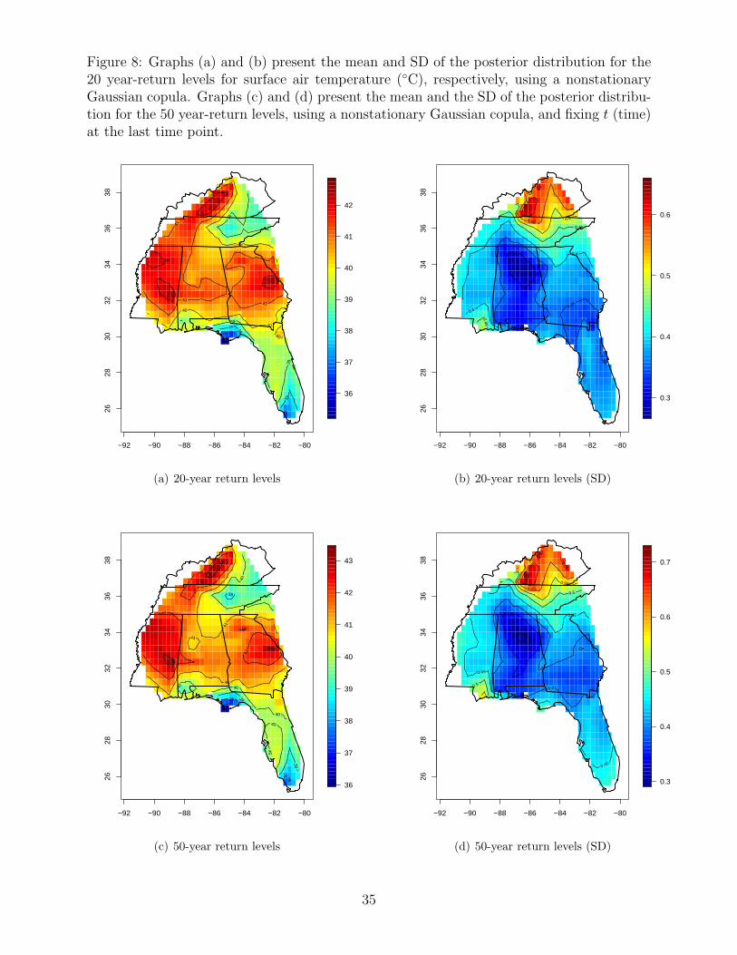
Figure 8: Graphs (a) and (b) present the mean and SD of the posterior distribution for the20 year-return levels for surface air temperature (◦C), respectively, using a nonstationaryGaussian copula. Graphs (c) and (d) present the mean and the SD of the posterior distribu-tion for the 50 year-return levels, using a nonstationary Gaussian copula, and fixing t (time)at the last time point.
−92 −90 −88 −86 −84 −82 −80
2628
3032
3436
38
36
37
38
39
40
41
42
37
38
38
39
39
39
40
40
40
40
41
41
41
42
42
42
42
(a) 20-year return levels
−92 −90 −88 −86 −84 −82 −80
2628
3032
3436
38
0.3
0.4
0.5
0.6
0.3
0.35
0.35
0.35
0.35
0.4
0.4
0.45
0.45
0.5 0.55
0.6
(b) 20-year return levels (SD)
−92 −90 −88 −86 −84 −82 −80
2628
3032
3436
38
36
37
38
39
40
41
42
43
38
38
39
39
39
40 40
40
40
40
40
41
41
41
42
42
42
42
43
43
(c) 50-year return levels
−92 −90 −88 −86 −84 −82 −80
2628
3032
3436
38
0.3
0.4
0.5
0.6
0.7
0.3
0.35
0.4 0.4
0.45
0.45
0.45
0.5
0.5
0.55 0.6
0.6
5
0.6
5
0.65
(d) 50-year return levels (SD)
35
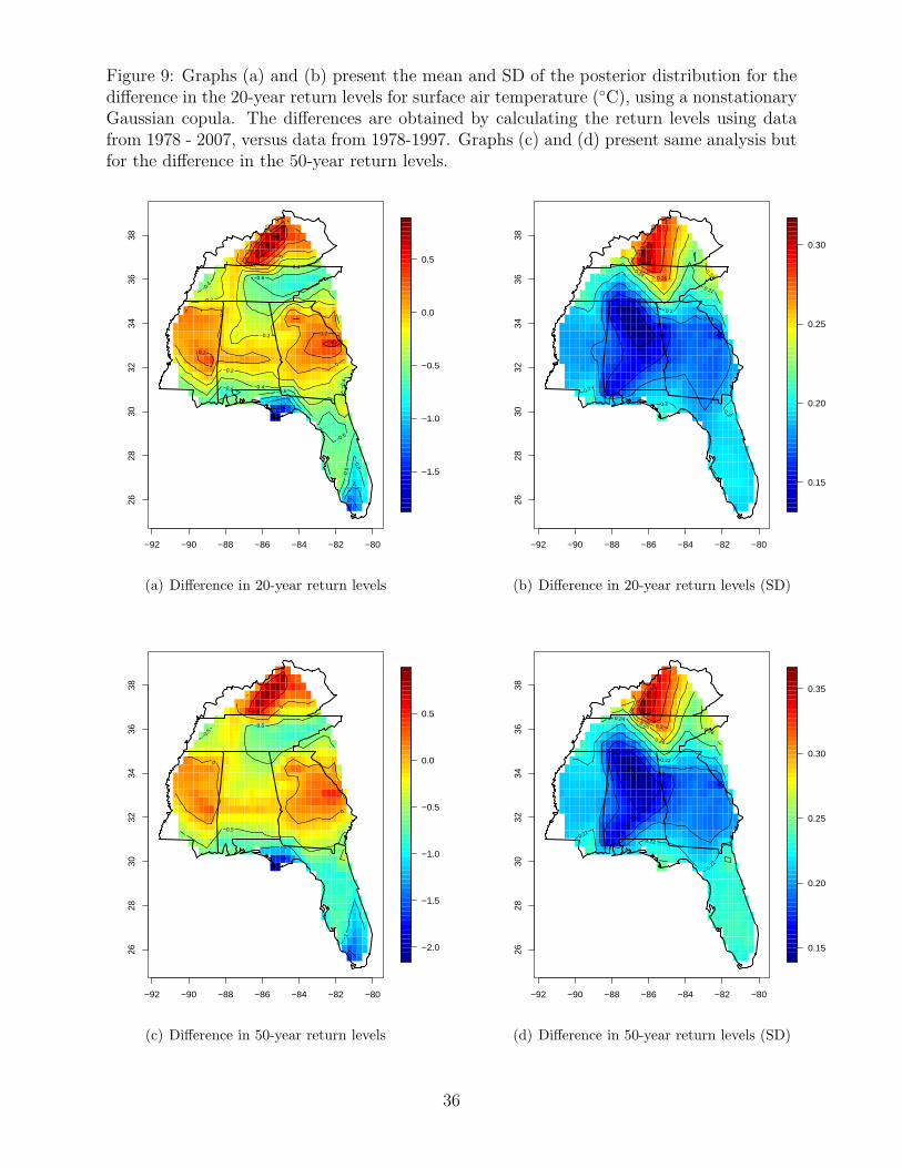
Figure 9: Graphs (a) and (b) present the mean and SD of the posterior distribution for thedifference in the 20-year return levels for surface air temperature (◦C), using a nonstationaryGaussian copula. The differences are obtained by calculating the return levels using datafrom 1978 - 2007, versus data from 1978-1997. Graphs (c) and (d) present same analysis butfor the difference in the 50-year return levels.
−92 −90 −88 −86 −84 −82 −80
2628
3032
3436
38
−1.5
−1.0
−0.5
0.0
0.5
−1.2
−1 −0.8
−0.6
−0.6
−0.6
−0.6
−0.
6
−0.4
−0.4
−0.4
−0.
4
−0.2
−0.2
−0.2
0
0
0
0.2
0.2
0.2
0.4
0.4
0.6
(a) Difference in 20-year return levels
−92 −90 −88 −86 −84 −82 −80
2628
3032
3436
38
0.15
0.20
0.25
0.30
0.14
0.16
0.18
0.2
0.2
0.2
0.2
0.22
0.24 0.24 0.26
0.2
8
(b) Difference in 20-year return levels (SD)
−92 −90 −88 −86 −84 −82 −80
2628
3032
3436
38
−2.0
−1.5
−1.0
−0.5
0.0
0.5
−1.5
−1
−1
−0.5
−0.
5
−0.5
0
0
0
0.5
(c) Difference in 50-year return levels
−92 −90 −88 −86 −84 −82 −80
2628
3032
3436
38
0.15
0.20
0.25
0.30
0.35
0.16
0.18
0.2
0.22
0.22
0.22
0.2
2 0.24
0.26
0.26
0.28 0.3
0.32
0.3
4
(d) Difference in 50-year return levels (SD)
36
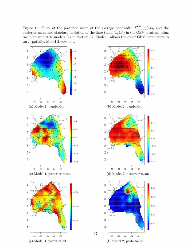
Figure 10: Plots of the posterior mean of the average bandwidth∑M
i=1 pi(s)λi and theposterior mean and standard deviation of the time trend (βµ(s)) in the GEV location, usingtwo nonparametric models (as in Section 5). Model 1 allows the other GEV parameters tovary spatially, Model 2 does not.
−90 −88 −86 −84 −82
26
28
30
32
34
36
38
4.1
4.2
4.3
4.4
4.5
4.6
4.7
−90 −88 −86 −84 −82
26
28
30
32
34
36
38
1.5
2.0
2.5
3.0
3.5
4.0
(a) Model 1, bandwidth (b) Model 2, bandwidth
−90 −88 −86 −84 −82
26
28
30
32
34
36
38
−0.06
−0.04
−0.02
0.00
0.02
0.04
−90 −88 −86 −84 −82
26
28
30
32
34
36
38
−0.15
−0.10
−0.05
0.00
0.05
0.10
(c) Model 1, posterior mean (d) Model 2, posterior mean
−90 −88 −86 −84 −82
26
28
30
32
34
36
38
0.010
0.015
0.020
−90 −88 −86 −84 −82
26
28
30
32
34
36
38
0.014
0.016
0.018
0.020
0.022
(e) Model 1, posterior sd (f) Model 2, posterior sd
37
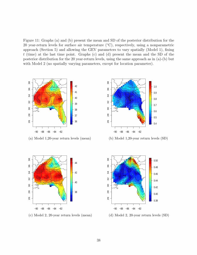
Figure 11: Graphs (a) and (b) present the mean and SD of the posterior distribution for the20 year-return levels for surface air temperature (◦C), respectively, using a nonparametricapproach (Section 5) and allowing the GEV parameters to vary spatially (Model 1), fixingt (time) at the last time point. Graphs (c) and (d) present the mean and the SD of theposterior distribution for the 20 year-return levels, using the same approach as in (a)-(b) butwith Model 2 (no spatially varying parameters, except for location parameter).
−90 −88 −86 −84 −82
26
28
30
32
34
36
38
36
37
38
39
40
41
42
−90 −88 −86 −84 −82
26
28
30
32
34
36
38
0.4
0.5
0.6
0.7
0.8
0.9
1.0
(a) Model 1,20-year return levels (mean) (b) Model 1,20-year return levels (SD)
−90 −88 −86 −84 −82
26
28
30
32
34
36
38
38
40
42
44
−90 −88 −86 −84 −82
26
28
30
32
34
36
38
0.38
0.40
0.42
0.44
0.46
0.48
0.50
(c) Model 2, 20-year return levels (mean) (d) Model 2, 20-year return levels (SD)
38