Nonlinear response function for time-domain and frequency-domain four-wave mixing

Vol. 3, No. 4/April 1986/J. Opt. Soc. Am. B 595

Nonlinear response function for time-domain andfrequency-domain four-wave mixing

Shaul Mukamel and Roger F. Loring

Department of Chemistry, The University of Rochester, River Station, Rochester, New York 14627

Received September 20, 1985; accepted November 19, 1985

A unified theory of time-domain and frequency-domain four-wave mixing processes, which is based on the nonlinearresponse function R(t 3 , t 2, t), is developed. The response function is expressed in terms of the four-pointcorrelation function of the dipole operator F(r 1 , T2, T3, 4) and is evaluated explicitly for a stochastic model of linebroadening that holds for any correlation time of the bath. Our results interpolate between the fast-modulationlimit, in which the optical Bloch equations are valid, and the static limit of inhomogeneous line broadening. As anexample of the relationship between time-domain and frequency-domain four-wave mixing, we compare thecapabilities of steady-state and transient coherent anti-Stokes Raman spectroscopy experiments to probe thevibrational dynamics in ground and excited electronic states.

1. INTRODUCTION

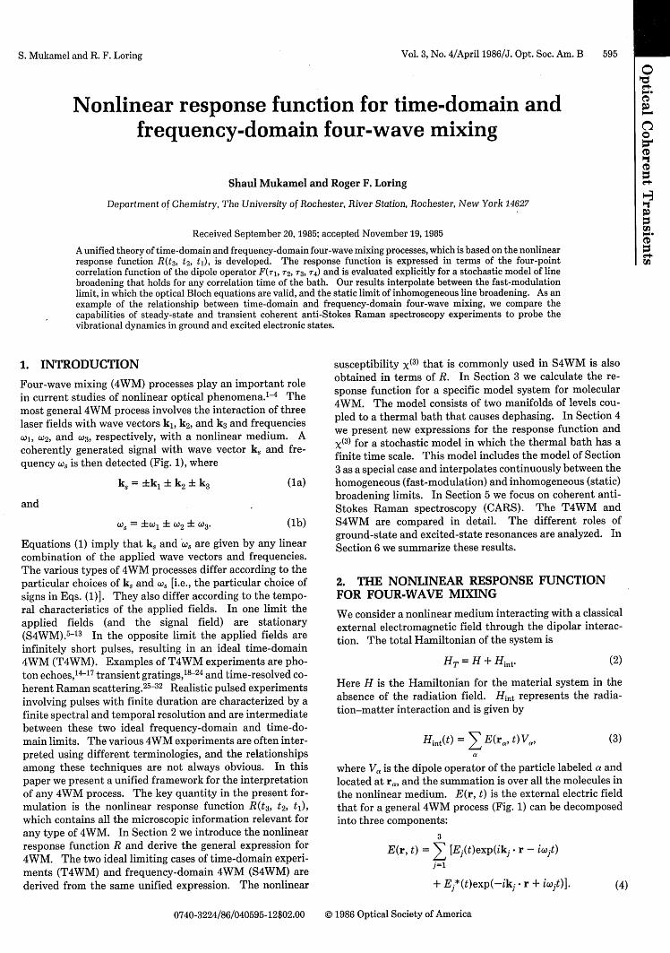
Four-wave mixing (4WM) processes play an important rolein current studies of nonlinear optical phenomena.l-4 Themost general 4WM process involves the interaction of threelaser fields with wave vectors kj, k2, and k3 and frequencies

°1, W2, and W3, respectively, with a nonlinear medium. Acoherently generated signal with wave vector k, and fre-quency co, is then detected (Fig. 1), where

k,= :+k k2 k3 (la)

and

°s = W@1 4- W2 W@3- (lb)Equations (1) imply that k, and wo are given by any linearcombination of the applied wave vectors and frequencies.The various types of 4WM processes differ according to theparticular choices of k, and w, [i.e., the particular choice ofsigns in Eqs. (1)]. They also differ according to the tempo-ral characteristics of the applied fields. In one limit theapplied fields (and the signal field) are stationary(S4WM).5-13 In the opposite limit the applied fields areinfinitely short pulses, resulting in an ideal time-domain4WM (T4WM). Examples of T4WM experiments are pho-ton echoes,'4 '7 transient gratings,'>24 and time-resolved co-herent Raman scattering.2 5-32 Realistic pulsed experimentsinvolving pulses with finite duration are characterized by afinite spectral and temporal resolution and are intermediatebetween these two ideal frequency-domain and time-do-main limits. The various 4WM experiments are often inter-preted using different terminologies, and the relationshipsamong these techniques are not always obvious. In thispaper we present a unified framework for the interpretationof any 4WM process. The key quantity in the present for-mulation is the nonlinear response function R(t 3 , t2 , t),which contains all the microscopic information relevant forany type of 4WM. In Section 2 we introduce the nonlinearresponse function R and derive the general expression for4WM. The two ideal limiting cases of time-domain experi-ments (T4WM) and frequency-domain 4WM (S4WM) arederived from the same unified expression. The nonlinear

susceptibility X(3 ) that is commonly used in S4WM is alsoobtained in terms of R. In Section 3 we calculate the re-sponse function for a specific model system for molecular4WM. The model consists of two manifolds of levels cou-pled to a thermal bath that causes dephasing. In Section 4we present new expressions for the response function andX(3) for a stochastic model in which the thermal bath has afinite time scale. This model includes the model of Section3 as a special case and interpolates continuously between thehomogeneous (fast-modulation) and inhomogeneous (static)broadening limits. In Section 5 we focus on coherent anti-Stokes Raman spectroscopy (CARS). The T4WM andS4WM are compared in detail. The different roles ofground-state and excited-state resonances are analyzed. InSection 6 we summarize these results.

2. THE NONLINEAR RESPONSE FUNCTIONFOR FOUR-WAVE MIXING

We consider a nonlinear medium interacting with a classicalexternal electromagnetic field through the dipolar interac-tion. The total Hamiltonian of the system is

HT = H + Hit (2)

Here H is the Hamiltonian for the material system in theabsence of the radiation field. Hint represents the radia-tion-matter interaction and is given by

Hint(t) = Z E(rac, t) V, (3)

where Va is the dipole operator of the particle labeled a andlocated at r, and the summation is over all the molecules inthe nonlinear medium. E(r, t) is the external electric fieldthat for a general 4WM process (Fig. 1) can be decomposedinto three components:

3

E(r, t) = E [Ej(t)exp(ikj- r - iwjt)j=1

+ Ej*(t)exp(-ikj- r + ijt)].

0740-3224/86/040595-12$02.00 © 1986 Optical Society of America

(4)

S. Mukamel and R. F. Loring

596 J. Opt. Soc. Am. B/Vol. 3, No. 4/April 1986

For a 4WM process we calculate p(t) perturbatively to third14, order in Lint. We then get

kS P(r, t) = (-i) 3dT 3 dr 2 dT, ((11 9(t T3)Ljnt(T3)

X -(T3 r2)Lint(r2)9(r 2 - T7)Lijt(7i)!p(-c))). (12)

Here the Green function g(T) is the formal solution of Eq. (8)in the absence of the electromagnetic field:

k3 17 3

Fig. 1. The general 4WM process. The coherent signal with wavevector k is generated by a nonlinear mixing of the applied fieldswith wave vectors k, k2 , and k3.

We shall now adopt a simple model in which the activenonlinear medium consists of noninteracting absorbers anda set of bath degrees of freedom that interact with the ab-sorbers but not with the electromagnetic field. In this casewe can focus on one absorber located at r and write

Hint(t) = E(r, t)V, (5)

where V is the dipole operator of that absorber.In order to calculate the 4WM signal, we start at t = -

and assume that the system is in thermal equilibrium withrespect to H (without the radiation field)

p(-) = exp(-fH)/Tr exp(-,3H), (6)

where 3 = (kT)-1. The system then evolves in time accord-ing to the Liouville equation

dp _ i[H, p] - int PI-dt

In Liouville-space notation,33

dp =- iLp -iLinPdt

For subsequent manipulations we shall also introduce theGreen function in the frequency domain:

(Cw) = -i dr exp(iwr)9(T) = -o o -L

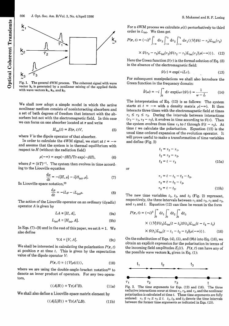
The interpretation of Eq. (12) is as follows: The systemstarts at t = - with a density matrix p(--). It theninteracts three times with the electromagnetic field at timesT1 < T2 < T3. During the intervals between interactions(722- rl, -3-T2), it evolves in time according to g(T). Thenthe system evolves from time 3 to t through (t - r3). Attime t we calculate the polarization. Equation (12) is theusual time-ordered expansion of the evolution operator. Itwill prove useful to make a transformation of time variablesand define (Fig. 2)

t = T2 -T1,

t2 = T3 T21

t3 = t - 3

or

l = t tl -t 2 t3,

T2 = t - t2 - t3,

T3 = t - t3.

The new time variables t, t2 , and t3 (Fig. 2) represent,respectively, the three intervals between rl and 2, 2 and 3,and 73 and t. Equation (12) can then be recast in the form

P(r, t) = (-i)3 dtL| dt2 - dt3

X ( ( g(OLint(t - 094~2)Lnt(t -t2 -tO)

(7)

(8)

The action of the Liouville operator on an ordinary (dyadic)operator A is given by

(9a)

(9b)

In Eqs. (7)-(9) and in the rest of this paper, we seth = 1. Wealso define

'VA -= [V, A]. (9c)

We shall be interested in calculating the polarization P(r, t)at position r at time t. This is given by the expectationvalue of the dipole operator V:

X Y(t)Lj(t - tl -t2- t3)jp(-)))- (16)

On the substitution of Eqs. (4), (5), and (9b) into Eq. (16), weobtain an explicit expression for the polarization in terms ofthe incoming field amplitudes E(t). P(r, t) can have any ofthe possible wave vectors k given in Eq. (1):

(10)

where we are using the double-angle-bracket notation3 3 todenote an inner product of operators. For any two opera-tors,

((AIB)) - Tr(AtB). (Ila)

We shall also define a Liouville-space matrix element by

((AILIB)) Tr(AtLB). (llb)

t1 t2 t3

40p * * *T1 T2 T3 tFig. 2. The time arguments for Eqs. (12) and (16). The threeradiative interactions occur at times ri, T2, and T3, and the nonlinearpolarization is calculated at time t. These time arguments are fullyordered: T T2 T3 < t. t, t 2, and t3 denote the time intervalsbetween the former time arguments as indicated in Eqs. (15).

ft 9(T) - exp(-iLr). (13)

(14)

(15a)

LA - [H, A],

LintA -- [Hint, A].

(15b)

*w * < * * -


P(r, t) m ((J�p(t))),


P(r, t) = E exp(iks. r - it)P(k, t).k8,w,

Hereafter, we shall select a specific choice, namely,

k =k,+k2 +k3 (18a)and

W = W1 + 'W2 + 3- (18b)

Any other combination may be obtained from our final ex-pression by changing one (or more) kj and wj into -kj and-wj and Ej(t) into Ej*(t). Using Eqs. (4), (5), and (16)-(18),we then get

= .i: 3P~~k,, t) f-l 2 t 3 dt2 f° d

X R(t 3, t2 , tj)exp[i(wm + W, + wq)t3 + i(Wm + Wd)t 2 + tWmtll

X Em(t - tl - t2 - t3)En(t - t2- t3)Eq(t - t3). (19)

R(t 3 , t2, t) is the nonlinear response function, whichcontains all relevant microscopic information:

R(t3, t2, tl) ((V g(t3)V(t2)'rg(tl)VI p(-c))). (20)

The summation in Eq. (19) is over all 3! = 6 permutations ofthe indices m, n, and q with the numbers 1, 2, and 3. Alter-natively, we may define the response function in the fre-quency domain by performing a Fourier transform ofR(t 3 , t2 , t1):

R(WmW + n + )q, C + on", WmY) (-i)3 f dt3 f dt2 f dt,

X exp[i(c, + con + Wq)t3 + i(Wrm + cvn)t2 + LWmtl]

x R(t3, t2 t).

Equation (19) may then be rearranged in the form

P(k,, t) = I J dw'rn dco f d'qrmn q =1,2,3 - J-

XR(w'm+c'n+W'q, W'm +0',, W'm)Jm(('m)Jn(W'n)Jq(W'q)

X exp[i(m + n + q 0 m n w 'q)t], (22)

where

(com+Cn +Wq, m + Cn, Wm)

- ((V19(Wm + n + Wq)V*(rm + WnYVg(WmYV1P(- 2)

(23)

and

Jj (co'j)= (27r) J drEj(7)exp[i(w'j - wj)7], j = m, n, q

(24)

is the spectral density of the j field.Equations (19) and (20) or alternatively Eqs. (22)-(24)

provide the most general formal expression for any type of4WM process.' 2 The signal (field intensity) in the k, direc-tion is obtained by substituting P(k8, t) as a source into theMaxwell equations and solving for the signal field. Whenthe incident fields do not vary substantially during the pro-

(17) cess, the signal is simply proportional to the absolute squareof P(ks, t). We thus have for the 4WM signal in the k,direction at time t (apart from some numerical and geomet-rical factors):

S(ks, t) = IP(k,, t)l2. (25)

Equations (19) and (20) or (22)-(24) show that the nonlinearresponse function R(t 3, t2, ti) or its Fourier transform P?(wm+ n + Wq, Wm + Wn, Wm) contains the complete microscopicinformation relevant to the calculation of any 4WM signal.As indicated earlier, the various 4WM techniques differ bythe choice of k, and W, and by the temporal characteristics ofthe incoming fields E,(t), E2(t), and E3(t). A detailed analy-sis of the response function and the nonlinear signal will bemade in Sections 3-5 for two specific models. At this point,we shall consider the two limiting cases of ideal T4WM andS4WM. In an ideal time-domain 4WM (T4WM), the dura-tions of the incoming fields are infinitely short, i.e.,

Ej(r) = Eb(r - 7*),

E2(T) = E26(T - 2),

E3(T) = E36(T - 7*3), (26)

where T*1 <T*2< 7*3 Wefurtherdenotet, = T*2 -T*1, t2 =7*3 - T*2, and t3 = t- *3. On the substitution of Eqs. (26)into Eq. (19) we get

P8(k8, t) = EjE2E3 R(t3, t2, tj)exp[ijt, + i(Wj + cW2)t2+ i(W, + W2 + o.,3)t 3] (27)

and

S(k, t) = EjE2 E321R(t3, t2, t) 2

. (28)

The other extreme limit of 4WM is a stationary frequency-21) domain experiment (S4WM) in which the field amplitudes

E1(7), E2(T), and E3(r) are time independent. In this casewe have

Jj(w' ) = E16(c - ,),

J2(W/2) = E26(W'2 -(2),

J3 (W13) = E3 5(W13 - W3)

Using Eqs. (22) and (29), we get

P(kwe t) = x(3)(_tbi W1 i2s ivEEn b

where the nonlinear susceptibility (3) is given by

X(3 )(-W" W911 W2 Wd

= P(Wm + Con + qs OM + n m)-m,nq=1,2,3

The stationary signal [Eq. (25)] is given in this case by

S(ks) = IEjE2E32

1X(3 )(-W" W1, o 2 WA2.

(29)

(30)

(31)

(32)

3. A MOLECULAR MODEL FOR THENONLINEAR RESPONSE FUNCTION: THEOPTICAL BLOCH EQUATIONS

In order to gain a better insight into the significance of thenonlinear response function [Eq. (20) or (23)], we shall nowconsider a specific model system commonly used in molecu-



A, -

(01 ( ~ b(1)3

rjfOr,

(35)P(--) = Ia)P(a)(aj,a

Y d or, in Liouville-space notation,

(36)

(Os Ybwhere

P(a) = exp(-OElE exp(-flEa)-a

04

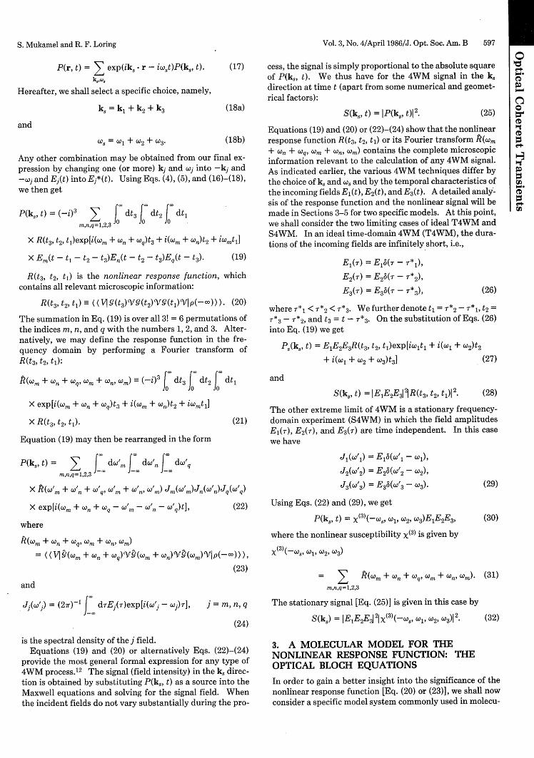
YaFig. 3. The molecular level scheme and laser frequencies for 4WM.Levels I a) and Ic ) are part of the ground-state vibrational manifold,whereas levels Ib) and Id) belong to an electronically excited mani-fold. y, is the inverse lifetime of level Iv). The electronic-dipoleoperator [Eq. (34)] couples vibronic states belonging to differentelectronic states.

lar 4WM. We consider a molecular level scheme for theabsorber consisting of a manifold of vibronic levels belong-ing to the ground electronic state denoted I a), I c), . . . , and amanifold of vibronic levels belonging to an excited electronicstate denoted Ib), Id), . . . (Fig. 3). The absorber is furthercoupled to a thermal bath, and the Hamiltonian for thenonlinear medium is

H = HS + HSB, (33a)

HS = E 0 I )(V2Y)( (33b)v=a,b,c,d .. .

HSB I v)HSB(QB) (vI (33c)v=a,b,c,d ...

Here ep is the energy and yv is the inverse lifetime of the I v)level. H is decomposed into a system Hamiltonian HS and asystem-bath Hamiltonian HSB which is taken to be diagonalin the system states I ). The bath coordinates are denotedQB. The electronic-dipole operator of the absorber couplesvibronic states belonging to different electronic states. Wethen have

V Z (Iaba) (bI + adla) (djab,c,d

+ cbI C) (b + Cdlc) (dl + H.c.), (34)

where the summation runs over the entire manifolds ofground and electronically excited states. The molecule istaken to be initially at thermal equilibrium in the ground-state manifold, i.e.,

(37)

In order to calculate the response function [Eq. (20)] we needthe matrix elements of the absorber's Green function [Eq.(13)]. Since our Hamiltonian H [Eqs. (33)] is diagonal in theabsorber states, we simply have

( (v'X'Ig(t)IvX) )s = ((vXJ9(t)IvX) )savv'5AA' (38a)

where

((vXIg(t)IvX))s = exp[-i,,\t - (1/2 )(y, + y)t]

X ( (vAjexp(-iLSB0) ) )5

v, = a, b, c, d . . , (38b)Xv- - (39)The action of the Liouville operator LSB on an operator A isgiven by

LSBA [HSB, A] (40)

The subscript s in Eqs. (38) indicates that the matrix ele-ment involves a partial trace over the system (absorber)degrees of freedom, and ((vX.G(t)IvX)), is still a Liouville-space operator in the bath degrees of freedom. In general,Eqs. (38) should be substituted into Eq. (20), and the result-ing expression should be averaged over the bath degrees offreedom. In this section, we shall adopt the Bloch equationsto account for the bath. In the absence of a radiation field,the Bloch equations for p, the density matrix averaged overthe bath degrees of freedom, are

d = (-iwA- P v, = a, b, c, d ...dt

where

p TrB(p)

and

rP = /2 (,, + 7Y + A

(41a)

(41b)

(41c)

The pure dephasing rate P",, is the only effect of the bath inthis approximation. The bath does not affect populations,i.e., F,, = 0. Typically, if v and belong to two differentelectronic states (e.g., v = ab), then the pure-dephasing rateis much larger than if they belong to the same electronicstate (e.g., vX = ac). The solution of Eq. (41a) is

PX(t) = ( vAL (t)Iv ) )P,,$O), (42a)

where the double brackets now denote a total trace (over thesystem and the bath), i.e.,

(42b)

The optical Bloch equations hold when the correlation timeof the bath is very short compared with the time scale of the

I a

l l


1)�(__M = �1 P(a)jaa)),

F I F

((vXI9(0jvX)) =TrB((V'\I9M1P1$),-


,1 0

/

0Co

. o

/

4o

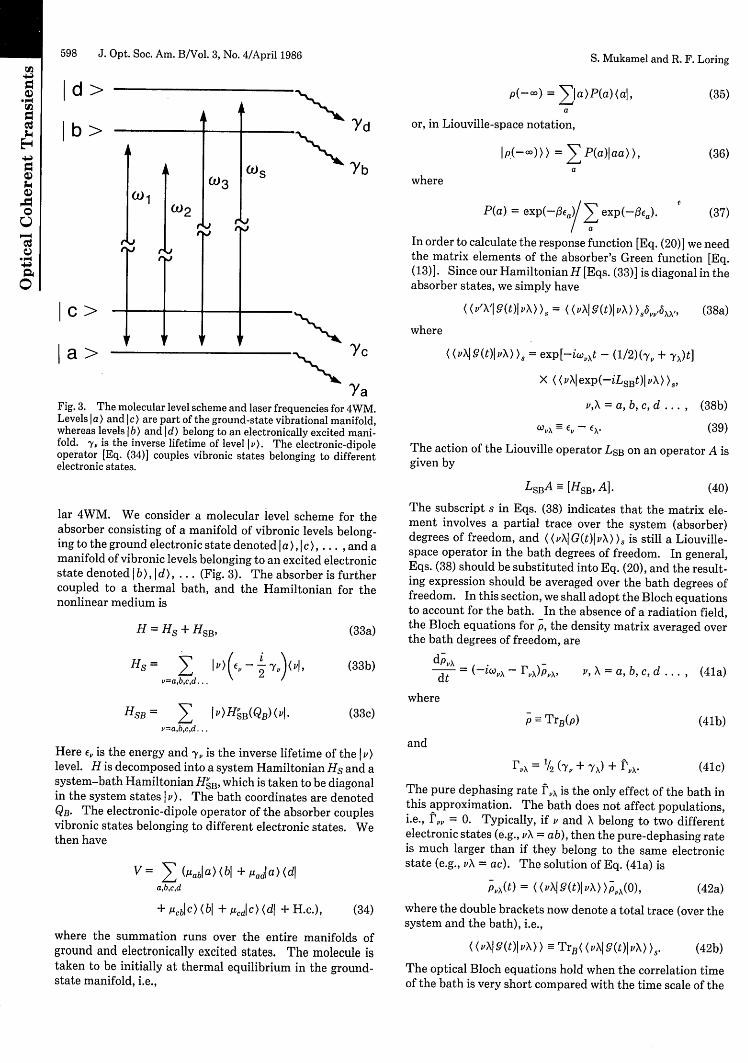
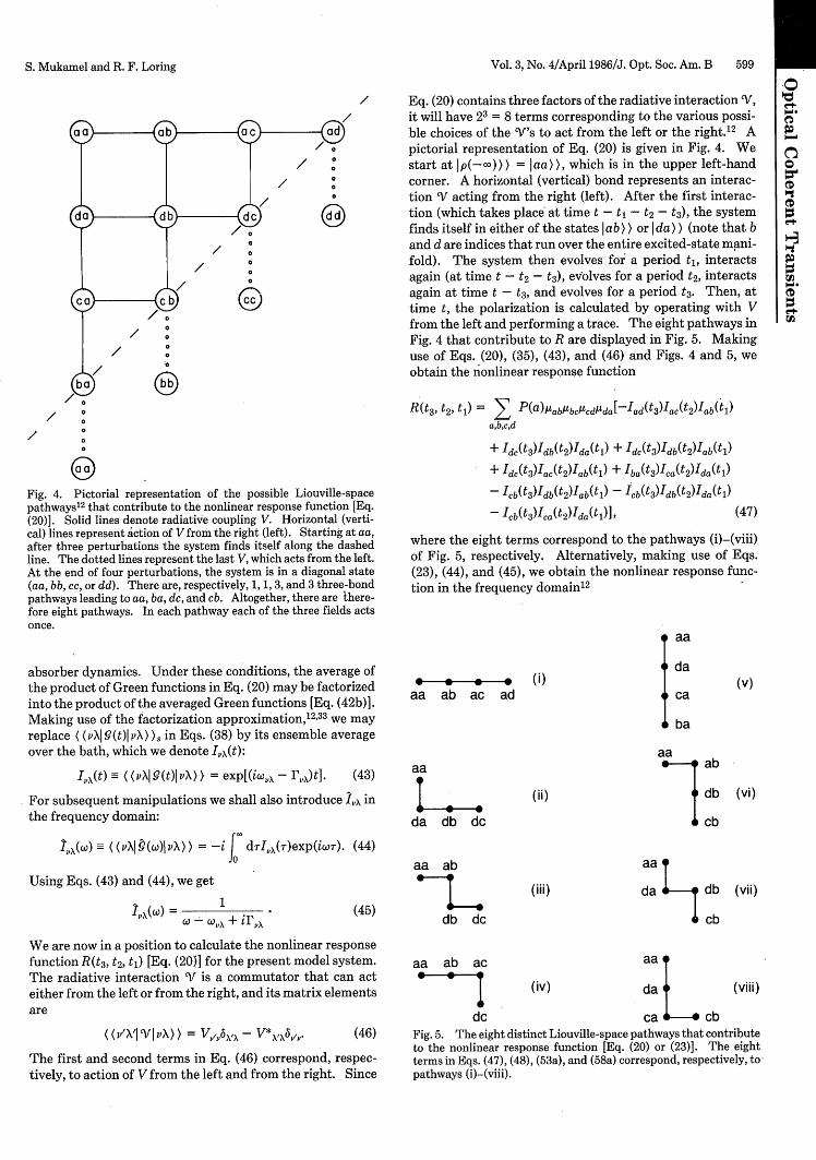
Fig. 4. Pictorial representation of the possible Liouville-spacepathways'2 that contribute to the nonlinear response function [Eq.(20)]. Solid lines denote radiative coupling V. Horizontal (verti-cal) lines represent action of V from the right (left). Starting at aa,after three perturbations the system finds itself along the dashedline. The dotted lines represent the last V, which acts from the left.At the end of four perturbations, the system is in a diagonal state(aa, bb, cc, or dd). There are, respectively, 1, 1, 3, and 3 three-bondpathways leading to aa, ba, dc, and cb. Altogether, there are there-fore eight pathways. In each pathway each of the three fields actsonce.

absorber dynamics. Under these conditions, the average ofthe product of Green functions in Eq. (20) may be factorizedinto the product of the averaged Green functions [Eq. (42b)].Making use of the factorization approximation,12 3 3 we mayreplace ( (vXj 9(t)j vX) ), in Eqs. (38) by its ensemble averageover the bath, which we denote Ix(t):

I^X(t)- ((vXI.(t)IvX)) = exp[(i~x^ - rF,)t]. (43)

For subsequent manipulations we shall also introduce Lx inthe frequency domain:

((VXl?(@)lX)) = -i f dTIx(r)exp(iw). (44)

Using Eqs. (43) and (44), we get

1 vX( ) = - O^A + (45)

We are now in a position to calculate the nonlinear responsefunction R(t3 , t2 , t1) [Eq. (20)] for the present model system.The radiative interaction V is a commutator that can acteither from the left or from the right, and its matrix elementsare

((V'X'ICVIVX)) = VV/VbA - V*X A'Av. (46)

The first and second terms in Eq. (46) correspond, respec-tively, to action of V from the left and from the right. Since

Eq. (20) contains three factors of the radiative interaction CV,it will have 23 = 8 terms corresponding to the various possi-ble choices of the V's to act from the left or the right.'2 Apictorial representation of Eq. (20) is given in Fig. 4. Westart at p(-a))) = aa)), which is in the upper left-handcorner. A horizontal (vertical) bond represents an interac-tion AY acting from the right (left). After the first interac-tion (which takes place at time t - tl- t 3 ), the systemfinds itself in either of the states l ab) ) or Ida)) (note that band d are indices that run over the entire excited-state mani-fold). The system then evolves for a period t, interactsagain (at time t - t2-t 3 ), evolves for a period t2 , interactsagain at time t - t3, and evolves for a period t3. Then, attime t, the polarization is calculated by operating with Vfrom the left and performing a trace. The eight pathways inFig. 4 that contribute to R are displayed in Fig. 5. Makinguse of Eqs. (20), (35), (43), and (46) and Figs. 4 and 5, weobtain the nonlinear response function

R(t3, t2, t,) = E P(a)IabubcpCdda[ Iad(t3)Iac(t2)Iab(tl)ab,c,d

+ Idc(t3)Idb(t2)Ida(tl) + Idc(t3)Idb(t2)Iab(tl)

+ Idc(t3)Iac(t2)Iab(tl) + Iba(t3)Ica(t2)Ida(tl)

- Icb(t3)Idb(t2)Ib(tl) - Icb(t3)Idb(t2)Ida(tl)- Icb(t3)Ica(t2)Ida(tl)]I (47)

where the eight terms correspond to the pathways (i)-(viii)of Fig. 5, respectively. Alternatively, making use of Eqs.(23), (44), and (45), we obtain the nonlinear response func-tion in the frequency domain12

_ _ _ _

aa ab ac ad

aa

da db dc

aa ab

db dc

(i)

aa

da

ca

ba

aaab

.- db

cb

(ii)

(iii)

aa

dam-t dbcb

(v)

(vi)

(vii)

aa ab ac aa

<' (iv) da (viii)

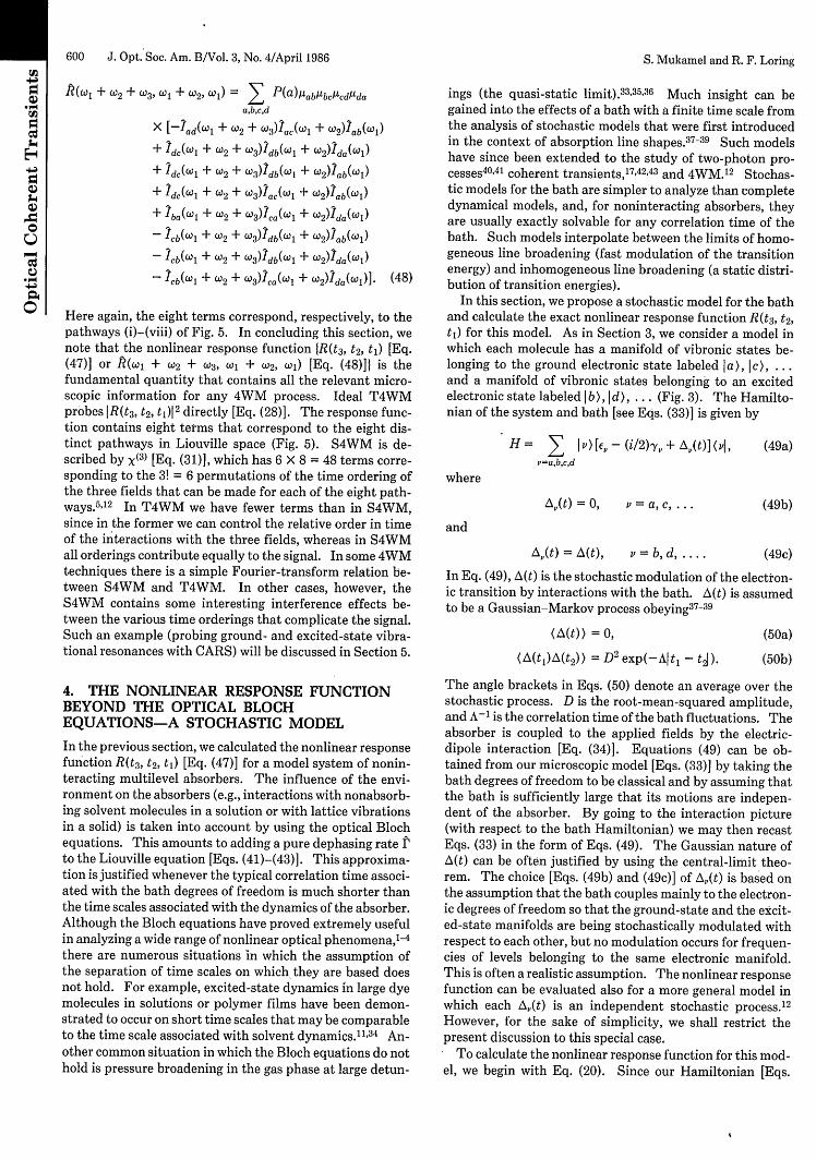
dc ca cbFig. 5. The eight distinct Liouville-space pathways that contributeto the nonlinear response function [Eq. (20) or (23)]. The eightterms in Eqs. (47), (48), (53a), and (58a) correspond, respectively, to,pathways (i)-(viii).


I .

0

a

8

)a-

To


P(W1 + @2 + WA3, W1 + W2, W) E P(a).abIbccdydaa,b,c,d

X [ ad( l + W2 + W3)Iac(Cil + W2)Iab(-l)

+ dc(W1 + W2 + W3)Idb(1 + W2)Ida(WI1)

+ dc(Wl + °2 + (3)ldb(Cl + W2)Iab(Cl)

+ 7dJ(W1 + °2 + W3)2ac("li + (C2)Iab( )

+ 7ba(cl + W2 + W3 )Ica(1W + W2)Ida(A)

- cb(- + WA2 + W3)Idb(C-l + WJ2)1ab((-1)

- cb(l + CA2 + CA3)ldb( 1 + W2)'da('l)- Icb(wl + ° 2 + A3)ca(1l + 2 )7da( CA)] (48)

Here again, the eight terms correspond, respectively, to thepathways (i)-(viii) of Fig. 5. In concluding this section, wenote that the nonlinear response function R(t3, t2, t) [Eq.(47)] or R(co + 2 + )3, cw + 2, w01) [Eq. (48)]} is thefundamental quantity that contains all the relevant micro-scopic information for any 4WM process. Ideal T4WMprobes IR(t3, t2 , t)I 2 directly [Eq. (28)]. The response func-tion contains eight terms that correspond to the eight dis-tinct pathways in Liouville space (Fig. 5). S4WM is de-scribed by x(3) [Eq. (31)], which has 6 X 8 = 48 terms corre-sponding to the 3! = 6 permutations of the time ordering ofthe three fields that can be made for each of the eight path-ways.5 "12 In T4WM we have fewer terms than in S4WM,since in the former we can control the relative order in timeof the interactions with the three fields, whereas in S4WMall orderings contribute equally to the signal. In some 4WMtechniques there is a simple Fourier-transform relation be-tween S4WM and T4WM. In other cases, however, theS4WM contains some interesting interference effects be-tween the various time orderings that complicate the signal.Such an example (probing ground- and excited-state vibra-tional resonances with CARS) will be discussed in Section 5.

ings (the quasi-static limit).33 353 6 Much insight can begained into the effects of a bath with a finite time scale fromthe analysis of stochastic models that were first introducedin the context of absorption line shapes.37-39 Such modelshave since been extended to the study of two-photon pro-cesses40' 41 coherent transients, 7 42,43 and 4WM.1 2 Stochas-tic models for the bath are simpler to analyze than completedynamical models, and, for noninteracting absorbers, theyare usually exactly solvable for any correlation time of thebath. Such models interpolate between the limits of homo-geneous line broadening (fast modulation of the transitionenergy) and inhomogeneous line broadening (a static distri-bution of transition energies).

In this section, we propose a stochastic model for the bathand calculate the exact nonlinear response function R(t3, t2,ti) for this model. As in Section 3, we consider a model inwhich each molecule has a manifold of vibronic states be-longing to the ground electronic state labeled la), c), ...and a manifold of vibronic states belonging to an excitedelectronic state labeled Ib), Id), . . . (Fig. 3). The Hamilto-nian of the system and bath [see Eqs. (33)] is given by

H = I ) [ - (i/2)y, + A,(t)] ( I ,v=a,b,c,d

where

(49a)

(49b)

and

A,(t) = A(t), v = b, d, .... (49c)

In Eq. (49), A(t) is the stochastic modulation of the electron-ic transition by interactions with the bath. A(t) is assumedto be a Gaussian-Markov process obeying3 7-39

(A(t)) = 0,

(A(tO)A(t2)) = D2 exp(-Alt, -t2l)

4. THE NONLINEAR RESPONSE FUNCTIONBEYOND THE OPTICAL BLOCHEQUATIONS-A STOCHASTIC MODEL

In the previous section, we calculated the nonlinear responsefunction R(t3, t2 , t) [Eq. (47)] for a model system of nonin-teracting multilevel absorbers. The influence of the envi-ronment on the absorbers (e.g., interactions with nonabsorb-ing solvent molecules in a solution or with lattice vibrationsin a solid) is taken into account by using the optical Blochequations. This amounts to adding a pure dephasing rate to the Liouville equation [Eqs. (41)-(43)]. This approxima-tion is justified whenever the typical correlation time associ-ated with the bath degrees of freedom is much shorter thanthe time scales associated with the dynamics of the absorber.Although the Bloch equations have proved extremely usefulin analyzing a wide range of nonlinear optical phenomena,1Athere are numerous situations in which the assumption ofthe separation of time scales on which they are based doesnot hold. For example, excited-state dynamics in large dyemolecules in solutions or polymer films have been demon-strated to occur on short time scales that may be comparableto the time scale associated with solvent dynamics."',34 An-other common situation in which the Bloch equations do nothold is pressure broadening in the gas phase at large detun-

(50a)

(50b)

The angle brackets in Eqs. (50) denote an average over thestochastic process. D is the root-mean-squared amplitude,and A- is the correlation time of the bath fluctuations. Theabsorber is coupled to the applied fields by the electric-dipole interaction [Eq. (34)]. Equations (49) can be ob-tained from our microscopic model [Eqs. (33)] by taking thebath degrees of freedom to be classical and by assuming thatthe bath is sufficiently large that its motions are indepen-dent of the absorber. By going to the interaction picture(with respect to the bath Hamiltonian) we may then recastEqs. (33) in the form of Eqs. (49). The Gaussian nature ofA(t) can be often justified by using the central-limit theo-rem. The choice [Eqs. (49b) and (49c)] of A(t) is based onthe assumption that the bath couples mainly to the electron-ic degrees of freedom so that the ground-state and the excit-ed-state manifolds are being stochastically modulated withrespect to each other, but no modulation occurs for frequen-cies of levels belonging to the same electronic manifold.This is often a realistic assumption. The nonlinear responsefunction can be evaluated also for a more general model inwhich each AO(t) is an independent stochastic process.' 2

However, for the sake of simplicity, we shall restrict thepresent discussion to this special case.

To calculate the nonlinear response function for this mod-el, we begin with Eq. (20). Since our Hamiltonian [Eqs.


A'( = , P = a, c, . . .


(49)1 is now time dependent, we need to modify Eq. (20)slightly. It should be recast in the form

R(t 3, t2 t) = ( (Vj (t1 + t2 + t3, t + t2)

X cV9(t 1 + t2 , t1 )cV9(t 1 O)CVIP(-c))), (51)

where 9(T2, rl) is the molecular evolution operator from timeT, to time 12

((VXI1(r2, 1i)vX)) = exp -i'CX(T 2 - T)

-/2 ( + YX)(r2 -T) TO i dT[A,(T) - AX(T)]} (52a)

and

( (v'X'1g(T2, r IvX) ) -= Tvvxx'( ( v ( T2, i)IvX) s (52b)

Of course, for a time-independent Hamiltonian, 9(T2, T1)reduces to 9(12 - ) [Eq. (13)], and Eq. (51) reduces to Eq.(20). The trace in Eq. (51) should now be understood toinclude an average over the stochastic process. Note thatcalculating the response function [Eq. (51)] involves averag-ing the product of three Green functions over the thermalbath. The Bloch-equation approximation involves the fac-torization of this average into the product of three averagedGreen functions [Eq. (43)].33 Our present calculation willallow us to explore the significance of this approximation.Making use of Eqs. (34) and (49)-(52), we get

R(t3, t2, t1) = E P(ajabibcycdsdaa,b,c,d

+ [-Kad(t 3 )Ka(t 2 )Kab(tl)_(t3 t2 t1 )

+ Kdc(t3)Kdb(t 2 )Kda(tl)4P (t3, t2 , t1 )

+ Kdc(t3)Kdb(t 2 )Kab(ti)4'P(t3, t2 , t1 )

+ KdC~t3)KaCt2)Kab(t1)'P+(t31 t2 t)

+ Kba(t3)Kca(t 2)Kda(tl)4 (t3, t2, t1)

- Kcb(t 3 )Kdb(t 2)Kab(tl) 4'(t3, t2 , t1 )

- KCb(t3)Kdb(t2)Kd.(t1)' D(t 3, t2, t1 )

- Kcb(t)Kca(t 2)Kda(tl)4D (t3, t2 tl)],

where

K~x(t) = exp[-icvt - /2(-Y + YX)t] '

V(t 3 t2 t) = expl-g(t 3) - g(t1 ) [g(t1 + t2 + t3)

- g(t1 + t2) - g(t2 + t3)]1,

g(t) =' d-r f dr 2 (A(rl)A(T 2))fo fo I

(53a)

(53b)

+ g(t2)(53c)

using the cumulant expansion (which is exact to secondorder for the present Gaussian-Markov model). Equation(53) should be compared with Eq. (47), which gives R(t 3 , t2,

tj) for the Bloch-equation model of Section 3. The eightterms in Eq. (53a) correspond to the eight pathways of Fig. 5,respectively. Each term in Eq. (47) is a product of a func-tion of tj, a function of t2, and a function of t3. R has thisstructure because, in the Bloch-equation approximation, theaverage of the product of three Green functions in Eq. (51)factors into the product of three averaged Green functions.For a bath of arbitrary time scale, this factorization approxi-mation no longer holds, as can be seen from Eq. (53a). Letus consider two limiting cases of Eqs. (53). In the limit offast modulation (A/D >> 1), Eq. (53c) becomes

4+(t3, t2 t) = exp[-P(t 3 + t)], (55a)

where

r = D2/A. (55b)

If this result is substituted into Eq. (53a), we recover theBloch-equation result of Section 3 [Eq. (47)]. In this limit,the line-shape function IA of Eq. (43) is related to KX(t) ofEqs. (53) by

I>x(t) = exp(-ft)KV(t). (56)

In the limit of slow modulation (A/D << 1), Eq. (53c) becomes

b(i)(t 3, t2 t) = exp[-(D 2/2)(t3 + tJ)21 (57)

Substitution of Eq. (57) into Eqs. (53) gives the nonlinearresponse function of a system with a static Gaussian distri-bution of electronic transition frequencies (inhomogeneousline broadening).

Making use of Eqs. (53) and (21), we can evaluate theresponse function in the frequency domain

R() + W2 + C03, Col + w2, 1) = P Aabybcdydaalb,c,d

[ 4 (S3 + Qad, 2 + Qac, S1 + Qab)

+ 4'(s 3 + Qdc, S2 + Qdb, S1 + Qda)

+ il +(S3 + Qdc' S2 + Qdb, Si + Qab)

+ t+(S3 + QdC, 2 Qac, S1 + Qab)

+4(S3+ ba, S2+ Qca, S1 + Qda)

- V (s3 + Qcb, S2 + Qdb, S1 + Qab)

- P+(S3 + Qcb, S2 + Qdb, S1 + Qda)

- '(S3 + QCb, 2 + Qca, S, + Oda)], (58a)

= - [exp(-At) - 1 + At]. (53d)

The functions 4'i are defined by[f+t 2+t3

4(±)(t3, t2, t1) = (exp-i drA(r) if drA(T)] ),I+t 2

(54)

where the angle brackets denote averaging over the stochas-tic process A(r). The average in Eq. (54) was evaluated by

where

S, = -icol,

S2 = -i(Col + cc2),

S3 = -i(Cl + cc2 + C3),

QA= ivx + (1/ 2 )("Y + yx).

The functions AA are defined as follows:

(58b)

(58c)

(58d)

(58e)

S. Mukamel, and R. F. Loring


/'4(S 3, S2, S) =fj dt 3 f dt 2 fo dt,

X exp[-sltl - s2t2 - s3t 3]/A:(t3, t2 t). (59)

In Appendix A, we outline a convenient computationalmethod for evaluating this triple integral using a simplerecursive formula.40 '4 ' Note that x(3) may be obtained bysimply permuting the frequency factors in R. according toEq. (31).

There is currently great interest in the application of4WM to obtain dynamical information from systems whoseabsorption line shape is dominated by static inhomogeneousbroadening10"11,14-17,2834,44 The information content of4WM observables is usually established on the basis of theBloch equations. The more general model of this sectioncan be used to gain further insight into the line-narrowingcapabilities of time- and frequency-resolved 4WM experi-ments. The information content of specific nonlinear spec-troscopic observables for a system interacting with a bath ofarbitrary time scale can be analyzed using the present mod-el.

5. COHERENT RAMANSPECTROSCOPY-GROUND-STATE VERSUSEXCITED-STATE CARS

As an example of the way in which the present work can beused to establish the relationships between T4WM andS4WM, we consider coherent Raman measurements[CARS and coherent Stokes Raman spectroscopy(CSRS)].1026-32 45 46 These experiments usually involve twofields (i.e., k3 = k), and the signal mode is

k = 2k -k 2 , (60a)

Ws = 2w1 -c 2. (60b)

We shall start with an ideal S4WM and focus on x(3) [Eq.(31)]. Since two fields are equal, there are only three per-mutations of the frequencies (and not six). Setting 2 equalto - 2 in Eq. (31) and writing the frequency permutationsexplicitly, we get

X(3)(_(," .1' - 2, WO) = (2w, - 2, 1 - 02, WO)

+ (2w - 2, 1-2, -'02)

+ (2,ol - 2, 2w1 , co,), (61)

where R is given in Eq. (48). X3

) thus contains 3 X 8 = 24terms. In CARS we look for two-photon resonances in thesignal that occur when w - 2 equals an energy differencebetween two ground-state or excited-state vibrationalstates. For our level scheme (Fig. 3) such resonances occurfor - 2 = +Wca or for w - 2 = +wdb. The labels CARSand CSRS refer to the cases in which w > 2 and w < 2 ,

respectively. Since there are no fundamental differencesbetween the theoretical treatments of the two, we shall focuson the CARS resonances

1 W2 = oca (62a)

and

(AI- 02 = Odb-

Equation (62a) represents ground-state CARS, and Eq.(62b) represents excited-state CARS. For the sake of clar-ity and simplicity, we shall restrict the present analysis tcthe optical Bloch equations (Section 3). The generalizationto the stochastic model is straightforward and can be madeby replacing each of the relevant terms in Eq. (48) by itscounterpart in Eqs. (58). From Eq. (48) it is clear thatCARS resonances [Eqs. (62)] can come only from the middleGreen function. We shall thus consider only the terms con-tainingIa(c ol - c 2) and Idb(w1 -CO2). It is also clear from Eq.(61) that the third term R(2col - 2, 2col, co,) cannot contrib-ute to CARS, since its two-photon resonances are at 2col andnot at w, - 02. We shall therefore ignore this term. Let usdenote the eight diagrams of the first term in Eq. (61) by(i)-(viii) and the corresponding ones for the second term inEq. (61) by (i)' . . . (viii)' (see Fig. 5). Starting with ground-state CARS, we note that there are four terms containingIca(W - 02). These correspond to diagrams (v), (viii), (v)',and (viii)', i.e.,

Xca = E P(a) b bc-cdYda ba(2cj w 2)ca(w1 - 02)b,d

- Zcb(2l - W2)lca(W1 - Co2)]

X [2dca(w) + 7da( °W2)], (63)

where the subscript in ca denotes that these are ground-state ( - 2 = ca) resonances. We shall now invoke therotating-wave approximation (RWA) in which we retainonly resonant terms, in which all denominators contain adifference of a field frequency and a molecular optical fre-quency, and neglect all terms in which at least one denomi-nator is antiresonant. For the ground-state CARS, the onlyterm that survives is diagram (v):

Xca = E P(a)ab-bc cdwdak(2- 2)Ica(-l - -2)da(l).b,d

(64)

Similarly, for the excited-state CARS we have eight terms inEq. (61) that contain db(Wl - 2 ). These correspond topathways (ii), (iii), (vi), and (vii) and (ii)', (iii)', (vi)', and(vii)':

Xdb 3 = ZP(a)abIbccdda[7dc(2-1 - -2)7db(co1 - W2)a,c

- 1cb(2w1 - '2)7db(01 - 2)]

X [7da("') + 7da( C02) + ab(Wl) + 7ab& °2)]. (65)

Within the RWA, only two terms contribute to Xdb(, whichcome from pathways (ii) and (iii)', i.e.,

Xdb = Z P(a)abIbcccdcdaac

X dc(2w - 2)7db(w-l cW2)[Zda(w, + ab(£02)]- (66)

Making use of the explicit form of 7,x(w) [Eq. (45)] and Eqs.(62b) (64) and (66), we therefore have

S. Mukarnel and R. F. Loring


Xca = P(a)8ta bbcycdyda 2w, - W2 - Wba + rbab,d

X1 1

W1 2 )ca + irca 1 - da + irda(67a)

and

Xdb (3 = E P(a)abbcycddaa,c

X1 1

2 -2 - Wdc + L]dc @1 W CA2 - Wdb + idb

[@ - da + iTda + - 2 +-lab + irab]Equations (67) show that the excited-state CARS arisesfrom two pathways that interfere, whereas the ground-stateCARS is associated with only one pathway. To make theinterference in Eq. (67b) more explicit, we rearrange it in theform

Xdb = P(a)abibcpcdydaa,c

X1 1

2 w1c-2 W2(dc +irdc Wl Wda +irda

shape, E(t), and that the pulse duration is short comparedwith T. Since the last interaction has to be with co,, there areonly two permutations of frequencies that will contribute toEq. (19):

P(k,, t) = (-i)' J dt3 J dt 2 J dt, R(t, t2 t)

X E(t - t3- T)exp[i(2 , - -2)t3E*(t -t2-t3)

X E(t - tl - t2 - t)exp[iolt, + i(w1 -2)t2]

+ E(t - t2- t3)E*(t -tl - t2- t3)

X exp[-i2tl + i(,l- 2)t2l-(70)

Equation (70) is the time-domain analog of Eq. (61) andcontains 16 terms. We now make the following assump-tions: The pulse envelope E(r) is sufficiently long that itsspectral bandwidth is narrow enough to select a particularresonance (co - 2 = db or -c - = Wac) We furtherassume the RWA so that the same terms that contribute inthe frequency domain will contribute here. On the otherhand, we take the pulses to be sufficiently short that I(t)cannot evolve appreciably during the pulses. We can there-fore select the same terms that contributed to Eqs. (63) and(65) and set

E(r) = E(r)

in Eq. (70). We then get for the ground-state CARS

(71)

x 1 ' b[+-C02 - ab + irab °1- 2 Wdb + irdbI

(68)

where

r ab+ rad- rbd = a + ab + ad - bd- (69)The CARS resonance is contained in the term in Eq. (68)that is proportional to . When la) is the actual groundvibronic state, Ya = 0, and P is then a combination of pure-dephasing widths that vanishes in the absence of pure de-phasing. The two pathways thus interfere destructively,and, in the absence of pure dephasing, the CARS excited-state resonance disappears. In the presence of pure dephas-ing, the cancellation is not complete, and a dephasing-in-duced resonance appears. Such resonances have been ob-served experimentally. They have been denoted PIER4(pressure-induced extra resonance in four-wave mixing) 9

and DICE (dephasing-induced coherent emission).10Equations (67) and (68) show that in S4WM there is a

fundamental difference between the ground-state and theexcited-state CARS resonances. The interference in Eq.(66) occurs between two pathways in which the first interac-tion occurs, respectively, with w1 and with -C2 In a S4WMwe have no control over the relative order in time of bothinteractions. Both pathways contribute equally, and theyinterfere. The situation is quite different when the CARSexperiment is done in the time domain (T4WM). A time-domain CARS experiment is usually performed by sendingtwo time-coincident pulses with wave vectors k, and k2 intothe sample. After a variable delay, T, a second k, pulse isapplied, and the total coherent emission at k, = 2k, - k2 isdetected. We shall assume that all pulses have the same

Pca(ks, t) = E P(a)abAbcucdhdaba(t - T)Ica(T)a,bc,d

(72a)X exp[i(2, - 2t- icaT]

and for the excited-state CARS

Pdb(kS, t) = 2E' ac P(a)AabbccdudaId(t - T)Idb(T)alb,c,d

X exp[i(2col - w2 )t - iT]. (72b)

The frequency-domain interference of Eq. (67b) is no longerpresent. The system does not have time to evolve betweenthe first two interactions, and the two pathways that con-tribute to Eq. (72b) [(ii) and (iii)'] give an identical contribu-tion. When the signal is probed as a function of T at t = T,we have

Sca(T) I Ia(T)I' = exp(-2rcaT) (73a)

and

Sdb(T) Idb(T)I| = exp(-2rdbT). (73b)

The time domain CARS can be used to probe excited-stateresonances even in the absence of pure dephasing, since thedestructive interference of the frequency-domain CARS dis-appears. This point was discussed recently by Weitekampet al.32 The present analysis clarifies the origin of thisdifference.

6. CONCLUDING REMARKS

In this paper we developed a general theory of 4WM process-es in terms of the nonlinear response function of the nonlin-



ear medium R(t 3 , t2, t). The response function is an intrin-sic molecular property that contains all the microscopic in-formation relevant to any type of 4WM process. The detailsof a particular 4WM experiment are contained in the exter-nal fields, El(t), E2 (t), E3 (t), and in the particular choice ofthe observable mode k,. The generated signal is calculatedby convolving the response function with the external fieldsand choosing k, [Eq. (19) or (22)]. Itisonlyatthisstagethatthe distinction is made among the various 4WM techniques(photon echo, transient grating, CARS, CSRS, etc.). Wehave shown that the response function contains eight terms(Fig. 5). We can express each term using the four-pointcorrelation function of the dipole operator, i.e.,

F(-rl, T2, T3, 4) Tr[V(-r1)V(T2)V(7 3) V(7 4)p(-o)]

= (V('r1)V(2)V(r 3)V(,)4), (74a)

where

V(r) = exp(iHr) V exp(-iHr).

radiative interactions. In a steady-state experiment(S4WM), however, all time orderings contribute equally.The T4WM is therefore simpler, and some interesting inter-ference effects may show up in S4WM. This was demon-strated in our discussion of ground-state and excited-stateCARS in Section 5.

APPENDIX A

We wish to evaluate VA [Eq. (59)], which is the triple Laplacetransform of d>+ [Eq. (53c)]. Following Takagahara et al.4 0

and Mukamel,4' we shall first write Eq. (53c) explicitly,using Eq. (53d), as

(Tr1, r 2, 3) = expj-g(-r) - g(r3)

+ n exp(-Ai- 2 )[1 - exp(-Ai-l)][1 - exp(-AT3 )]}, (Al)

where

(74b) = D2/A2 .

Here, H is the molecular Hamiltonian [Eqs. (33)], and V isthe dipole operator [Eq. (34)]. In terms of this four-pointcorrelation function, we have'2

R(t3, t2 t) = -F(O, t, t1 + t2 t + t2 + t3)

+ F(tj, t + t2 t + t2 + t3 0)

+ F(O, t + t 2 tl + t2 + t3 t)

+ F(O, t, t + t2 + t3 , tl + t2)

+ F(t, + t2 + t3 t + t2, t1l, 0)

- F(O, t1 + t2 + t3, t + t2 t)

- F(tj, t + t2 + t3 t + t2, 0)

-F(t, + t2 t + t2 + t3 t, 0), (75)

where the eight terms correspond, respectively, to diagrams(i)-(viii) of Fig. 5. It is therefore clear that the various 4WMprocesses probe different features of the four-point correla-tion function of the dipole operator. The response functiondiscussed in this article is closely related to that introducedby Butcher. 2 Our time arguments t, t2 , and t3 (Fig. 2) werechosen, however, differently. With the present choice, therelations between T4WM and S4WM are clearer. Since theresponse function is probing the four-point correlation func-tion [Eqs. (74) and (75)], it necessarily contains more infor-mation than the ordinary absorption line shape that is givenby the two-time correlation function ( V(-) V(O)). This canbe utilized, e.g., to eliminate inhomogeneous broadening se-lectively, as is done in photon echoes.' 4-17 The extra reso-nances (PIER4, DICE)9 10 discussed in Section 5 can be alsoused selectively to eliminate inhomogeneous broadening.We have evaluated R for a stochastic model for a bath withan arbitrary time scale. Our solution [Eqs. (53) or (58)] is ageneralization of the results of the optical Bloch equationsand reduces to that solution in the limit of fast modulation.The stochastic expression for R permits a better under-standing of the interplay between homogeneous and inho-mogeneous broadening in 4WM. We further note that inT4WM we may control the order in time of the various

(A2)

If we expand Eq. (Al) in a Taylor series in exp(-AT2) andsubstitute back into Eq. (59), we can carry out the T2 integra-tion resulting in

0' (S1, S2, s3) = 8 + Jn(S)jn(S3)n=0

(A3)

where

Jn(S) = J dT[l - exp(-Ar)]n exp[-sr - g(-)]. (A4)fo

On integrating Eq. (A4) by parts, we get the recursion rela-tions

7AJn+(s) = nAJn-,(s) - (s + nA)Jn(s), n = 1, 2,(A5)

and

7AJi(s) = - sJ0 (s). (A6)

Equations (A5) and (A6) can now be used to generate acontinued fraction representation of Jo

Jo(s) =

+s + A +

1

2D2

s + 2A+ 3D2

s + 3A + .... (A7)

Equations (A5)-(A7) allow us to calculate Jn recursively.

ACKNOWLEDGMENTS

The support of the National Science Foundation, the U.S.Office of Naval Research, the U.S. Army Research Office,and the donors of the Petroleum Research Fund adminis-tered by the American Chemical Society is gratefully ac-knowledged. We thank D. Wiersma for useful discussions.Special thanks go to June M. Rouse for the careful typing.

Shaul Mukamel is a Camille and Henry Dreyfus tea-cher-scholar.



REFERENCES

1. N. Bloembergen, Nonlinear Optics (Benjamin, New York,1965).

2. P. N. Butcher, Nonlinear Optical Phenomena (Ohio U. Press,Athens, Ohio, 1965).

3. M. D. Levenson, Introduction to Nonlinear Laser Spectrosco-py (Academic, New York, 1982).

4. Y. R. Shen, The Principles of Nonlinear Optics (Wiley, NewYork, 1984).

5. N. Bloembergen, H. Lotem, and R. T. Lynch, "Lineshapes incoherent resonant Raman scattering," Indian J. Pure Appl.Phys. 16, 151 (1978).

6. S. A. J. Druet and J. P. E. Taran, "CARS spectroscopy," Prog.Quantum Electron. 7, 1 (1981).

7. T. K. Lee and T. K. Gustafson, "Diagrammatic analysis of thedensity operator for nonlinear optical calculations: pulsed andcw responses," Phys. Rev. A 18, 1597 (1978).

8. J. L. Oudar and Y. R. Shen, "Nonlinear spectroscopy by multi-resonant four-wave mixing," Phys. Rev. A 22, 1141 (1980).

9. Y. Prior, A. R. Bogdan, M. Dagenais, and N. Bloembergen,"Pressure-induced extra resonances in four-wave mixing,"Phys. Rev. Lett. 46, 111 (1981); A. R. Bogdan, M. W. Downer,and N. Bloembergen, "Quantitative characteristics of pressure-induced four-wave mixing signals observed with cw laserbeams," Phys. Rev. A 24, 623 (1981); L. J. Rothberg and N.Bloembergen, "High resolution four-wave light mixing studiesof collision-induced coherence in Na vapor," Phys. Rev. A 30,820 (1984).

10. J. R. Andrews and R. M. Hochstrasser, "Thermally inducedexcited-state -coherent Raman spectra of solids," Chem. Phys.Lett. 82, 381 (1981); J. R. Andrews, R. M. Hochstrasser, and H.P. Trommsdorff, "Vibrational transitions in excited states ofmolecules using coherent Stokes Raman spectroscopy: appli-cation to ferrocytochrome-C," Chem. Phys. 62, 87 (1981).

11. T. Yajima and H. Souma, "Study of ultra-fast relaxation pro-cesses by resonant Rayleigh-type optical mixing. I. Theory,"Phys. Rev. A 17,309 (1978); T. Yajima, H. Souma, and Y. Ishida,"Study of ultra-fast relaxation processes by resonant Rayleigh-type optical mixing. II. Experiment on dye solutions," Phys.Rev. A 17, 324 (1978).

12. S. Mukamel, "Non-impact unified theory of four-wave mixingand two-photon processes," Phys. Rev A 28, 3480 (1983).

13. V. Mizrahi, Y. Prior, and S. Mukamel, "Single atom versuscoherent pressure induced extra resonances in four-photonprocesses," Opt. Lett. 8, 145 (1983); R. W. Boyd and S. Muka-mel, "The origin of spectral holes in pump-probe studies ofhomogeneously broadened lines," Phys. Rev. A 29, 1973 (1984).

14. I. D. Abella, N. A. Kurnit, and S. R. Hartmann, "Photonechoes," Phys. Rev. 141, 391 (1966); S. R. Hartmann, "Photon,spin, and Raman echoes," IEEE J. Quantum Electron. 4, 802(1968); T. W. Mossberg, R. Kachru, A. M. Flusberg, and S. R.Hartmann, "Echoes in gaseous media: a generalized theory ofrephasing phenomena," Phys. Rev. A 20, 1976 (1979).

15. W. H. Hesselink and D. A. Wiersma, "Theory and experimentalaspects of photon echoes in molecular solids," in Modern Prob-lems in Condensed Matter Sciences, V. M. Agranovich and A.A. Maradudin, eds. (North-Holland, Amsterdam, 1983), Vol. 4,p. 249.

16. R. W. Olson, F. G. Patterson, H. W. H. Lee, and M. D. Fayer,"Delocalized electronic excitations of pentacene dimers in a p-terphenyl host: picosecond photon echo experiments," Chem.Phys. Lett. 78, 403 (1981).

17. R. F. Loring and S. Mukamel, "Unified theory of photon echoes:the passage from inhomogeneous to homogeneous line broaden-ing," Chem. Phys. Lett. 114, 426 (1985).

18. J. R. Salcedo, A. E. Siegman, D. D. Dlott, and M. D. Fayer,"Dynamics of energy transport in molecular crystals: the pico-second transient grating method," Phys. Rev. Lett. 41, 131(1978).

19. M. D. Fayer, "Dynamics of molecules in condensed phases:picosecond holographic grating experiments," Ann. Rev. Phys.Chem. 33, 63 (1982).

20. P. F. Liao, L. M. Humphrey, and D. M. Bloom, "Determination

of upper limits for spatial energy diffusion in ruby," Phys. Rev.B 10, 4145 (1979).

21. J. K. Tyminski, R. C. Powell, and W. K. Zwicker, "Investigationof four-wave mixing in NdxLa1-xP5O 4 ,` Phys. Rev. B 29, 6074(1984).

22. H. J. Eichler, "Laser-induced grating phenomena," Opt. Acta24, 631 (1977).

23. A. von Jena and H. E. Lessing, "Theory of laser-induced ampli-tude and phase gratings including photoselection, orientationalrelaxation, and population kinetics," Opt. Quantum Electron.11, 419 (1979).

24. R. F. Loring and S. Mukamel, "Microscopic theory of the tran-sient grating experiment," J. Chem. Phys. 83, 4353 (1985); "Ex-tra resonance in four-wave mixing as a probe of exciton dynam-ics: the steady-state analog of the transient grating," J. Chem.Phys. 84, 1228 (1986).

25. N. Bloembergen, "The stimulated Raman effect," Am. J. Phys,35, 989 (1967).

26. A. Laubereau and W. Kaiser, "Vibrational dynamics of liquidsand solids investigated by picosecond light pulses," Rev. Mod.Phys. 50,607 (1978); W. Zinth, H.-J. Polland, A. Laubereau, andW. Kaiser, "New results on ultrafast coherent excitation ofmolecular vibrations in liquids," Appl. Phys. B 26, 77 (1981).

27. S. M. George, A. L. Harris, M. Berg, and C. B. Harris, "Picosec-ond studies of the temperature dependence of homogeneousand inhomogeneous linewidth broadening in liquid aceto-nitrile," J. Chem. Phys. 80, 83 (1984).

28. R. F. Loring and S. Mukamel, "Selectivity in coherent transientRaman measurements of vibrational dephasing in liquids," J.Chem. Phys. 83, 2116 (1985).

29. I. I. Abram, R. M. Hochstrasser, J. E. Kohl, M. G. Semack, andD. White, "Coherence loss for vibrational and librational excita-tions in solid nitrogen," J. Chem. Phys. 71,153 (1979); F. Ho, W.S. Tsay, J. Trout, S. Velsko, and R. M. Hochstrasser, "Picosec-ond time-resolved CARS in isotopically mixed crystals of ben-zene," Chem. Phys. Lett. 97,141 (1983); S. Velsko, J. Trout, andR. M. Hochstrasser, "Quantum beating of vibrational factorgroup components in molecular solids," J. Chem. Phys. 79, 2114(1983).

30. E. L. Chronister and D. D. Dlott, "Vibrational energy transferand localization in disordered solids by picosecond CARS spec-troscopy," J. Chem. Phys. 79, 5286 (1984); C. L. Schosser and D.D. Dlott, "A picosecond CARS study of vibron dynamics inmolecular crystals: temperature dependence of homogeneousand inhomogeneous linewidths," J. Chem. Phys. 80, 1394(1984).

31, B. H. Hesp and D. A. Wiersma, "Vibrational relaxation in neatcrystals of naphthalene by picosecond CARS," Chem. Phys.Lett. 75, 423 (1980).

32. D. P. Weitekamp, K. Duppen, and D. A. Wiersma, "Delayedfour-wave mixing spectroscopy in molecular crystals: a non-perturbative approach," Phys. Rev. A 27, 3089 (1983).

33. S. Mukamel, "Collisional broadening of spectral line shapes intwo-photon and multiphoton processes," Phys. Rep. 93, 1(1982).

34. A. M. Weiner, S. DeSilvestri, and E. P. Ippen, "Three-pulsescattering for femtosecond dephasing studies: theory and ex-periment," J. Opt. Soc. Am. B 2, 654 (1985).

35. R. G. Breene, Theories of Spectral Line Shape (Wiley, NewYork, 1981).

36. K. Burnett, "Collisional redistribution of radiation," Phys. Rep.118, 339 (1985).

37. N. Bloembergen, E. M. Purcell, and R. V. Pound, "Relaxationeffects in nuclear magnetic resonance absorption," Phys. Rev.73, 679 (1948).

38. P. W. Anderson and P. R. Weiss, "Exchange narrowing in para-magnetic resonance," Rev. Mod. Phys. 25, 269 (1953).

39. R. Kubo, "A stochastic theory of line-shape and relaxation," inFluctuations, Relaxation and Resonance in Magnetic Sys-tems," D. ter Haar, ed. (Plenum, New York, 1962), p. 23.

40. T. Takagahara, E. Hanamura, and R. Kubo, "Stochastic modelsof intermediate state interaction in second order optical pro-cesses-stationary response. I," J. Phys. Soc. Jpn. 43, 802(1977); "Stochastic models of intermediate state interaction in



second order optical processes-stationary response. II," J.Phys. Soc. Jpn. 43, 811 (1977); "Stochastic models of intermedi-ate state interaction in second order optical processes-tran-sient response," J. Phys. Soc. Jpn. 43, 1522 (1977).

41. S. Mukamel, "Stochastic theory of resonance Raman lineshapes of polyatomic molecules in condensed phases," J. Chem.Phys. 82, 5398 (1985).

42. E. Hanamura, "Stochastic theory of coherent optical tran-sients," J. Phys. Soc. Jpn. 52, 2258 (1983); "Stochastic theory ofcoherent optical transients. II. Free induction decay in Pr+3:LaF 3 ," J. Phys. Soc. Jpn. 52, 3678 (1983); H. Tsunetsugu, T.Taniguchi, and E. Hanamura, "Exact solution for two levelelectronic system with frequency modulation under laser irra-diation," Solid State Commun. 52, 663 (1984).

43. M. Aihara, "Non-Markovian theory of nonlinear optical phe-nomena associated with the extremely fast relaxation in con-densed matter," Phys. Rev. B 25, 53 (1982).

44. G. J. Small, "Persistent nonphotochemical hole burning and thedephasing of impurity electronic transitions in organic glasses,"in Spectroscopy and Excitation Dynamics of Condensed Mo-lecular Systems, V. M. Agranovich and R. M. Hochstrasser, eds.(North-Holland, New York, 1983), pp. 515; T. C. Caau, C. K.Johnson, and G. J. Small, "Multiresonant four-wave mixingspectroscopy of pentacene in naphthalene," J. Phys. Chem. 89,2984 (1985).

45. B. S. Hudson, W. H. Hetherington, S. P. Cramer, I. Chabay, andG. K. Klauminzer, "Resonance enhanced coherent anti-StokesRaman scattering," Proc. Natl. Acad. Sci. (USA) 73, 3798(1976).

46. L. A. Carreira, T. C. Maguire, and T. B. Malloy, "Excitationprofiles of the coherent anti-Stokes resonance Raman spectrumof d-carotene," J. Chem. Phys. 66, 2621 (1977).

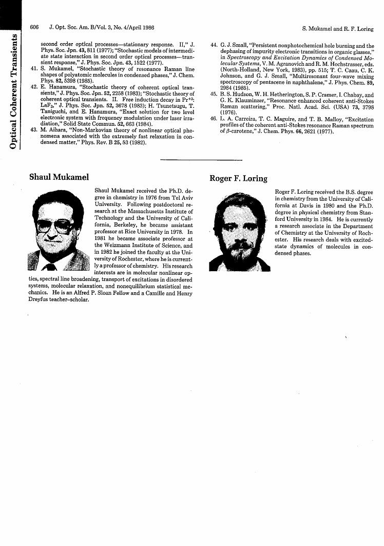
Roger F. LoringShaul Mukamel received the Ph.D. de-gree in chemistry in 1976 from Tel AvivUniversity. Following postdoctoral re-search at the Massachusetts Institute ofTechnology and the University of Cali-fornia, Berkeley, he became assistant

E, 7professor at Rice University in 1978. In1981 he became associate professor atthe Weizmann Institute of Science, andin 1982 he joined the faculty at the Uni-

g, _ versity of Rochester, where he is current-Z ly a professor of chemistry. His research

interests are in molecular nonlinear op-tics, spectral line broadening, transport of excitations in disorderedsystems, molecular relaxation, and nonequilibrium statistical me-chanics. He is an Alfred P. Sloan Fellow and a Camille and HenryDreyfus teacher-scholar.

Roger F. Loring received the B.S. degreein chemistry from the University of Cali-fornia at Davis in 1980 and the Ph.D.degree in physical chemistry from Stan-ford University in 1984. He is currentlya research associate in the Departmentof Chemistry at the University of Roch-ester. His research deals with excited-state dynamics of molecules in con-densed phases.

Shaul Mukamel


Documents

Nonlinear response function for time-domain and frequency-domain four-wave mixing