Nonlinear Receding Horizon Control of Thickness and

87 © 2012 ISIJ

ISIJ International, Vol. 52 (2012), No. 1, pp. 87–95

Nonlinear Receding Horizon Control of Thickness and Tension in a Tandem Cold Mill with a Variable Rolling Speed

Kohei OZAKI,1) Toshiyuki OHTSUKA,2) Kenji FUJIMOTO,3) Akira KITAMURA4) and Makishi NAKAYAMA5)

1) Mitsubishi Heavy Industries, Ltd., 1-1 Shinhama, 2-chome, Arai-cho, Takasago City, Hyogo, 676-8686 Japan.2) Graduate School of Engineering Science, Osaka University, 1-3 Machikaneyama, Toyonaka, Osaka, 560-8531 Japan.3) Graduate School of Engineering, Nagoya University, Furo-cho, Chikusa-ku, Nagoya-shi, Aichi, 464-8603 Japan.4) Graduate School of Engineering, Tottori University, 4-101 Koyama-Minami, Tottori, 680-8552 Japan.5) Kobe Steel, Ltd., 1-5-5 Takatsukadai, Nishi-ku, Kobe, Hyogo, 651-2271 Japan.

(Received on May 25, 2011; accepted on August 29, 2011; originally published in Tetsu-to-Hagané,Vol. 96, 2010, No. 7, pp. 459–467)

For the precise control of tension and thickness in a tandem cold mill during acceleration and deceler-ation, we have developed a nonlinear model including the rolling speed as a time-varying parameter. It isdemonstrated from simulation results that nonlinear receding horizon control by real-time optimizationresults in a satisfactory performance for the nonlinear model.

KEY WORDS: receding horizon control; tandem cold mill; nonlinear model; real-time optimization.

1. Introduction

In recent years, quality improvement through the produc-tion of high-tension steel sheets and further improvement ofthe yield have been required for the cold-rolling process.Therefore, in a tandem cold mill, highly precise control ofthe thickness at the exit of each stand and the tensionbetween the stands is necessary including precise controlduring acceleration and deceleration.

Conventionally, in steady-state high-speed rolling, thetandem cold mill is controlled using an approximate linearmodel of rolling.1,2) However, when the rolling speed changesrapidly, such as during periods of acceleration and deceler-ation, the effect of nonlinear dynamics, which has an unde-sirable influence on thickness and tension control, is notnegligible, and the linearized model is often inaccurate,resulting in variations in quality. Although a method ofdetermining gains based on a transfer function modeldepending on the rolling speed has been proposed,3) thetransfer function used was essentially a linear model underthe assumption of a constant rolling speed, and a rapidchange in the rolling speed inevitably deteriorated the con-trol performance. Hence, in this paper, a rolling model isdeveloped to express the dependence of the nonlineardynamics on the rolling speed. Moreover, a control methodis proposed for precise control of the thickness and tensioneven during acceleration and deceleration.

Although it is generally difficult to analytically design acontrol system for a nonlinear system, receding horizon con-trol (RHC)4) has drawn considerable attention as a controlmethod that is applicable to a wide variety of problems. RHCis also known as model predictive control (MPC). In RHC, thecontrol response is optimized over a finite future at eachsampling time, which results in state feedback and a high com-

putational load for nonlinear systems. A real-time algorithm,C/GMRES,5,6) has been developed as a fast computation meth-od of nonlinear RHC (NRHC) for mechanical systems with asampling period of millisecond order and has been successfullyimplemented in some applications.7–9) In this paper, NRHC isapplied to control the thickness and tension in a tandem coldmill with the rolling subjected to acceleration and decelera-tion. The control performance and computational time ofNRHC are evaluated in numerical simulations.

2. C/GMRES Algorithm for NRHC

2.1. RHC ProblemEvery function is assumed to be differentiable as many

times as necessary hereafter. Let be the state vec-tor, let be the input vector of a general nonlinearsystem, and let be the vector of time-varyingparameters given as functions of time. The state equation ofa controlled system is given by

......................... (1)

where denotes an -dimensional vector-valued function.Moreover, constraints on the state and input are expressedas the following equality constraint:

......................... (2)

where denotes an -dimensional vector-valued func-tion. An inequality constraint can be converted into anequality constraint by introducing a dummy variable.7) InRHC, an optimal control problem is solved at each time to minimize the following performance index:

... (3)

x t n( )∈u t mu( )∈

p tmp( )∈

x f x t u t p t= ( ( ), ( ), ( )),

f n

C x t u t p t( ( ), ( ), ( )) ,= 0

C mc

t

J x t T p t T L x t u t p t tt

t T= + + + ′ ′ ′ ′

+

∫φ( ( ), ( )) ( ( ), ( ), ( )) ,d

© 2012 ISIJ 88

ISIJ International, Vol. 52 (2012), No. 1

where φ and L are scalar-valued functions, and the perfor-mance index is defined so that its minimization results in thedesired control performance. The horizon of the perfor-mance index is given by [t, t + T], an interval from the cur-rent time t to T seconds later, which is a feature of RHC.That is, the initial state for the optimal control problem isgiven by the state x(t) at the current time t. The optimal con-trol input u*(t′; x(t), T) minimizing J is determined for t′ [t,t + T ], and only its initial value u*(t; x(t), T), correspondingto the current time t, is used as the actual control input u(t)to the system. Since the optimal control u* depends on thestate x(t) at each time t, RHC defines a state feedback con-trol law given by the following equation.

....................... (4)

2.2. Necessary Conditions for OptimalityLet τ = t′ − t be a fictitious time on the horizon. The prob-

lem to be solved at each time t in RHC is an optimal controlproblem over the fictitious time τ with the initial state at τ =0 given by x(t). The necessary conditions for optimality inthis problem are obtained by the calculus of variations.10)

Then, the necessary conditions for optimality are discretizedfor numerical solution by dividing the horizon [t, t + T ] intoN steps. The discretization step of the horizon is denoted byΔτ := T/N, and the state vector, the costate vector (adjointvariables), the time-varying parameter, the control input,and the Lagrange multiplier at the ith step on the discretizedhorizon are denoted by , , (i = 0, . . . , N), , and (i = 0, . . . , N −1), respectively. The costate corresponds to the Lagrangemultiplier for the state equation regarded as a constraint.Then, the discretized necessary conditions for optimality aregiven by the following equations:

........... (5)

................................. (6)

............ (7)

....................... (8)

........ (9)

.................... (10)

where H denotes the Hamiltonian defined as

........ (11)

and suffixes x and u represent partial derivatives.Equations (5)–(10) define a two-point boundary-value

problem (TPBVP) for unknowns , , , and. At each time t, the TPBVP is solved for the measured

state = x(t). Note that the TPBVP depends on time tand is not discretized with respect to t at this stage of prob-lem formulation.

2.3. C/GMRES AlgorithmA vector consisting of the control input

and the Lagrange multiplier is defined as

....... (12)

where m := mu + mc. Note that and are deter-mined as functions of U(t) and x(t) by Eqs. (5), (6), (9), and(10). That is, for a given U(t) and x(t), is determinedby Eqs. (6) and (5), and is determined by Eqs. (10)and (9). Therefore, U(t) is the unknown quantity to be deter-mined by solving the following mN-dimensional equation,which consists of Eqs. (7) and (8).

...... (13)

If U(t) is determined by solving this equation, the actual con-trol input u(t) is obtained by the projection P0:

...................... (14)

An iterative method such as the Newton method is inef-ficient and requires a long computational time to obtain U(t)by solving the mN-dimensional nonlinear equation given byEq. (13). Hence, we consider updating U(t) so as to stabilizeF = 0 instead of solving F = 0 by an iterative method at eachtime. That is, the solution at the initial time, U(0), is deter-mined so that

........................ (15)

is satisfied, and U(t) is updated so that

............ (16)

is satisfied, where denotes a damping factor used tostabilize F = 0. An equation for is obtained from Eq.(16) as follows.

...................... (17)

By solving this linear equation for and integrating in real time, U(t) can be updated without using an iterativemethod. In particular, the linear equation for can besolved efficiently by one of the Krylov subspace methodssuch as GMRES (Generalized Minimum RESidual meth-od).11) The overall algorithm is called C/GMRES6) becauseit combines the continuation method and GMRES.

3. Nonlinear Model of a Tandem Cold Mill

In a tandem cold mill, nonlinearities in the dynamics of thethickness and tension are not negligible in the case of largevariations of the rolling speed because the rolling load andforward slip are complicated nonlinear functions of the roll-ing speed, as shown later. In this case, the achievable controlaccuracy is limited if an approximate linear model is used forcontrol design. Therefore, the rolling model of a tandem coldmill should take those nonlinearities into account.

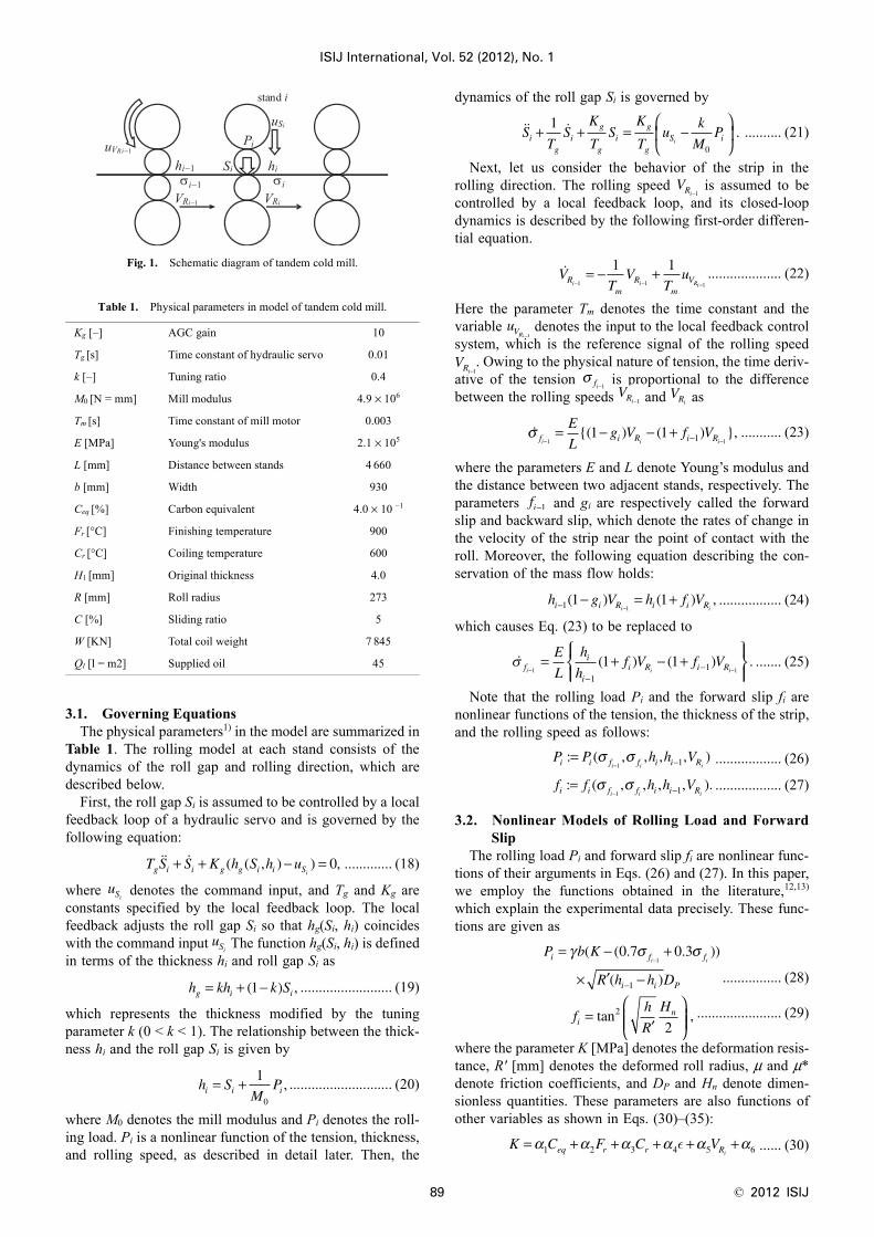
A tandem cold mill consists of several stands as shown inFig. 1. At stand i, the strip enters and exits the stand withthicknesses hi−1 and hi, respectively. The roll gap is denotedby Si and the rolling load is denoted by Pi . While the strippasses through stand i, the thickness hi and tension arecontrolled by adjusting the roll gap Si and rolling speed .

∈

u x t u t x t TRH( ( )) ( ; ( ), )*=

x tin*( )∈ λi

nt*( )∈ p timp*( )∈

u timu*( )∈ μi

mt c*( )∈

x t x t f x t u t p ti i i i i+ = +1* * * * *( ) ( ) ( ( ), ( ), ( ))Δτ

x t x t0*( ) ( )=

H x t t u t t p tu i i i i i( ( ), ( ), ( ), ( ), ( ))* * * * *λ μ+ =1 0

C x t u t p ti i i( ( ), ( ), ( ))* * * = 0

λ λ

λ μi i

x i i i i i

t t

H x t t u t t p t

* *

* * * * *

( ) ( )

( ( ), ( ), ( ), ( ), ( ))

=

++

+

1

1T Δττλ φN x N Nt x t p t* * *( ) ( ( ), ( )),= T

H x u p L x u p f x u p

C x u p

( , , , , ) : ( , , ) ( , , )

( , , ),

λ μ λμ

= +

+

T

T

x ti*( ) λi t

*( ) u ti*( )

μi t*( )

x t0*( )

U t mN( )∈ u ti*( )

μi t*( )

U t u t t u t tN N( ) : [ ( ) ( ) ( ) ( )] ,* * * *= − −0 0 1 1T T T T Tμ μ

x ti*( ) λi t

*( )

x ti*( )

λi t*( )

F U t x t t

H x t t u t t p t

C x

u

( ( ), ( ), )

:

( ( ), ( ), ( ), ( ), ( ))

(

* * * * *

=

T0 1 0 0 0λ μ

00 0 0

1 1 1

* * *

* * * *

( ), ( ), ( ))

( ( ), ( ), ( ), (

t u t p t

H x t t u t tu N N N NT

− − −λ μ )), ( ))

( ( ), ( ), ( ))

*

* * *

p t

C x t u t p t

N

N N N

−

− − −

⎡

⎣

⎢⎢⎢⎢⎢⎢⎢

⎤

⎦

⎥⎥⎥⎥⎥⎥1

1 1 1 ⎥⎥

= 0

mN mu→

u t P U t u t( ) ( ( )) : ( )*= =0 0

F U x( ( ), ( ), )0 0 0 0=

F U t x t t F U t x t t( ( ), ( ), ) ( ( ), ( ), )= −ζ

ζ > 0U t( )

F U F F x FU x t= − − −ζU t( ) U t( )

U t( )

σ fi−1

VRi−1


89 © 2012 ISIJ

3.1. Governing EquationsThe physical parameters1) in the model are summarized in

Table 1. The rolling model at each stand consists of thedynamics of the roll gap and rolling direction, which aredescribed below.

First, the roll gap Si is assumed to be controlled by a localfeedback loop of a hydraulic servo and is governed by thefollowing equation:

............. (18)

where denotes the command input, and Tg and Kg areconstants specified by the local feedback loop. The localfeedback adjusts the roll gap Si so that hg(Si, hi) coincideswith the command input The function hg(Si, hi) is definedin terms of the thickness hi and roll gap Si as

......................... (19)

which represents the thickness modified by the tuningparameter k (0 < k < 1). The relationship between the thick-ness hi and the roll gap Si is given by

............................ (20)

where M0 denotes the mill modulus and Pi denotes the roll-ing load. Pi is a nonlinear function of the tension, thickness,and rolling speed, as described in detail later. Then, the

dynamics of the roll gap Si is governed by

.......... (21)

Next, let us consider the behavior of the strip in therolling direction. The rolling speed is assumed to becontrolled by a local feedback loop, and its closed-loopdynamics is described by the following first-order differen-tial equation.

.................... (22)

Here the parameter Tm denotes the time constant and thevariable denotes the input to the local feedback controlsystem, which is the reference signal of the rolling speed

. Owing to the physical nature of tension, the time deriv-ative of the tension is proportional to the differencebetween the rolling speeds and as

........... (23)

where the parameters E and L denote Young’s modulus andthe distance between two adjacent stands, respectively. Theparameters and gi are respectively called the forwardslip and backward slip, which denote the rates of change inthe velocity of the strip near the point of contact with theroll. Moreover, the following equation describing the con-servation of the mass flow holds:

................. (24)

which causes Eq. (23) to be replaced to

....... (25)

Note that the rolling load Pi and the forward slip fi arenonlinear functions of the tension, the thickness of the strip,and the rolling speed as follows:

.................. (26)

.................. (27)

3.2. Nonlinear Models of Rolling Load and ForwardSlip

The rolling load Pi and forward slip fi are nonlinear func-tions of their arguments in Eqs. (26) and (27). In this paper,we employ the functions obtained in the literature,12,13)

which explain the experimental data precisely. These func-tions are given as

................ (28)

....................... (29)

where the parameter K [MPa] denotes the deformation resis-tance, R′ [mm] denotes the deformed roll radius, μ and μ*denote friction coefficients, and DP and Hn denote dimen-sionless quantities. These parameters are also functions ofother variables as shown in Eqs. (30)–(35):

...... (30)

Fig. 1. Schematic diagram of tandem cold mill.

Table 1. Physical parameters in model of tandem cold mill.

Kg [–] AGC gain 10

Tg [s] Time constant of hydraulic servo 0.01

k [–] Tuning ratio 0.4

M0 [N = mm] Mill modulus 4.9 × 106

Tm [s] Time constant of mill motor 0.003

E [MPa] Young's modulus 2.1 × 105

L [mm] Distance between stands 4 660

b [mm] Width 930

Ceq [%] Carbon equivalent 4.0 × 10 −1

Fr [°C] Finishing temperature 900

Cr [°C] Coiling temperature 600

H1 [mm] Original thickness 4.0

R [mm] Roll radius 273

C [%] Sliding ratio 5

W [KN] Total coil weight 7 845

Ql [l = m2] Supplied oil 45

T S S K h S h ug i i g g i i Si+ + − =( ( , ) ) ,0

uSi

uSi

h kh k Sg i i= + −( ) ,1

h SM

Pi i i= + 1

0

,

STS

K

TS

K

Tu

k

MPi

gi

g

gi

g

gS ii

+ + = −⎛

⎝⎜

⎞

⎠⎟

1

0

.

VRi−1

VTV

TuR

mR

mVi i Ri− − −

= − +1 1 1

1 1

uVRi−1

VRi−1 σ fi−1VRi−1 VRi

σ f i R i Ri i i

E

Lg V f V

− −= − − + −1 1

1 1 1{( ) ( ) },

fi−1

h g V h f Vi i R i i Ri i− − = +−1 1 11

( ) ( ) ,

σ fi

ii R i Ri i i

E

L

h

hf V f V

− −= + − +

⎧⎨⎪

⎩⎪

⎫⎬⎪

⎭⎪−−1 1

111 1( ) ( ) .

P P h h Vi i f f i i Ri i i: ( , , , , )=

− −σ σ1 1

f f h h Vi i f f i i Ri i i: ( , , , , ).=

− −σ σ1 1

P b K

R h h D

i f f

i i P

i i= − +

× ′ −−

−

γ σ σ( ( . . ))

( )

0 7 0 31

1

fh

R

Hi

n=′

⎛

⎝⎜⎜

⎞

⎠⎟⎟tan ,2

2

K C F C Veq r r Ri= + + + + +α α α α α α1 2 3 4 5 6ε

© 2012 ISIJ 90


............... (31)

.......... (32)

.... (33)

........... (34)

................... (35)

Here the logarithmic strain and the reduction in thickness,r, are defined as

............................... (36)

.............................. (37)

Note that Eqs. (30) and (34) involve the rolling speed .Although the exact value of is obtained by solving Eqs.(28) and (31), an approximate solution 1.2R is adoptedhere owing to the difficulty of finding the exact solution. Theparameters in the above equations are summarized in Table 2.

3.3. State EquationThe state equation for stand i is now constructed in accor-

dance with the previous subsections. The state vector x andinput vector u are defined as

......... (38)

................... (39)

Then, the state equation of this system is expressed as

...... (40)

............... (41)

........... (42)

3.4. Expression of ThicknessThe thickness hi is a function of the state as shown in Eq.

(20). However, it is difficult to express the thickness explic-itly from Eq. (20) because the rolling load Pi is also a func-tion of the thickness hi as in Eq. (26). In this study, we pro-pose an approximate expression for hi. Assuming that hi isalways controlled within the neighborhood of its desiredvalue , Eq. (20) can be approximated by

.... (43)

where and denotes a small deviation of thethickness from its desired value. This approximation givesan explicit expression for hi that depends on x and .

4. Application of RHC to a Tandem Cold Mill

4.1. RHC for Nonlinear ModelWe design RHC for the nonlinear model developed in the

previous section. A single stand (i = 1) is considered, andthe control objective is to keep the thickness and tensionconstant during changes in the rolling speed. Deviations ofthe thickness and tension from their reference values arepenalized in the performance index for RHC.

In the case of a single stand, the state vector is four-dimensional, , and the input vector istwo-dimensional, . The entry thickness andentry tension are denoted by h0 and , respectively, and areassumed to be constant. The strip is accelerated or deceler-ated in accordance with a given profile for the rolling speed

.

4.1.1. Performance IndexFirst, the thickness h1 is obtained explicitly from the

approximation given by Eq. (43) as a function of the state,i.e., h1 = h1(x). Moreover, the desired state and corre-sponding desired input are assumed to be obtainedappropriately. Then, the performance index is defined topenalize deviations of the state and input from their desiredvalues as

Table 2. Parameters in nonlinear model of P and f.

α1 [MPa/%] 9.752 × 10+3

α2 [MPa/°C] –4.206 × 10−1

α3 [MPa/°C] 2.227 × 10−2

α4 [MPa] 2.226 × 10+2

α5 [MPa·s/mm] 9.864 × 10−4

α6 [MPa] 8.385 × 10+2

AV [–] –1.69 × 10−3

AW [–] 1.443 × 10−2

AQ [–] 6.88 × 10−3

Ar [–] –6.2 × 10−3

AH [/mm] –4.112 × 10−2

Ah [/mm] 5.148 × 10−2

Ab [/MPa] 2.43 × 10−5

Af [/MPa] –6.94 × 10−6

AK [/MPa] –6.04 × 10−5

A0 [–] 4.049 × 10−2

BV [s/mm] –4.637 × 10−5

BW [/KN] –4.24 × 10−5

BQ [m2/l] –2.990 × 10−2

′ = +−

⎛

⎝⎜

⎞

⎠⎟ ≅

−

R R cP

b h hR

i i

1 1 21( )

.

D r rR

hrp

i

= + −′−1 08 1 79 1 1 02. . .μ

μ μ=− −

− − −

−−

−

−−

−

tan ( / ) tan

tan ( / ) tan

(

*1

11

11

1

1 2

1 2

h h f

h h f C

f

i i i

i i s

ss i i if f C C f C= ≥ <( ), ( ))

μ

σ

σ

* · · ·= + +

+ + + +

+− −

A e A e A e

A r A h A h A

A

V

B V

WB W

QB Q

r H i h i b f

f f

V Ri W Q l

i1 1

iiA K AK+ + 0

HR

h

h

h

h K

h K

ni

i

i

i f

i f

i

i

=′

−

−−−

− −

−

−

tan

ln( )

( ).

*

1 1

1

1

1

21

μ

σ

σ

ε

ε = − ln h

Hi

1

rh h

hi i

i

= −−

−

1

1

.

VRi′R

′ ≅R

x x x x x S S Vi i f Ri i= =

− −[ , , , ] : [ , , , ]1 2 3 4 1 1

T Tσ

u u u u uS Vi Ri= =

−[ , ] : [ , ] .1 2

1

T T

x

x

f

f

T x

K T

Tm

g g

m

=

−

⎡

⎣

⎢⎢⎢⎢

⎤

⎦

⎥⎥⎥⎥+

⎡

⎣

⎢⎢⎢⎢⎢

⎤

⎦

2

2

3

41

0 0

0

0 0

0 1

,

,

,

( / )

/

/

⎥⎥⎥⎥⎥⎥

⎡

⎣⎢⎢

⎤

⎦⎥⎥

−

u

u

S

V

i

Ri 1

fK

Tx

Tx

K

T

k

MPg

g g

g

gi2 1 2

0

1= − − −

fE

L

h

hf V f xi

ii R ii3

11 41 1= + − +

⎧⎨⎩

⎫⎬⎭−

−( ) ( ) .

hir

h hP x h h V M h S

M P hi ir i f i

ri R i

ri

i i h h

i i

i i

≈ +− −

− ∂ ∂−

=

( , , , , ) ( )

( / )3 1 0

0

σ

rr

,

h h hi ir

i= + Δ Δhi

hr

x S S Vf R= [ , , , ]1 1 0 0σ T

u u uS VR= [ , ]

1 0

T

σ f1

VR1

x tr ( )u tr ( )


91 © 2012 ISIJ

.......... (44)

where and denote the deviation of thestate from the desired state and the deviation of the inputfrom the desired input, respectively, and ,

, and are positive-definite weightingmatrices. In this paper, the thickness h1 itself is not includedin the performance index to avoid a complicated perfor-mance index. Instead, the desired state is defined so as toachieve the desired thickness and desired tension, and theperformance index is defined for the actual state to track thedesired state. As a result, the tracking of the desired valuesof the thickness and tension is achieved indirectly by mini-mizing the performance index given by Eq. (44).

4.1.2. Desired StateThe desired state and corresponding desired input are

required in order to obtain the performance index given byEq. (44). They depend on the rolling speed and, there-fore, are functions of time. Since and h1 are to bekept constant, the desired state xr and desired input ur mustsatisfy

............................. (45)

for constant and h1. The desired constant values of and and as a function of time are assumed to be

given, and and h0 are also assumed to be given constants.Therefore, , , and are quantities to be deter-mined at each time.

First, is determined from the third element of Eq.(45). That is,

............ (46)

Since is constant, and = 0 and f0 = 0 hold identically,we have

....................... (47)

which gives as

......................... (48)

Then, is obtained by differentiating Eq. (48) with respectto time as

............ (49)

Next, is determined as follows. Although thethickness hi is determined approximately by Eq. (43), Eq.(43) is equivalent to Eq. (20) when holds. Therefore,Eq. (20) gives as

............... (50)

The time derivative is obtained by differentiatingEq. (50) with respect to time as

............... (51)

Note that only is time-varying among the arguments ofP1. Furthermore, is obtained by differentiating Eq.(51) with respect to time as

.............. (52)

Finally, the desired input to achieve the desired state isdetermined from the second and fourth elements of Eq. (45)as follows.

.................. (53)

......................... (54)

As shown by Eqs. (52) and (53), it is necessary to specifythe values of and its derivatives and to determinethe desired values of the state and input.

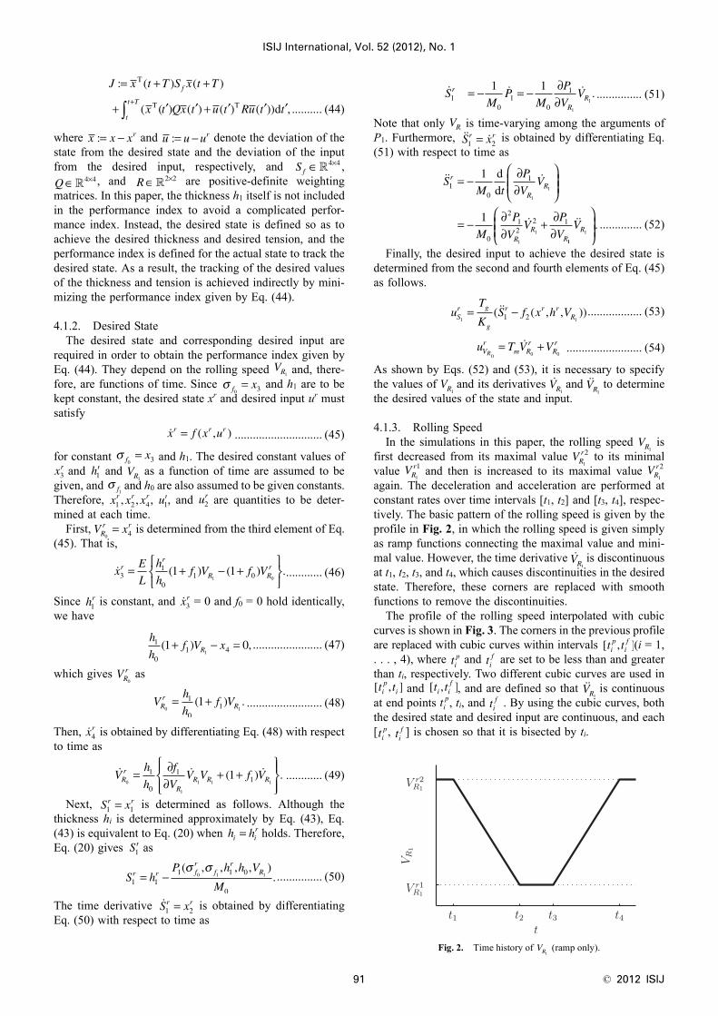
4.1.3. Rolling SpeedIn the simulations in this paper, the rolling speed is

first decreased from its maximal value to its minimalvalue and then is increased to its maximal value again. The deceleration and acceleration are performed atconstant rates over time intervals [t1, t2] and [t3, t4], respec-tively. The basic pattern of the rolling speed is given by theprofile in Fig. 2, in which the rolling speed is given simplyas ramp functions connecting the maximal value and mini-mal value. However, the time derivative is discontinuousat t1, t2, t3, and t4, which causes discontinuities in the desiredstate. Therefore, these corners are replaced with smoothfunctions to remove the discontinuities.

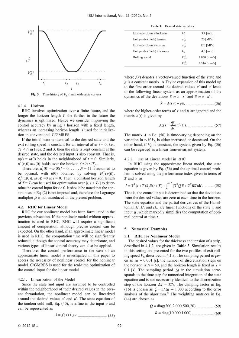
The profile of the rolling speed interpolated with cubiccurves is shown in Fig. 3. The corners in the previous profileare replaced with cubic curves within intervals (i = 1,. . . , 4), where and are set to be less than and greaterthan ti, respectively. Two different cubic curves are used in

and , and are defined so that is continuousat end points , ti, and . By using the cubic curves, boththe desired state and desired input are continuous, and each[ , ] is chosen so that it is bisected by ti.

J x t T S x t T

x t Qx t u t Ru t t

f

t

t T

: ( ) ( )

( ( ) ( ) ( ) ( )) ,

= + +

+ ′ ′ + ′ ′ ′+

∫

T

T T d

x x xr:= − u u ur:= −

S f ∈×4 4

Q∈ ×4 4 R∈ ×2 2

VR1σ f x

0 3=

x f x ur r r= ( , )

σ f x0 3=

xr3 hr1 VR1σ f1

x x xr r r1 2 4, , ur1 ur2

V xRr r

0 4=

xE

L

h

hf V f Vr

r

R Rr

31

01 01 1

1 0= + − +

⎧⎨⎩

⎫⎬⎭

( ) ( ) .

hr1 xr3

h

hf V xR

1

01 41 0

1( ) ,+ − =

VRr

0

Vh

hf VR

rR0 1

1

011= +( ) .

xr4

Vh

h

f

VV V f VR

r

RR R R0

1

1 1 1

1

0

111= ∂

∂+ +

⎧⎨⎪

⎩⎪

⎫⎬⎪

⎭⎪( ) .

S xr r1 1=

h hi ir=

Sr1

S hP h h V

Mr r f

rf

rR

1 11 1 0

0

0 1 1= −( , , , , )

.σ σ

S xr r1 2=

Fig. 2. Time history of (ramp only).

SM

PM

P

VVr

RR1

01

0

11 1

1

1= − = − ∂

∂.

VR1S xr r1 2=

SM t

P

VV

M

P

VV

P

V

r

RR

RR

R

10

1

0

212

2 1

1

1

1

1

1

1

= − ∂∂

⎛

⎝⎜⎜

⎞

⎠⎟⎟

= − ∂∂

+ ∂∂

d

d

11

1VR

⎛

⎝⎜⎜

⎞

⎠⎟⎟.

uT

KS f x h VS

r g

g

r r rR1 11 2= −( ( , , ))

u T V VVr

m Rr

Rr

R0 0 0= +

VR1 VR1 VR1

VR1VRr

1

2

VRr

1

1 VRr

1

2

VR1

[ , ]t tip

if

tip ti

f

[ , ]t tip

i [ , ]t ti if

VR1tip ti

f

tip ti

f

VR1

© 2012 ISIJ 92


4.1.4. HorizonRHC involves optimization over a finite future, and the

longer the horizon length T, the further in the future thedynamics is optimized. Hence we consider improving thecontrol accuracy by using a horizon with a fixed length,whereas an increasing horizon length is used for initializa-tion in conventional C/GMRES.

If the initial state is identical to the desired state and theexit rolling speed is constant for an interval after t = 0, i.e.,Tf < t1 in Figs. 2 and 3, then the state is kept constant at thedesired state, and the desired input is also constant. That is,u(t) = u(0) holds in the neighborhood of t = 0. Similarly,

holds over the horizon .Therefore, (i = 0, . . . , N − 1) is assumed to

be optimal, with u(0) obtained by solving ,, u(0)) =0 at t = 0. Then, a constant horizon length

of T = Tf can be used for optimization over [t, t + Tf ] to deter-mine the control input for t > 0. It should be noted that the con-straint as in Eq. (2) is not imposed and, therefore, the Lagrangemultiplier μ is not introduced in the present problem.

4.2. RHC for Linear ModelRHC for our nonlinear model has been formulated in the

previous subsection. If the nonlinear model without approx-imation is used in RHC, RHC will require a significantamount of computation, although precise control can beexpected. On the other hand, if an approximate linear modelis used in RHC, the computation time will be significantlyreduced, although the control accuracy may deteriorate, andvarious types of linear control theory can also be applied.

Therefore, the control performance in the case of anapproximate linear model is investigated in this paper toaccess the necessity of nonlinear control for the nonlinearmodel. C/GMRES is used for the real-time optimization ofthe control input for the linear model.

4.2.1. Linearization of the ModelSince the state and input are assumed to be controlled

within the neighborhood of their desired values in the pres-ent formulation, the nonlinear model can be linearizedaround the desired values and . The state equation ofthe tandem cold mill, Eq. (40), is affine in the input u andcan be represented as

............................. (55)

where f(x) denotes a vector-valued function of the state andg is a constant matrix. A Taylor expansion of this model upto the first order around the desired values and leadsto the following linear system as an approximation of thedynamics of the deviations and :

............................ (56)

where the higher-order terms of and are ignored and thematrix A(t) is given by

.......................... (57)

The matrix A in Eq. (56) is time-varying depending on thevariation in xr if is either increased or decreased. On theother hand, if is constant, the system given by Eq. (56)can be regarded as a linear time-invariant system.

4.2.2. Use of Linear Model in RHCIn RHC using the approximate linear model, the state

equation is given by Eq. (56) and the optimal control prob-lem is solved using the performance index given in terms of

and as

......... (58)

That is, the control input is determined so that the deviationsfrom the desired values are zero at each time in the horizon.The state equation and the partial derivatives of the Hamil-tonian H, Hx and Hu, are linear functions of the state andinput , which markedly simplifies the computation of opti-mal control at time t.

5. Numerical Examples

5.1. RHC for Nonlinear ModelThe desired values for the thickness and tension of a strip,

described in 4.1.2, are given in Table 3. Simulation resultsin this setting are presented for the two profiles of exit roll-ing speed described in 4.1.3. The sampling period is giv-en as = 0.001 [s], the number of discretization steps onthe horizon is N = 50, and the horizon length is fixed as T =0.1 [s]. The sampling period in the simulation corre-sponds to the time step for numerical integration of the stateequation and is not necessarily identical to the discretizationstep of the horizon = T/N. The damping factor in Eq.(16) is chosen as = 1 000 according to the erroranalysis of the algorithm.6) The weighting matrices in Eq.(44) are chosen as

................. (59)

...................... (60)

Fig. 3. Time history of (ramp with cubic curves).VR1

u u*( , ) ( )τ 0 0= 0 ≤ ≤τ Tfu ui*( ) ( )0 0=

H xuT ( ( )0

φx xT ( ( ))0

xr ur

x f x gu= +( ) ,

Table 3. Desired state variables.

Exit-side (Front) thickness h r1 3.4 [mm]

Entry-side (Back) tension σ rf0 20 [MPa]

Exit-side (Front) tension σ rf1 120 [MPa]

Entry-side (Back) thickness h0 4.0 [mm]

Rolling speed V r1R1 1 050 [mm/s]

V r2R1 6 316 [mm/s]

xr ur

x x xr:= − u u ur:= −

x A t x gu= +( ) ,

x u

A tf

xx tr( ) : ( ( )).= ∂

∂

VR1VR1

x u

J x t T S x t T x Q x u Ru tf t

t T= + + + + ′

+

∫T T T( ) ( ) ( ) .d

xu

VR1Δt

Δt

Δτζ =1 / Δt

Q = diag( , , , )200 2 000 500 20

R = diag( , )10 000 1 000


93 © 2012 ISIJ

.................... (61)

The parameters for the two profiles of in 4.1.3 are giv-en as follows:

1. Ramp

2. Ramp and cubic curves, and cubic curves are used

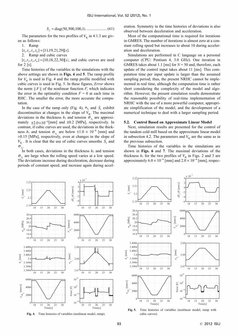
for 2 [s].Time histories of the variables in the simulations with the

above settings are shown in Figs. 4 and 5. The ramp profilefor is used in Fig. 4 and the ramp profile modified withcubic curves is used in Fig. 5. In these figures, Error showsthe norm of the nonlinear function F, which indicatesthe error in the optimality condition F = 0 at each time inRHC. The smaller the error, the more accurate the compu-tation.

In the case of the ramp only (Fig. 4), and exhibitdiscontinuities at changes in the slope of . The maximaldeviations in the thickness h1 and tension are approxi-mately [mm] and ±0.2 [MPa], respectively. Incontrast, if cubic curves are used, the deviations in the thick-ness h1 and tension are below ±1.0 × 10−4 [mm] and±0.15 [MPa], respectively, even at changes in the slope of

. It is clear that the use of cubic curves smooths and.

In both cases, deviations in the thickness h1 and tension are large when the rolling speed varies at a low speed.

The deviations increase during deceleration, decrease duringperiods of constant speed, and increase again during accel-

eration. Symmetry in the time histories of deviations is alsoobserved between deceleration and acceleration.

Most of the computational time is required for iterationsin GMRES. The number of iterations is almost zero at a con-stant rolling speed but increases to about 10 during acceler-ation and deceleration.

Simulations are performed in C language on a personalcomputer (CPU: Pentium 4, 3.0 GHz). One iteration inGMRES takes about 1.1 [ms] for N = 50 and, therefore, eachupdate of the control input takes about 11 [ms]. This com-putation time per input update is larger than the assumedsampling period; thus, the present NRHC cannot be imple-mented in real time, although the computation time is rathershort considering the complexity of the model and algo-rithm. However, the present simulation results demonstratethe reasonable possibility of real-time implementation ofNRHC with the use of a more powerful computer, appropri-ate simplification of the model, and the development of anumerical technique to deal with a larger sampling period.

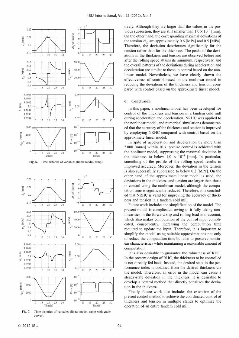
5.2. Control Based on Approximate Linear ModelNext, simulation results are presented for the control of

the tandem cold mill based on the approximate linear modelin subsection 4.2. The parameters and are the same as inthe previous subsection.

Time histories of the variables in the simulations areshown in Figs. 6 and 7. The maximal deviations of thethickness h1 for the two profiles of in Figs. 2 and 3 areapproximately 6.0 × 10−4 [mm] and 2.0 × 10−4 [mm], respec-

Fig. 4. Time histories of variables (nonlinear model, ramp).

S f = diag( , , , ).50 500 100 1

VR1

[ , , , ] [ , , , ][ ].t t t t s1 2 3 4 11 19 21 29=

[ , , , ] [ , , , ][ ]t t t t s1 2 3 4 10 18 22 30=

VR1

F

uS1 S1VR1σ f0

± × −2 0 10 4.

σ f0

VR1 S1σ f0

σ f0

Fig. 5. Time histories of variables (nonlinear model, ramp withcubic curves).

VR1

VR1

© 2012 ISIJ 94


tively. Although they are larger than the values in the pre-vious subsection, they are still smaller than 1.0 × 10−3 [mm].On the other hand, the corresponding maximal deviations ofthe tension are approximately 0.6 [MPa] and 0.5 [MPa].Therefore, the deviation deteriorates significantly for thetension rather than for the thickness. The peaks of the devi-ations in the thickness and tension are observed before andafter the rolling speed attains its minimum, respectively, andthe overall patterns of the deviations during acceleration anddeceleration are similar to those in control based on the non-linear model. Nevertheless, we have clearly shown theeffectiveness of control based on the nonlinear model inreducing the deviations of the thickness and tension, com-pared with control based on the approximate linear model.

6. Conclusion

In this paper, a nonlinear model has been developed forcontrol of the thickness and tension in a tandem cold millduring acceleration and deceleration. NRHC was applied tothe nonlinear model, and numerical simulations demonstrat-ed that the accuracy of the thickness and tension is improvedby employing NRHC compared with control based on theapproximate linear model.

In spite of acceleration and deceleration by more than5 000 [mm/s] within 10 s, precise control is achieved withthe nonlinear model, suppressing the maximal deviation inthe thickness to below 1.0 × 10−4 [mm]. In particular,smoothing of the profile of the rolling speed results inimproved accuracy. Moreover, the deviation in the tensionis also successfully suppressed to below 0.2 [MPa]. On theother hand, if the approximate linear model is used, thedeviations in the thickness and tension are larger than thosein control using the nonlinear model, although the compu-tation time is significantly reduced. Therefore, it is conclud-ed that NRHC is valid for improving the accuracy of thick-ness and tension in a tandem cold mill.

Future work includes the simplification of the model. Thepresent model is complicated owing to it fully taking non-linearities in the forward slip and rolling load into account,which also makes computation of the control input compli-cated, consequently, increasing the computation timerequired to update the input. Therefore, it is important tosimplify the model using suitable approximations not onlyto reduce the computation time but also to preserve nonlin-ear characteristics while maintaining a reasonable amount ofcomputation.

It is also desirable to guarantee the robustness of RHC.In the present design of RHC, the thickness to be controlledis not directly fed back. Instead, the desired state in the per-formance index is obtained from the desired thickness viathe model. Therefore, an error in the model can cause asteady-state deviation in the thickness. It is desirable todevelop a control method that directly penalizes the devia-tion in the thickness.

Finally, future work also includes the extension of thepresent control method to achieve the coordinated control ofthickness and tension in multiple stands to optimize theoperation of an entire tandem cold mill.

Fig. 6. Time histories of variables (linear model, ramp).

Fig. 7. Time histories of variables (linear model, ramp with cubiccurves).

σ f0


95 © 2012 ISIJ

AcknowledgmentThis work was carried out as part of the Research Group

on Novel Steel Process Control based on On-Line Optimi-zation Technology, which was part of the Division of Instru-mentation, Control and System Engineering, the Iron andSteel Institute of Japan. This work was also partly supportedby Grant-in-Aid for Scientific Research (C) 21560465 fromthe Japan Society for the Promotion of Science.

REFERENCES

1) A. Kitamura, M. Konishi and Y. Naito: Trans. Inst. Syst., Control Inf.Eng., 4 (1991), 140.

2) T. Ooi, F. Nishimura, T. Yanagita, S. Ban and Y. Seki: Trans. Inst.Syst., Control Inf. Eng., 9 (1996), 274.

3) Y. Asada, A. Kitamura, M. Konishi, T. Morita and H. Akedo: Tetsu-

to-Hagané, 67 (1981), 2551.4) A. Kojima and T. Ohtsuka: J. Soc. Instrum. Control Eng., 42 (2003),

310.5) T. Ohtsuka: J. Soc. Instrum. Control Eng., 41 (2002), 366.6) T. Ohtsuka: Automatica, 40 (2004), 563.7) H. Seguchi and T. Ohtsuka: Int. J. Robust Nonlinear Control, 13

(2003), 381.8) M. Hamamatsu, H. Kagaya and Y. Kohno: Trans. Soc. Instrum. Con-

trol Eng., 44 (2008), 685.9) M. Nagatsuka, N. Shishido, K. Masui and H. Tomita: Prof. of 44th

Aircraft Symp., JSASS, Tokyo, (2006), 201.10) A. E. Bryson, Jr. and Y.-C. Ho: Applied Optimal Control, Hemi-

sphere, New York, (1975).11) C. T. Kelley: Iterative Methods for Linear and Nonlinear Equations,

SIAM, Philadelphia, (1995).12) Y. Misaka: J. Jpn. Soc. Technol. Plast., 8 (1967), 188.13) T. Shiraishi, H. Yamamoto, J. Hashimoto and T. Niitome: J. Jpn. Soc.

Technol. Plast., 36 (1995), 1269.

Documents

Nonlinear Receding Horizon Control of Thickness and