Receding Horizon Control of an SIS Epidemic: Optimality and Asymptotic ...web.cs.elte.hu/blobs/diplomamunkak/msc_mat/2014/selley_fanni.pdf · an SIS Epidemic: Optimality and Asymptotic

Receding Horizon Control of

an SIS Epidemic: Optimality

and Asymptotic Stability

Fanni SelleyMSc in Pure Mathemathics

Supervisor: Adam Besenyei

Department of Applied Analysis and Computational Mathematics

Eotvos Lorand University Faculty of Science

Master’s Thesis

2014

mailto:[email protected]

mailto:[email protected]

http://www.cs.elte.hu/applanal/eng/index_eng.html

http://ttk.elte.hu

ii

Koszonetnyilvanıtas

Koszonettel tartozom temavezetomnek, Besenyei Adamnak minden segıt-

segeert es a velem szemben tanusıtott turelmeert az elmult ket evben. Szin-

ten koszonettel tartozom Simon Peternek tamogatasaert es iranymutatasa-

ert, hiszen az o vezetese alatt indulhatott el a munkam a szakdolgozatom

temajaban. Koszonom Gyurkovics Evanak a tanulsagos konzultaciokat es a

munkam iranyanak kijeloleset. Koszonom Kovacs Balazsnak es Mincsovics

Miklosnak a hasznos megjegyzeseiket es javaslataikat. Vegezetul koszonettel

tartozom a csaladomnak bizalmukert es tamogatasukert.

ii

Contents

1 Introduction 1

2 Formulation of the Control Problem 3

2.1 SIS Epidemic Models . . . . . . . . . . . . . . . . . . . . . . . . . . . . . 3

2.2 Controlling the Epidemic: the Basic Idea . . . . . . . . . . . . . . . . . 6

2.3 Brief Overview of Receding Horizon Control . . . . . . . . . . . . . . . . 8

2.4 Optimal Control of our Epidemic Model . . . . . . . . . . . . . . . . . . 11

3 Stability Analysis 15

3.1 Asymptotic Stability of Hε in the Exact Discrete Model . . . . . . . . . 16

3.2 Asymptotic Stability of Hε in the Approximative Discrete Model . . . . 22

4 Simulation Results 27

4.1 Results . . . . . . . . . . . . . . . . . . . . . . . . . . . . . . . . . . . . . 29

4.1.1 Tests for Various Parameters . . . . . . . . . . . . . . . . . . . . 29

4.1.2 Advantages to Constant Control . . . . . . . . . . . . . . . . . . 32

4.1.3 An Alternative Cost Functional . . . . . . . . . . . . . . . . . . . 36

5 Discussion 39

A Matlab Software 41

Bibliography 47

iii

CONTENTS

iv

1

Introduction

Being able to control a process or a complex system has always been a question of great

interest and subject of extensive research. Control theory on its own has grown out to

be a significant branch of mathematics but still managed to stay widely applicable in

engineering, biology and medicine.

Mathemathical models of disease transmisson are generally developed to enable us

to give predicitions about the outcome of the epidemic and our capability of controlling

the outbreak. A carefully designed model can give important insight into understanding

which actions have to be taken to reduce the prevalence of the infection or eradicate it

completely. For many models, this is well understood when control such as vaccination

(see for example Anderson [1]), quarantine or contact tracing (see Kiss [13]) is consid-

ered. However, in most epidemic control models a classic compartmental type model

is considered and the control does not form an integral part of the disease dynamics.

The model we propose in this thesis is based on a more modern approach. We con-

sider a network-based epidemic model describing a susceptible-infectious-susceptible

(SIS) epidemic on a non-trivial contact structure. We propose a control by altering the

contact network within the population. Our method, based on the algorithm of Reced-

ing Horizon Control, operates with tools similar to quarantining but it is less radical

though still effective. The stability and suboptimality analysis of receding horizon-type

control algorithms has been an active topic of research in the last decades, we will apply

some results to better understand the nature of our control.

In Chapter 2 of this thesis we first give a brief overview of some mathemathical

tools of epidemiology and control theory, then we precisely formulate the control prob-

1

1. INTRODUCTION

lem. We will also briefly discuss the suboptimality of our control strategy. In Chapter

3 we analyze the stability properties of our control. Finally, in Chapter 4 we give a

thorough and extensive numerical investigation of the impact of the infection parame-

ters (infection rate, recovery rate) and control parameters on the nature of the control

computed. The numerical tests were conducted in Matlab R2011a, the codes are given

in Appendix A.

2

2

Formulation of the Control

Problem

In this section we will give an overview of two well-known mathemathical modesl of

epidemic spreading and control theory. After familiarizing ourselves with these models

we formulate our control problem by combining them.

2.1 SIS Epidemic Models

The beginning of mathemathical modelling of epidemics dates back to the classic article

[12] by A. G. McKendrick and W. O. Kermack. They constructed a relatively simple

model where each individual of the population is assigned to one of two compartments,

the class of infectious and the class of susceptible individuals. The dynamics of infection

is described by a single differential equation based on simple heuristics. Since their

pioneering work this area of mathematics has gained massive popularity and today

many sophisticated models exist, we refer to the excellent textbooks of Diekmann and

Hesterbreek [4], Anderson and May [1] and Keeling and Rohani [11].

Let us first introduce the abstract mathematical setting of epidemic modelling.

Representing the social network of the population, consider an undirected simple graph

with N nodes and a finite set of states {a1, . . . , am}. Each node could be in any of

these states at each time instant, so the number of possible states of the graph is mN .

Nodes change their states according to a Poisson process: the probability of each node

changing its state from ai to aj during a time interval of length ∆t is 1− exp(−λij∆t),

3

2. FORMULATION OF THE CONTROL PROBLEM

where we call the parameter λij > 0 transmission rate. Naturally these parameters

depend on the states of the node’s neighbours. So the mathematical structure we are

dealing with is a continuous-time Markov chain on a state space of size mN , whose

state equation is a set of mN linear differential equations.

In our work we will consider an SIS model, where SIS is short for Susceptible-

Infectious-Susceptible. This means that we have two states, each individual could be

either susceptible or infectious. We will denote these states as S and I, respectively. A

susceptible individual can become infectious when contacted with an infectious one, and

an infectious one can recover and become susceptible again after some time has passed.

So we consider a simple, non-lethal infection where gaining immunity is impossible.

Both infection and recovery is governed by a Poisson process: if a node in state S has k

neighbours in state I, then the probabilty of becoming infectious during a time interval

of ∆t is 1 − exp(−kτ∆t) and a node in state I recovers during a time interval of ∆t

with the probability of 1− exp(−γ∆t). The parameters τ > 0 and γ > 0 are called the

infection rate and the recovery rate.

Remark 2.1. We would like to strongly emphasize that our goal in this work is not to

describe an actual epidemic, rather to understand and analyze the qualitative properties

of the mathemathical model given above.

We will now define a set of differential equations modelling the dynamics of the

stochastic process just described. Consider the following functions of t: [I](·), [SI](·),[II](·) and [SS](·) where I denotes the number of infectious individuals at time t,

SI denotes the number of susceptible-infectious connections, II denotes the number

of infectious-infectious connections, SS denotes the number of susceptible-susceptible

connections and [·] marks the expected value. Since it causes no confusion, we will

omit the variable t from now on. Our main interest is [I], for which we can give the

following differential equation by the Poisson processes discussed above:

[I] = τ [SI]− γ[I].

This equation formalizes that the change in the expected value of the infectious indi-

viduals is a consequence of either infection or recovery: the existing number of S − Iconnections influences positively the rate of change with a rate of τ and the number of I

influences it negatively with a rate of γ. Clearly, this is not a self-contained differential

4

2.1 SIS Epidemic Models

equation, we need a differential equation for [SI] to close the system. This leads to

further equations and finally we obtain the system

˙[I] = τ [SI]− γ[I], (2.1a)

˙[SI] = γ([II]− [SI]) + τ([SSI]− [ISI]− [SI]), (2.1b)

˙[II] = −2γ[II] + 2τ([ISI] + [SI]), (2.1c)

˙[SS] = 2γ[SI]− 2τ [SSI], (2.1d)

which holds for an arbitrary graph (for proof see [15]). In system (2.1a)–(2.1d), [SSI]

and [ISI] stands for the expected value of S−S− I and I −S− I triples, respectively.

These triples need not be complete subgraphs, they should only be connected: so either

triangles or paths of length three. We see that our system is still not self-contained,

but one can give a fairly good approximation for the expected value of these triples

using a type of moment closure formula (see [10], [16]). Let n be the (expected) mean

degree of the graph, then

[SSI] ' n− 1

n

[SS][SI]

N − [I]and [ISI] ' n− 1

n

[SI]2

N − [I]

will be substituted in system (2.1a)–(2.1d). As n we denoted the mean degree of the

graph, defined as the double of the (expected) number of edges divided by the number

of nodes:

n =2 · [SI] + [II] + [SS]

N.

The moment closure formulas can be explained heuristically in the following way: take

the first one for example, and let us denote N − [I] = [S]. A node in state S has

approximately n neighbours. The number of susceptible nodes on the average is [S],

so n[S] edges start from the set of susceptible nodes. The number of SI edges on the

average is [SI], so an edge from a randomly chosen node in state S ends in a node in

state I with the probability of [SI]/n[S]. So from the n edges connected to a node

in state S approximately n[SI]/n[S] = [SI]/[S] are of type SI. Similarly, from the

remaining n− 1 edges a portion of [SS]/n[S] edges end in another node in state S. So

the number os SSI triples where the middle node is a fixed node in state S is

[SI]

[S](n− 1)

[SS]

n[S].

5


This is true for every node in state S, so we have to multiply the above formula with

[S] to get the number of all SSI triples. We can argue similarly to get the formula for

[ISI].

When the moment closure formulas are substituted, we obtain the following system:

˙[I] = τ [SI]− γ[I], (2.2a)

˙[SI] = γ([II]− [SI]) + τ

(1− N

2 · [SI] + [II] + [SS]

)[SS][SI]

N − [I]

− τ(

1− N

2 · [SI] + [II] + [SS]

)[SI]2

N − [I]− τ [SI], (2.2b)

˙[II] = −2γ[II] + 2τ

((1− N

2 · [SI] + [II] + [SS]

)[SI]2

N − [I]+ [SI]

), (2.2c)

˙[SS] = 2γ[SI]− 2τ

(1− N

2 · [SI] + [II] + [SS]

)[SS][SI]

N − [I]. (2.2d)

The correctness of this system was tested by comparing it to Monte-Carlo simu-

lations in [15]. The results were agreeable in the sense that the expected number of

infectious individuals were sufficiently close when the computed value of the model

using the moment closure formulas and the average of 1000 simulations of the actual

Poisson processes were compared. So we can proceed working with this system knowing

that it gives a good approximation of the exact dynamics.

2.2 Controlling the Epidemic: the Basic Idea

Once we understand the dynamics of an epidemic, we would naturally like to control

it. By control we mean some kind of intervention in the dynamics of the model to

reach certain goals, such as keeping the expected number of infectious individuals or

infectious-susceptible connections under a predetermined threshold or at a target value

etc. Our primary goal in this work will be to eradicate the infection, so we would like

to have [I] = 0. To achieve this, we will not control the variable [I], but the variable

[SI]. The idea of our control scheme is to delete connections between infectious and

susceptible individuals. This decreases the value of [I], since if a node in state S has

fewer infectious neighbours, it is less likely to become infectious – the expected value

of the number of infectious individuals thus decreases.

Obviously, if we delete every infectious-susceptible connection (creating sort of a

quarantine), all infectious nodes will recover after a while and then our goal is reached.

6

2.2 Controlling the Epidemic: the Basic Idea

However, a control of this extent would be too radical, potentially isolating the popu-

lation. In our work we would also like to maintain the integrity of the social network

in some sense. Namely, we would like to keep the mean degree of the graph around a

desirable value, so our secondary goal will be to have n(t) = n∗ for sufficiently large

t ≥ 0 where n∗ is some desirable mean degree. To reach this, we have to create new

connections (since many were deleted), and creating susceptible-susceptible connections

is a good idea, since it is expected not to interfere with our primary goal much.

Now let us formalize the above heuristics. We will include two new functions in

our system (2.2a)–(2.2d), u1(·) and u2(·). We will refer to these functions as control

functions or briefly control. The function u1(·) will be in charge of deleting I − S

connections and u2(·) will balance this out by deleting or creating new S−S connections.

Including these controls we obtain the following system:

˙[I] = τ [SI]− γ[I], (2.3a)

˙[SI] = γ([II]− [SI]) + τ

(1− N

2 · [SI] + [II] + [SS]

)[SS][SI]

N − [I]

− τ(

1− N

2 · [SI] + [II] + [SS]

)[SI]2

N − [I]− (τ + u1)[SI], (2.3b)

˙[II] = −2γ[II] + 2τ

((1− N

2 · [SI] + [II] + [SS]

)[SI]2

N − [I]+ [SI]

), (2.3c)

˙[SS] = 2γ[SI]− 2τ

(1− N

2 · [SI] + [II] + [SS]

)[SS][SI]

N − [I]

+ max{u2, 0} · ((N − [I])(n∗ − [I])− [SS]) + min{u2, 0} · [SS]. (2.3d)

The control is built in the system in a carefully determined way so that the system

stays faithful to the modelled network. The number of deleted IS connections should

be in proportion to the existing ones, and the same holds for the number of deleted SS

connections, since we do not want to delete more edges than the amount we have. The

number of created SS connections should be in proportion to the non-existing connec-

tions between the susceptible individuals, since we do not want to create more edges

than there is room for. In this latter case, this ’proportion’ is not entirely straightfor-

ward, it depends on the target mean degree n∗, the motivation for this will become

clear later on.

The question is, how to choose these control functions to reach our goals? In the

next subsection we will introduce the algorithm of Receding Horizon Control, a highly

7


popular control algorithm among engineers and applied mathematicians working in

various fields of research. Applying this algorithm to our system an effective control

will be calculated and we will discuss the optimality of this control. In Chapter 3 we

will formally define in which sense we want to reach our goals and prove that it is

possible under some conditions.

2.3 Brief Overview of Receding Horizon Control

Receding Horizon Control or also known as Model Predictive Control (MPC) is a

widely popular control algorithm originating from the late 1970s. Cutler and Ramaker

[3] designed the original scheme for Shell Oil Co. Since their original patent a great

variety of model predicitve control methods have been developed, so the term Model

Predicitve Control does not stand for a specific control strategy but for a wide variety

of methods. These strategies have the following three properties in common [2]:

� Explicit use of a model to predict the future output at future time instants,

� Calculation of a control sequence which minimizes a cost functional,

� Receding strategy : at each time instant the first step of the calculated control

sequence is applied to the model and then the horizon is displaced towards the

future.

In the most general case, we consider a discrete system of the form

xk+1 = F (xk, uk) (2.4a)

x0 = x (2.4b)

where x : N0 → X is the model output, u : N0 → U is the control function, which

belongs to a certain function space U, and F : X × U → X is a possibly nonlinear law

governing the output. Here X and U (the spaces of possible output and control values)

are arbitrary metric spaces. The output trajectory of the controlled discrete system is

denoted by xuk .

Such system arises tipically from a continuous controlled process governed by a

differential equation of the form x(t) = g(x(t), u(t)) with solution ξ(t, x, u) for initial

8

2.3 Brief Overview of Receding Horizon Control

time

future/prediction horizonpast

u0

u1

u2

future control

uj

past control

x0

x1x2

predicted output

past trajectory

0 1 2 p− 1

Figure 2.1: Receding Horizon Control with the underlying continuous model

value x. We obtain samples of the system at each time instant kσ (σ is called the

sampling period), this defines the control law F of our discrete system:

F (x, u) = ξ(σ, x, u) with u(t) ≡ u.

So if we consider a discrete time control function u ∈ U, the solution xu of system (2.4a)–

(2.4b) satisfies xuk = ξ(kσ, x, u) for the piecewise constant continuous time control

function u : R+0 → U with u|[kσ,(k+1)σ) ≡ uk. These types of systems are called

sampled-data systems.

Our goal is to construct a feedback law u minimizing the infinite horizon cost

J∞(x0, u) =∞∑i=0

`(xui , ui) (2.5)

where xui ∈ X denotes the predicted value of x at time instant i with control u applied,

ui ∈ U denotes the value of u at time instant i, and ` : X × U → R+0 is an arbitrary

function called the running cost. The optimal control function is the solution of the

following minimization problem:

V∞(x0) = infu∈U

J∞(x0, u). (2.6)

Since infinite horizon control problems are in general computationally infeasible, we

use a receding horizon approach. We truncate the infinite horizon to a finite horizon of

9


length p (we call this the prediction horizon) and compute an approximately optimal

(suboptimal) controller. Consider the following truncated cost functional:

Jp(x0,u) =

p−1∑i=0

`(xui , ui), (2.7)

where u = (u0, . . . , up−1) ∈ U × · · · × U =: Up is a vector of control moves regarding

a finite horizon of length p. This cost functional uses predictions of the output, to

calculate the value of functional (2.7) we need to compute these predictions for the

output of the model. This could be relatively simple if F is linear (see for example

Dynamic Matrix Control in [2]), however, we consider a more general case here.

We will calculate the predicted values for x via succesive iteration of the system

(2.4a)–(2.4b):

xu1 = F (x0, u0),

xu2 = F (xu1 , u1) = F (F (x0, u0), u1) =: G1(x0, u0, u1),

...

xui = Gi−1(x0, u0, u1, . . . , ui−1),

...

xup−1 = Gp−2(x0, u0, u1, . . . , up−2).

We have not yet discussed the values ui in the cost functional. The vector u =

(u0, . . . , up−1) is the free variable which we choose such that Jp(x0,u) is minimal. So

u is the solution of the following minimization problem:

Vp(x0) = infu∈Up

Jp(x0,u). (2.8)

The minimizing element of this problem is a p long sequence of control signals which

minimizes the cost during the predicition horizon. Only the first element of this optimal

sequence is applied to the system, then the whole process is repeated in the next step

with the horizon placed one step forward.

This algorithm is not guaranteed to be optimal (the control u computed this way

is not a solution of (2.6)). An interesting question to discuss is the degree of the

suboptimality. We are going to deal with this question in detail in Chapter 3. The idea

is that after making some assumptions about the running cost, we construct a (possibly

10

2.4 Optimal Control of our Epidemic Model

linear) optimization problem. If the optimal value α of this problem is in the interval

[0, 1), then

J∞(x, u) ≤ Vp(x)/α ≤ V∞(x)/α,

where u is the MPC control law. So we can interpret the value α as a performance

bound of the Receding Horizon Control algorithm.


In this section we are going to construct the specific Receding Horizon Control algorithm

we will use. First of all, we need a discrete system of the form (2.4a)–(2.4b). Let us

introduce the stepsize σ and let us denote by π the partitioning of R+0 to intervals of

length σ. Formally, let π = {ti}∞i=0, where ti = i ·σ. We will use control functions u1(·)and u2(·) in system (2.3a)–(2.3d) which are constant on each interval [ti, ti+1) for each

ti, ti+1 ∈ π, so in this case the right hand side of the system is continuous and locally

Lipschitz, thus a unique solution exists on each such interval. Let us denote this solution

by ξ(t, ti, xi, u), t ∈ [ti, ti+1), xi ∈ X, ui ∈ U . This solution continuously extends to

ti+1 thus defining ξ(ti+1, ti, xi, u). The metric spaces X and U will be specified later

on for our case. We can construct a discrete system

xEi+1 = FEπ (xEi , ui) (2.9a)

ui = µπ(xEi ) (2.9b)

x0 = x ∈ X (2.9c)

where FEπ (xi, ui) = ξE(ti+1, ti, xEi , ui) and µπ is the control law of the MPC algorithm

with stepsize σ. The superscript E stands for ’exact’, since we obtained this model by

discretizing the exact solution of our system of differential equations. Later on, we are

going to refer to this as the exact discrete model.

Let us define X as the following set:

X =

{x = (x1, x2, x3, x4) ⊂ R4

+

∣∣∣∣ x1 ≤ N and 2x2 + x3 + x4 ≤ N(N − 1)

}. (2.10)

Note that this is the set of states where x describes an actual simple graph, and when

x ∈ X, the trajectory of x according to FEπ does not leave X, so xi ∈ X for all i ∈ N0.

The control u(·) = (u1(·), u2(·)) takes values from following space U :

U =

{u = (u1, u2) ∈ R2

∣∣∣∣ 0 ≤ u1 ≤M1 and −M2 ≤ u2 ≤M2

}, (2.11)

11


where M1,M2 are predefined constants: bounds for the control signals. The function

u is constant on each interval [ti, ti+1) for all ti, ti+1 ∈ π. We will denote the function

space of functions u : N0 → U by U.

The next step is to define our control goal. Our objective stated previously was to

drive the system to a state where [I] = 0 and n(t) = n∗ for sufficiently large t. These

conditions admit one point in our state space, Ed = (0, 0, 0, Nn∗). This is because if

[I] = 0 (i. e., we have no infectious individuals), the number of connections between

infectious individuals and the number of susceptible-infectious connections should be

zero. So if we are to have n = n∗, the number of connections between susceptible

individuals should be Nn∗. This observation is obvious for an actual graph, but it is

also true for our system of differential equations.

Let us admit an error of ε > 0 in our control. This way we say that the target set

(the set we want all trajectories to reach) of the algorithm is the following ball:

Hε =

{x ∈ X ⊂ R4

∣∣∣∣ ‖x− Ed‖ ≤ ε} , (2.12)

where ‖.‖ is the Euclidean norm. Next, we define the cost functional of the MPC

algorithm. Let u = (u0, . . . , up−1) ∈ Up, where each ui = (u1i , u

2i ), i = 1, . . . , p and let

us define

Jp(x0,u) =

p−1∑i=0

‖xui ‖Hε , (2.13)

where ‖·‖Hε denotes the minimum distance from set Hε, formally ‖x‖Hε = miny∈Hε

‖x−y‖.We note that we could have chosen a more refined cost functional, where other

control goals are included. For example, we can aim to compute a control which also

minimizes the jumps of the control functions from step to step. This is useful to us,

since we cannot delete or create arbitrarily many connections on a short period of time.

To this end, take the following cost functional:

Jp(x0,u) =

p−1∑i=0

µ0‖xui ‖Hε + µ1∆u1i + µ2∆u2

i , (2.14)

where ∆uji = uji − uji−1 for j = 1, 2 and µ0, µ1, µ2 are constants governing how much

stress we put on each control goal. For example, if we take a large value for µ0 (com-

pared to µ1 and µ2) our priority is reaching the target set, the control computed can

have large jumps. If µ1 and µ2 are comparatively large, then the convergence to the

12


target set is slower, but the control functions’ jumps are smaller. We will not deal

with this cost functional in our theoretical analysis due to complexity issues, but we

compute some simulations with it in Chapter 4.

To compute the optimal control sequence for p steps, consider again the following

minimization problem:

Vp(x0) = infu∈Up

Jp(x0,u) (2.15)

The first element will be implemented to the system and then the horizon is displaced

one step towards the future.

The algorithm is now defined, so we will move on to analyze the stability properties

of the control in the next chapter.

13


14

3

Stability Analysis

In this chapter we will discuss the stability properties of the control computed by our

specific Receding Horizon Control algorithm.

Stability will only be proved to a restriction of the model in section 2.4. Let us

restrict our state space to

X = X ∩Bρ(Ed) (3.1)

where

Bρ(Ed) = {x ∈ R4 | ‖x− Ed‖ < ρ}.

In the rest of this chapter, this set X will serve as the state space (denoted by X in

Section 2.4). The choice of ρ is cruicial for stability, so we will discuss this in what

follows. The choice of ε < ρ for the target set Hε in (2.12) is arbitrary.

In this chapter, we will prove that the Model Predictive control law asymptotically

stabilizes the target set Hε ⊂ X. In the first main section of this chapter, we will

recall a theorem by Grune [7]. We will prove that the assumptions of this theorem

hold in our setup, this will provide the asymptotic stability of the set Hε in the exact

discrete model (2.9c)–(2.9c) with state space defined by (3.1) and target space defined

by (2.12). Since we are unable to compute the exact solution of the system, in order to

numerically compute the optimal control we have to use an approximative solution to

construct a discrete model of our system. A natural question is the following: does the

optimal control also stabilize the set Hε in this approximative model? In the second

section of this chapter, we will show that it is possible to carry over a weaker stability

property to an approximative discrete model constructed with the help of a numerical

method.

15

3. STABILITY ANALYSIS

3.1 Asymptotic Stability of Hε in the Exact Discrete

Model

Let us start by defining what we mean by asymptotically stabilizing a set with a control

law. Before we state the definition, we have to familiarize ourselves with a few important

function classes of stability theory.

Definition 3.1. A continuous function α : R+0 → R+

0 belongs to the class K if it

satisfies α(0) = 0 and it is strictly increasing. If it is also unbounded, we say it belongs

to the class K∞.

Definition 3.2. We say that a continuous function β : R+0 × R+

0 → R+0 belongs to

the class KL, if for each r > 0 we have limt→∞

β(r, t) = 0 and for each t ≥ 0 we have

β(·, t) ∈ K∞. If this latter condition is replaced by β(·, t) ≡ 0 for all t ≥ 0 and

everything else is as previously stated, we speak of class KL0.

As before, let us denote the solution trajectory for some u ∈ U by xuk , and let

x0 = x ∈ X.

Definition 3.3. We say that a feedback law u asymptotically stabilizes the set S ⊂ X

if there exists a function β ∈ KL0 such that the controlled system satisfies ‖xuk‖S ≤β(‖x‖S , k) for all x ∈ X and k ∈ N0.

In the following part of this section, we will discuss three assumptions which together

will provide a sufficient condition for the set S to be asymptotically stable in the exact

discrete model controlled by the MPC feedback law.

Assumption 3.1. Given a function β ∈ KL0, for each x ∈ X there exists a control

function u ∈ U satisfying

`(xuk , uk) ≤ β(`∗(x), k) for all k ∈ N0, (3.2)

where

`∗(x) = minu∈U

`(x, u). (3.3)

�

A special case of this is exponential controllability, when β(r, n) = Cδnr for some

C ≥ 1 and δ ∈ (0, 1). The next assumption provides an important growth condition for

the optimal running cost and that once the target set is reached, no more cost arises.

16

3.1 Asymptotic Stability of Hε in the Exact Discrete Model

Assumption 3.2. There exists a closed set S ⊂ X satisfying:

(i) For each x ∈ S there exists u ∈ U with FEπ (x, u) ∈ S and `(x, u) = 0, i.e., we can

stay inside S forever at zero cost.

(ii) There exist K∞-functions α1, α2 such that the inequality

α1(‖x‖S) ≤ `∗(x) ≤ α2(‖x‖S)

holds for each x ∈ X. �

The last assumption states an optimization problem. Let us define∑−1

i=0 ai = 0.

Assumption 3.3. Suppose that the following optimization problem has an optimum

value α ∈ (0, 1]:

α = minλ0,λ1,...,λp−1,ν

p−1∑n=0

λn − ν

subject top−1∑n=k

λn ≤ Bp−k(λk), k = 0, . . . , p− 2

and

ν ≤j−1∑n=0

λn+1 +Bp−j(λj+1), j = 0, . . . , p− 2

and

λ0 = 1, λ1, . . . , λp−1, ν ≥ 0.

where

Bp(k) =

p−1∑n=0

β(k, n), (3.4)

and β is as in Assumption 3.1 �

If Assumptions (3.1)–(3.3) hold for our model with the choice of S = Hε then α is

the performance bound of the MPC algorithm mentioned in section 2.3, so

J∞(x, u) ≤ Vp(x)/α ≤ V∞(x)/α,

holds, where u is the MPC control law. For proof, see Grune [8].

The next theorem by Grune [7] shows, that these assumptions are sufficient for our

target set Hε to be asymptotically stable.

17


Theorem 3.1. [Grune] Suppose that Assumptions 3.1, 3.2, 3.3 hold. Then for the

optimal control problem (2.4a)–(2.4a) and (2.8) the MPC feedback law u asymptotically

stabilizes the set S. Furthermore, Vp is a corresponding Lyapunov function in the sense

that

Vp(xu1) ≤ Vp(x)− αV1(x) for all x ∈ X.

Now we state our main theorem of this section.

Theorem 3.2. There exist constants σ0 > 0 and ρ0 > 0 such that the MPC feedback

law with stepsize σ > σ0 and prediction horizon p > 1 asymptotically stabilizes the

set Hε defined by (2.12) for the optimal control problem (2.9a)–(2.9c) and (2.15) with

state space defined by (3.1) with ρ ≤ ρ0.

Proof. We will prove that each of the conditions stated in Grune’s theorem hold for

our model with the closed set S = Hε. Let us start by proving that Assumption 3.1

holds. We are going to show that our system is exponentially controllable. For the time

being, let us work again with the continuous system (2.3a)–(2.3d). Our goal will be

to construct a constant control u1 ≡ const1 and u2 ≡ const2 such that the disease-free

steady state Ed is stable. Using the stability of the steady state we will prove that (3.2)

holds with this constant control u1 and u2 with an exponential decay rate.

First let us discuss the stability of Ed. We aim to choose the constant control u1

and u2 such that Ed is an asymptotically stable fixed point. The Jacobian at state Ed

is

D(Ed) =

−γ τ 0 0

0 −γ + τ(n∗ − 1)− (τ + u1) γ 0

0 2τ −2γ 0

−u2(N + n∗) 2γ − 2τ(n∗ − 1) 0 −u2

.

It is clear that (−γ) and (−u2) are eigenvalues of the Jacobian, (−γ) is negative, and

we should choose u2 > 0, so (−u2) < 0. Therefore, we only have to deal with the

eigenvalues of the inner 2× 2 submatrix(−γ + τ(n∗ − 1)− (τ + u1) γ

2τ −2γ

).

The determinant of this submatrix is 2γ(γ−τ(n∗−2)+u1), its trace is −3γ+τ(n∗−2)−u1. For stability we need the eigenvalues to have negative real parts. To this end the

determinant has to be positive and the trace has to be negative. So if u1 > τ(n∗−2)−γand u1 > τ(n∗ − 2) − 3γ, the disease-free steady state is stable. Note that the second

18


condition bears no new information, we can exclude that. Thus our only criterion for

the disease-free steady state to be stable is:

u1 > τ(n∗ − 2)− γ.

Let us choose u1 = τ(n∗ − 2) − γ + 1. The other control signal can be any positive

constant, let us choose u2 ≡ 1, we will denote this control as u in what follows. Thus

Ed is an asymptotically stable fixed point.

When we have a system with the origin as an asymptotically stable fixed point, by

linearizing the system at this fixed point we get a system

y(t) = D(Ed)y(t) + a(y(t))

y(0) = y0.

By the variation of constants,

y(t) = eD(Ed)ty0 +

∫ t

0eD(Ed)(t−s)a(y(s)) ds,

so

‖y(t)‖ ≤ ‖eD(Ed)ty0‖+

∫ t

0‖eD(Ed)(t−s)a(y(s))‖ ds.

Let us use the notation α = min{Re|λ| : λ is an eigenvalue of D(Ed)}. Multiplying by

eαt we obtain

‖y(t)‖eαt ≤ ‖eD(Ed)teαty0‖+

∫ t

0‖eD(Ed)(t−s)eαta(y(s))‖ ds,

where ‖ · ‖ is the Euclidean norm, as before. When we are sufficiently close to the

steady state, so in a ball Bρ0(Ed), then ‖eD(Ed)p‖ ≤ Me−αt‖p‖ and ‖a(q)‖ ≤ α2M ‖q‖

for some M ∈ R+. To use these bounds, we have to choose ρ in (3.1) according to this,

so ρ ≤ ρ0. Now we can use Gronwall’s lemma (see for example [6]) and we obtain

‖y(t)‖ ≤Me−α2t‖y0‖.

If the stable fixed point is y∗, then by applying the above result to y(t)− y∗ we get

‖y(t)− y∗‖ ≤Me−α2t‖y0 − y∗‖.

Let us use the notation A = α2 then for the discretization of the exact systems solution

we obtain

‖xuk − Ed‖ ≤Me−Aσk‖x− Ed‖.

19


Let us define the set Hε from where each trajectory enters Hε in one step. This set

contains a ball with center Ed and radius εeAσ/M , since if we have

‖x1 − Ed‖ ≤Me−Aσ‖x− Ed‖ < ε,

we should have ‖x − Ed‖ < εeAσ/M . If eAσ/M > 1 then this ball contains Hε. So

assume σ > 1A logM =: σ0. In this case, if x is in X\Hε (remembering that X is a ball

with center Ed and radius ρ), then

‖x− Ed‖‖x‖Hε

<ρ

εeAσ/M − ε=: c(ε).

Now since `∗(x) = ‖x‖Hε by (3.3), if x is in X\Hε, we have

`(xuk , uk) = ‖xuk‖Hε ≤ ‖xuk − Ed‖ ≤Me−Aσk‖x− Ed‖ ≤Mc(ε)e−Aσk‖x‖Hε .

On the other hand, when x is in Hε,

0 = `(xuk , uk) = ‖xuk‖Hε ≤Mc(ε)e−Aσk‖x‖Hε

holds for all k ≥ 1. If k = 0, then

`(xuk , uk) = ‖xuk‖Hε = ‖x‖Hε ,

so we can conclude that

`(xuk , uk) = ‖xuk‖Hε ≤ max{Mc(ε), 1}e−Aσk‖x‖Hε for all k ∈ N0.

Thus we see that exponential controllability holds with C = max{Mc(ε), 1} and δ =

e−Aσ.

Now let us move on to Assumption 3.2. It is easy to see, that the first part of the

assumption holds for our case. Indeed, since

`(xuk , uk) = ‖xuk‖Hε = 0

when xuk ∈ Hε. Also, the constant control defined in the previous part of this proof

will keep the state of the system in target set, since Ed (the center of the target set)

is an asymptotically stable fixed point, and in the ε-ball target set the system state

converges to it with an exponential rate (thus not leaving the ball).

For the second part of the assumption to hold, we need to construct some functions

α1(·) and α2(·). Since

`∗(x) = ‖x‖Hε ,

20


we can choose α1(‖x‖Hε) = α2(‖x‖Hε) = ‖x‖Hε .Finally, we prove that Assumption 3.3 holds. Note that since β(n, k) = Cδnk in

our case,

Bp(k) =

p−1∑n=0

Cδnk,

Bp(k) = M1− δp

1− δk.

So the minimization task simplifies to the following linear optimization problem:

α = minλ0,λ1,...,ν

p−1∑n=0

λn − ν (3.5)

subject top−1∑n=k

λn ≤ C1− δp−k

1− δλk, k = 0, . . . , p− 2

and

ν ≤j−1∑n=0

λn+1 + C1− δp−j

1− δλj+1, j = 0, . . . , p− 2

and

λ0 = 1, λ1, . . . , λp−1, ν ≥ 0.

Note that λ0 = 1, λ1 = 0, . . . , λp−1 = 0, ν = 0 satisfy all of the required inequalities, so

α ≤ 1. We only have to prove that α > 0. To see this, we will use a proposition by

Grune [8]:

Proposition 3.1. If the functions Bp(k) defined by (3.4) are linear in k, then the

solution of the optimization problem (3.5) satisfies the inequality

α ≥ αp

for

αp = 1− (γp − 1)∏ps=2(γs − 1)∏p

s=2 γs −∏ps=2(γs − 1)

,

where γs = Bs(k)/k.

So it is enough to prove that αp > 0. Let us first note that since p ≥ 2, the

products are not empty, every step we will make makes sene. In our case, γs = C 1−δs1−δ .

In what follows, let us use the exact value we previously calculated for δ, namely e−Aσ.

Therefore,

γs = C1− e−sAσ

1− e−Aσ.

21


Note that γs − 1 = e−Aσγs−1, since

γs − 1 = C1− e−sAσ

1− e−Aσ− 1 = C

1− e−sAσ − (1− e−Aσ)

1− e−Aσ= C

e−Aσ − e−sAσ

1− e−Aσ=

= e−AσC1− e−(s−1)Aσ

1− e−Aσ= e−Aσγs−1.

Thusp∏s=2

(γs − 1) = e−(p−1)Aσp−1∏s=1

γs.

For αp we get

αp = 1− (γp − 1)e−(p−1)Aσ∏p−1s=1 γs∏p

s=2 γs − e−(p−1)Aσ∏p−1s=1 γs

= 1− (γp − 1)e−(p−1)Aσ

γp − e−(p−1)Aσ=

= 1−

(1−e−pAσ1−e−Aσ − 1

)e−(p−1)Aσ

1−e−pAσ1−e−Aσ − e−(p−1)Aσ

= 1−e−Aσ

(1−e−(p−1)Aσ

1−e−Aσ

)e−(p−1)Aσ

1−e−(p−1)Aσ

1−e−Aσ= 1− e−pAσ.

So αp is clearly greater than zero since e−pAσ < 1

We have seen that each of the conditions of Theorem 3.1 hold, so this concludes

our proof of Theorem 3.2.

3.2 Asymptotic Stability of Hε in the Approximative Dis-

crete Model

Since the solution of the exact system is not available to us, we have to use an ap-

proximative solution when we implement the MPC algorithm. We will investigate the

stability of the target set Hε defined by (2.12) with the help of a theorem due to

Gyurkovics [9].

First let us fix some notation and definitions following [9]. For a closed set S and

R > 0 let us use the notation

BR(S) = {x ∈ Rn : ‖x‖S < R}.

Let S ⊂ X be a closed set. By approximative discrete system, we mean a system of

the following form, where the feedback is given by a control law µπ,χ : B∆(S)→ U for

some ∆ > 0:

xAi+1 = FAπ,χ(xAi , ui) (3.6a)

22

3.2 Asymptotic Stability of Hε in the Approximative Discrete Model

time

control

ti 1 2 si − 1. . . ti+1 = si

h(i)2h

(i)1 . . . h

(i)si

output

Figure 3.1: Matching of the steps of the control algorithm and the numerical method

ui = µπ,χ(xAi ) (3.6b)

xA0 = x (x ∈ X) (3.6c)

The superscript A stands for ’approximative’, since we think of this as a model which

is not defined by an exact solution of a differential equation as the exact model defined

in section 2.4, but defined by a numerical solution. Here π = {ti}∞i=0 is a partition of

R+0 representing the steps of the control algorithm and χ = {h(i)}∞i=0 (where h(i) ∈ Rsi+ ,

si ∈ N) is a partition of R+0 representing the steps of the numerical method used for

discretization. (Later we will also use the notation π[s,∞) which simply means a

partition of [s,∞).) For these partitions, we will define their diameter as follows:

d(χ) = supi∈N

max1≤j≤si

|h(i)j |,

d(π) = supi∈N

(ti+1 − ti).

Of course, these steps have to match in an appropriate sense: for example, FAπ,χ(xAi , ui)

may be computed by using some convergent one step method with steps h(i)1 , . . . , h

(i)si

under the assumption that ti+1 = ti + h(i)1 + · · ·+ h

(i)si .

We have to set some further notation and important definitions. As usual, we

will denote the solution of the approximate system (3.6a)–(3.6c) and the exact system

(2.9a)–(2.9c) with state space X at t starting from x with feedback law µ as ξA(t; x, µ)

and ξE(t; x, µ), respectively. We would obviously want to assume that these solutions

exist, so we have to make some assumptions of well-definedness later on.

23


Definition 3.4. We shall say that the approximative discrete time model is (R,M, d)-

well-defined if for any partition π of diameter at most d there exists a h∗ = h∗(π) > 0

such that for any initial condition x ∈ BR(S), for any {ui}∞i=0 with |ui| ≤ M and for

any χ with d(χ) ≤ h∗ the solution of (3.6a)–(3.6c) exists for all i ≥ 0.

Definition 3.5. We shall say that the exact discrete time model is (R,M, d)-well-

defined if for any partition π of diameter at most d, for any initial condition x ∈ BR(S)

and for any {ui}∞i=0 with |ui| ≤M the solution of (2.9a)–(2.9c) exists for all i ≥ 0.

Next we define the stability property which we will prove for the set Hε in the

approximative model (3.6a).

Definition 3.6. Let R > 0 be given. Consider a family of systems (3.6a)–(3.6c) with

control generated by the feedback µπ,χ parametrized by χ and π. The considered

family of systems is said to be uniformly practically asymptotically stable with respect

to the nonempty closed set S ⊂ BR(S) ∩ X with S ⊂ X (X is open), if the system is

(R,M, d(π))-well-defined and there exists a function β ∈ KL such that for all r with

0 < r < R there exists h∗ = h(r,R, π) such that for all χ with d(χ) < h∗ and i ∈ Z+

the inequality

‖ξ(t;xi, u)‖S ≤ β(‖xi‖S , t) + r

holds for all xi ∈ BR(S) ∩X and t ∈ π.

We obviously need the approximate and the exact model to be close in some sense,

so we make the following definition:

Definition 3.7. The family of approximative discrete time models FAπ,χ is said to be

convergent if for any triple (R,M, d) of positive numbers such that both FAπ,χ and FEπare (R,M, d)-well-defined, there exists a constant h∗ > 0, a continuous function C and

a K-function ρ such that

|ξA(ti;x, µπ,χ)− ξE(ti;x, µπ,χ)| ≤ d(π)C(ti)ρ(h),

ti ∈ π, holds true for all h = d(χ) ≤ h∗ matching with π for all x ∈ BR(S) and for any

feedback µχ,π such that |µχ,π| ≤M for all χ and x ∈ BR(S).

The next theorem by Gyurkovics [9] provides a link between the stability of a closed

set S ⊂ X in the exact and the approximative discrete model.

Theorem 3.3. [Gyurkovics] Assume that

24

3.2 Asymptotic Stability of Hε in the Approximative Discrete Model

� the family of feedbacks are uniformly bounded, i.e., |µπ,χ(x)| ≤ M for all x ∈B∆(S),

� the families of discrete time models FEπ and FAπ are (R,M, d(π))- and (R,M, d(π))-

well-defined, respectively,

� the family of discrete time models FAπ is convergent.

Then the following are equivalent:

(i) There is an h > 0 such that the family of exact discrete models (2.9a)–(2.9c) with

feedback law µπ,χ(·) and with d(χ) ≤ h is practically asymptotically stable with

respect to S in BR(S) with attraction rate β ∈ KL independent of χ where R > 0

is such that β(R, 0) ≤ ∆.

(ii) There is an h > 0 such that the family of approximate discrete models (3.6a)–

(3.6c) with d(χ) ≤ h is practically asymptotically stable with respect to S in

BR(S) with attraction rate β ∈ KL independent of χ where R > 0 is such that

β(R, 0) ≤ ∆.

Now we are ready to state the main result of this section.

Theorem 3.4. Let us consider the approximative model of (3.6a)–(3.6c) with ∆ = ρ

and σ such as in Theorem 3.2, defined by the Dormand–Prince RK5(4)6M method

and the feedback law given by the MPC algorithm defined in section 2.4. Then there

is an h > 0 such that for d(χ) ≤ h this approximative discrete model is practically

asymptotically stable with respect to Hε in intBR(Hε) with attraction rate β ∈ KL

independent of χ where R > 0 is such that β(R, 0) ≤ ρ.

Proof. The idea of the proof is the following: we will prove that the assumptions and

part (i) of Gyurkovics’s theorem hold in our case with S = Hε, so we can draw the

conclusion that part (ii) of the theorem is also true. This will prove what our present

theorem proposes.

First we notice that since we proved in the previous section that the set Hε is

asymptotically stable in the exact discrete model, the weaker stability property of

Theorem 3.3 holds with an exponential attraction rate, h can be chosen as the fixed

stepsize σ of the control, and R = ρ.

So it remains to verify the assumptions of Theorem 3.3. Since U is bounded, the

uniform boundedness of the feedbacks obviously hold.

We already discussed in section 2.4 that the solution of the exact discrete model

exists on each interval [ti, ti+1), ti, ti+1 ∈ π for all i ∈ N0, and it can be continuously

25


extended to [ti, ti+1]. The solution of the approximative system also exists at each time

instant, since it is calculated by an explicit Runge–Kutta method. Consequently, the

well-definedness of FEπ and FAπ should hold.

Convergence of FAπ is a consequence of the traditionally meant convergence of the

Dormand–Prince method. Noting the continuity and Lipschitz property of the right

hand side of system (2.2a)–(2.2d) on an interval [ti, ti+1), (ti, ti+1 ∈ π), regarding such

system if a stable Runge–Kutta method has an order of consistency p, it has an order

of convergency p. The Dormand–Prince method RK5(4)6M is well known to have an

order of consistency 4 (see [5]), so

|ξA(t1;x, µπ,χ)− ξE(t1;x, µπ,χ)| ≤ O(h4),

where h = d(χ) is the maximum stepsize of the DM-method, and µπ,χ is the MPC

control law parameterised by the equidistant stepsize π of the control algorithm and

the adaptive stepsize χ of the DM-algorithm. From t1 ∈ π we start a new system

from the final state of the approximative model on this first interval, namely from

ξA(t1;x, µπ,χ). So on the second interval, the error of the initial condition is O(h4).

Thus

|ξA(t2;x, µπ,χ)− ξE(t2;x, µπ,χ)| ≤ O(h4) + O(h4).

By induction, we can conclude that

|ξA(ti;x, µπ,χ)− ξE(ti;x, µπ,χ)| ≤ i · O(h4) for all ti ∈ π,

thus convergence holds with C(ti) = C(iσ) = iσ/σ2 (since d(π) = σ) and ρ(h) = ch4

for some c > 0 constant.

26

4

Simulation Results

Basically two questions motivated our simulations. The first one was that since all the-

oretical results regarded the behaviour of the system asymptotically, we were interested

how effective the control is on a finite interval. The second one was that we managed to

prove a kind of asymptotic stability on a constrained state space — does the algorithm

behave well for a wider set of initial states? We also studied the control algorithm with

an alternative, more sophisticated cost functional.

Let us start this chapter with a few words regarding the implementation. The main

advantage of the Model Predictive Control algorithm is that it is easy to implement:

given a controlled system with dynamics possibly represented by a set of differential

equations, we fix a stepsize σ and at each step we calculate the value of the control

variable used until the next step by minimizing a cost functional. In our case the system

to be controlled was system (2.3a)–(2.3d):

˙[I] = τ [SI]− γ[I],

˙[SI] = γ([II]− [SI]) + τ

(1− N

2 · [SI] + [II] + [SS]

)[SS][SI]

N − [I]

− τ(

1− N

2 · [SI] + [II] + [SS]

)[SI]2

N − [I]− (τ + u1)[SI],

˙[II] = −2γ[II] + 2τ

((1− N

2 · [SI] + [II] + [SS]

)[SI]2

N − [I]+ [SI]

),

˙[SS] = 2γ[SI]− 2τ

(1− N

2 · [SI] + [II] + [SS]

)[SS][SI]

N − [I]

+ max{u2, 0} · ((N − [I])(n∗ − [I])− [SS]) + min{u2, 0} · [SS],

27

4. SIMULATION RESULTS

with control function u = (u1, u2) taking values from U defined by (2.11). In our

simulations we worked with the original model defined in section 2.4, so we considered

the wider state space X (defined by (2.10)) instead of the set X used in the stability

analysis, because the specification of this latter set is rather troublesome and we were

interested if the simulations show stability for a wider set of initial conditions. We

considered the target set Hε defined by (2.12).

We used Matlab to implement and test our method. We had to deal with three

major difficulties:

� We do not know the exact solution of system (2.3a)–(2.3d), instead we have to

calculate a numerical solution to track the system output at the current step, and

to make the future predicitions for 1, . . . , p − 1 steps ahead needed in the cost

functional (2.13):

Jp(x0,u) =

p−1∑i=0

‖xui ‖Hε .

For this we used the ode45 method based on the Dormand–Prince RK5(4)6M

algorithm. This is a popular and effective Runge–Kutta method using stepsize

control, for details see [5].

� In the cost functional (2.13) we have to calculate the distance of the predicted

value of the system output (regarding a control u) from our target set Hε after

i steps. This means we have to calculate the distance of an element of the four

dimensional space from a certain set. This can be translated as a constrained

minimization problem

miny∈X

f(y, xui ) such that g(y) ≤ 0.

Namely,

f(y, xui ) =

4∑j=1

(xui (j)− y(j))2,

denoting the jth coordinate of y by y(j). The constraint:

g(y) = ‖y − Ed‖ − ε.

The solution of this problem is easy to calculate since Hε is a ball. So in our case

miny∈X

f(y, xui ) = ‖xui − Ed‖ − ε.

28

4.1 Results

� The most important problem is the minimization of the cost functional (2.13)

with respect to u ∈ Up. Since the problem is of least-squares type, the most

effective built-in algorithm of Matlab for this problem is lsqnonlin, we have used

this to find the optimal control for the prediction horizon.

4.1 Results

We fixed a population of N = 50, I(0) = 5 and initial mean degree n(0) = 6. The

initial values of [SI], [II] and [SS] were calculated with the following formulas:

[SI](0) = n(0) · [I](0) · N − [I](0)

N − 1≈ 27.56, (4.1a)

[II](0) = n(0) · [I](0) · [I](0)− 1

N − 1≈ 2.45, (4.1b)

[SS](0) = n(0) · (N − [I](0)) · N − [I](0)− 1

N − 1≈ 242.44. (4.1c)

These formulas are based on simple heuristics. The target mean degree was n∗ = 5.

For the prediction horizon we used p = 2 for the sake of simplicity (though we note

that the larger value we choose for p the less we truncate the infinite horizon problem,

so choosing a large value for p would yield a solution closer to the optimal). For ε we

fixed a value of 10−5. We studied the behaviour of the system on a time interval of

length 15. These parameters will be fixed for all following cases.

We will investigate the error at T = 15 for the control, this is defined as the distance

from the target set at the end of the simulation period:

error = ‖x(T )− Ed‖ − ε,

if x(T ) is the state vector of the system (2.3a)–(2.3d) at T = 15.

4.1.1 Tests for Various Parameters

Let us first investigate the effect of the infection parameters (τ : the infection rate, γ:

the recovery rate) on the algorithm. For this part, let us fix σ = 0.1 for the stepsize of

the control algorithm.

If we take τ = 0.2, γ = 1 the result can be seen on figure 4.1: the control is effective,

the target set is reached. If the infection rate is lower (τ = 0.15), it is easier to control

the system, see figure 4.2. The convergence to the target set is slightly faster.

29


0 5 10 150

2

4

6Infected Popoulation

t

[I]

0 5 10 150

2

4

6

8

t

u1

0 5 10 154.5

5

5.5

6Mean Degree

t

n

0 5 10 15−2

−1

0

1

2x 10

−3

t

u2

Figure 4.1: τ = 0.2, γ = 1, error = 0.

0 5 10 150

1

2

3

4

5Infected Population

t

[I]

0 5 10 150

2

4

6

8

10

t

u1

0 5 10 154.5

5

5.5

6

6.5Mean Degree

t

n

0 5 10 15−6

−4

−2

0

2

4x 10

−3

t

u2

Figure 4.2: τ = 0.15, γ = 1, error = 0.

Naturally, when the infection rate is higher, it is more difficult to control the system.

If we take a higher value for the infection rate, for example τ = 0.2172, the target set

could not be reached within 15 units of time, see figure 4.3.

A high infection rate does not necessarily mean uncontrollability: if the recovery

rate is also high, effective control is possible. We used τ = 0.22 and γ = 1.2, and all

else as before for figure 4.4. We can see that the control is again effective.

30

4.1 Results

0 5 10 153

3.5

4

4.5

5

5.5Infected Population

t

[I]

0 5 10 150

0.2

0.4

0.6

0.8

1

t

u1

0 5 10 155.4

5.6

5.8

6

6.2Mean Degree

t

n

0 5 10 15−2

0

2

4x 10

−4

t

u2

Figure 4.3: τ = 0.2172, γ = 1, error = 10.8836.

0 5 10 150

1

2

3

4


t

[I]

0 5 10 150

2

4

6

8

10

t

u1

0 5 10 154.5

5

5.5

6

6.5Mean Degree

t

n

0 5 10 15−4

−2

0

2

4x 10

−3

t

u2

Figure 4.4: τ = 0.22, γ = 1.2, error = 0.

So if the recovery rate is low compared to the infection rate, the control fails, in

the opposite case the control is succesful. Let us summarize this with two figures. On

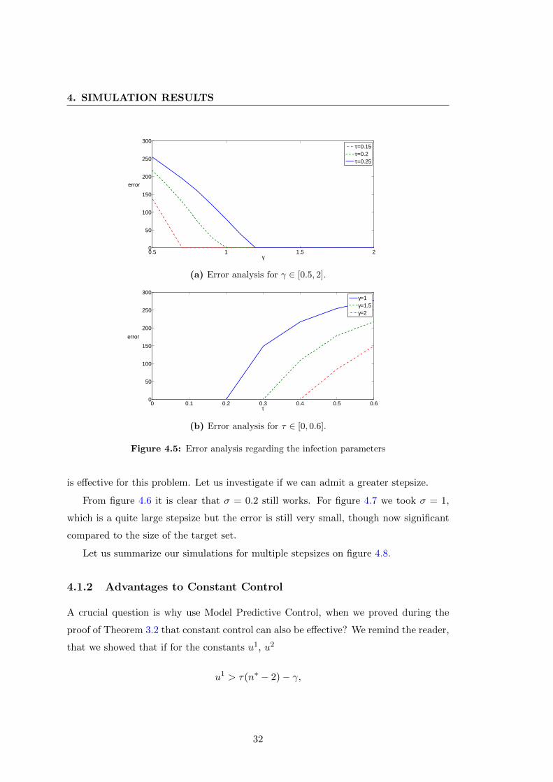
figure 4.5a we fixed a few values for τ , and the error is plotted with respect to γ. On

figure 4.5b γ is fixed, and we test a range of values for τ .

Let as move on to study the control stepsize σ. For this analysis we fix τ = 0.2 and

γ = 1 for the infection parameters. We have seen on figure 4.1 that a stepsize of σ = 0.1

31


0.5 1 1.5 20

50

100

150

200

250

300

γ

error

τ=0.15τ=0.2τ=0.25

(a) Error analysis for γ ∈ [0.5, 2].

0 0.1 0.2 0.3 0.4 0.5 0.60

50

100

150

200

250

300

τ

error

γ=1γ=1.5γ=2

(b) Error analysis for τ ∈ [0, 0.6].

Figure 4.5: Error analysis regarding the infection parameters

is effective for this problem. Let us investigate if we can admit a greater stepsize.

From figure 4.6 it is clear that σ = 0.2 still works. For figure 4.7 we took σ = 1,

which is a quite large stepsize but the error is still very small, though now significant

compared to the size of the target set.

Let us summarize our simulations for multiple stepsizes on figure 4.8.

4.1.2 Advantages to Constant Control

A crucial question is why use Model Predictive Control, when we proved during the

proof of Theorem 3.2 that constant control can also be effective? We remind the reader,

that we showed that if for the constants u1, u2

u1 > τ(n∗ − 2)− γ,

32

4.1 Results

0 5 10 150

2

4


t

[I]

0 5 10 150

1

2

3

4

5

t

u1

0 5 10 154.5

5

5.5

6Mean Degree

t

n

0 5 10 15−2

−1

0

1

2

3x 10

−3

t

u2

Figure 4.6: σ = 0.2, error = 0.

0 5 10 150

1

2

3

4


t

[I]

0 5 10 150

0.5

1

1.5

t

u1

0 5 10 155

5.2

5.4

5.6

5.8

6Mean Degree

t

n

0 5 10 15−2

0

2

4

6

8x 10

−3

t

u2

Figure 4.7: σ = 1, error = 9.6354 · 10−6.

and

u2 > 0

then Ed is an asymptotically stable fixed point of the system with constant controls

u1, u2: trajectories converge with an exponential speed from initial points sufficiently

close, so they also converge to the target set (since Ed ∈ Hε). Let us fix parameters

33


0.1 0.2 0.3 0.4 0.5 0.6 0.7 0.8 0.9 1 1.10

0.2

0.4

0.6

0.8

1

1.2x 10

−4

σ

error

τ=0.18τ=0.2τ=0.21

Figure 4.8: Error analysis regarding the stepsize for various infection rates.

similary to the Model Predictive Control’s investigation: N = 50, n(0) = 6, n∗ = 5,

I(0) = 5, [SI](0), [II](0) and [SS](0) as in (4.1a)–(4.1c), γ = 1 and τ = 0.2. For

this system the above conditions simplify to u1 > 0 (since u1 by definition is always

nonnegative) and u2 > 0. So any nonnegative control suffices. However, with some

controls convergence is much slower than with the MPC algorithm. So if we chose

randomly a constant value for u1 and u2 the system might not reach the target set in

simulation time — it is wiser to use MPC (compare it to figure 4.1). See for example

the case depicted on figure 4.9.

0 5 10 150

1

2

3

4


t

[I]

0 5 10 150

20

40

60

80

100

t

u1

0 5 10 154

4.5

5

5.5

6Mean Degree

t

n

0 5 10 150

0.02

0.04

0.06

0.08

0.1

t

u2

Figure 4.9: u1 = 100, u2 = 0.1, error = 8.2649.

To summarize the case of constant control with these parameters, we plotted the

34

4.1 Results

10 20 30 40 500

0.1

0.2

0.3

0.4

0.5

u1

u2

2

4

6

8

10

Figure 4.10: τ = 0.2, γ = 1.

error on figure 4.10 for various values of u1 and u2. One can see that for low values of

u2, the error is quite significant.

The same holds when a lower infection rate, τ = 1.5 is considered (and all else is

unchanged).

0 5 10 150

1

2

3

4


t

[I]

0 5 10 150

0.2

0.4

0.6

0.8

t

u1

0 5 10 155

5.2

5.4

5.6

5.8

6Mean Degree

t

n

0 5 10 150

0.002

0.004

0.006

0.008

0.01

t

u2

Figure 4.11: u1 = 0.6, u2 = 0.01, error = 2.8633.

Our numerous simulations show that in this case the MPC is algorithm is ’foolproof’

and the convergence is very fast (see figure 4.2).

35


But for the constant control, we are still able to choose ’weak’ parameters, such

that the convergence is slow (the trajectory does not reach the target set in simulation

time), see figure 4.11. We plotted a similar error analysis to the case of τ = 0.2 on

figure 4.12.

0 0.1 0.2 0.3 0.4 0.50

0.05

0.1

0.15

0.2

0.25

u1

u2

5

10

15

20

25

30

35

40

45

Figure 4.12: τ = 0.15, γ = 1.

4.1.3 An Alternative Cost Functional

We mentioned an alternative cost functional in section 2.4 of Chapter 2, namely

Jp(x0,u) =

p−1∑i=0

µ0‖xui ‖Hε + µ1∆u1i + µ2∆u2

i .

If µ1 and µ2 are chosen to be large compared to µ0, then the control computed

does not have large jumps in its value from step to step, since this is penalized in the

cost functional. This is to our benefit, since large jumps mean the deletion of many

connections in a short period of time, which is difficult in a real-world situation. But in

this case, reaching the target set will be of less priority, so the error will be larger. Let

us study the behaviour of the control and the controlled system for different choices of

µ0, µ1 and µ2. For all following simulations let the stepsize of the control be σ = 0.1,

and let us use the infection parameters τ = 0.2 and γ = 1.

Let us choose µ0 = 10−3 and first µ1 = µ2 = 10−3. One can see on figure 4.13 that

the jumps of the control are slight, compare it to figure 4.1 which was computed with

36

4.1 Results

the same parameters (except with our original cost functional). If we defined the ’size’

of the control as

s = maxt∈[0,15]

|u1(t)|+ maxt∈[0,15]

|u2(t)|,

then we could say that the size of the control in this case is considerably less, than in

the case depicted on figure 4.1.

0 5 10 151

2

3

4

5


t

[I]

0 5 10 150

1

2

3

4x 10

−3

t

u1

0 5 10 155.5

5.6

5.7

5.8

5.9

6Mean Degree

t

n

0 5 10 15−0.01

0

0.01

0.02

0.03

t

u2

Figure 4.13: µ0 = 10−3, µ1 = µ2 = 10−3, error = 13.8505.

0 5 10 150

2

4


t

[I]

0 5 10 150

0.01

0.02

0.03

t

u1

0 5 10 155

5.2

5.4

5.6

5.8

6Mean Degree

t

n

0 5 10 15−0.01

0

0.01

0.02

0.03

t

u2

Figure 4.14: µ0 = 10−3, µ1 = µ2 = 10−2, error = 4.0495.

37


This is because if the control functions cannot make large jumps in one step, they

cannot rise to a great absolute value on a finite time interval.

But the disadvantage of this control is that the convergence to the target set is

much slower, thus the error is considerable. Let us raise µ1 = µ2 to 10−2, the result

can be seen on figure 4.14. Now maxt∈[0,15]

|u1(t)| is larger, the control is more effective,

the error is less.

The summary of many tests can be seen on figure 4.15. The error of the dark red

area is the error of the zero control (u1 ≡ 0, u2 ≡ 0): for such choice of the parameters

µ0, µ1, µ2 the jumps of the control are penalized so heavily, that the control functions

cannot change their initial zero state, so zero control is applied. This is of course not

for our advantage, we should choose values for µ0, µ1, µ2 such that the error is low,

pictured dark blue on our figure.

0 2 4 6 8−8

−7

−6

−5

−4

−3

−2

−1

0

µ1=µ

2

µ0

5

10

15

20

25

30

35

40

45

Figure 4.15: Error analysis regarding the parameters of the cost functional on a base 10

log log scale.

38

5

Discussion

In this thesis we investigated a mathemathical model of a general epidemic and the

question of controlling the disease. Our network-based SIS epidemic model was con-

trolled with the means of structural intervention: we deleted and created connections

keeping two objectives in mind, remove infection from the population while maintaining

social cohesion.

The formulated control differs from classic approaches, since it focuses on reaching

a favourable overall state of the population instead of minimizing the economical cost

of the intervention. However, it is an interesting possibility for further improvement in

our model to build in the monetary cost of the structural changes made in the social

network of the population.

We studied the stability properties of the control and came to the conclusion that

the stability can be proved when the intitial state of the system is sufficiently close to

the target set. There is much improvement to be made, it would be very useful to prove

stability formally for a wider subset of all possible initial states. Our simulations allow

us to believe this might be true, proving this is an intriguing task for further research.

We examined our model for various choices of infection and control parameters with

simulations. We learned that the convergence to the target set is much slower if the

infection rate is high compared to the recovery rate. To improve this, it would be

effective to combine our algorithm of structural changes with medical intervention, for

example vaccination or medication. We also learned that our algorithm has a very nice

numerical property, it admits a relatively large stepsize.

39

5. DISCUSSION

For further research, it would be interesting to study concrete networks, and how

our method could be improved if more information of the network structure could be

built in the representing SIS model.

40

Appendix A

Matlab Software

1 function [] = nmpc(step)

2 %NMPC: Nonlinear Model Predictive Control

3 %Input: step - stepsize of the control algorithm

4 %Output: plot

5

6

7 %Set parameters

8 N = 50;

9 Tmax = 151;

10

11 p = 1;

12 tau = 0.2;

13 n = 6;

14 i = 5;

15

16 M1=1000;

17 M2=1000;

18

19 %Initialization

20 y = initial value(N,n,i);

21

22 u1 = zeros(p,1);

23 u2 = zeros(p,1);

24

25 %Main part

26 for t = 1:Tmax

27

28 control1(t) = u1(1);

41

A. MATLAB SOFTWARE

29 control2(t) = u2(1);

30

31 output1(t) = y(1);

32 output2(t) = (2*y(2) + y(3) + y(4))/N;

33

34 u 0 = [u1 u2];

35

36 control10 = control1(t);

37 control20 = control2(t);

38

39 u = lsqnonlin(@optimization,u 0,[0 -M2],[M1 M2],[],y,step,control10,...

40 control20,tau);

41

42 u1 = u(1:p);

43 u2 = u(p+1:2*p);

44

45 y new = msis solver(u1(1),u2(1),y,step,tau);

46 y = y new;

47

48 end

49

50 %Plot results

51

52 T1 = step*(0:1:Tmax-1);

53

54 grey = [0.5 0.5 0.5];

55

56 subplot(2,2,1), plot(T1,output1(1:Tmax),'-r','LineWidth',2)

57 title('Infected Population')

58 xlabel('t')

59 ylabel('[I]')

60 set(get(gca,'ylabel'),'Rotation',0.0)

61 xlim([0 15])

62 hold off

63

64 subplot(2,2,2),

65 for i=1:Tmax-1

66 plot([(i-1)*step,i*step],[control1(i) control1(i)],'Color',grey,...

67 'LineWidth',2)

68 hold on

69 end

70 hold off

71 xlabel('t')

72 ylabel('uˆ1')


42

74 xlim([0 15])

75

76 subplot(2,2,3), plot(T1,output2(1:Tmax),'-r','LineWidth',2)

77 title('Mean Degree')

78 xlabel('t')

79 ylabel('n')


81 xlim([0 15])

82 hold off

83

84 subplot(2,2,4),

85 for i=1:Tmax-1

86 plot([(i-1)*step,i*step],[control2(i) control2(i)],'Color',grey,...

87 'LineWidth',2)

88 hold on

89 end

90 hold off

91 xlabel('t')

92 ylabel('uˆ2')


94 xlim([0 15])

95

96 end

1 function y = initial value(Np,n,I)

2 %INITIAL VALUE: Compute initial value

3 %Input: Np - size of population

4 % n - initial mean degree

5 % i - number of initially infected

6 %Output: y - vector of initial values for I, IS, II and SS

7

8

9 IS = n*I*(Np-I)/(Np-1);

10 II = n*I*(I-1)/(Np-1);

11 SS = n*(Np-I)*(Np-I-1)/(Np-1);

12

13 y = [I IS II SS];

14

15 end

1 function L = optimization(u,y,step,control10,control20,tau)

43

A. MATLAB SOFTWARE

2 %OPTIMIZATION: construct cost functional

3 %Input to lsqnonlin

4 %Input parameters: step - stepsize of control

5 % tau - infection rate

6

7

8 %Set parameters

9 p=1;

10 mu0=1;

11 mu1=20;

12 mu2=20;

13

14 %Calculate predictions for future output

15 y new(:,1) = msis solver(u(1),u(p+1),y,step,tau);

16

17 for j=2:p,

18 y new(:,j) = msis solver(u(j),u(j+p),y new(:,j-1),step,tau);

19 end

20

21 delta u1(1) = u(1) - control10;

22

23 %Calculate jumps of the control

24 for j=2:p,

25 delta u1(j) = u(j) - u(j-1);

26 end

27

28 delta u2(1) = u(p+1) - control20;

29

30 for j=2:p,

31 delta u2(j) = u(j+p) - u(j+p-1);

32 end

33

34 %Calculate distance of predictions from the target set

35 y dist = sqrt(y new(1,1)ˆ2+y new(2,1)ˆ2+y new(3,1)ˆ2+ ...

36 (y new(4,1)-N*5)ˆ2) - eps;

37

38 %Cost functional

39 L = [sqrt(mu0)*y dist sqrt(mu1)*delta u1 sqrt(mu2)*delta u2];

40

41

42 end

1 function [y new] = msis solver(u1,u2,y,step,tau)

44

2 %MSIS SOLVER: solve system on interval [0 step]

3 %Input: u1 - control 1

4 % u2 - control 2

5 % y - initial value

6 % step - control stepsize


8

9 N = 50;

10

11 [T,Y] = ode45(@msis eq,[0 step], y, [], u1, u2, N, tau);

12

13 I = Y(:,1);

14 r1 = length(I);

15

16 IS = Y(:,2);

17 r2 = length(IS);

18

19 II = Y(:,3);

20 r3 = length(II);

21

22 SS = Y(:,4);

23 r4 = length(SS);

24

25 y new=[I(r1); IS(r2); II(r3); SS(r4)];

1 function dy = msis eq(t,y,u1,u2,N,tau)

2 %SIS EQ: the equation

3 %Input: u1 - control 1

4 % u2 - control 2

5 % N - size of population


7 %

8 %y(1) = I

9 %y(2) = SI

10 %y(3) = II

11 %y(4) = SS

12

13 gamma = 1;

14

15 dy = zeros(4,1);

16

17 dy(1) = tau*y(2) - gamma*y(1);

18

45

A. MATLAB SOFTWARE

19 dy(2) = gamma*(y(3) - y(2)) + tau*(((((2*y(2)+y(3)+y(4))/N) - 1)/...

20 ((2*y(2)+ y(3)+y(4))/N))*((y(4)*y(2))/(N - y(1))) - ((((2*y(2)+y(3)...

21 +y(4))/N) - 1)/((2*y(2)+ y(3)+y(4))/N))*((y(2)*y(2))/(N - y(1))) - ...

22 y(2)) - u1*y(2);

23

24 dy(3) = -2*gamma*y(3) + 2*tau*(((((2*y(2)+y(3)+y(4))/N) - 1)/((2*y(2)...

25 +y(3)+y(4))/N))*((y(2)*y(2))/(N - y(1))) + y(2));

26

27 dy(4) = 2*gamma*y(2) - 2*tau*(((((2*y(2)+y(3)+y(4))/N) - 1)/((2*y(2)...

28 +y(3)+y(4))/N))*((y(4)*y(2))/(N - y(1)))) + max(u2,0)*((N - y(1))*...

29 (5 - y(1))- y(4)) + min(u2,0)*y(4);

46

Bibliography

[1] Roy M. Anderson and Robert M. May. Infectious diseases of humans: dynamics

and control, volume 28. Wiley Online Library, 1992. 1, 3

[2] Eduardo F. Camacho and Carlos Bordons Alba. Model Predictive Control.

Springer, 2013. 8, 10

[3] Charles R. Cutler and Brian C. Ramaker. Dynamic Matrix Control- a computer

control algorithm. Automatic Control Conference, San Francisco, 1980. 8

[4] Odo Diekmann and JAP Heesterbeek. Mathematical epidemiology of infectious

diseases, volume 14. Wiley Chichester, 2000. 3

[5] John R. Dormand and Peter J. Prince. A family of embedded Runge–Kutta for-

mulae. J. Comput. Appl. Math., 6(1):19–26, 1980. 26, 28

[6] Sever Silvestru Dragomir. Some Gronwall type inequalities and applications.

RGMIA Monographs. Victoria University, 2000. 19

[7] Lars Grune. Analysis and design of unconstrained nonlinear MPC schemes for

finite and infinite dimensional systems. SIAM J. Control Optim., 48(2):1206–1228,

2007. 15, 17

[8] Lars Grune and Jurgen Pannek. Nonlinear Model Predictive Control. Springer,

2011. 17, 21

[9] Eva Gyurkovics. Sampled-data control and stability of sets for nonlinear systems.

Differential Equations and Dynamical Systems, 17(1-2):169–183, 2009. 22, 24

[10] Matt Keeling. The implications of network structure for epidemic dynamics. Theor.

Popul. Biol., 67(1):1–8, 2005. 5

47

BIBLIOGRAPHY

[11] Matt J. Keeling and Pejman Rohani. Modeling infectious diseases in humans and

animals. Princeton University Press, 2008. 3

[12] William O. Kermack and Anderson G. McKendrick. A contribution to the math-

ematical study of epidemics. Proc. R. Soc. London Ser, 115:700–721, 1927. 3

[13] Istvan Z. Kiss, Darren M. Green, and Rowland R. Kao. Disease contact tracing in

random and clustered networks. P. Roy. Soc. B-Biol. Sci., 272(1570):1407–1414,

2005. 1

[14] Fanni Selley, Adam Besenyei, Istvan Z. Kiss, and Peter L. Simon. Dynamic control

of modern, network-based epidemic models. arXiv preprint arXiv:1402.2194, 2014.

[15] Peter L. Simon. Bifurkaciok komplex rendszerek differencialegyenleteiben.

Akademiai doktori ertekezes, 2012. 5, 6

[16] Minus Van Baalen. Pair approximations for different spatial geometries, In: Dieck-

mann, U., law, R., metz, J. A. J. (eds.). The geometry of ecological interactions:

simplifying spatial complexity, pages 359–387. 5

48

Documents

Receding Horizon Control of an SIS Epidemic: Optimality and Asymptotic ...web.cs.elte.hu/blobs/diplomamunkak/msc_mat/2014/selley_fanni.pdf · an SIS Epidemic: Optimality and Asymptotic