Clemson UniversityTigerPrints

All Theses Theses

8-2007

NONLINEAR MODELING OF THEADSORPTION-INDUCED SURFACE STRESSIN PIEZOELECTRICALLY-DRIVENMICROCANTILEVER BIOSENSORSMana AfshariClemson University, mafshar@clemson.edu

Follow this and additional works at: https://tigerprints.clemson.edu/all_theses

Part of the Engineering Mechanics Commons

This Thesis is brought to you for free and open access by the Theses at TigerPrints. It has been accepted for inclusion in All Theses by an authorizedadministrator of TigerPrints. For more information, please contact kokeefe@clemson.edu.

Recommended CitationAfshari, Mana, "NONLINEAR MODELING OF THE ADSORPTION-INDUCED SURFACE STRESS INPIEZOELECTRICALLY-DRIVEN MICROCANTILEVER BIOSENSORS" (2007). All Theses. 154.https://tigerprints.clemson.edu/all_theses/154

NONLINEAR MODELING OF THE ADSORPTION-INDUCED SURFACE STRESS IN PIEZOELECTRICALLY-DRIVEN MICROCANTILEVER

BIOSENSORS _____________________________________

A Thesis Presented to

the Graduate School of Clemson University

_____________________________________

In Partial Fulfillment of the Requirements for the Degree

Master of Science Mechanical Engineering

_____________________________________

by Mana Afshari August 2007

_____________________________________

Accepted by: Nader Jalili, Committee Chair

Darren M. Dawson Mohammed F. Daqaq

ABSTRACT

Microcantilever-based biosensors are rapidly becoming an enabling

sensing technology for a variety of label-free biological applications due to their

extreme applicability, versatility and low cost. These sensors operate through the

adsorption of species on the functionalized surface of microcantilevers. The

adsorption of biological species induces surface stress which originates from the

molecular interactions such as adhesion forces of attraction/repulsion,

electrostatic forces or the surface charge redistribution of the underlying substrate.

This surface stress, consequently, alters the resonance frequency of the

microcantilever beam.

This study presents a general framework towards modeling resonance

frequency changes induced due to the surface stress arising from the adsorption of

biological species on the surface of the microcantilever. Very few works have

dealt with the effect of surface stress on the resonance frequency shifts of

microcantilevers and mainly assume a simple model for the vibrating

microcantilever beam. In the proposed modeling framework, the nonlinear terms

due to beam's flexural rigidity from macro- to micro-scale as well as varying

nature of the adsorption induced surface stress are considered.

iv

It is first shown that the nonlinearity of the system originates from two

different sources; namely, microcantilever flexural rigidity and adsorption

induced surface stress. All these nonlinearities are formulated into the general

equation of motion of the vibrating microcantilever. It is then shown that the

dynamic mode of biosensing formulated in the paper is much more sensitive than

the static mode to the change in the properties of the adsorbed biological species.

DEDICATION

To my family in Iran and my friends in Clemson

vi

ACKNOWLEDGMENTS

I sincerely thank my advisor, Dr. Nader Jalili for his support and guidance

during my Master's studies in every aspect. It was a great chance to work in his

research group, which left me with many wonderful qualities. Helpful suggestions

from my advisory committee members, Dr. Darren M. Dawson and Dr.

Mohammed F. Daqaq, and the financial supports through National Science

Foundation under CAREER Grant No. DMI-0238987, are also greatly

appreciated.

viii

TABLE OF CONTENTS

Page

TITLE PAGE............................................................................................... i

ABSTRACT................................................................................................. iii

DEDICATION............................................................................................. v

ACKNOWLEDGEMENTS......................................................................... vii

LIST OF TABLES....................................................................................... xiii

LIST OF FIGURES ..................................................................................... xv

CHAPTER

1. INTRODUCTION ......................................................................... 1

Research Motivation .............................................................. 1

Thesis Overview .................................................................... 2

2. MICROCANTILEVER-BASED SENSING................................. 5

Background and Literature Review ....................................... 6

Microcantilever-based Sensing Applications ........................ 7

Surface Stress Sensing ................................................. 8

Ultra-small Mass Sensing ............................................ 12

Temperature Sensing ................................................... 12

3. MICROCANTILEVER-BASED BIOSENSING .......................... 13

Different Methods of Biosensing........................................... 14

Quartz Crystal Microbalance (QCM) .......................... 14

Microcantilever Biosensors’ Modes of Detection ................. 17

Static Mode .................................................................. 17

Uniform Curvature Assumption and Modeling

the Surface Stress................................................... 20

Static Deflection based on Energy Dissipation............ 23

x

Table of Contents (Continued)

Page

Static Deflection based on the Molecular

Interactions............................................................. 24

Dynamic Mode............................................................. 27

Taut-String Model Approximation .............................. 27

Beam with Axial Force Model Approximation ........... 28

Utilizing Buckling Analogy in Formulating the

Adsorption-induced Shift in Resonance

Frequency............................................................... 30

Recent Developments of the Microcantilever

Biosensors .............................................................................. 31

Sensitivity Enhancement.............................................. 31

Potential and Practical Medical Applications .............. 35

4. NONLINEAR MODELING OF PIEZOELECTRICALLY-

DRIVEN MICROCANTILEVER BIOSENSORS.................. 39

Piezoelectric Actuators .......................................................... 40

Molecular Arrangement of the Adsorbed Biological

Species and the Modeling the Adsorption Induced

Surface Stress................................................................... 43

Origin of the Adsorption Induced Surface Stress .................. 44

Intermolecular Forces of Attraction and Repulsion............... 45

Lennard-Jones Constants of A and B ..................................... 47

Electrostatic Forces................................................................ 50

Capillary Forces ..................................................................... 51

The General Equation of Motion

Microcantilever utilizing Hamilton’s Principle ............... 52

Potential Energy of the Microcantilever Beam...................... 54

Potential Energy due to the Beam’s Structure Having

the PZT Layer on Its Surface ........................................... 54

Potential Energy due to the energy storage of PZT Layer..... 56

Potential Energy due to the Adsorbed Biological Layer ....... 58

Total Potential Energy of the Microcantilever Beam

with the PZT Layer and the Adsorbed Biological

Layer ................................................................................ 60

Kinetic Energy of the Microcantilever Beam ........................ 60

General Equation of Motion of the Microcantilever

Beam ................................................................................ 61

xi

Table of Contents (Continued)

Page

5. SOLUTION TO THE NONLINEAR EQUATIONS OF

MOTION.................................................................................. 71

Numerical Simulations and Results ....................................... 73 The Effect of the Attached PZT Layer .................................. 78

The Effect of Both PZT and the Adsorbed Biological

Layers............................................................................... 80

6. SENSITIVITY STUDY OF THE STATIC MODE

DETECTION ........................................................................... 83

A New Approach toward Solution of the Nonlinear

Equation of Motion .......................................................... 84

Numerical Simulations and Results ....................................... 87

Sensitivity of the Static vs. the Dynamic Detection

Mode ................................................................................ 89

7. CONCLUSIONS AND FUTURE WORK.................................... 93

Conclusions............................................................................ 93

Future Work and Directions................................................... 94

APPENDIX: SAMPLE CODES AND BLOCK DIAGRAMS

USED FOR NUMERICAL SIMULATIONS AND

EXPERIMENTS.............................................................................. 97

REFERENCES ...................................................................................... 103

xii

LIST OF TABLES

Table Page

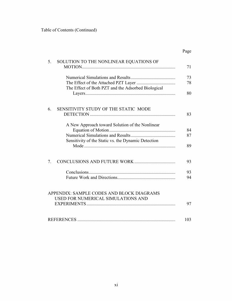
4.1 Lattice structure for some elements ................................................... 49

5.1 Experimental resonance frequencies before (f1), and after

adsorption (fads), and the variation in microcantilever’s

resonance frequency (∆) .............................................................. 75

5.2 Simulation results for constants A and B and the corresponding

frequency...................................................................................... 76

5.3 Simulation results for constants A and B and the corresponding

frequencies for PZT-driven microcantilever................................ 81

xiv

LIST OF FIGURES

Figure Page

2.1 Schematic behaviour of the adsorbed biological species on the

surface of a microcantilever and their molecular interactions ..... 5

2.2 Schematic of the DNA hybridization experiment. Each

cantilever is functionalized on one side with a different

oligonucleotide base sequence, (a) before the injection and

adsorption of the biological species, (b) after the injection

of the first complementary oligonucleotide, where the

hybridization occurs on the cantilever and deflects

it for an amount of ∆x .................................................................. 8

2.3 Schematic of a microcantilever biosensor, (a) having only

one functionalized surface and studied via the static detection

mode, (b) having both surfaces functionalized hence studied

via the dynamic detection mode .................................................. 9

2.4 Schematic of the absorption-induced surface stress sensing ............. 10

2.5 Schematic of the spontaneous adsorption of straight-chain

thiol molecules on a gold coated cantilever ................................. 11

3.1 Schematic of a cantilever chemical sensor with optical lever

readout. Microcantilever surfaces modified with (a) nanobeads,

(b) cavitand receptors, and (c) thin polymeric film to improve

cantilever response or selectivity. (d) Depiction of a

bioaffinity interaction microcantilever ........................................ 13

3.2 Schematic of the quarts crystal which is the main part of a QCM .... 15

3.3 Schematic of a commercially available quartz crystal

microbalance ................................................................................ 16

3.4 Schematic diagram showing loading of free edges of cantilever

plate by moments per unit length / 2appM t= ∆σ ....................... 22

xvi

List of Figures (Continued)

Figure Page

3.5 Schematic of the uniformly distributed surface stress model ............ 23

3.6 Arrangement of atoms (or molecules) on cantilever surface ............. 25

3.7 Position of surface atoms (or molecules) on the deflected

microcantilever beam................................................................... 26

3.8 Taut-string approximation of the microcantilever beam ................... 28

3.9 Schematic view of a microcantilever with uniform surface

stress............................................................................................. 29

3.10 Microcantilever with fractional surface stresses coverage ................ 29

3.11 Scheme of microcantilever based DNA detection ............................. 35

3.12 Surface of a microcantilever biosensor covered with E. coli............. 36

3.13 Schematic of mass increase due to bacterial growth on the

surface of microcantilever sensor: (a) Freshly adsorbed

E. coli cells on the surface of microcantilever, (b) The

bacterial cells start to grow .......................................................... 36

3.14 SEM image of Listeria innocua bacteria nonspecifically

adsorbed on the surface of a microcantilever .............................. 37

3.15 A microcantilever beam utilized for the mass sensing of the

adsorbed vaccinia virus particle................................................... 38

4.1 Schematic of a microcantilever biosensor with the attached

biological species and the piezoelectric layer on its surface........ 40

4.2 (a) A stacked design piezoelectric actuator, (b) A laminar

design piezoelectric actuator........................................................ 42

4.3 PZT strip bonded to the surface of a beam ........................................ 43

xvii

List of Figures (Continued)

Figure Page

4.4 Arrangement of a monolayer of the adsorbed biological

species on microcantilever surface before the deflection of

the microcantilever beam............................................................. 44

4.5 Schematic of a fully assembled alkane thiol SAM............................ 44

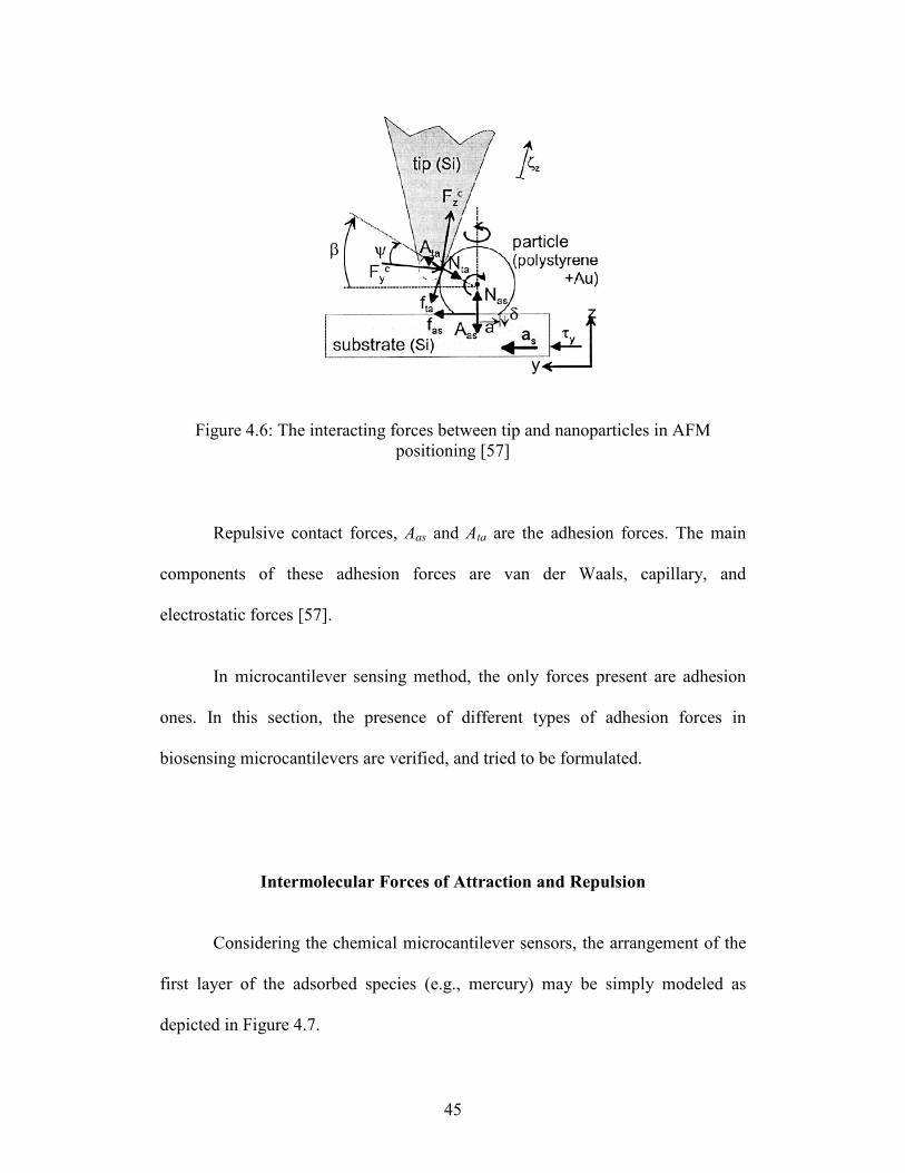
4.6 The interacting forces between tip and nanoparticles in AFM

positioning.................................................................................... 45

4.7 Arrangement of the adsorbed atoms (molecules) on

microcantilever surface................................................................ 46

4.8 (a) Steady-state cantilever deflections caused by

immobilization of ssDNA (sequence K-30) at different PB

concentrations, (b) Steady-state changes in cantilever

deflection for hybridization of 30-nt-long ssDNA

(sequences K-30 and K9-30) at different PB

concentrations .............................................................................. 51

4.9 Schematic of capillary effect during a sphere and flat surface

contact, with e being the initial thickness of the water, h the

tip-surface distance, r and ρ the radii of curvature of the

meniscus....................................................................................... 52

4.10 (a) Schematic of the microcantilever with the PZT and the

adsorbed biological layers on its surface, (b) Coordinate

system of the microcantilever beam ............................................ 53

4.11 Schematic of a segment of the microcantilever beam and the

PZT layer on its surface ............................................................... 55

4.12 Arrangement of a monolayer of biological species on

microcantilever surface after the deflection of microcantilever .. 59

5.1 Frequency response of a microcantilever with properties listed

in Eq. (5.12) and the adsorbed biological species on its

surface having Lennard-Jones constants of

A=1.3×10-72 J.m6 and B=0.4×10-135 J.m12

.................................... 77

xviii

List of Figures (Continued)

Figure Page

5.2 Linear frequency response of the PZT-driven microcantilever ......... 79

5.3 Nonlinear frequency response of the PZT-driven

microcantilever ............................................................................ 80

5.4 Nonlinear frequency response of the PZT-driven

microcantilever covered by a biological layer with

A=1×10-72 J.m6 and B=0.4×10-135 J.m12

....................................... 82

6.1 The static deflection of the microcantilever with

length=500 (µm), width= 100 (µm) and thickness=1 (µm) ......... 88

6.2 The static deflection of five microcantilever beams differing

only in their lengths ..................................................................... 89

6.3 Different static deflections of the PZT-driven microcantilever

with the properties listed in Eqs. (6.13) and (6.14) for

different Lennard-Jones A constants............................................ 90

6.4 Resonance frequencies of the first mode of vibration for the

PZT-driven microcantilever with the properties listed in

Eqs. (6.13) and (6.14) for different Lennard-Jones A

constants....................................................................................... 91

7.1 Cantisense functionalisation unit ....................................................... 95

7.2 Polytec state-of-the-art micro system analyzer MSA 400 ................. 96

A.1 Simulink® block diagram of deriving the frequency

response of the vibrating microcantilever beam .......................... 97

CHAPTER 1

INTRODUCTION

Research Motivation

Microcantilever-based biosensors are rapidly becoming an enabling

sensing technology for a variety of label-free biological applications due to their

extreme applicability, versatility and low cost. These sensors operate through the

adsorption of species on the functionalized surface of microcantilevers.

Very few works have dealt with modeling the effect of surface stress on

the resonance frequency shifts of microcantilevers and mainly assume a simple

model for the vibrating microcantilever beam. Studying “macro-scale” cantilever

beams, these simple models provide relatively good representation of the physical

systems. For the case of microcantilevers, however, the molecular forces are no

longer negligible and must be taken into account in modeling the surface stress.

Thesis Overview

This thesis presents a general framework towards modeling resonance

frequency changes induced due to the surface stress arising from the adsorption of

biological species on the surface of the piezoelectrically-driven microcantilever.

2

The molecular interactions of the adsorbed biological species which

induce the surface stress are explained in Chapter 4 and the attraction/repulsion

forces are considered in the potential energy formulation.

Utilizing the Hamilton’s principle, the general equation of motion of the

resonating microcantilever is also formulated in Chapter 4. In the proposed

modeling framework derived in Chapter 4, the nonlinear terms due to beam’s

flexural rigidity from macro- to micro-scale as well as varying nature of the

adsorption induced surface stress are considered. It is first shown that the

nonlinearity of the system originates from two different sources; namely,

microcantilever flexural rigidity and adsorption induced surface stress.

Through numerical simulation given in Chapter 5, it is demonstrated that

the nonlinearity due to the surface stress does not have a considerable effect on

the resonance frequency change of the microcantilever. However, nonlinearity

due to flexural rigidity (which is directly attributed to beam’s dimensions) plays

an important role in the resonance frequency shift, and hence, in the resultant

molecular recognition capability.

A new method of formulating the adsorption induced surface stress as a

function of the static deflection of the microcantilever is given in Chapter 6. Most

of the previous works in this area are based on the Stoney’s simple equation. In

the proposed method, the molecular interactions of the adsorbed biological

species are modeled based on the Lennard-Jones attraction/repulsion potential.

As a result, the sensitivity of the static detection mode (based on the proposed

3

method) is compared to that of the dynamic mode. It is shown that the dynamic

mode of biosensing is much more sensitive to the change in the properties of the

adsorbed biological species, when compared to conventional static mode

detection mechanism.

4

CHAPTER 2

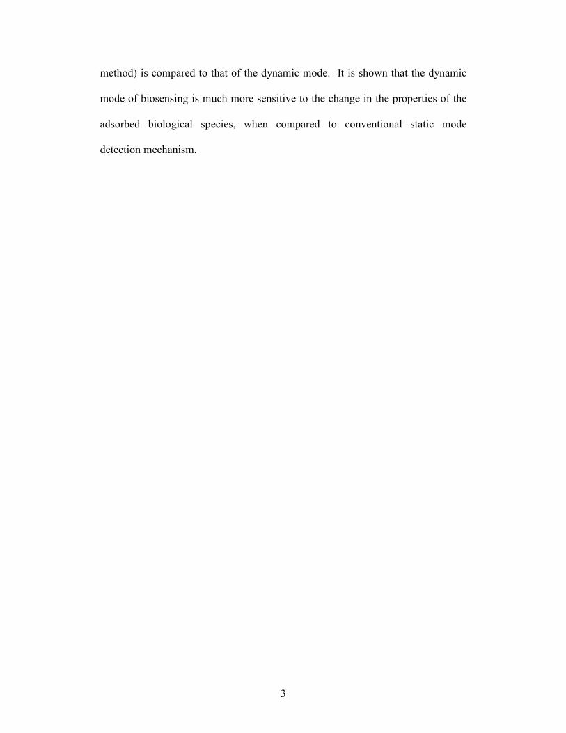
MICROCANTILEVER-BASED SENSING

Recently, microfabricated silicon cantilevers for atomic force microscopy

(AFM) have been used to measure changes in the surface stress of solids or the

added mass to their surface. These experiments lead to the idea of making

extremely sensitive sensor platform for chemical and biological detections, as

schematically depicted in Figure 2.1.

Figure 2.1: Schematic behaviour of the adsorbed biological species on the surface

of a microcantilever and their molecular interactions

6

Background and Literature Review

The idea of applying macroscopic cantilevers goes back to about a century

ago, when Stoney utilized cantilevers’ deflection for measuring the deposition

induced surface stress of beams in an electrochemical environment [59] and

Galileo performed cantilevers as platforms for investigating the strength of

materials [44]. In late 70’s, Taylor et al. utilized cantilevered beam sensors for the

detection of gasses [62].

Microcantilevers were first used in Scanning Force Microscopy (SFM).

These microcantilevers deflect due to the interaction forces between their tip and

the sample. It was observed that temperature variations and adsorption of vapors

cause parasitic cantilever deflection in SFM [66]. Although this parasitic

deflection was undesirable for the SFM, it triggered the idea of applying

microcantilevers as chemical and temperature sensors. Thundat et al. showed that

the resonance frequency variation of SFM cantilevers can be used for measuring

the amount of loaded mass of the adsorbed water and mercury vapors [66].

Simultaneously, Gimzewski et al. used micromachined cantilevers as

temperature and heat flow sensors and as calorimeters for measuring the heat

generated by chemical reactions [4, 5, 22]. It is important to note that in 1993

(prior to Thundat et al. and Gimzewski et al.’s investigations) Cleveland et al.

utilized microcantilevers’ sensing potential for precisely calculating the spring

constant of the SFM microcantilevers. Their nondestructive method included the

addition of small masses at the end of the microcantilevers and measuring the

7

resulting shift in resonance frequency of the beam [14]. Although they established

a unique calibration method for SFM microcantilevers, they did not pay attention

to the unrevealed sensing potential of microcantilevers and missed the opportunity

of being the pioneers in the field of microcantilever sensing. Cleveland et al.’s

method was later modified due to its low accuracy resulting from the practical

difficulties and errors of placing the added mass at a specific position on the

microcantilevers [52].

From the observations of Thundat et al. in Oak Ridge National Laboratory

and Gimzewski et al. in IBM Zurich Research Laboratory and Cambridge

University, a new era was established in sensor technology. Microcantilever

sensors attracted a lot of attention due to their simplicity, extremely small size and

potential for extremely high sensitivity.

Microcantilever-based Sensing Applications

In the beginning, microcantilevers were mainly utilized as chemical [36,

49, 63, 65, 68], thermal [10, 13, 17, 36, 46, 48] and physical [44, 45, 69] sensors.

These sensors were generally considered to perform in air or in vacuum, resulting

in the ignorance of environmental damping effect on the resonance frequency of

microcantilevers. Utilizing microcantilever sensors for studying biological

systems under native conditions and investigating processes at liquid-solid

interface brought the idea of considering the damping effect of the surrounding

8

media on the resonance frequency of microcantilevers [70]. It was not until 1996,

when the applicability and potential of microcantilevers as biosensors attracted

attention [6, 7, 9].

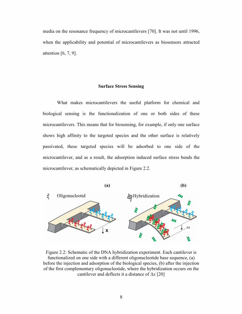
Surface Stress Sensing

What makes microcantilevers the useful platform for chemical and

biological sensing is the functionalization of one or both sides of these

microcantilevers. This means that for biosensing, for example, if only one surface

shows high affinity to the targeted species and the other surface is relatively

passivated, these targeted species will be adsorbed to one side of the

microcantilever, and as a result, the adsorption induced surface stress bends the

microcantilever, as schematically depicted in Figure 2.2.

Figure 2.2: Schematic of the DNA hybridization experiment. Each cantilever is

functionalized on one side with a different oligonucleotide base sequence, (a)

before the injection and adsorption of the biological species, (b) after the injection

of the first complementary oligonucleotide, where the hybridization occurs on the

cantilever and deflects it a distance of ∆x [20]

Oligonucleotid

e Hybridization

(a) (b)

9

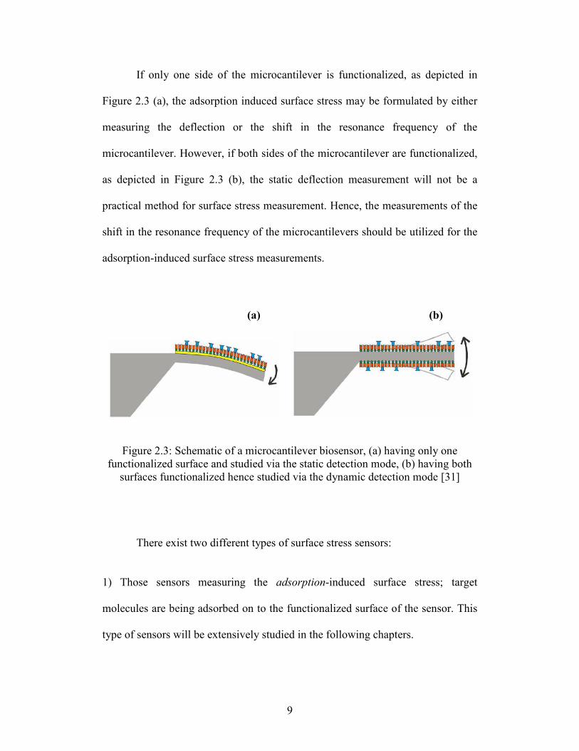
If only one side of the microcantilever is functionalized, as depicted in

Figure 2.3 (a), the adsorption induced surface stress may be formulated by either

measuring the deflection or the shift in the resonance frequency of the

microcantilever. However, if both sides of the microcantilever are functionalized,

as depicted in Figure 2.3 (b), the static deflection measurement will not be a

practical method for surface stress measurement. Hence, the measurements of the

shift in the resonance frequency of the microcantilevers should be utilized for the

adsorption-induced surface stress measurements.

Figure 2.3: Schematic of a microcantilever biosensor, (a) having only one

functionalized surface and studied via the static detection mode, (b) having both

surfaces functionalized hence studied via the dynamic detection mode [31]

There exist two different types of surface stress sensors:

1) Those sensors measuring the adsorption-induced surface stress; target

molecules are being adsorbed on to the functionalized surface of the sensor. This

type of sensors will be extensively studied in the following chapters.

(a) (b)

10

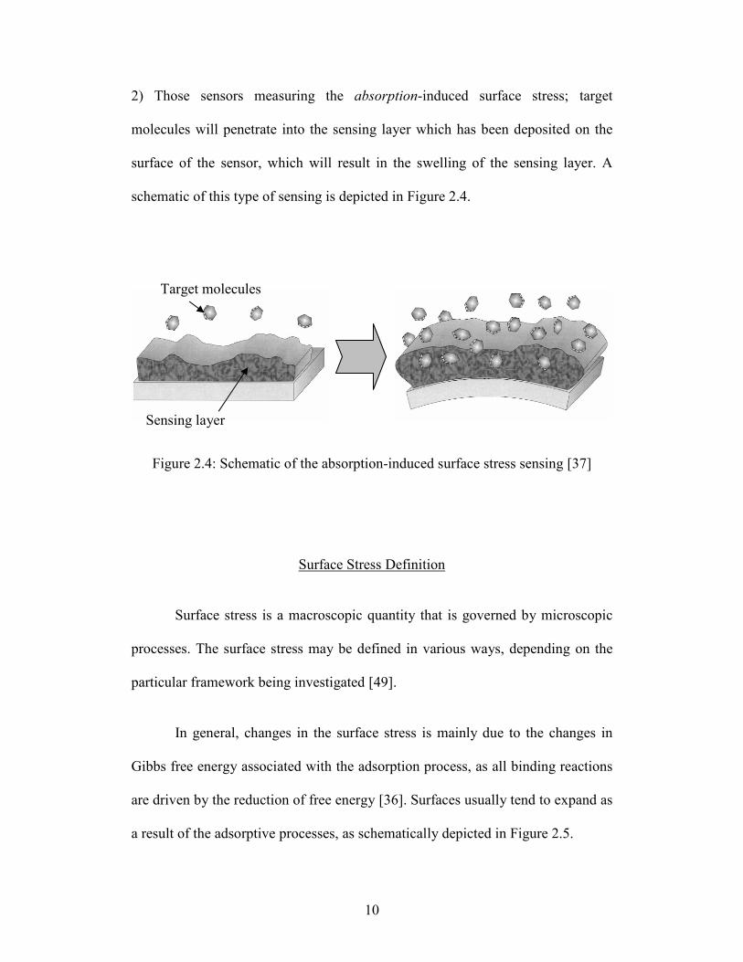
2) Those sensors measuring the absorption-induced surface stress; target

molecules will penetrate into the sensing layer which has been deposited on the

surface of the sensor, which will result in the swelling of the sensing layer. A

schematic of this type of sensing is depicted in Figure 2.4.

Figure 2.4: Schematic of the absorption-induced surface stress sensing [37]

Surface Stress Definition

Surface stress is a macroscopic quantity that is governed by microscopic

processes. The surface stress may be defined in various ways, depending on the

particular framework being investigated [49].

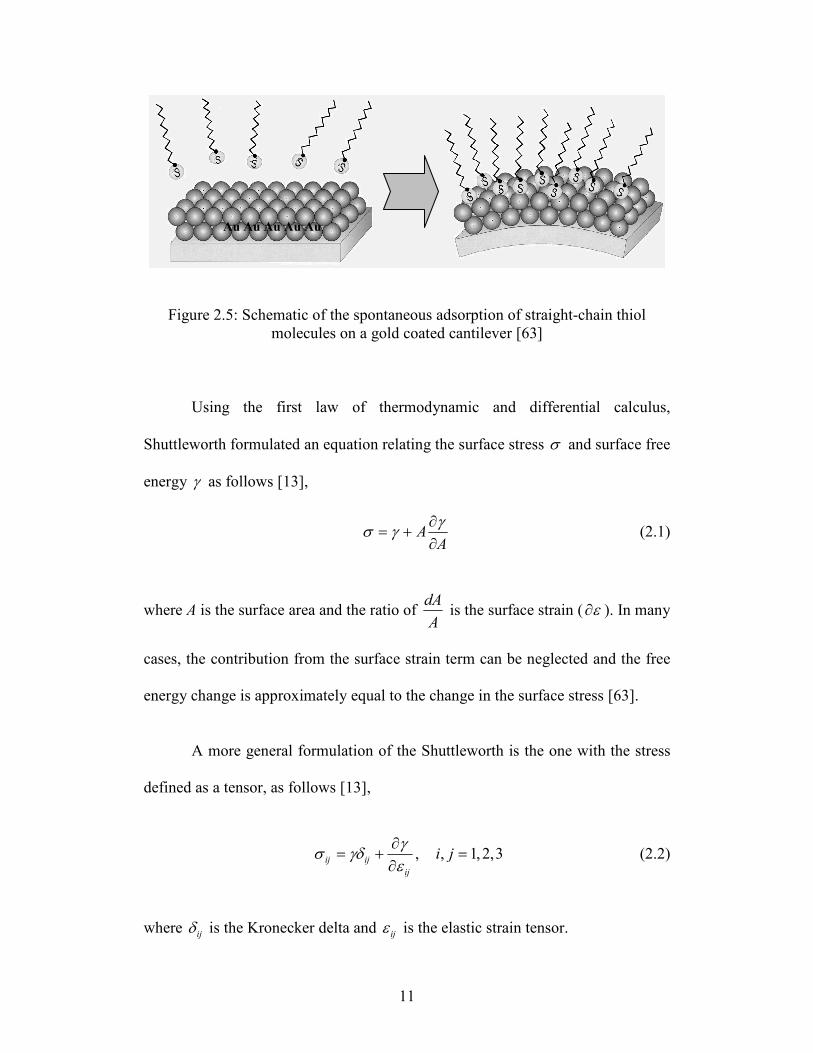
In general, changes in the surface stress is mainly due to the changes in

Gibbs free energy associated with the adsorption process, as all binding reactions

are driven by the reduction of free energy [36]. Surfaces usually tend to expand as

a result of the adsorptive processes, as schematically depicted in Figure 2.5.

Target molecules

Sensing layer

11

Figure 2.5: Schematic of the spontaneous adsorption of straight-chain thiol

molecules on a gold coated cantilever [63]

Using the first law of thermodynamic and differential calculus,

Shuttleworth formulated an equation relating the surface stress σ and surface free

energy γ as follows [13],

AA∂∂

+=γ

γσ (2.1)

where A is the surface area and the ratio of A

dA is the surface strain ( ε∂ ). In many

cases, the contribution from the surface strain term can be neglected and the free

energy change is approximately equal to the change in the surface stress [63].

A more general formulation of the Shuttleworth is the one with the stress

defined as a tensor, as follows [13],

, , 1,2,3ij ij

ij

i j∂

= + =∂γ

σ γδε

(2.2)

where ijδ is the Kronecker delta and ijε is the elastic strain tensor.

Au Au Au Au Au

12

Ultra-small Mass Sensing

The natural frequency of free vibration of a mechanical flexible system

depends on the system parameters; typically its mass, spring constant, modulus of

elasticity, dimensions, etc. Variations in system parameters change the natural

frequency. When the target molecules are adsorbed on to the functionalized

surface of the microcantilever sensor, its mass changes, therefore, the natural

frequency is altered by a small but detectable amount. This forms the basis of the

dynamic mode of operation for the microcantilever sensor. The matter particle can

be a biological or chemical agent.

Temperature Sensing

AFM cantilevers can be used as precise thermometers or calorimeters by

exploiting the bimetallic effect [10, 36]. If the cantilever beam is coated by a

material having a different coefficient of thermal expansion than that of the

material making up the cantilever itself, it will undergo a deflection as a result of

temperature changes.

CHAPTER 3

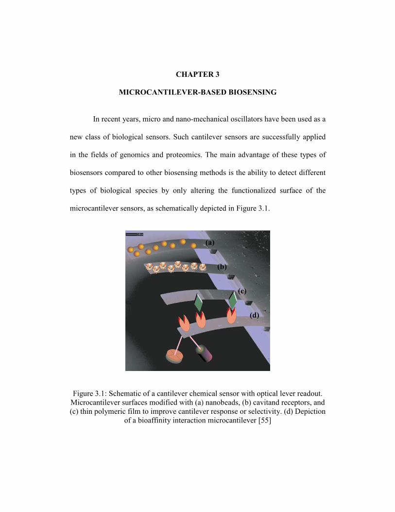
MICROCANTILEVER-BASED BIOSENSING

In recent years, micro and nano-mechanical oscillators have been used as a

new class of biological sensors. Such cantilever sensors are successfully applied

in the fields of genomics and proteomics. The main advantage of these types of

biosensors compared to other biosensing methods is the ability to detect different

types of biological species by only altering the functionalized surface of the

microcantilever sensors, as schematically depicted in Figure 3.1.

Figure 3.1: Schematic of a cantilever chemical sensor with optical lever readout.

Microcantilever surfaces modified with (a) nanobeads, (b) cavitand receptors, and

(c) thin polymeric film to improve cantilever response or selectivity. (d) Depiction

of a bioaffinity interaction microcantilever [55]

(a)

(b)

(c)

(d)

14

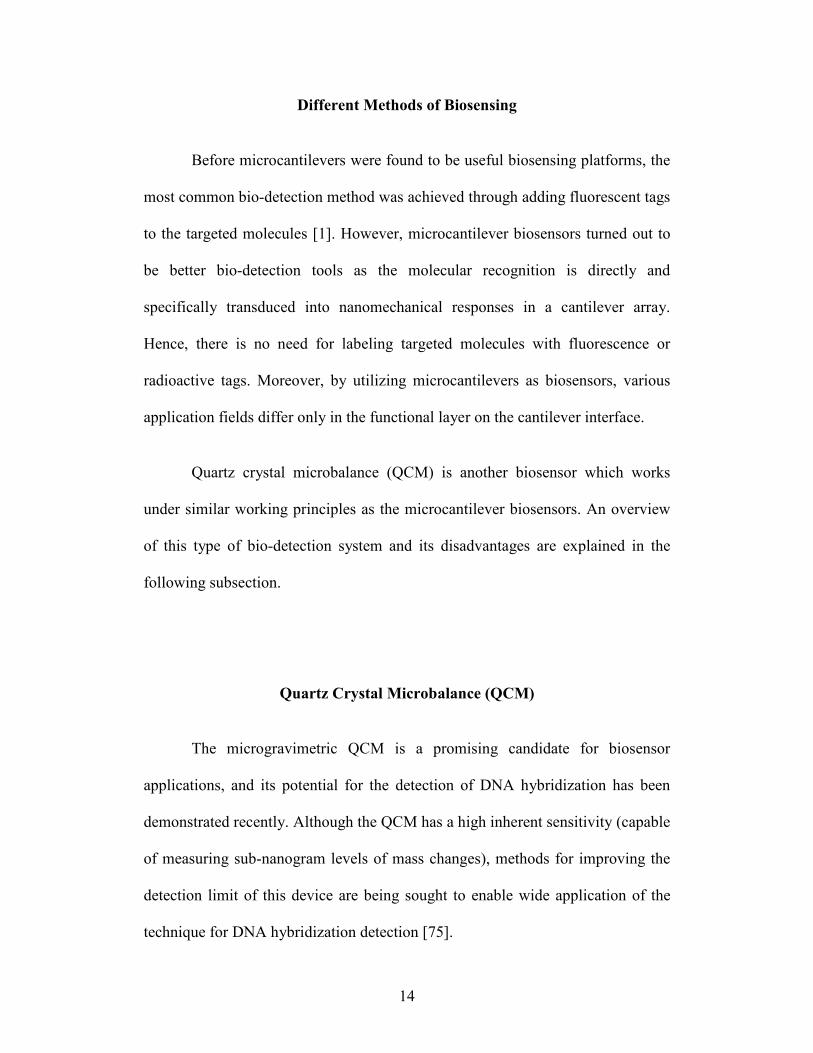
Different Methods of Biosensing

Before microcantilevers were found to be useful biosensing platforms, the

most common bio-detection method was achieved through adding fluorescent tags

to the targeted molecules [1]. However, microcantilever biosensors turned out to

be better bio-detection tools as the molecular recognition is directly and

specifically transduced into nanomechanical responses in a cantilever array.

Hence, there is no need for labeling targeted molecules with fluorescence or

radioactive tags. Moreover, by utilizing microcantilevers as biosensors, various

application fields differ only in the functional layer on the cantilever interface.

Quartz crystal microbalance (QCM) is another biosensor which works

under similar working principles as the microcantilever biosensors. An overview

of this type of bio-detection system and its disadvantages are explained in the

following subsection.

Quartz Crystal Microbalance (QCM)

The microgravimetric QCM is a promising candidate for biosensor

applications, and its potential for the detection of DNA hybridization has been

demonstrated recently. Although the QCM has a high inherent sensitivity (capable

of measuring sub-nanogram levels of mass changes), methods for improving the

detection limit of this device are being sought to enable wide application of the

technique for DNA hybridization detection [75].

15

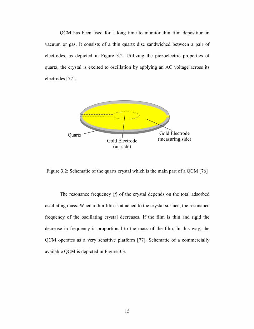
QCM has been used for a long time to monitor thin film deposition in

vacuum or gas. It consists of a thin quartz disc sandwiched between a pair of

electrodes, as depicted in Figure 3.2. Utilizing the piezoelectric properties of

quartz, the crystal is excited to oscillation by applying an AC voltage across its

electrodes [77].

Figure 3.2: Schematic of the quarts crystal which is the main part of a QCM [76]

The resonance frequency (f) of the crystal depends on the total adsorbed

oscillating mass. When a thin film is attached to the crystal surface, the resonance

frequency of the oscillating crystal decreases. If the film is thin and rigid the

decrease in frequency is proportional to the mass of the film. In this way, the

QCM operates as a very sensitive platform [77]. Schematic of a commercially

available QCM is depicted in Figure 3.3.

Quartz

Gold Electrode

(air side)

Gold Electrode

(measuring side)

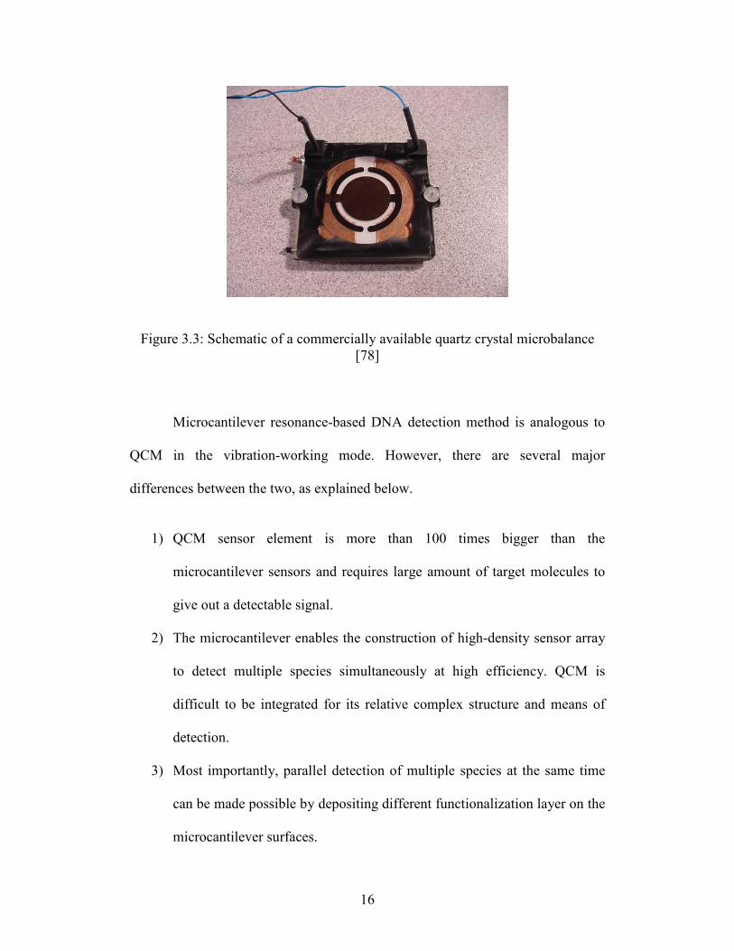
16

Figure 3.3: Schematic of a commercially available quartz crystal microbalance

[78]

Microcantilever resonance-based DNA detection method is analogous to

QCM in the vibration-working mode. However, there are several major

differences between the two, as explained below.

1) QCM sensor element is more than 100 times bigger than the

microcantilever sensors and requires large amount of target molecules to

give out a detectable signal.

2) The microcantilever enables the construction of high-density sensor array

to detect multiple species simultaneously at high efficiency. QCM is

difficult to be integrated for its relative complex structure and means of

detection.

3) Most importantly, parallel detection of multiple species at the same time

can be made possible by depositing different functionalization layer on the

microcantilever surfaces.

17

Microcantilever Biosensors Modes of Detection

A microcantilever biosensor can be operated in the following two different

modes:

Static mode: In this mode, the deflection of the microcantilever beam is

measured. Having the deflection of the beam after the adsorption of biological

species, adsorption induced surface stress can be accordingly calculated.

Dynamic mode: In this mode, the shift in resonance frequency of the beam

is measured. Knowing the shift of resonance frequency after the adsorption, the

adsorption induced surface stress and/or the added mass can be calculated.

Various mathematical models have been developed to explain the two

modes of microcantilever operation. Some of them are described in the following

subsections.

Static Mode

Long before the first microfabricated cantilevers were created, changes in

surface stresses of these systems had been studied by measuring minute

deformations of relatively thin (up to 1 mm) plates, referred to as the “beam-

bending” technique. Koch and Abermann demonstrated that the bending of a

cantilever can be measured with sufficient sensitivity that the change in the stress

due to the deposition of a single monolayer on one side can be detected [34].

18

This technique was first proposed by Stoney in 1909 to measure the

residual stresses in metallic thin films deposited by electrolysis [59]. In this

method, the surface stress is calculated from the observed deformation of the

rectangular plate using the following simple equation, which is commonly

referred to as Stoney’s formula:

( )σ

υEt

Lz

2

213 −= (3.1)

where z is the displacement of the cantilever, υ , L, t and E are the Poisson’s ratio,

length, thickness and modulus of elasticity of the cantilever, respectively, and σ

is the adsorption-induced differential surface stress.

The Stoney’s formula is applicable to thin plates with uniform thickness

exhibiting small deflections, where the effect of in-plane loading on the transverse

(out-of-plane) deflections is negligible.

Corrections to the Stoney’s Formula

In the ‘‘thin-film approximation’’ considered in Stoney’s formula, that is,

in the case of a thin film (coating) on a thick substrate, the average stress or

macrostress acting in the coating ( cσ ) can be expressed in a very simple manner

as [32]

0

' εσ ∆≅ cc E (3.2)

19

where '

cE is the biaxial modulus of the coating (υ−

=1

' EE ) and 0ε∆ characterizes

the strain mismatch between coating and the substrate ( 0,0,0 sc εεε −=∆ ).

However, in order to extend the Stoney’s formula to the case of “thick” films, the

general theory of elastic interactions in multilayer laminates [67] must be used

instead of Eq. (3.2), which can be best expressed as [33]

−−

++∆

+= Kz

tt

tEtE

tEEz cs

ccss

ss

cc θεσ2

)( 0''

'

' (3.3)

where z is measured from the bottom surface of the substrate, K is the curvature,

st and ct are the thickness of substrate and coating, respectively, and the parameter

θ is defined as follows

( )( )ccss

cscs

tEtE

EEtt''

''

2 +

−=θ (3.4)

By defining parameters '

'

1

s

c

E

E=γ and

s

c

t

t=δ , the ratio of the corrected

average stress intensity in the coating ( cσ ) to that calculated by Stoney’s formula

( stσ ) is simply found to be [32]

δδγ

σσ

+

+=

1

1 3

1

st

c (3.5)

which emphasizes that, in fact, it is a straightforward matter to extend Stoney’s

equation to situations involving thick coatings.

20

Based on Eq. (3.5), it is shown that Stoney’s original formula does not

cause serious errors for thickness ratios of 1.0≤δ , but fails to properly describe

the variation of stress with thickness and cannot be relied upon for thickness

ratios of 1.0>δ [32]. In the absence of information on the biaxial modulus of the

coating, Atkinson’s approximation can be applied [3]. It considers a correction

factor equal to δ+1

1 for the Stoney’s formula, resulting in

δσ

σ+

=1

stAt .

Atkinson’s approximation yields much better results (compared to Stoney’s

formula) and can be used for thickness ratios up to about 40%.

Uniform Curvature Assumption and Modeling the Surface Stress

The original Stoney’s equation assumes that surface stress is uniformly

changed during the deflection and relates the surface stress to the radius of

curvature of the cantilever, R, as [64]

( )σ

υ2

161

EtR

−= (3.6)

This formula assumes a uniform curvature for the whole deflected

structure which is quite extreme for the nonlinear analysis of film large deflection

and its limitation is illustrated in [32] and [19].

The uniform curvature assumption is identical to modeling the cantilever

under the surface stress as an unrestrained (free) plate, which violates the clamp

21

boundary condition of the “cantilever” at x=0. In other words, the Stoney’s

equation describes the surface stress-induced deformation of a cantilever plate

only if; 1) the length of the plate greatly exceeds its width, and 2) the point under

consideration is far from the clamp. Another characteristic of the Stoney’s

formula in the modeling of the problem is to replace the adsorption-induced

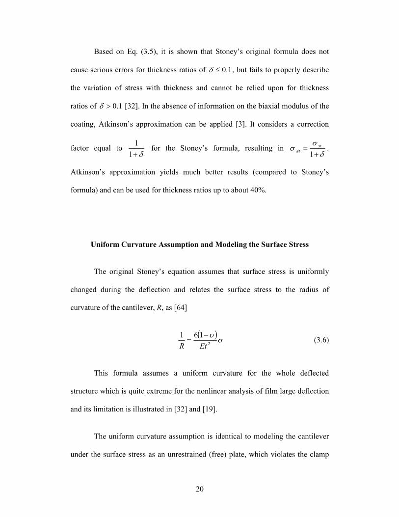
surface stress as a moment applied at the structure’s free end. Considering both

these assumptions and their shortcomings, Sader has improved the plate’s

modeling by replacing the differential surface stress σ∆ applied to the faces of

the plate by moments per unit length of magnitude 2/tσ∆ loaded at the free

edges of the plate, as depicted in Figure 3.4, where t is the thickness of the plate

[51]. The clamped end boundary condition is also considered in Sader’s

formulation. Since an exact analytical solution for a cantilever plate is extremely

difficult, if not impossible to obtain, finite element method is utilized to obtain a

qualitative overview of the cantilever plate’s behavior. An approximate analytical

formula is also derived to replace the Stoney’s formula in situations where it is

found to be inaccurate.

22

Figure 3.4: Schematic diagram showing loading of free edges of cantilever plate

by moments per unit length 2/tM app σ∆= [51]

In order to improve the modeling of the cantilever, the adsorption-induced

surface stress can be replaced by a moment (similar to Stoney’s and Sader’s

formulation) together with a concentrated transverse load applied at the free end

of the cantilever [43]

None of these analyses that model the surface stress as a moment (or

moment together with force) applied at the structure’s free edge or free end, take

the influence of the surface stress on structure stiffness into account. This may be

improved by modeling the applied surface stress as an area stress which is

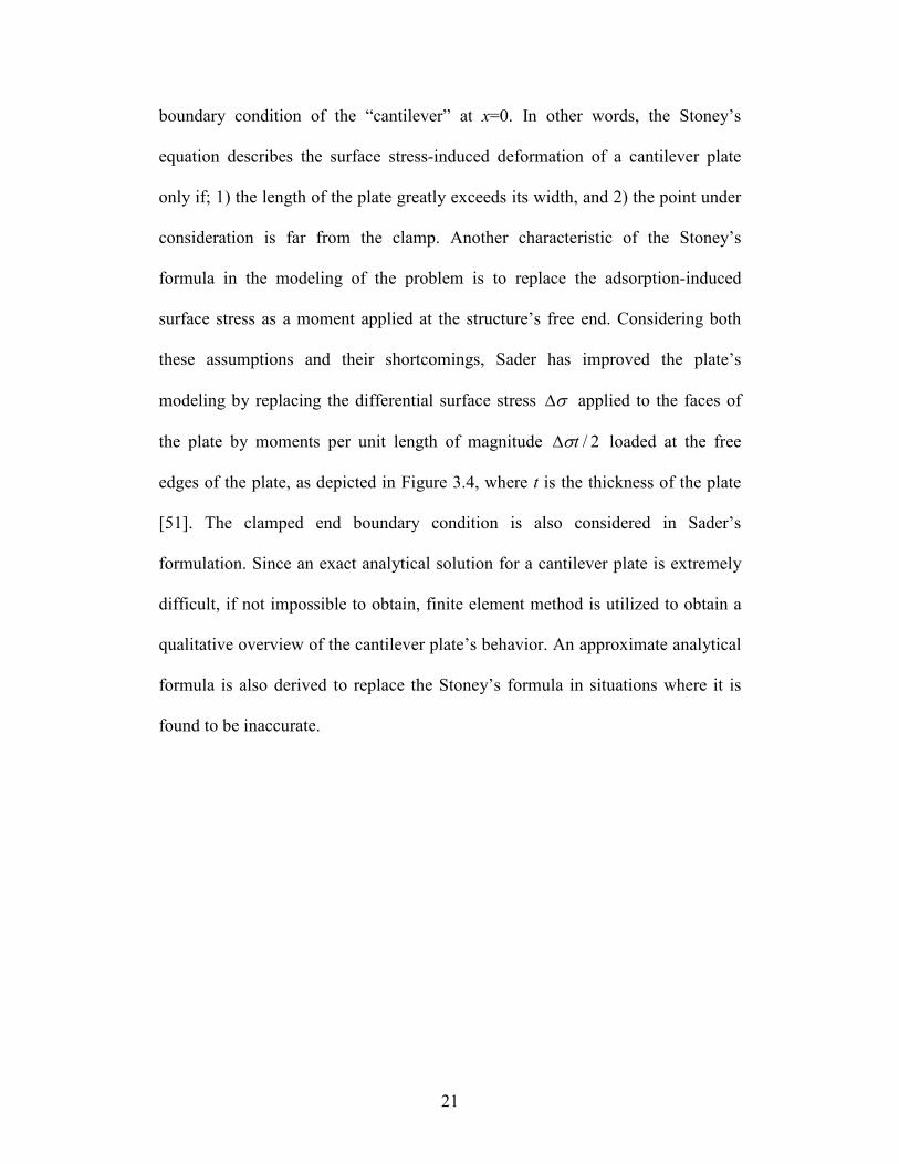
uniformly distributed on the upper surface of the beam, as depicted in Figure 3.5

[13, 74]. Applying the principle of virtual work, the equation of motion of the

beam and the boundary conditions can then be derived. Utilizing this modeling, it

is demonstrated how the stiffening effect of tensile stress becomes important

when the magnitude of the surface stress becomes relatively large [74].

23

Figure 3.5: Schematic of the uniformly distributed surface stress model [74]

Static Deflection based on Energy Dissipation

It is well established that molecular adsorption changes the surface free

energy of a substrate surface due to the fact that all binding reactions are driven

by the reduction of free energy, as mentioned in Chapter 2. The Shuttleworth

equation was also given in Eq. (2.1) relating the surface stress and the surface free

energy, as rewritten below,

AA∂∂

+=γ

γσ (3.7)

However, the Shuttleworth equation is somewhat difficult to apply to

Stoney’s formula (or any of its modified versions) since the second term in Eq.

(3.7) (i.e.A∂∂γ

) depends on beam curvature, which is an unknown. Hence, both the

Stoney and Shuttleworth equations must be solved simultaneously to obtain σ

and z (the deflection of the microcantilever beam). Ibach has carefully studied the

surface stress on crystalline cantilevers induced by adsorption of single atoms

[27]. However, when dealing with complex molecules like proteins, as it is often

24

the case in biochemical sensing, there are several other possible sources of stress

rather than simple ion adsorption onto a clean crystal surface.

Electrostatic interaction between neighboring adsorbed species, changes in

surface hydro-phobicity, and conformational changes of the adsorbed molecules

can all induce stresses which may contrast with each other and make the change

in stress not directly related to the receptor-ligand binding energy or the rupture

force. As an example, it has been recently observed how adsorption of

complementary single-stranded DNA onto the cantilever surface can induce either

compressive or tensile stress depending on the ionic strength of the buffer in

which the hybridization takes place [75]. This behavior is interpreted as the

interplay between two opposite driving forces; reduction of the configurational

entropy of the adsorbed DNA after hybridization which tends to lower the

compressive stress, and intermolecular electrostatic repulsion between adsorbed

DNA which tends to increase the compressive stress.

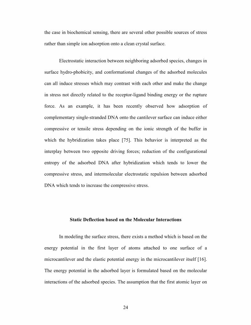
Static Deflection based on the Molecular Interactions

In modeling the surface stress, there exists a method which is based on the

energy potential in the first layer of atoms attached to one surface of a

microcantilever and the elastic potential energy in the microcantilever itself [16].

The energy potential in the adsorbed layer is formulated based on the molecular

interactions of the adsorbed species. The assumption that the first atomic layer on

25

the beams surface plays a dominate role in microcantilever deflections is

supported by the experimental works of Martinez et al. [41] and Schell-Sorokin et

al. [54] who measured changes in curvature in cantilevered-thin plates due to

adsorption of submonolayer of different atoms in ultrahigh vacuum conditions.

Regarding this assumption, the arrangement of adsorbed atoms (or molecules) on

the surface of microcantilever is modeled as shown in Figure 3.6.

Figure 3.6: Arrangement of atoms (or molecules) on cantilever surface

According to the proposed model, atoms in the attached film are attracted

and repulsed according to the Lennard–Jones potential formula

126)(

r

B

r

Arw +

−= (3.8)

where r is the spacing between atoms (molecules) and A and B are Lennard–Jones

constants. Part of this potential is transferred into the cantilever as elastic strain

energy causing the beam to deflect. The equilibrium configuration of the

cantilever is determined by minimizing the total potential function, which is made

up of the Lennard–Jones potential and the elastic energy in the cantilever. By

considering a simple model of the curved beam (after the bending of the

26

microcantilever) as depicted in Figure 3.7, the total atomic and elastic bending

potential energy is found to be

( ) ( ) ( )[ ] ( )[ ]b

REI

azb

B

azb

A

zb

B

zb

AUUU bs

2

6223

22126

1

2

1

4/14/12

+

+−+

+−

−+

−+

−

−=+=

(3.9)

where R is the radius of curvature and a and b are parameters shown in Figures

3.6 and 3.7.

Figure 3.7: Position of surface atoms (or molecules) on the deflected

microcantilever beam [16]

In order to find the radius of curvature of the deflected beam, and hence

the deflection of the beam, the amount of U in Eq. (3.9) must be a relative

minimum, which is determined from [16]

0dU

cd

R

=

(3.10)

27

Remark: Instead of the Lennard-Jones formula used in deriving Us, the

simpler van der Waals potential [Eq. (3.11)] may be used

6r

CU s −= (3.11)

where the interaction constant C can be determined as C = 1.05×10−76cd (Jm

6 ),

where c and d are van der Waals constants depending on the type of atoms

(molecules) [16].

Dynamic Mode

Contrary to static mode, there exist different models for analyzing the

effect of the adsorption induced surface stress on the resonance frequency shift of

the microcantilever. Some of these models are explained in the following

subsections.

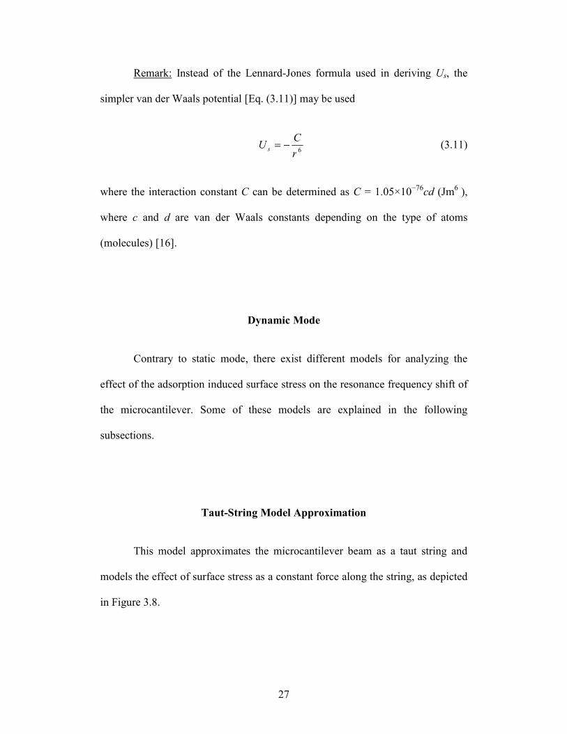
Taut-String Model Approximation

This model approximates the microcantilever beam as a taut string and

models the effect of surface stress as a constant force along the string, as depicted

in Figure 3.8.

28

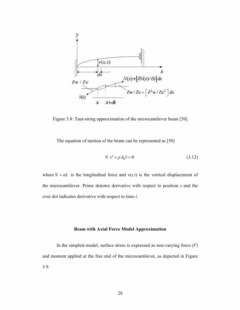
Figure 3.8: Taut-string approximation of the microcantilever beam [50]

The equation of motion of the beam can be represented as [50]

0bN v A v+ =′′ ρ ɺɺ (3.12)

where LN σ= is the longitudinal force and v(s,t) is the vertical displacement of

the microcantilever. Prime denotes derivative with respect to position s and the

over dot indicates derivative with respect to time t.

Beam with Axial Force Model Approximation

In the simplest model, surface stress is expressed as non-varying force (F)

and moment applied at the free end of the microcantilever, as depicted in Figure

3.9.

29

Figure 3.9: Schematic view of a microcantilever with uniform surface stress

Having this force, the equation of motion of the microcantilever beam can

be expressed as [39]

0bEI v Fv A v− + =′′′′ ′′ ρ ɺɺ (3.13)

This model was later modified by assuming that the axial force due to

surface stress varies along the microcantilever and the surface stress exists only

on a fraction of the microcantilever as depicted in Figure 3.10.

Figure 3.10: Microcantilever with fractional surface stresses coverage

This assumption modifies the equation of motion of the beam as follows

[50]

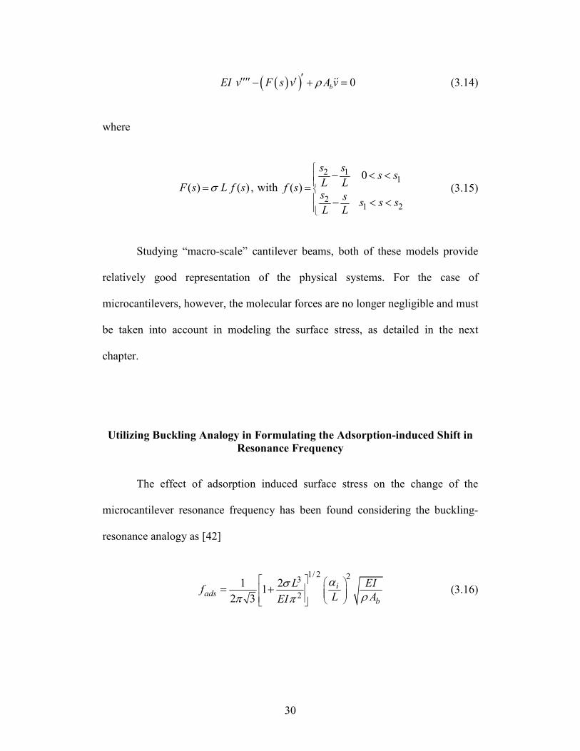
30

( )( ) 0bEI v F s v A v′′′′′ ′− + =ɺɺρ (3.14)

where

2 11

21 2

0( ) ( ) , with ( )

s ss s

L LF s L f s f ss s

s s sL L

σ

− < <= =

− < < (3.15)

Studying “macro-scale” cantilever beams, both of these models provide

relatively good representation of the physical systems. For the case of

microcantilevers, however, the molecular forces are no longer negligible and must

be taken into account in modeling the surface stress, as detailed in the next

chapter.

Utilizing Buckling Analogy in Formulating the Adsorption-induced Shift in Resonance Frequency

The effect of adsorption induced surface stress on the change of the

microcantilever resonance frequency has been found considering the buckling-

resonance analogy as [42]

1/ 2 23

2

1 21

2 3

iads

b

L EIf

L AEI

ασρπ π

= + (3.16)

31

where ρ and Ab are the mass density and cross-sectional area of the

microcantilever, respectively, and αi is the i-th positive root of the eigenfrequency

equation

01coshcos =+ii αα (3.17)

As the resonance frequency of the microcantilever beam can be easily

found from the general equation of motion of the vibrating beam, the main effort

has been done in formulating the surface stress (and its effects) into the equation

of motion of the microcantilever.

Recent Developments in Microcantilever Biosensors

Sensitivity Enhancement

Physical dimensions play an important role in the sensitivity of

microcantilever sensors for mass detection. Modeling the microcantilever as a

simple 1D oscillator, its natural frequency may be formulated as follows [13]

1

2 b

Kf

m=

π (3.18)

where K is the spring constant and bm =n beamm is the effective beam mass with

beamm being it’s actual mass and n being a geometric parameter accounting for

32

the non point-mass distribution. n has a typical value of 0.24 for a rectangular

microcantilever beam.

Presence of mass on the microcantilever surface results in the generation

of differential surface stress. This changes the spring constant, which in turn

changes the natural frequency. In general, the altered resonance frequency can be

formulated as follows [13]

1

2 b

K Kf

m n m

+=

+δ

δπ δ

(3.19)

where Kδ is the change in the spring constant attributed to adsorption induced

surface stress and mδ being the added mass.

It has been shown that if adsorption is localized (i.e., end loading), the

change in resonance frequency due to change in spring constant can be neglected.

If the spring constant K can be formulated as follows [64]

3

34

EbhK

L= (3.20)

with E being the Young’s modulus of elasticity for the microcantilever beam

material and , , and b h L being width, thickness and length of the beam,

respectively. Then, the resonance frequency f of the microcantilever beam can be

given as follows [64]

33

2

1

22 (0.98) eq

h E Kf

mL= =

ρ ππ (3.21)

where eqm is the equivalent mass consisting of mass of microcantilever beam and

adsorbed mass. If dm is the mass added at the end of the microcantilever beam,

then eqm = dnm + bm .

The shifted resonance frequency fδ can be given by [64]

3

3

1

2 4 ( )d

Ebhf

nL m bhLδ π ρ=

+ (3.22)

The adsorbed mass mδ can then be determined from the change in the

resonance frequency using the following equation [64]

2 2

2

f f m

f m

δ δ−= (3.23)

The mass sensitivity mS of the sensor can be given by [64]

0

1 1, limm

ms

f df mS m

f m f dm A

δ∆ →

∆= = ∆ =

∆ (3.24)

where sA is the active area of the sensor. The sensitivity is the fractional change

in resonant frequency with addition of mass to the sensor. When applied to the

microcantilever sensor, the sensitivity can be expressed as follows [64]

34

1

1 d

1 for distributed load

for end load2 ( 0.24 )

mSh

h h

ρζ

ρ ζ

=

−=

+

(3.25)

where 1ζ and dh are the fractional area coverage and thickness of the deposited

mass at the end loaded microcantilever beam. The minimum detectable mass

minm∆ can be given by the following equation [64]

f

f

Sm

m

minmin

1 ∆=∆ (3.26)

Reduction in dimensions can lead to improvement in sensitivity of

resonance mode of the mass sensors. However, size reduction leads to different

sensor fabrication difficulties. Several different methods have been explored to

improve sensitivity without having to reduce the microcantilever dimensions

further. One of the most recent one of these presents a method of increasing the

sensitivity by using a frequency tuning approach to measure mass changes. The

method uses a closed loop strategy to measure mass change in parametric

resonance based sensor. A DC offset is applied to the sensor as a feedback signal

to compensate for the frequency shift at the boundary of the parametric resonance

region. Mass changes are detected by measuring the DC offset feedback [73].

35

Potential and Practical Medical Applications

Microcantilever biosensors are useful platforms for different medical

diagnostics. They have been successfully used in DNA detection [23, 60, 71]. The

sensing or detection of DNA strands is important in the fabrication of DNA probe

arrays useful in DNA sequencing or gene mapping applications [23]. A schematic

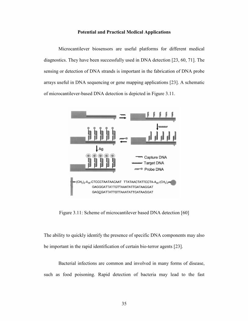
of microcantilever-based DNA detection is depicted in Figure 3.11.

Figure 3.11: Scheme of microcantilever based DNA detection [60]

The ability to quickly identify the presence of specific DNA components may also

be important in the rapid identification of certain bio-terror agents [23].

Bacterial infections are common and involved in many forms of disease,

such as food poisoning. Rapid detection of bacteria may lead to the fast

36

adjustment of antibiotic treatment, which in turn leads to decreased mortality and

lowers the hospitalization cost [21].

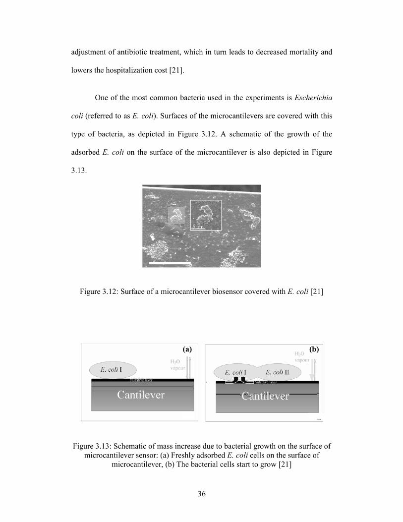
One of the most common bacteria used in the experiments is Escherichia

coli (referred to as E. coli). Surfaces of the microcantilevers are covered with this

type of bacteria, as depicted in Figure 3.12. A schematic of the growth of the

adsorbed E. coli on the surface of the microcantilever is also depicted in Figure

3.13.

Figure 3.12: Surface of a microcantilever biosensor covered with E. coli [21]

Figure 3.13: Schematic of mass increase due to bacterial growth on the surface of

microcantilever sensor: (a) Freshly adsorbed E. coli cells on the surface of

microcantilever, (b) The bacterial cells start to grow [21]

(a) (b)

37

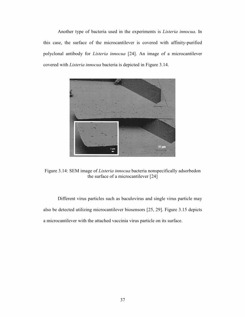
Another type of bacteria used in the experiments is Listeria innocua. In

this case, the surface of the microcantilever is covered with affinity-purified

polyclonal antibody for Listeria innocua [24]. An image of a microcantilever

covered with Listeria innocua bacteria is depicted in Figure 3.14.

Figure 3.14: SEM image of Listeria innocua bacteria nonspecifically adsorbedon

the surface of a microcantilever [24]

Different virus particles such as baculovirus and single virus particle may

also be detected utilizing microcantilever biosensors [25, 29]. Figure 3.15 depicts

a microcantilever with the attached vaccinia virus particle on its surface.

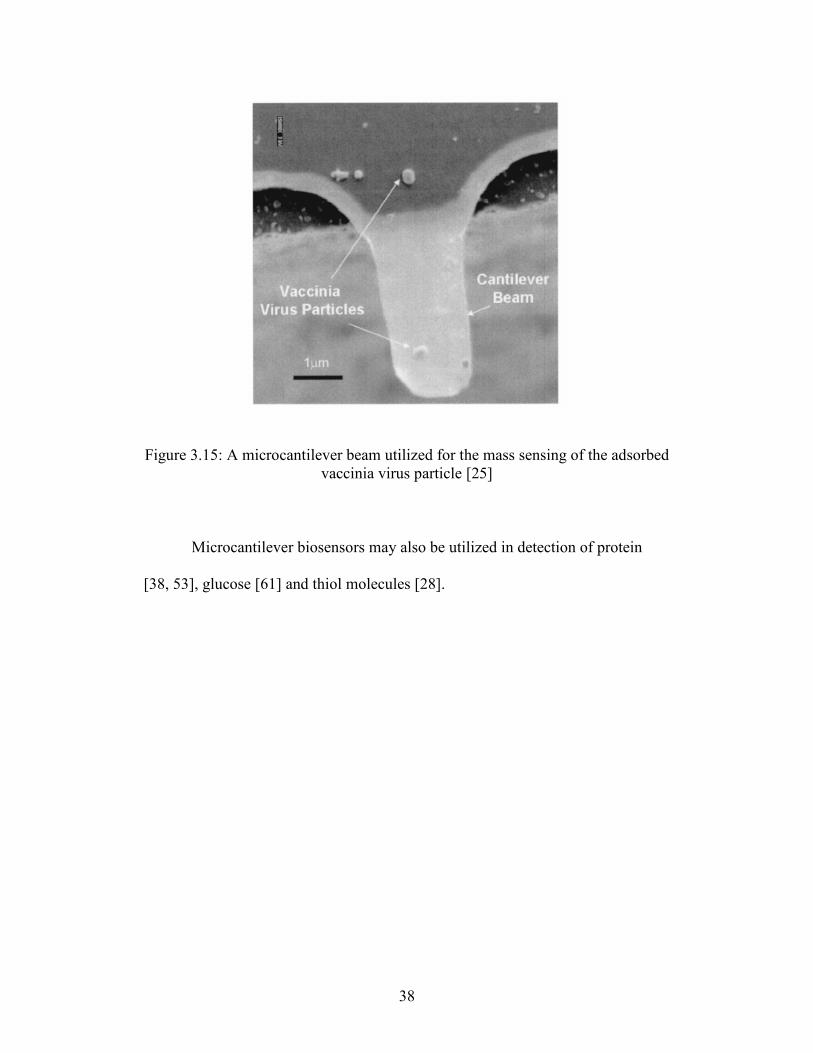
38

Figure 3.15: A microcantilever beam utilized for the mass sensing of the adsorbed

vaccinia virus particle [25]

Microcantilever biosensors may also be utilized in detection of protein

[38, 53], glucose [61] and thiol molecules [28].

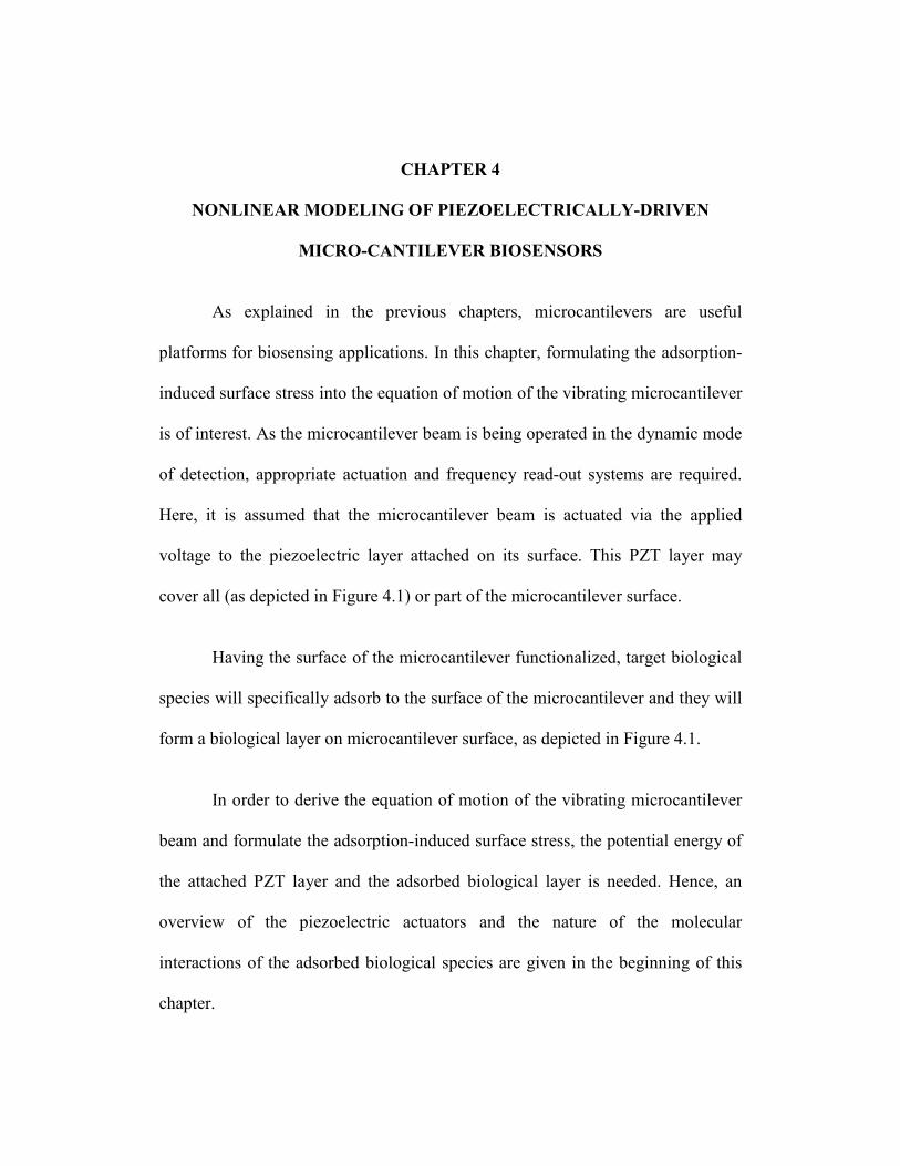
CHAPTER 4

NONLINEAR MODELING OF PIEZOELECTRICALLY-DRIVEN

MICRO-CANTILEVER BIOSENSORS

As explained in the previous chapters, microcantilevers are useful

platforms for biosensing applications. In this chapter, formulating the adsorption-

induced surface stress into the equation of motion of the vibrating microcantilever

is of interest. As the microcantilever beam is being operated in the dynamic mode

of detection, appropriate actuation and frequency read-out systems are required.

Here, it is assumed that the microcantilever beam is actuated via the applied

voltage to the piezoelectric layer attached on its surface. This PZT layer may

cover all (as depicted in Figure 4.1) or part of the microcantilever surface.

Having the surface of the microcantilever functionalized, target biological

species will specifically adsorb to the surface of the microcantilever and they will

form a biological layer on microcantilever surface, as depicted in Figure 4.1.

In order to derive the equation of motion of the vibrating microcantilever

beam and formulate the adsorption-induced surface stress, the potential energy of

the attached PZT layer and the adsorbed biological layer is needed. Hence, an

overview of the piezoelectric actuators and the nature of the molecular

interactions of the adsorbed biological species are given in the beginning of this

chapter.

40

Figure 4.1: Schematic of a microcantilever biosensor with the attached biological

species and the piezoelectric layer on its surface

Piezoelectric Actuators

The piezoelectric effect was discovered in 1880 [2]. The ability of certain

crystalline materials (ceramics) to generate an electrical charge in proportion of

an externally applied force is called direct piezoelectric field. This direct effect is

used in force transducers. According to the inverse piezoelectric effect, an electric

field parallel to the direction of polarization induces an expansion of the ceramic.

The direction of expansion with respect to the direction of the electrical field

depends on the constants appearing in the constitutive equations. The material can

be manufactured in such a way that one of the coefficients dominates the others.

One of the materials most frequently used for piezoelectric actuators is lead-

zirconium-titanate, or PZT [2]. From here on, PZT is used to refer to the

piezoelectric actuator unless otherwise stated.

Piezoelectric

Layer

Biological

Layer

41

For the inverse piezoelectric effect, the electrical and mechanical

constitutive equations are coupled as follows [2]:

ES s T dE= + (4.1)

where constant d (with the dimension of C/N or m/V) relates the strain to the

electric field E (with the dimension of V/m) in the absence of mechanical stress

and sE (having dimension of m

2/N) refers to the compliance when the electric

field is constant. S and T are the strain and stress vectors with dimensions of

(m/m) and (N/m2), respectively.

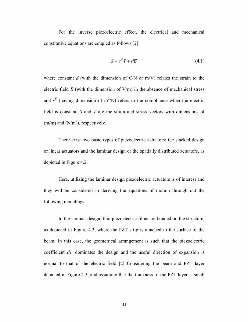
There exist two basic types of piezoelectric actuators: the stacked design

or linear actuators and the laminar design or the spatially distributed actuators, as

depicted in Figure 4.2.

Here, utilizing the laminar design piezoelectric actuators is of interest and

they will be considered in deriving the equations of motion through out the

following modelings.

In the laminar design, thin piezoelectric films are bonded on the structure,

as depicted in Figure 4.3, where the PZT strip is attached to the surface of the

beam. In this case, the geometrical arrangement is such that the piezoelectric

coefficient d31 dominates the design and the useful direction of expansion is

normal to that of the electric field [2] Considering the beam and PZT layer

depicted in Figure 4.3, and assuming that the thickness of the PZT layer is small

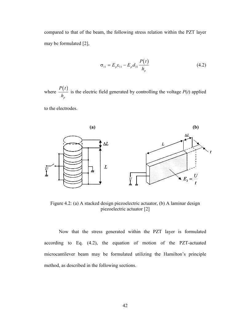
42

compared to that of the beam, the following stress relation within the PZT layer

may be formulated [2],

( )11 11 31p p

p

P tE E d

hσ = ε − (4.2)

where ( )p

P t

h is the electric field generated by controlling the voltage P(t) applied

to the electrodes.

Figure 4.2: (a) A stacked design piezoelectric actuator, (b) A laminar design

piezoelectric actuator [2]

Now that the stress generated within the PZT layer is formulated

according to Eq. (4.2), the equation of motion of the PZT-actuated

microcantilever beam may be formulated utilizing the Hamilton’s principle

method, as described in the following sections.

(a) (b)

43

Figure 4.3: PZT strip bonded to the surface of a beam [2]

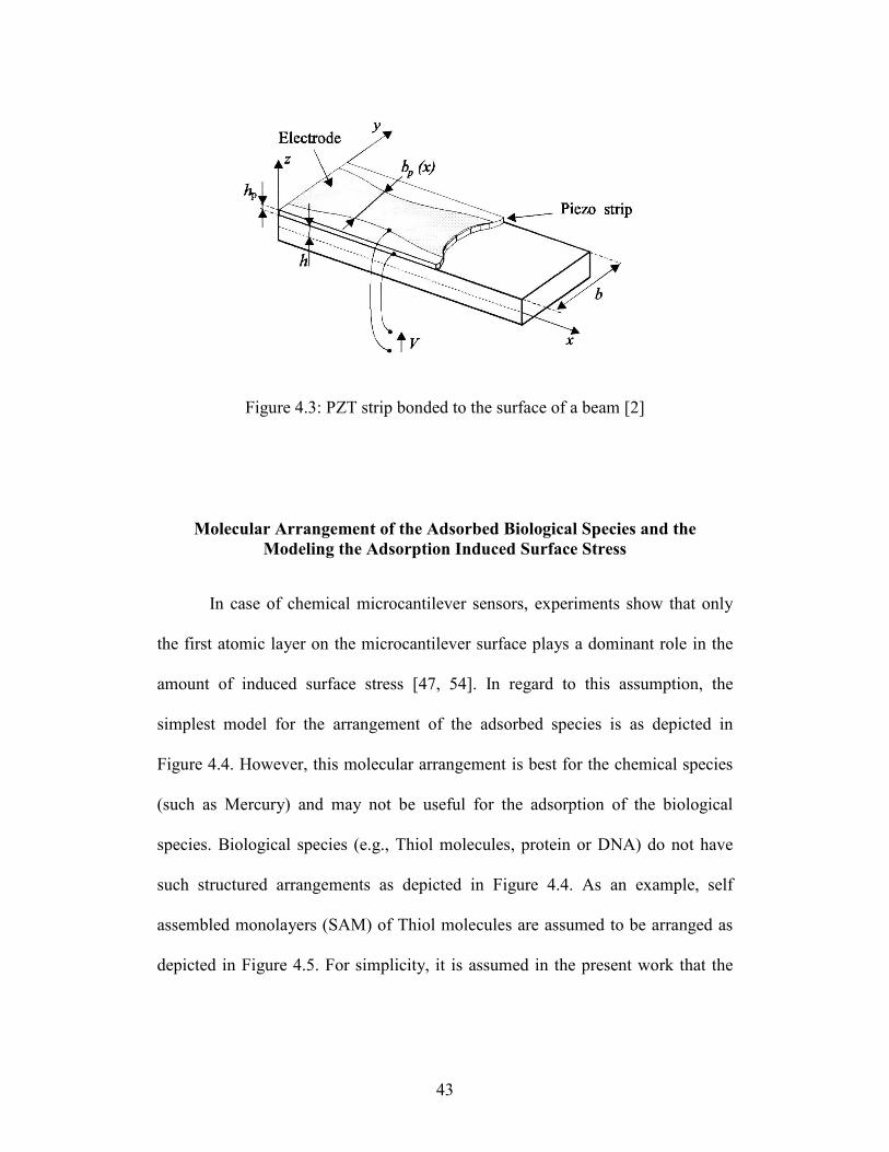
Molecular Arrangement of the Adsorbed Biological Species and the Modeling the Adsorption Induced Surface Stress

In case of chemical microcantilever sensors, experiments show that only

the first atomic layer on the microcantilever surface plays a dominant role in the

amount of induced surface stress [47, 54]. In regard to this assumption, the

simplest model for the arrangement of the adsorbed species is as depicted in

Figure 4.4. However, this molecular arrangement is best for the chemical species

(such as Mercury) and may not be useful for the adsorption of the biological

species. Biological species (e.g., Thiol molecules, protein or DNA) do not have

such structured arrangements as depicted in Figure 4.4. As an example, self

assembled monolayers (SAM) of Thiol molecules are assumed to be arranged as

depicted in Figure 4.5. For simplicity, it is assumed in the present work that the

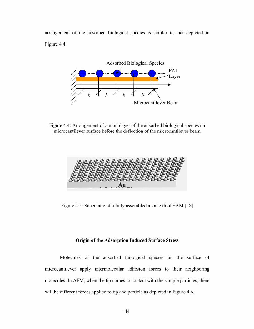
44

arrangement of the adsorbed biological species is similar to that depicted in

Figure 4.4.

Figure 4.4: Arrangement of a monolayer of the adsorbed biological species on

microcantilever surface before the deflection of the microcantilever beam

Figure 4.5: Schematic of a fully assembled alkane thiol SAM [28]

Origin of the Adsorption Induced Surface Stress

Molecules of the adsorbed biological species on the surface of

microcantilever apply intermolecular adhesion forces to their neighboring

molecules. In AFM, when the tip comes to contact with the sample particles, there

will be different forces applied to tip and particle as depicted in Figure 4.6.

b b b b

Adsorbed Biological Species

PZT

Layer

Microcantilever Beam

45

Figure 4.6: The interacting forces between tip and nanoparticles in AFM

positioning [57]

Repulsive contact forces, Aas and Ata are the adhesion forces. The main

components of these adhesion forces are van der Waals, capillary, and

electrostatic forces [57].

In microcantilever sensing method, the only forces present are adhesion

ones. In this section, the presence of different types of adhesion forces in

biosensing microcantilevers are verified, and tried to be formulated.

Intermolecular Forces of Attraction and Repulsion

Considering the chemical microcantilever sensors, the arrangement of the

first layer of the adsorbed species (e.g., mercury) may be simply modeled as

depicted in Figure 4.7.

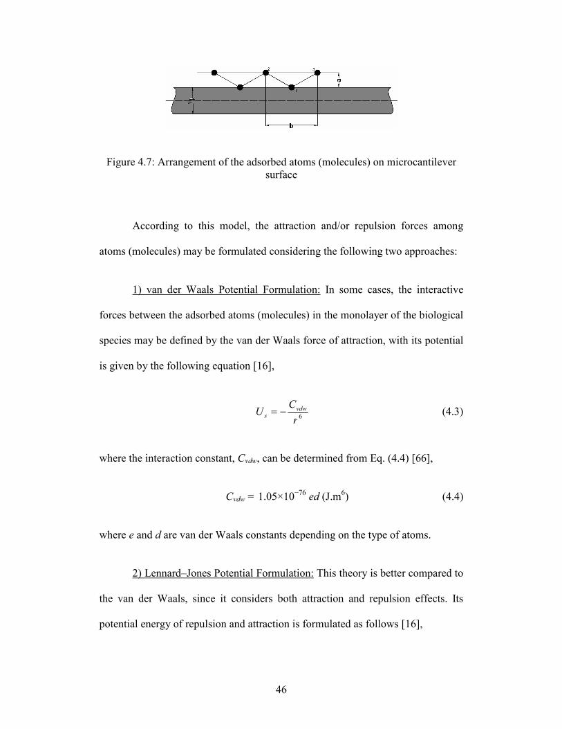
46

Figure 4.7: Arrangement of the adsorbed atoms (molecules) on microcantilever

surface

According to this model, the attraction and/or repulsion forces among

atoms (molecules) may be formulated considering the following two approaches:

1) van der Waals Potential Formulation: In some cases, the interactive

forces between the adsorbed atoms (molecules) in the monolayer of the biological

species may be defined by the van der Waals force of attraction, with its potential

is given by the following equation [16],

6r

CU vdw

s −= (4.3)

where the interaction constant, Cvdw, can be determined from Eq. (4.4) [66],

Cvdw = 1.05×10−76

ed (J.m6) (4.4)

where e and d are van der Waals constants depending on the type of atoms.

2) Lennard–Jones Potential Formulation: This theory is better compared to

the van der Waals, since it considers both attraction and repulsion effects. Its

potential energy of repulsion and attraction is formulated as follows [16],

47

6 12( )

A Bw r

r r

−= + (4.5)

where r is the spacing between atoms (molecules) and A and B are the Lennard–

Jones constants depending on the types of molecules. These constants are

available for individual atoms and simple molecules. However, it is not an easy

and straight forward procedure to obtain the Lennard-Jones constants for complex

molecules and biological species such as protein.

Lennard-Jones Constants of A and B

In case of having two atoms, the Lennard-Jones constants of attraction/

repulsion is found to be as A=10-77Jm

6 and B=10

-134Jm

12. However, in general, in

order to find the Lennard-Jones constants, we should follow the steps described

bellow:

In general, the Lennard-Jones potential is formulated using the following

equation [72],

12 6

( ) 4w rr r

σ σε = −

(4.6)

where ε is a parameter determining the depth of the potential well and σ is a

length scale parameter that determines the position of the potential minimum and

is defined as follows [72],

48

1/ 62 Nr−σ = (4.7)

in which rN is the nearest neighboring distance in the atomic structure. For FCC

(face-centered cubic), BCC (body-centered cubic) and diamond crystal structures,

rN equals 2 / 2a , 3 / 2a , and 3 / 4a respectively, where a is the lattice

constant of the specific crystal. The value for parameter a is given in Table 4.1 for

some elements.

where z0 is the equilibrium distance between the two contact planes

(

1/ 6

0

2

15z σ =

) [72].

Once σ is known, ∆γ (the work done to move two surfaces from

equilibrium separation z0 to infinity) could be readily obtained from tabulated

handbook values or from measurement. Thus, the second parameter of the

interatomic Lennard–Jones potential, ε, could be obtained from the following

equation [72]:

1

016

A

zγ

π∆ = (4.8)

where

2 6

1 1 24A επ ρ ρ σ= (4.9)

with ρ1 and ρ2 being the number density of the atoms of the two bodies.

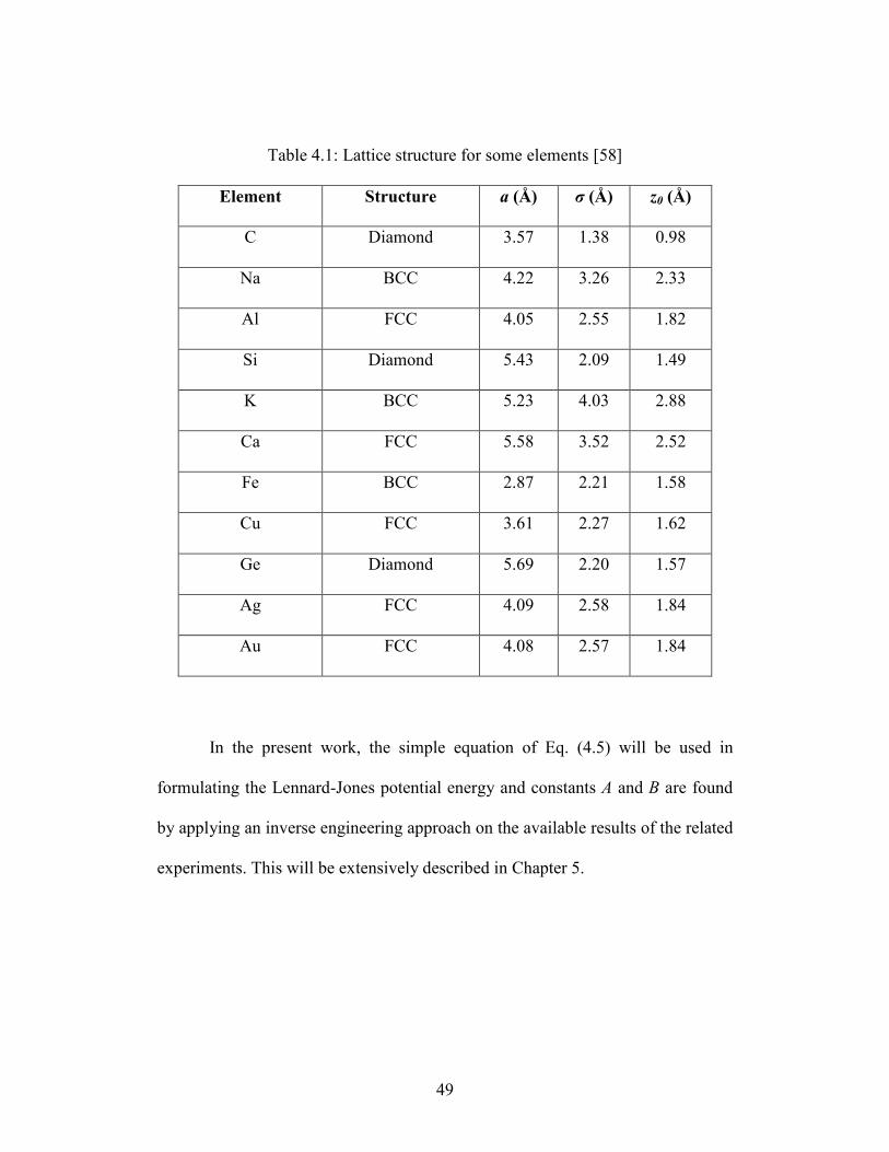
49

Table 4.1: Lattice structure for some elements [58]

Element Structure a (Å) σ (Å) z0 (Å)

C Diamond 3.57 1.38 0.98

Na BCC 4.22 3.26 2.33

Al FCC 4.05 2.55 1.82

Si Diamond 5.43 2.09 1.49

K BCC 5.23 4.03 2.88

Ca FCC 5.58 3.52 2.52

Fe BCC 2.87 2.21 1.58

Cu FCC 3.61 2.27 1.62

Ge Diamond 5.69 2.20 1.57

Ag FCC 4.09 2.58 1.84

Au FCC 4.08 2.57 1.84

In the present work, the simple equation of Eq. (4.5) will be used in

formulating the Lennard-Jones potential energy and constants A and B are found

by applying an inverse engineering approach on the available results of the related

experiments. This will be extensively described in Chapter 5.

50

Electrostatic Forces

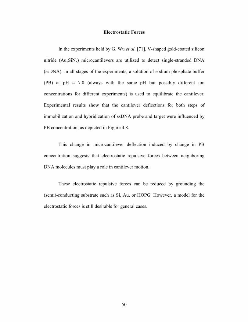
In the experiments held by G. Wu et al. [71], V-shaped gold-coated silicon

nitride (AuySiNx) microcantilevers are utilized to detect single-stranded DNA

(ssDNA). In all stages of the experiments, a solution of sodium phosphate buffer

(PB) at pH ≈ 7.0 (always with the same pH but possibly different ion

concentrations for different experiments) is used to equilibrate the cantilever.

Experimental results show that the cantilever deflections for both steps of

immobilization and hybridization of ssDNA probe and target were influenced by

PB concentration, as depicted in Figure 4.8.

This change in microcantilever deflection induced by change in PB

concentration suggests that electrostatic repulsive forces between neighboring

DNA molecules must play a role in cantilever motion.

These electrostatic repulsive forces can be reduced by grounding the

(semi)-conducting substrate such as Si, Au, or HOPG. However, a model for the

electrostatic forces is still desirable for general cases.

51

Figure 4.8: (a) Steady-state cantilever deflections caused by immobilization of

ssDNA (sequence K-30) at different PB concentrations, (b) Steady-state changes

in cantilever deflection for hybridization of 30-nt-long ssDNA (sequences K-30

and K9-30) at different PB concentrations [71]

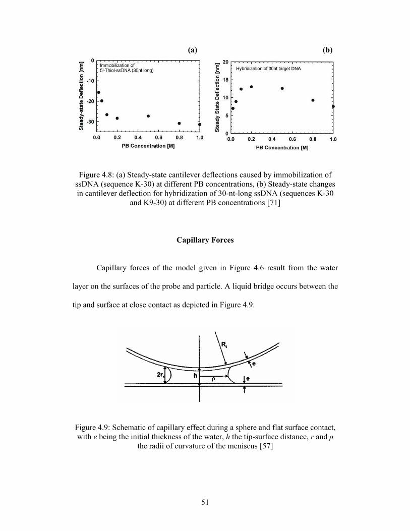
Capillary Forces

Capillary forces of the model given in Figure 4.6 result from the water

layer on the surfaces of the probe and particle. A liquid bridge occurs between the

tip and surface at close contact as depicted in Figure 4.9.

Figure 4.9: Schematic of capillary effect during a sphere and flat surface contact,

with e being the initial thickness of the water, h the tip-surface distance, r and ρ

the radii of curvature of the meniscus [57]

(a) (b)

52

In microcantilever biosensors, we do not have such contact mode as in

AFM applications. Therefore, the capillary effects and forces are neglected in the

microcantilever modeling.

The General Equation of Motion Microcantilever utilizing Hamilton’s Principle

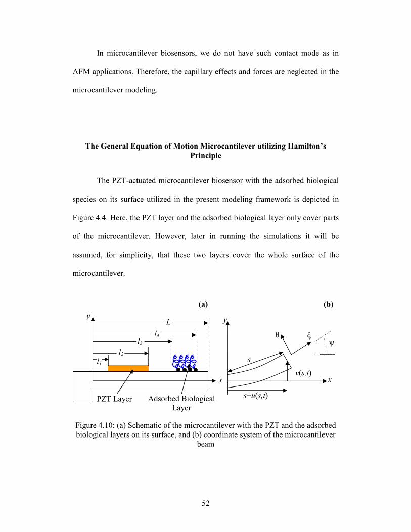
The PZT-actuated microcantilever biosensor with the adsorbed biological

species on its surface utilized in the present modeling framework is depicted in

Figure 4.4. Here, the PZT layer and the adsorbed biological layer only cover parts

of the microcantilever. However, later in running the simulations it will be

assumed, for simplicity, that these two layers cover the whole surface of the

microcantilever.

Figure 4.10: (a) Schematic of the microcantilever with the PZT and the adsorbed

biological layers on its surface, and (b) coordinate system of the microcantilever

beam

v(s,t)

s+u(s,t)

s

x

y

ψ ξ θ

l1

l2

l3 l4

L

x

y

(a) (b)

PZT Layer Adsorbed Biological

Layer

53

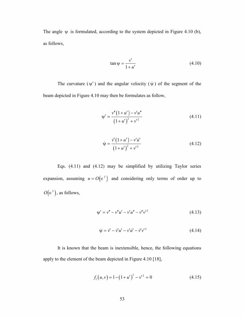
The angle ψ is formulated, according to the system depicted in Figure 4.10 (b),

as follows,

tan1

v

u

′ψ =

′+ (4.10)

The curvature ( ′ψ ) and the angular velocity (ψɺ ) of the segment of the

beam depicted in Figure 4.10 may then be formulates as follow,

( )( )2 2

1

1

v u v u

u v

′′ ′ ′ ′′+ −′ψ =

′ ′+ + (4.11)

( )( )2 2

1

1

v u v u

u v

′ ′ ′ ′+ −ψ =

′ ′+ +

ɺ ɺɺ (4.12)

Eqs. (4.11) and (4.12) may be simplified by utilizing Taylor series

expansion, assuming ( )2u O= ∈ and considering only terms of order up to

( )3O ∈ , as follows,

2v v u v u v v′ ′′ ′′ ′ ′ ′′ ′′ ′ψ = − − − (4.13)

2vvuvuvv ′′−′′−′′−′=ψ ɺɺɺɺɺ (4.14)

It is known that the beam is inextensible, hence, the following equations

apply to the element of the beam depicted in Figure 4.10 [18],

( ) ( )2 2

1 , 1 1 0f u v u v′ ′= − + − = (4.15)

54

Applying Taylor series expansion to Eq. (4.15), u′ and v′ may be related as

follows,

2 211 1

2u v v′ ′ ′= − − ≈ − +⋯ (4.16)

Potential Energy of the Microcantilever Beam

The total kinetic energy of the system depicted in Figure 4.10 (a) is only a

function of the microcantilever structure. The adsorbed biological layer does not

have any effect on the kinetic energy as we have assumed that the effect of

adsorbed mass is negligible compared to that of the induced surface stress.

However, in formulating the total potential energy, the effects of both PZT and

biological layer need to be taken into account. Both kinetic and potential energies

of the microcantilever depicted in Figure 4.10 (a) are derived in the following

sections.

Potential Energy due to the Beam’s Structure Having the PZT Layer on Its Surface

In this section, it is assumed that the PZT layer on the surface of the

microcantilever beam doesn’t store energy. Hence, its effect will be considered in

altering the flexural rigidity of the microcantilever beam only. It is also assumed

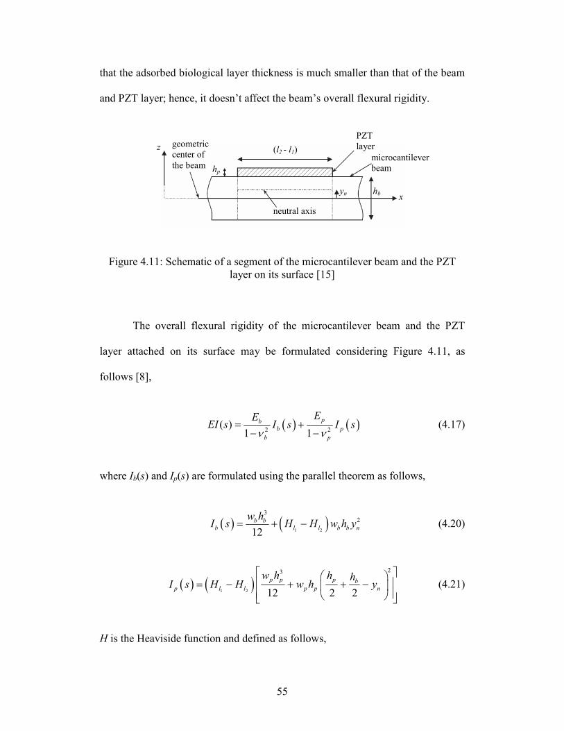
55

that the adsorbed biological layer thickness is much smaller than that of the beam

and PZT layer; hence, it doesn’t affect the beam’s overall flexural rigidity.

Figure 4.11: Schematic of a segment of the microcantilever beam and the PZT

layer on its surface [15]

The overall flexural rigidity of the microcantilever beam and the PZT

layer attached on its surface may be formulated considering Figure 4.11, as

follows [8],

( ) ( )2 2

( )1 1

pb

b p

b p

EEEI s I s I s

ν ν= +

− − (4.17)

where Ib(s) and Ip(s) are formulated using the parallel theorem as follows,

( ) ( )1 2

3

2

12

b b

b l l b b n

w hI s H H w h y= + − (4.20)

( ) ( )1 2

23

12 2 2

p p p b

p l l p p n

w h h hI s H H w h y

= − + + −

(4.21)

H is the Heaviside function and defined as follows,

yn

(l2 - l1)

neutral axis

PZT

layer

microcantilever

beam

hb

hp

geometric

center of

the beam

x

z

56

0 ;

1 ;i

s iH

s i

<=

≥ (4.18)

and yn, is defined as follows,

( )( )bbpp

bppp

nhEhE

hhhEy

+

+=2

(4.19)

Remark: For a microcantilever beam, the thickness of the beam is

typically much smaller than its width and length, thus it is in a “plane strain”

configuration. For this reason, the modulus of elasticity of the microcantilever and

the PZT layer utilized in Eq. (4.17) is corrected from E to 21

E

ν− where ν is the

Poisson’s ratio of the microcantilever or the PZT layer.

Considering terms of order up to ( )4O ∈ , the potential energy due to the

beam’s structure and the attached PZT layer may be formulated as follows,

( ) ( )( )2 2 2 2 2

0 0

1 12 2 2

2 2

L L

bpU EI s ds EI s v v v v u v v u dsψ ′ ′′ ′′ ′ ′′ ′ ′ ′′ ′′= = − − −∫ ∫ (4.22)

Potential Energy due to the Energy Storage of the PZT Layer

The potential energy may be found using the following equation [40],

0

1

2

L

cU M dsψ ′= ∫ (4.23)

57

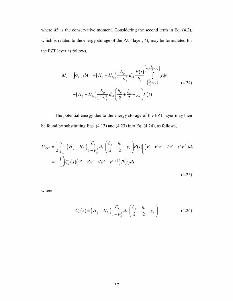
where Mc is the conservative moment. Considering the second term in Eq. (4.2),

which is related to the energy storage of the PZT layer, Mc may be formulated for

the PZT layer as follows,

( ) ( )

( ) ( )

1 2

1 2

2

11 312

2

312

1

2 21

bp n

bn

hh y

p

c l l

p hpy

p p b

l l n

p

E P tM ydA H H d ydy

h

E h hH H d y P t

+ −

−

= σ = − −− ν

= − − + −

− ν

∫ ∫ (4.24)

The potential energy due to the energy storage of the PZT layer may then

be found by substituting Eqs. (4.13) and (4.23) into Eq. (4.24), as follows,

( ) ( ) ( )

( )( ) ( )

1 2

2

312

0

2

0

1

2 2 21

1

2

Lp p b

PZT l l n

p

L

c

E h hU H H d y P t v v u v u v v ds

C s v v u v u v v P t ds

ν

′′ ′′ ′ ′ ′′ ′′ ′= − − + − − − −

−

′′ ′′ ′ ′ ′′ ′′ ′= − − − −

∫

∫

(4.25)

where

( ) ( )1 2 312 2 21

p p b

c l l n

p

E h hC s H H d y

ν

= − + −

− (4.26)

58

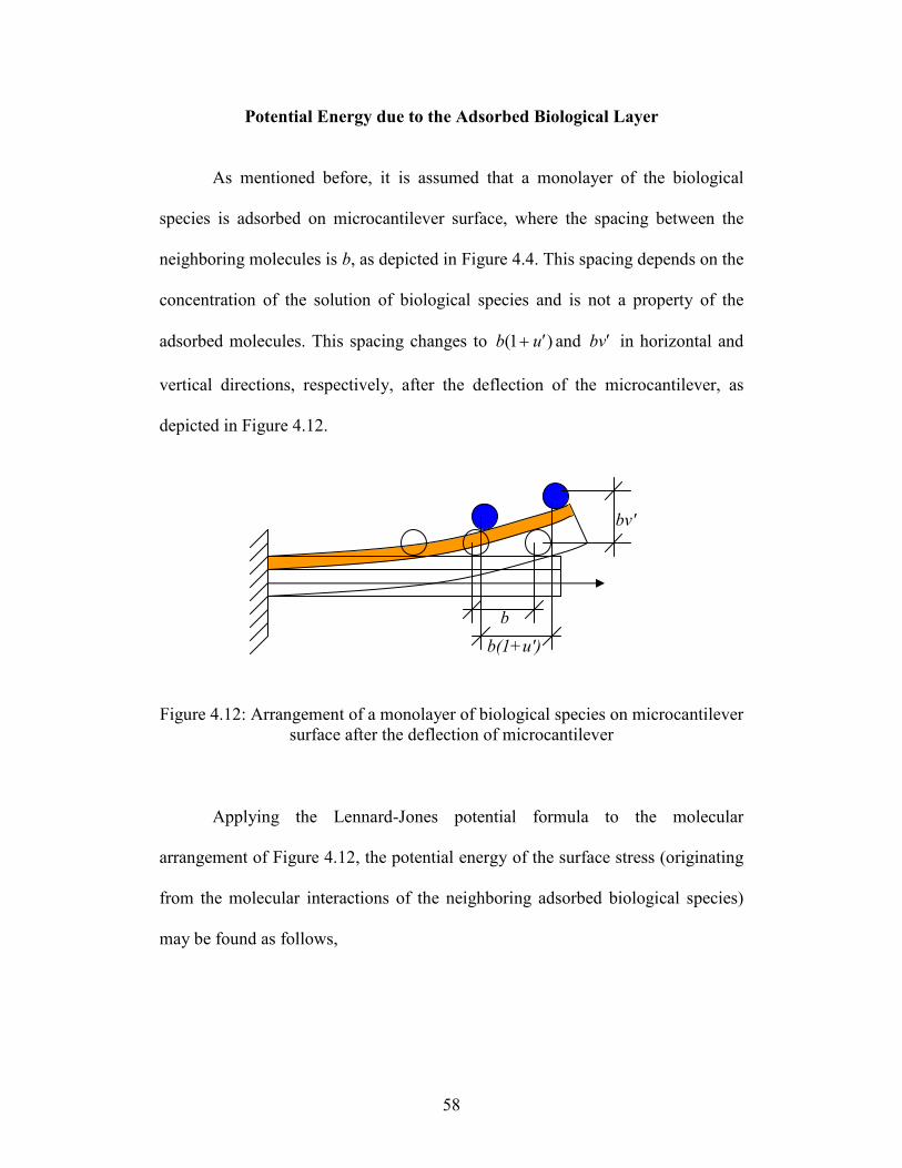
Potential Energy due to the Adsorbed Biological Layer

As mentioned before, it is assumed that a monolayer of the biological

species is adsorbed on microcantilever surface, where the spacing between the

neighboring molecules is b, as depicted in Figure 4.4. This spacing depends on the

concentration of the solution of biological species and is not a property of the

adsorbed molecules. This spacing changes to (1 )b u′+ and bv′ in horizontal and

vertical directions, respectively, after the deflection of the microcantilever, as

depicted in Figure 4.12.

Figure 4.12: Arrangement of a monolayer of biological species on microcantilever

surface after the deflection of microcantilever

Applying the Lennard-Jones potential formula to the molecular

arrangement of Figure 4.12, the potential energy of the surface stress (originating

from the molecular interactions of the neighboring adsorbed biological species)

may be found as follows,

b(1+u′)

b

bv′

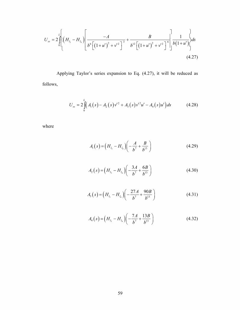
59

( )( ) ( ) ( )3 4 3 6

2 26 2 12 20

12

11 1

L

ss l l

A BU H H ds

b ub u v b u v

−

= − + ′+ ′ ′ ′ ′+ + + +

∫

(4.27)

Applying Taylor’s series expansion to Eq. (4.27), it will be reduced as

follows,

( ) ( ) ( ) ( )( )2 2

1 2 3 4

0

2

L

ssU A s A s v A s v u A s u ds′ ′ ′ ′= − + −∫ (4.28)

where

( ) ( )3 41 7 13l l

A BA s H H

b b

= − − +

(4.29)

( ) ( )3 42 7 13

3 6l l

A BA s H H

b b

= − − +

(4.30)

( ) ( )3 43 7 13

27 90l l

A BA s H H

b b

= − − +

(4.31)

( ) ( )3 44 7 13

7 13l l

A BA s H H

b b

= − − +

(4.32)

60

Total Potential Energy of the Microcantilever Beam with the PZT Layer and the Adsorbed Biological Layer

Putting Eqs. (4.22), (4.25) and (4.28) together, total potential energy of the

system can be formulated as follows,

( )( ){( )( ) ( )

( ) ( ) ( ) ( ) }

2 2 2 2

0

2

2 2

1 2 3 4

12 2 2

2

4

L

bp PZT ss

c

U U U U EI s v v v v u v v u

C s v v u v u v v P t

A s A s v A s v u A s u ds

′′ ′′ ′ ′′ ′ ′ ′′ ′′= + + = − − −

′′ ′′ ′ ′ ′′ ′′ ′− − − −

′ ′ ′ ′ + − + −

∫

(4.33)

Kinetic Energy of the Microcantilever Beam

The total kinetic energy of the microcantilever beam and the PZT layer

and adsorbed biological layer, as depicted in Figure 4.10 (a), may be formulated

as follows,

( ) ( )2 2

0

1

2

L

m s u v dsT + = ∫ ɺ ɺ (4.34)

where

( )1 2

( ) p pb b b l lm s w h H H h

= ρ + − ρ (4.35)

It is assumed that the mass of the adsorbed biological layer is negligible.

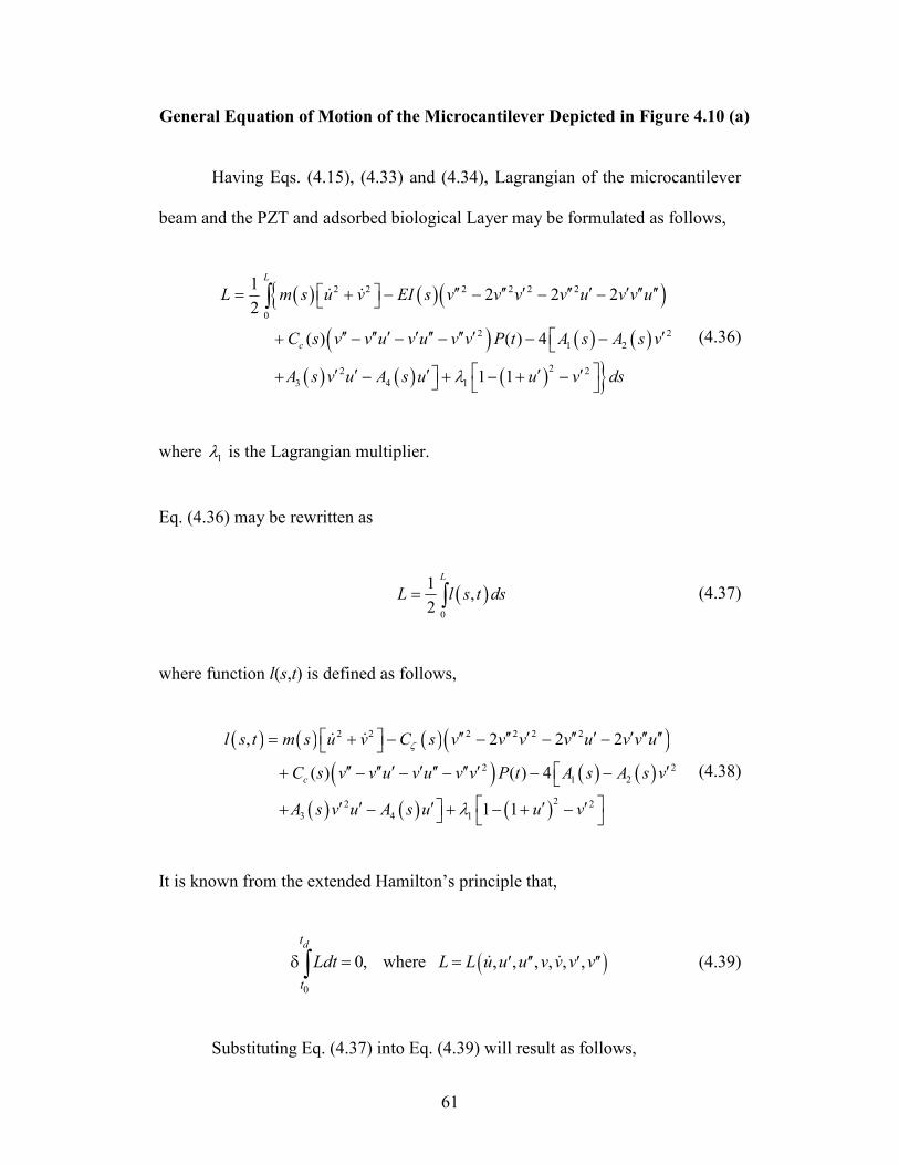
61

General Equation of Motion of the Microcantilever Depicted in Figure 4.10 (a)

Having Eqs. (4.15), (4.33) and (4.34), Lagrangian of the microcantilever

beam and the PZT and adsorbed biological Layer may be formulated as follows,

( ) ( )( ){( ) ( ) ( )

( ) ( ) ( ) }

2 2 2 2 2 2

0

2 2

1 2

22 2

3 4 1

12 2 2

2

( ) ( ) 4

1 1

L

c

L m s u v EI s v v v v u v v u

C s v v u v u v v P t A s A s v

A s v u A s u u v dsλ

′′ ′′ ′ ′′ ′ ′ ′′ ′′ = + − − − −

′′ ′′ ′ ′ ′′ ′′ ′ ′+ − − − − −

′ ′ ′ ′ ′+ − + − + −

∫ ɺ ɺ

(4.36)

where 1λ is the Lagrangian multiplier.

Eq. (4.36) may be rewritten as

( )0

1,

2

L

L l s t ds= ∫ (4.37)

where function l(s,t) is defined as follows,

( ) ( ) ( )( )( ) ( ) ( )

( ) ( ) ( )

2 2 2 2 2 2

2 2

1 2

22 2

3 4 1

, 2 2 2

( ) ( ) 4

1 1

c

l s t m s u v C s v v v v u v v u

C s v v u v u v v P t A s A s v

A s v u A s u u v

ζ

λ

′′ ′′ ′ ′′ ′ ′ ′′ ′′ = + − − − −

′′ ′′ ′ ′ ′′ ′′ ′ ′+ − − − − −

′ ′ ′ ′ ′+ − + − + −

ɺ ɺ

(4.38)

It is known from the extended Hamilton’s principle that,

( )0

0, where , , , , , ,dt

t

Ldt L L u u u v v v vδ = = ′ ′′ ′ ′′∫ ɺ ɺ (4.39)

Substituting Eq. (4.37) into Eq. (4.39) will result as follows,

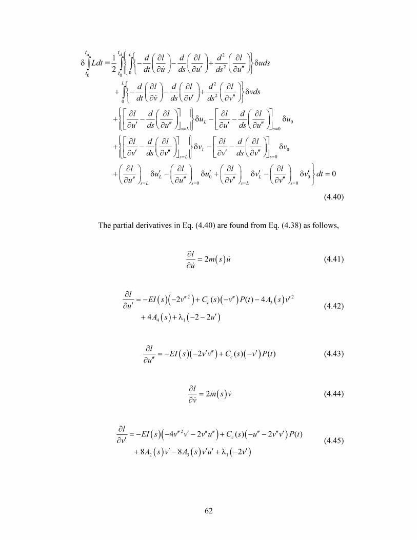
62

2

2

00 0

2

2

0

1

2

d d L

L

L

s L

t t

t t

d l d l d lLdt uds

dt u ds u uds

d l d l d lvds

dt v ds v vds

l d l l du

u ds u u ds=

∂ ∂ ∂ δ − − + δ ′ ′′∂ ∂ ∂

∂ ∂ ∂ + − − + δ ′ ′′∂ ∂ ∂

∂ ∂ ∂ ∂ + − δ − − ′ ′′ ′∂ ∂ ∂

= ∫

∫

∫ ∫ ɺ

ɺ

0

0

0

0

0 0

0 0

0

s

L

s L s

L L

s L s s L s

lu

u

l d l l d lv v

v ds v v ds v

l l l lu u v v dt

u u v v

=

= =

= = = =

δ ′′∂

∂ ∂ ∂ ∂ + − δ − − δ ′ ′′ ′ ′′∂ ∂ ∂ ∂

∂ ∂ ∂ ∂ ′ ′ ′ ′+ δ − δ + δ − δ = ′′ ′′ ′′ ′′∂ ∂ ∂ ∂

(4.40)

The partial derivatives in Eq. (4.40) are found from Eq. (4.38) as follows,

( )2l

m s uu

∂=

∂ɺ

ɺ (4.41)

( )( ) ( ) ( )

( ) ( )

2 2

3

4 1

2 ( ) ( ) 4

4 2 2

c

lEI s v C s v P t A s v

u

A s u

∂ ′′ ′′ ′= − − + − −′∂

′+ + λ − − (4.42)

( )( ) ( )2 ( ) ( )c

lEI s v v C s v P t

u

∂ ′ ′′ ′= − − + −′′∂

(4.43)

( )2l

m s vv

∂=

∂ɺ

ɺ (4.44)

( ) ( ) ( )

( ) ( ) ( )

2

2 3 1

4 2 ( ) 2 ( )

8 8 2

c

lEI s v v v u C s u v v P t

v

A s v A s v u v

∂ ′′ ′ ′′ ′′ ′′ ′′ ′= − − − + − −′∂

′ ′ ′ ′+ − + λ − (4.45)

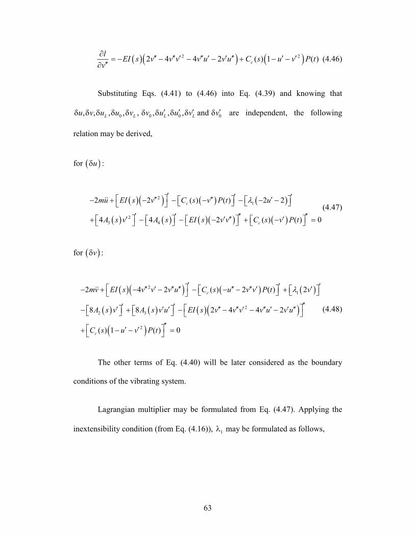
63

( )( ) ( )2 22 4 4 2 ( ) 1 ( )c

lEI s v v v v u v u C s u v P t

v

∂ ′′ ′′ ′ ′′ ′ ′ ′′ ′ ′= − − − − + − −′′∂

(4.46)

Substituting Eqs. (4.41) to (4.46) into Eq. (4.39) and knowing that

0, , , , ,L Lu v u u vδ δ δ δ δ 0 0 0, , , andL Lv u u v v′ ′ ′ ′δ δ δ δ δ are independent, the following

relation may be derived,

for ( )uδ :

( )( ) ( ) ( )

( ) ( ) ( )( ) ( )

2

1

2

3 4

2 2 ( ) ( ) 2 2

4 4 2 ( ) ( ) 0

c

c

mu EI s v C s v P t u

A s v A s EI s v v C s v P t

λ′ ′ ′ ′′ ′′ ′ − + − − − − − −

′ ′ ′′ ′′′ ′ ′′ ′ + − − − + − =

ɺɺ(4.47)

for ( )vδ :

( )( ) ( ) ( )

( ) ( ) ( )( )

( )

2

1

2

2 3

2

2 4 2 ( ) 2 ( ) 2

8 8 2 4 4 2

( ) 1 ( ) 0

c

c

mv EI s v v v u C s u v v P t v

A s v A s v u EI s v v v v u v u

C s u v P t

λ′ ′ ′ ′′ ′ ′′ ′′ ′′ ′′ ′ ′ − + − − − − − +

′′′ ′ ′ ′ ′ ′′ ′′ ′ ′′ ′ ′ ′′ − + − − − −

′′ ′ ′+ − − =

ɺɺ

(4.48)

The other terms of Eq. (4.40) will be later considered as the boundary

conditions of the vibrating system.

Lagrangian multiplier may be formulated from Eq. (4.47). Applying the

inextensibility condition (from Eq. (4.16)), 1λ may be formulated as follows,

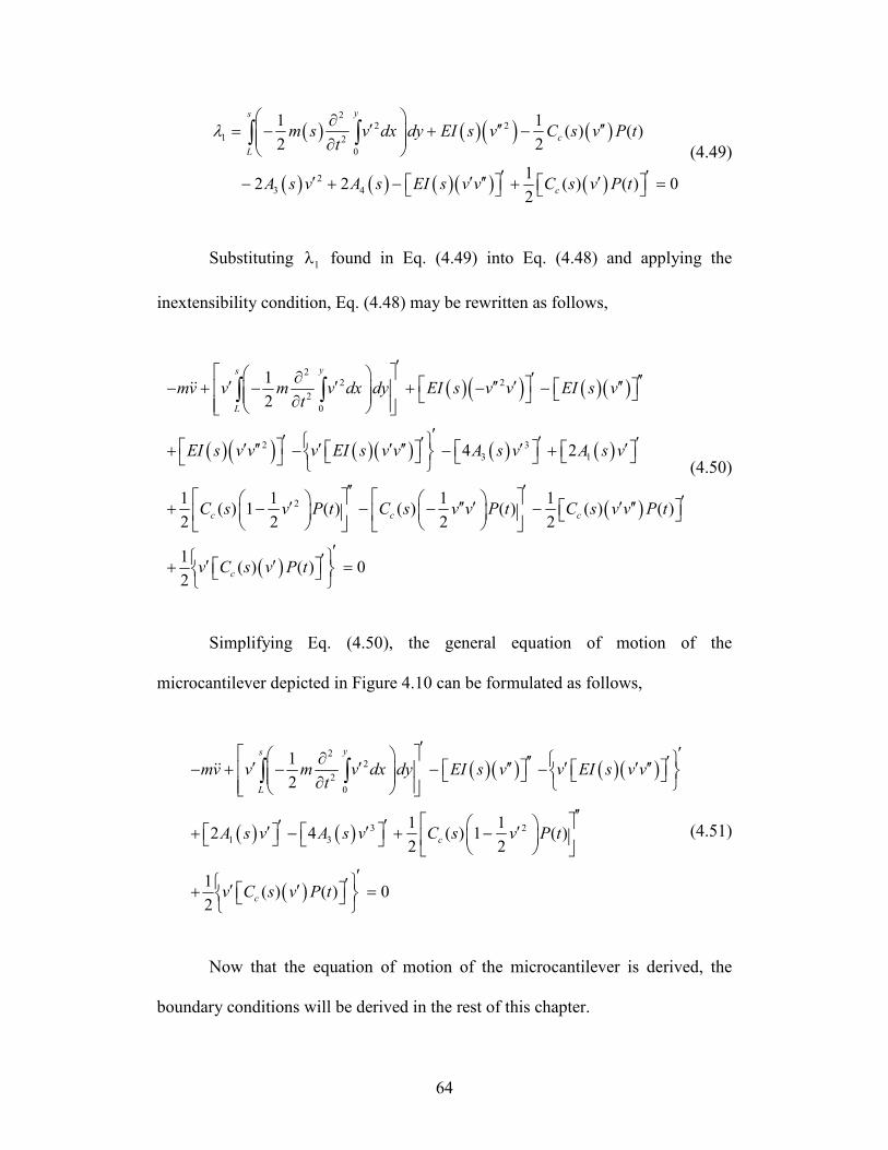
64

( ) ( )( ) ( )

( ) ( ) ( )( ) ( )

22 2

1 2

0

2

3 4

1 1( ) ( )

2 2

12 2 ( ) ( ) 0

2

ys

c

L

c

m s v dx dy EI s v C s v P tt

A s v A s EI s v v C s v P t

λ ∂

′ ′′ ′′= − + − ∂

′ ′′ ′ ′′ ′ − + − + =

∫ ∫ (4.49)

Substituting 1λ found in Eq. (4.49) into Eq. (4.48) and applying the

inextensibility condition, Eq. (4.48) may be rewritten as follows,

( )( ) ( )( )

( )( ) ( )( ) ( ) ( )

22 2

2

0

2 3

3 1

2

1

2

4 2

1 1 1( ) 1 ( ) ( ) ( )

2 2 2

ys

L

c c

mv v m v dx dy EI s v v EI s vt

EI s v v v EI s v v A s v A s v

C s v P t C s v v P t

′ ∂ ′ ′′ ′ ′ ′′ ′ ′′ − + − + − − ∂

′′ ′′ ′ ′ ′′ ′ ′ ′′ ′ ′ + − − +

′′ ′ ′′ ′+ − − −

∫ ∫ɺɺ

( )

( )

1( ) ( )

2

1( ) ( ) 0

2

c

c

C s v v P t

v C s v P t

′′′ ′′ −

′ ′′ ′ + =

(4.50)

Simplifying Eq. (4.50), the general equation of motion of the

microcantilever depicted in Figure 4.10 can be formulated as follows,

( )( ) ( )( )

( ) ( )

( )

22

2

0

3 2

1 3

1

2

1 12 4 ( ) 1 ( )

2 2

1( ) ( ) 0

2

ys

L

c

c

mv v m v dx dy EI s v v EI s v vt

A s v A s v C s v P t

v C s v P t

′ ′ ∂ ′′ ′′ ′ ′′ ′ ′ ′′ − + − − − ∂

′′ ′′′ ′ ′ + − + −

′ ′′ ′ + =

∫ ∫ɺɺ

(4.51)

Now that the equation of motion of the microcantilever is derived, the

boundary conditions will be derived in the rest of this chapter.

65

The geometric admissibility results in the following relation,

(0, ) 0v t = (4.52)

which may be rewritten as follows,

0 0vδ = (4.53)

Equations giving the boundary conditions are derived from Eq. (4.40) as

follows,

for ( )Lv′δ :

0l

s l

lv

v =

∂ ′δ = ′′∂ (4.54)

Substituting Eq. (4.46) into Eq. (4.54) will result in the following relation,

( )( )2 212 ( ) 1 ( ) 0

2L c L LEI L v C L v P t vδ

′′ ′ ′− + − =

(4.55)

Lv′δ being arbitrary, Eq. (4.55) will result in the following relation,

( )( )2 212 ( ) 1 ( ) 0

2L c LEI L v C L v P t

′′ ′− + − =

(4.56)

It is derived from Eq. (4.26) that ( ) 0cC L = . Even if the piezoelectric layer

covers the whole length of the microcantilever, it is a correct assumption to

consider 2L l− = ε . Thus, Eq. (4.56) reduces to the following equation,

66

( )( )22 0LEI L v′′− = (4.57)

Knowing that ( ) 0EI L ≠ the following relation may be concluded,

0Lv′′ = (4.58)

for ( )Lvδ :

1 10

2 2L

s L

l d lv

v ds v =

∂ ∂ − δ = ′ ′′∂ ∂ (4.59)

Substituting Eqs. (4.25) and (4.46) into Eq. (4.59) the following equation

may be formulated,

( )( ) ( ) ( ){

( )( )

2

1

2

2 ( ) ( ) 2

12 ( ) 1 ( ) 0

2

L L c L L L

c Ls Ls L

EI L v v C L v v P t v

EI s v C s v P t v=

=

′′ ′ ′′ ′ ′− − + − + λ −

′ ′′′ ′ − − + − δ =

(4.60)

Lvδ being arbitrary, Eq. (4.60) will result in the following relation,

( )( ) ( ) ( )

( )( )

2

1

2

2 ( ) ( ) 2

12 ( ) 1 ( ) 0

2

L L c L L L

cs Ls L

EI L v v C L v v P t v

EI s v C s v P t=

=

′′ ′ ′′ ′ ′− − + − + λ −

′ ′′′ ′ − − + − =

(4.61)

Assuming ( )EI s′ and ( )cC s′ are zero and considering Eq. (4.58), Eq.

(4.61) will be rewritten as follows,

67

( ) ( )2 1 0L LEI L v v′′′ ′ + = (4.62)

Therefore, the second boundary condition at s=L will be found from Eq.

(4.62) as follows,

0Lv′′′= (4.63)

for ( )0vδ :

0

0

1 10

2 2s

l d lv

v ds v =

∂ ∂ − δ = ′ ′′∂ ∂ (4.64)

Having 0 0vδ = from Eq. (4.53), Eq. (4.64) doesn’t result in a new

boundary condition.

for ( )0v′δ :

0

0

0s

lv

v =

∂ ′δ = ′′∂ (4.65)

Substituting Eq. (4.46) into Eq. (4.65) will result in the following relation,

( )( )2 2

0 0 0

10 2 (0) 1 ( ) 0

2cEI v C v P t vδ

′′ ′ ′− + − =

(4.66)

Assuming 0v′δ is arbitrary, Eq. (4.66) will give the following equation,

68

( )( )2 2

0 0

10 2 (0) 1 ( ) 0

2cEI v C v P t

′′ ′− + − =

(4.67)

It is derived from Eq. (4.26) that (0) 0cC = . Even if the piezoelectric layer

covers the whole length of the microcantilever, it is a correct assumption to

consider 1l = ε . Thus, Eq. (4.67) reduces to the following,

( )( )200 2 0EI v′′− = (4.68)

However, it is concluded from Eq. (4.17) that ( )0 0EI ≠ and also due to

the nonzero moment at s=0, 0 0v′′ ≠ . This means that Eq. (4.67) may not be

satisfied unless 0v′δ equals zero,

0 00 0v v′ ′δ = ⇒ = (4.69)

Thus, the general equation of motion and the boundary conditions of the

vibrating microcantilever beam depicted in Figure 4.10 will be as follows,

( )( ) ( )( )

( ) ( )

( )

22

2

0

3 2

1 3

1

2

1 12 4 ( ) 1 ( )

2 2

1( ) ( ) 0

2

ys

L

c

c

mv v m v dx dy EI s v v EI s v vt

A s v A s v C s v P t

v C s v P t

′ ′ ∂ ′′ ′′ ′ ′′ ′ ′ ′′ − + − − − ∂

′′ ′′′ ′ ′ + − + −

′ ′′ ′ + =

∫ ∫ɺɺ

(4.70)

69

At s=0:

0v v′= = (4.71)

At s=L:

0v v′′ ′′′= = (4.72)

70

CHAPTER 5

SOLUTION TO THE NONLINEAR EQUATIONS OF MOTION OF THE

MICROCANTILEVER

The nonlinear equation of motion of the piezoelectrically-driven

microcantilever beam with a layer of the adsorbed biological species, depicted

schematically in Figure 4.10 (a), was derived in the previous chapter, Eq. (4.70),

with the boundary conditions of Eqs. (4.71) and (4.72).

The beam deflection, ( , )v s t , can be truncated into n-modes as follows,

1 1

( , ) ( , ) ( ) ( )n n

i i i

i i

v s t v s t s q t= =

= = φ∑ ∑ (5.1)

where φi is the comparison function (satisfying only the boundary conditions and

not necessarily the equations of motion) and qi is the generalized time-dependent

coordinate for ith mode of the beam. For the cantilever boundary conditions

considered in Eqs. (4.71) and (4.72), the following linear mode shapes of bending

are considered

72

cosh( ) cos( )( ) cosh( ) cos( ) [sin( ) sinh( )]

sin( ) sinh( )

i i

i i i i i i

i i

L Ls A s s s s

L L

λ + λφ = λ − λ + λ − λ

λ + λ (5.2)

where λi are the roots of the following frequency equation,

1 cos( )cosh( ) 0i iL L+ λ λ = (5.3)

and Ai is a constant being obtained using the orthogonality condition (of the mode

shapes).

Substituting Eqs. (5.1) and (5.2) into Eq. (4.70) and taking the inner

product of the resulting equation with φi(s) yields the following ordinary

differential equation for qi(t)

( )3 2 2 2

1 2 3 4 5 6( ) ( )i i i i i i i i i i i i i ig q g q g q g q q q q g q P t g P t+ + + + − =ɺɺ ɺɺ ɺ (5.4)

where

2

1

0

( ) ( )

L

i ig m s s ds= φ∫ (5.5)

( ) ( )( )2 1

0

( ) ( ) ( ) 2 ( )

L

i i i ig s EI s s A s s ds′″ ′′ ′= φ φ − φ ∫ (5.6)

( ) ( )

( )

2 2

3

0

3

3

( ) ( ) ( ) ( ) ( ) ( ) ( ) ( )

4 ( ) ( ) ( )

L

i i i i i i i

i i

g s EI s s s s EI s s s

s A s s ds

′ ″ ′ ′′ ′ ′′= φ φ φ + φ φ φ′ ′+ φ φ

∫ (5.7)

73

2

4

0 0

( ) ( ) 2 ( )

yL s

i i i i

L

g m s s x dxdy ds

′ ′ ′= φ φ φ

∫ ∫ ∫ (5.8)

( ) ( )2

5

0 0

1( ) ( ) ( ) ( ) ( ) ( ) ( )

2

L L

i i c i i i c ig s C s s s ds s C s s ds″′′ ′′ ′= φ φ φ + φ φ∫ ∫ (5.9)

6

0

1( ) ( )

2

L

i i cg s C s ds′′= φ∫ (5.10)

Using Eq. (5.4), the nonlinear equation of motion of the microcantilever

given in Eq. (4.70) can be simulated using Matlab/Simulink

. The Matlab code

and simulation diagrams are both given in Appendix A. Results and discussions

of the simulation are discussed in the following sections.

Numerical Simulations and Results

Considering the general equation of motion of the microcantilever given in

Eq. (4.70) or its discretized version given by Eq. (5.4), the resonance frequency of

the PZT-driven microcantilever with the adsorbed biological species can be

found. In order to run the simulation for deriving the solution to Eq. (5.4),

structural properties of the microcantilever beam and the attached PZT layer

together with Lennard-Jones constants and molecular spacing of the adsorbed

biological species are needed. The microcantilever and the PZT layer considered

here and in the simulations have the following properties,

74

3

Beam: (length) 500 µm

(width) 100 µm

(thickness) 1µm

0 23

170GPa

2330 kg/m

L

w

t

ν .

E

ρ

==

===

=

3

PZTLayer: (length) 500 µm

(width) 100 µm

(thickness) 0.5µm

0 25

133GPa

6390 kg/m

L

w

t

ν .

E

ρ

==

===

≅

(5.11)

The Lennard-Jones constants and molecular spacing of the biological

species are also needed. As mentioned earlier, it is not easy to find the Lennard-

Jones constants of biological species. The Lennard-Jones constants for different

molecular structures vary in the range of A=2×10-79 to 1×10-76 J.m6 and B=2×10-

136 to 4×10-134 J.m12

[11, 71]. There exist different tables of the Lennard-Jones

constants for gases, however, these constants are found empirically for each

biological species in the desired conditions.

In our modeling, in order to have an estimate of these Lennard-Jones

constants and due to the fact that were no in-house experimental results available,

the McFarland et al.’s results [42] were utilized and the inverse engineering was

performed. This is done in order to obtain the resonance frequency shifts as

measured in McFarland et al. experiment. Hence, the following physical

properties of microcantilever beam are considered here.

3

(length) 500µm

(width) 100 µm

(thickness) 1µm

0 23

170GPa

2330 kg/m

b

L

w

t

ν .

E

ρ

==

===

=

(5.12)

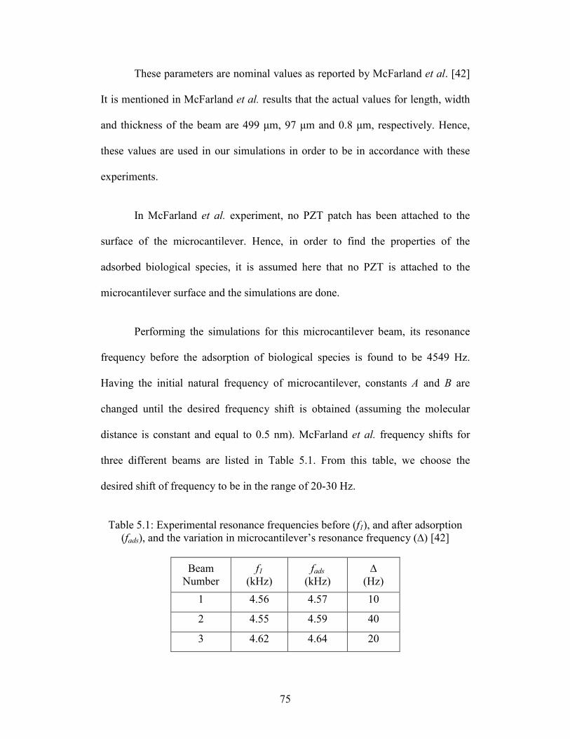
75

These parameters are nominal values as reported by McFarland et al. [42]

It is mentioned in McFarland et al. results that the actual values for length, width

and thickness of the beam are 499 µm, 97 µm and 0.8 µm, respectively. Hence,

these values are used in our simulations in order to be in accordance with these

experiments.

In McFarland et al. experiment, no PZT patch has been attached to the

surface of the microcantilever. Hence, in order to find the properties of the

adsorbed biological species, it is assumed here that no PZT is attached to the

microcantilever surface and the simulations are done.

Performing the simulations for this microcantilever beam, its resonance

frequency before the adsorption of biological species is found to be 4549 Hz.

Having the initial natural frequency of microcantilever, constants A and B are

changed until the desired frequency shift is obtained (assuming the molecular

distance is constant and equal to 0.5 nm). McFarland et al. frequency shifts for

three different beams are listed in Table 5.1. From this table, we choose the

desired shift of frequency to be in the range of 20-30 Hz.

Table 5.1: Experimental resonance frequencies before (f1), and after adsorption

(fads), and the variation in microcantilever’s resonance frequency (∆) [42]

Beam

Number

f1 (kHz)

fads

(kHz)

∆

(Hz)

1 4.56 4.57 10

2 4.55 4.59 40

3 4.62 4.64 20

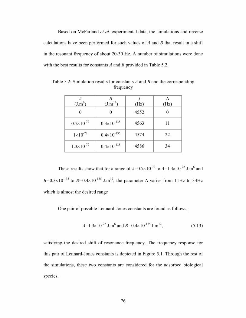
76

Based on McFarland et al. experimental data, the simulations and reverse

calculations have been performed for such values of A and B that result in a shift

in the resonant frequency of about 20-30 Hz. A number of simulations were done

with the best results for constants A and B provided in Table 5.2.

Table 5.2: Simulation results for constants A and B and the corresponding

frequency

A

(J.m6)

B

(J.m12)

f

(Hz)

∆

(Hz)

0 0 4552 0

0.7×10-72 0.3×10-135 4563 11

1×10-72 0.4×10-135 4574 22

1.3×10-72 0.4×10-135 4586 34

These results show that for a range of A=0.7×10-72 to A=1.3×10-72 J.m6 and

B=0.3×10-135 to B=0.4×10-135 J.m12, the parameter ∆ varies from 11Hz to 34Hz

which is almost the desired range

One pair of possible Lennard-Jones constants are found as follows,

A=1.3×10-72 J.m6 and B=0.4×10-135 J.m12

, (5.13)

satisfying the desired shift of resonance frequency. The frequency response for

this pair of Lennard-Jones constants is depicted in Figure 5.1. Through the rest of

the simulations, these two constants are considered for the adsorbed biological

species.

77

Figure 5.1: Frequency response of a microcantilever with properties listed in Eq.

(5.12) and the adsorbed biological species on its surface having Lennard-Jones

constants of A=1.3×10-72 J.m6 and B=0.4×10-135 J.m12

The obtained constants A and B, however, do not match the typical range

for molecules (and biological species). It should be mentioned that the

intermolecular forces of attraction/repulsion are not the only adhesion forces

present. Our results clearly show that other adhesion forces such as electrostatic

interactions have non-negligible effects on the resonance response of the system.

It is also demonstrated that there exist other sources accounting for the surface

stress such as the surface charge redistribution of the underlying substrate. This

may have a dominant role in the resonance frequency shift of the microcantilever

[42]. It is important to mention that these effects are even more dominant than the

attraction/repulsion effect, since the Lennard-Jones constants found here are far

beyond the reality. Therefore, the obtained constants need to be refurbished by

considering the mentioned forces and effects in further investigations.

0 1000 2000 3000 4000 5000 6000 7000 8000 Frequency (Hz)

v(L, t) (Micrometer)

Response

f=4525 Hz

Excitation f=4549 Hz

5

4.5

4 3.5

3 2.5

2

1.5 1

0.5

0

78

Remark: The value of b as mentioned in Chapter 4 depends on the

concentration of the solution. We assume this parameter to be 0.5 nm and will

later (in the following sections) study how it is related to the resonance frequency

of microcantilever beam.

As mentioned earlier in this section, the resonance frequency of the

vibrating microcantilever may be numerically derived from Eq. (5.4). In the

following sections, the effects of the adsorbed biological and the attached PZT

layers on the resonance frequency of microcantilever beam are investigated. The

nonlinear terms and their influence on the frequency response of the system are

first studied for the case where there is no biological layer adsorbed on the surface

of the microcantilever (before the adsorption); hence, only the effect of the

attached PZT layer is investigated. Having the effect of PZT layer on the shift in

the frequency studied, it is assumed that the biological layer is adsorbed and the

effect of both layers is investigated on the shift in the resonance frequency of the

vibrating microcantilever.

The Effect of the Attached PZT Layer

Unlike the biological layer with its thickness and rigidity being negligible,

the attached PZT layer is thick enough to change the rigidity of the system.

Considering the microcantilever studied before, a PZT layer with the properties

listed in Eq. (5.11) is considered to be attached on its surface.

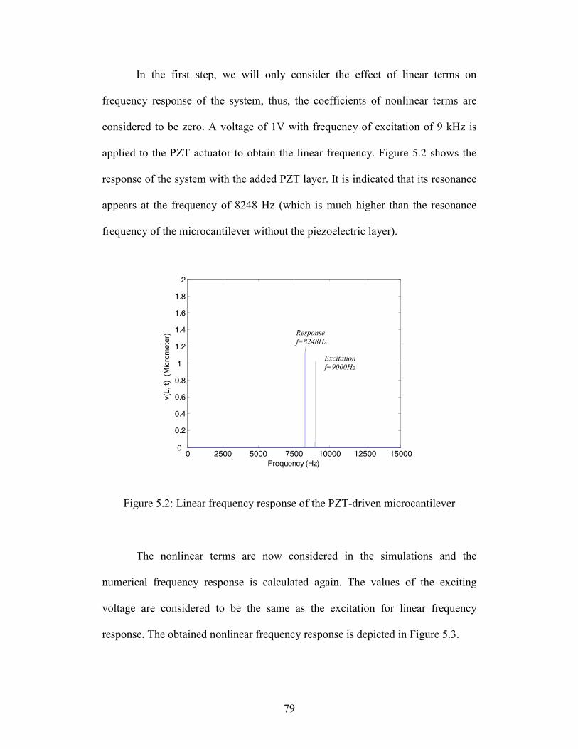
79

In the first step, we will only consider the effect of linear terms on

frequency response of the system, thus, the coefficients of nonlinear terms are

considered to be zero. A voltage of 1V with frequency of excitation of 9 kHz is

applied to the PZT actuator to obtain the linear frequency. Figure 5.2 shows the

response of the system with the added PZT layer. It is indicated that its resonance

appears at the frequency of 8248 Hz (which is much higher than the resonance

frequency of the microcantilever without the piezoelectric layer).

0 2500 5000 7500 10000 12500 150000

0.2

0.4

0.6

0.8

1

1.2

1.4

1.6

1.8

2

Frequency (Hz)

v(l,t)

(Mic

rom

ete

r)

Figure 5.2: Linear frequency response of the PZT-driven microcantilever

The nonlinear terms are now considered in the simulations and the

numerical frequency response is calculated again. The values of the exciting

voltage are considered to be the same as the excitation for linear frequency

response. The obtained nonlinear frequency response is depicted in Figure 5.3.

Excitation

f=9000Hz

Response

f=8248Hz

v(L, t) (Micrometer)

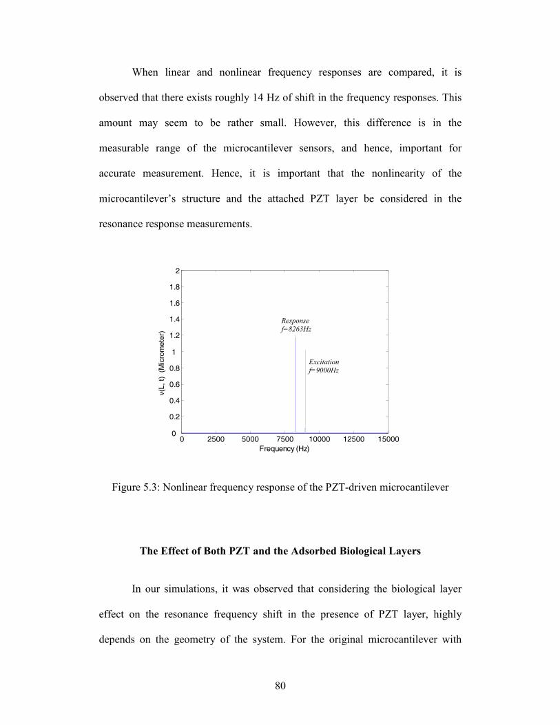
80

When linear and nonlinear frequency responses are compared, it is

observed that there exists roughly 14 Hz of shift in the frequency responses. This

amount may seem to be rather small. However, this difference is in the

measurable range of the microcantilever sensors, and hence, important for

accurate measurement. Hence, it is important that the nonlinearity of the

microcantilever’s structure and the attached PZT layer be considered in the

resonance response measurements.

0 2500 5000 7500 10000 12500 150000

0.2

0.4

0.6

0.8

1

1.2

1.4

1.6

1.8

2

Frequency (Hz)

v(l,t)

(Mic

rom

ete

r)

Figure 5.3: Nonlinear frequency response of the PZT-driven microcantilever

The Effect of Both PZT and the Adsorbed Biological Layers

In our simulations, it was observed that considering the biological layer

effect on the resonance frequency shift in the presence of PZT layer, highly

depends on the geometry of the system. For the original microcantilever with

Response f=8263Hz

Excitation f=9000Hz

v(L, t) (Micrometer)

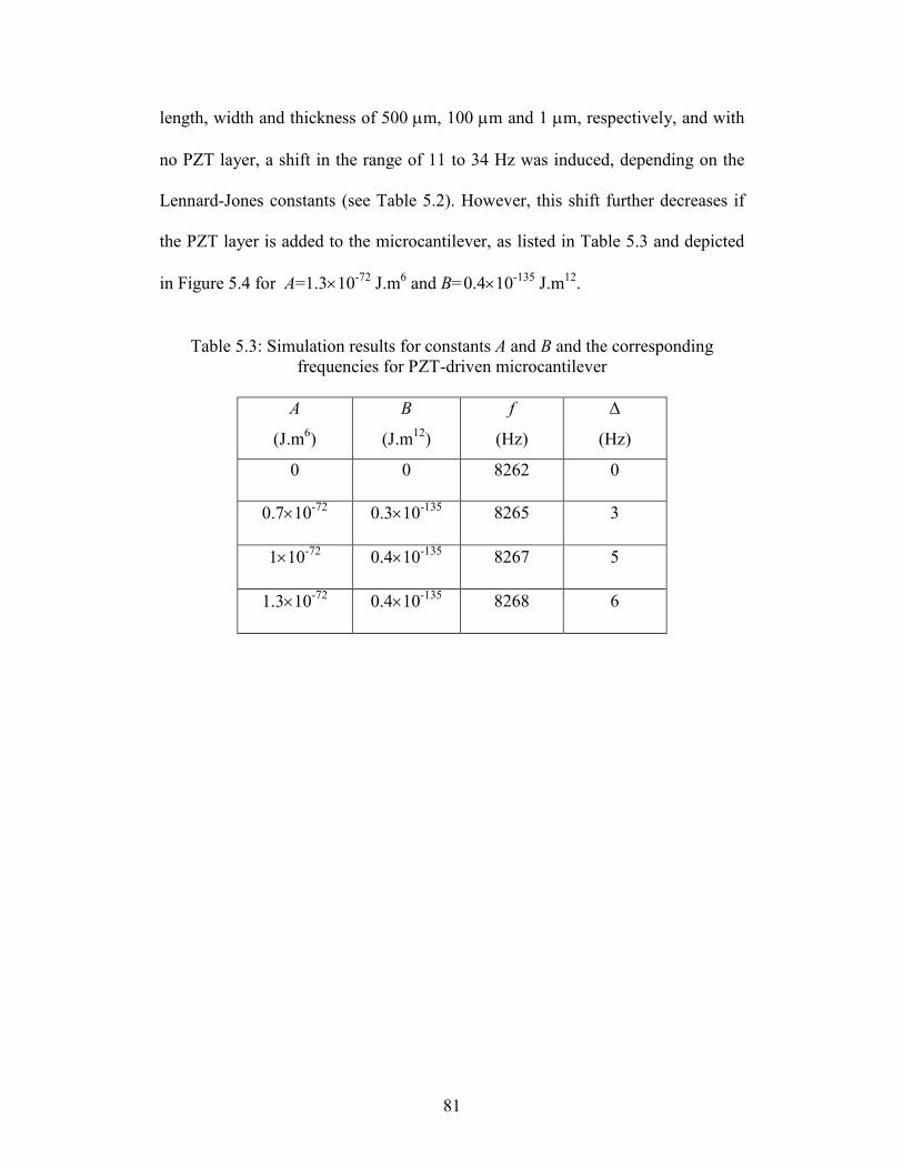
81

length, width and thickness of 500 µm, 100 µm and 1 µm, respectively, and with

no PZT layer, a shift in the range of 11 to 34 Hz was induced, depending on the

Lennard-Jones constants (see Table 5.2). However, this shift further decreases if

the PZT layer is added to the microcantilever, as listed in Table 5.3 and depicted

in Figure 5.4 for A=1.3×10-72 J.m6 and B=0.4×10-135 J.m12

.

Table 5.3: Simulation results for constants A and B and the corresponding

frequencies for PZT-driven microcantilever

A

(J.m6)

B

(J.m12)

f

(Hz)

∆

(Hz)

0 0 8262 0

0.7×10-72 0.3×10-135 8265 3

1×10-72 0.4×10-135 8267 5

1.3×10-72 0.4×10-135 8268 6

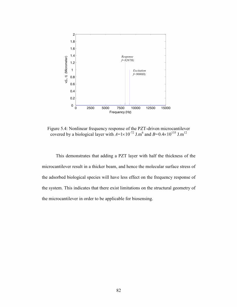
82

0 2500 5000 7500 10000 12500 150000

0.2

0.4

0.6

0.8

1

1.2

1.4

1.6

1.8

2

Frequency (Hz)

v(l

,t)

(Mic

rom

ete

r)

Figure 5.4: Nonlinear frequency response of the PZT-driven microcantilever

covered by a biological layer with A=1×10-72 J.m6 and B=0.4×10135 J.m12

This demonstrates that adding a PZT layer with half the thickness of the

microcantilever result in a thicker beam, and hence the molecular surface stress of

the adsorbed biological species will have less effect on the frequency response of

the system. This indicates that there exist limitations on the structural geometry of

the microcantilever in order to be applicable for biosensing.

Response

f=8267Hz

Excitation

f=9000Hz

v(L, t) (Micrometer)

CHAPTER 6

SENSITIVITY STUDY OF THE STATIC MODE DETECTION

The nonlinear equation of motion of the PZT-driven microcantilever

biosensor of Figure 4.10, Eq. (4.70), was solved in Chapter 5 by first discretizing

the equation of motion and applying the Galerkin method and numerically solving

the derived ordinary differential equations of motion of the microcantilever. In

this Chapter, a new approach is introduced towards the solution of the equation of

motion (4.70). This new approach is utilized in formulating the static deflection of

the microcantilever and as a result, the sensitivity of this formulated static

deflection detection mode is compared to that of the dynamic mode formulated in

Chapter 5.

This method of formulating the static deflection is a powerful method as it

formulates all the intermolecular forces causing the surface stress into the general

equation of motion of the microcantilever. It is easy and straightforward to bring

the forces into the equation of motion of the microcantilever by just knowing its

potential.

84

A New Approach toward Solution of the Nonlinear Equation of Motion of

Eq. (4.70)

The nonlinear vibration of the microcantilever given in Eq. (4.70) can be

considered as the linear vibrations of the microcantilever around its statically

deflected position. In other words, the transversal displacement of the

microcantilever, ( ),v s t , can be written as,

( ) ( )( , ) ,s Linearv s t v s v s t= + (6.1)

where ( )sv s is the static deflection of the beam. The difference between this

method and the method of previous chapter is that the special function φn(s) of the

equation of motion of the vibrating microcantilever is no longer a comparison

function, instead the eigenfunction of the beam satisfying both boundary

conditions and the equation of motion of the linear vibrating beam.

The static deflection of Eq. (6.1) may be easily found by ignoring the

time-varying terms in Eq. (4.70), which results in an equation as follows,

( )( ) ( )( ) ( ) ( ) 3

1 32 4 0s s s s sEI s v v EI s v v A s v A s v′ ′′′ ′ ′′′ ′ ′ ′′ ′ ′ − − + − =

(6.2)

Similar to the assumption made in Chapter 5, it is assumed that

( ) ( ) ( )1 3, andEI s A s A s are constants, hence their derivatives will vanish when

expanding Eq. (6.2).

85

In order to solve Eq. (6.2) and find the static deflection of the

microcantilever beam, Eq. (6.2) needs to be non-dimensionalized first. In this

regard, the new non-dimensional variables x and ˆ ( )sv x are defined as follows,

( ) ( ) 1̂( )s s

sx

L

v s v xL v x⇒ = =

≜ (6.3)

( ) 1̂( )ˆs

v xv x

L≜ (6.4)

Substituting Eqs. (6.3) and (6.4) into Eq. (6.2) and taking the derivatives,

the equation of the static deflection can be rewritten as follows,

( )2 3 2

1 2 3ˆ ˆ ˆ ˆ ˆ ˆ ˆ ˆ ˆ1 4 0s s s s s s s s sB v v v v v v B v B v v ′′′′ ′ ′′ ′′′ ′′ ′ ′′ ′′ ′− + + + + − =

(6.5)

with the boundary conditions of

at x=0 :

ˆ ˆ 0s sv v′= = (6.6)

at x=L:

ˆ ˆ 0s sv v′′ ′′′= = (6.7)

where

86

1 3

EIB

L= (6.8)

12

2AB

L= (6.9)

3

3

12AB

L= (6.10)

Only two of the four boundary conditions listed in Eqs. (6.6) and (6.7) are

available at x=0. Hence, in order to solve Eq. (6.5) the “shooting method” will be

utilized. Using this method, the two unavailable initial conditions at x=0 are

assumed to be known as ( )ˆ 0sv ′′ = α and ( )ˆ 0sv′′′ = β , where α and β are some

constants to be determined. Having all four initial conditions, the static deflection

of the microcantilever may be found numerically based on the following equation,

1

2 1

3 2

4 3

2 33 23 2 3 3 4 3 2

1 1

4 2

2

ˆ

ˆ

ˆ

ˆ

4

ˆ1

s

s

s

s

s

y v

y v y

y v y

y v y

B By y y y y y y

B By v

y

=

′ ′= =

′′ ′= =

′′′ ′= =

− + − − ′ ′′′′= =

+

(6.11)

with the initial conditions as follows,

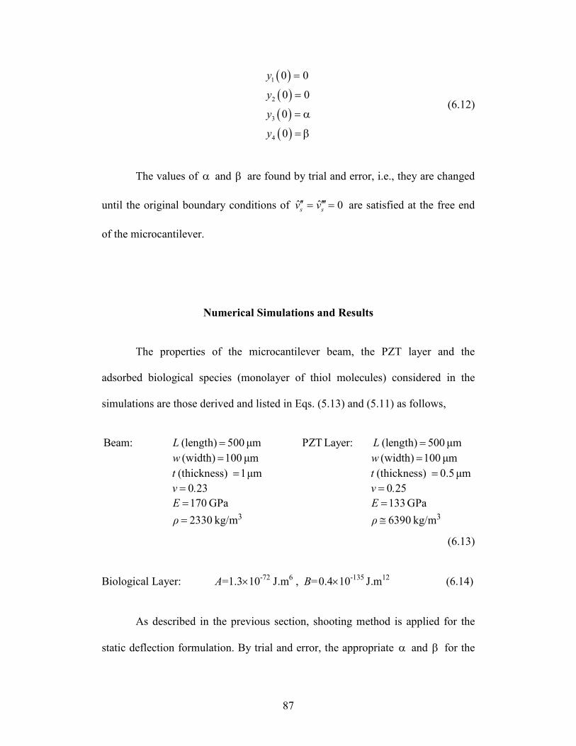
87

( )( )( )( )

1

2

3

4

0 0

0 0

0

0

y

y

y

y

=

=

= α

= β

(6.12)

The values of α and β are found by trial and error, i.e., they are changed

until the original boundary conditions of ˆ ˆ 0s sv v′′ ′′′= = are satisfied at the free end

of the microcantilever.

Numerical Simulations and Results

The properties of the microcantilever beam, the PZT layer and the

adsorbed biological species (monolayer of thiol molecules) considered in the

simulations are those derived and listed in Eqs. (5.13) and (5.11) as follows,

3

Beam: (length) 500 µm

(width) 100 µm

(thickness) 1µm

0 23

170GPa

2330 kg/m

L

w

t

ν .

E

ρ

==

===

=

3

PZTLayer: (length) 500 µm

(width) 100 µm

(thickness) 0.5µm

0 25

133GPa

6390 kg/m

L

w

t

ν .

E

ρ

==

===

≅

(6.13)

Biological Layer: A=1.3×10-72 J.m6 , B=0.4×10-135 J.m12

(6.14)

As described in the previous section, shooting method is applied for the

static deflection formulation. By trial and error, the appropriate α and β for the

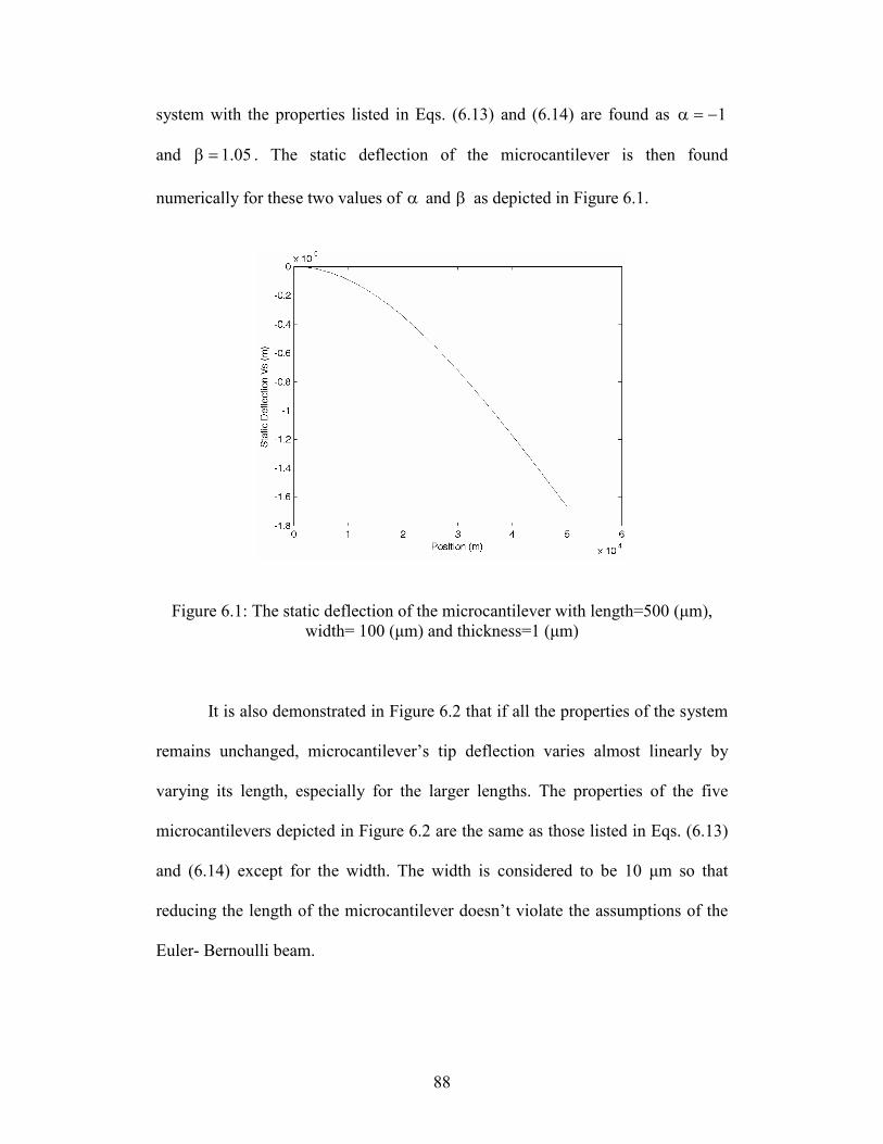
88

system with the properties listed in Eqs. (6.13) and (6.14) are found as 1α = −

and 1.05β = . The static deflection of the microcantilever is then found

numerically for these two values of α and β as depicted in Figure 6.1.

Figure 6.1: The static deflection of the microcantilever with length=500 (µm),

width= 100 (µm) and thickness=1 (µm)

It is also demonstrated in Figure 6.2 that if all the properties of the system

remains unchanged, microcantilever’s tip deflection varies almost linearly by

varying its length, especially for the larger lengths. The properties of the five

microcantilevers depicted in Figure 6.2 are the same as those listed in Eqs. (6.13)

and (6.14) except for the width. The width is considered to be 10 µm so that

reducing the length of the microcantilever doesn’t violate the assumptions of the

Euler- Bernoulli beam.

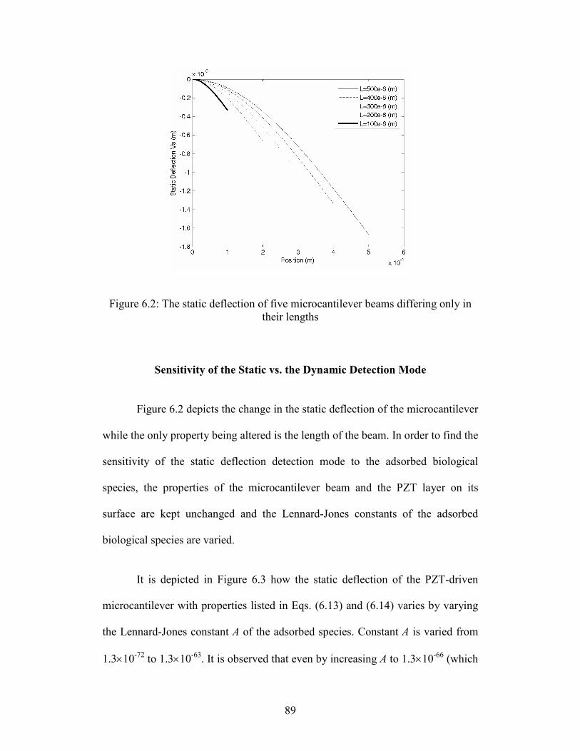
89

Figure 6.2: The static deflection of five microcantilever beams differing only in

their lengths

Sensitivity of the Static vs. the Dynamic Detection Mode

Figure 6.2 depicts the change in the static deflection of the microcantilever

while the only property being altered is the length of the beam. In order to find the

sensitivity of the static deflection detection mode to the adsorbed biological

species, the properties of the microcantilever beam and the PZT layer on its

surface are kept unchanged and the Lennard-Jones constants of the adsorbed

biological species are varied.

It is depicted in Figure 6.3 how the static deflection of the PZT-driven

microcantilever with properties listed in Eqs. (6.13) and (6.14) varies by varying

the Lennard-Jones constant A of the adsorbed species. Constant A is varied from

1.3×10-72 to 1.3×10-63. It is observed that even by increasing A to 1.3×10-66 (which

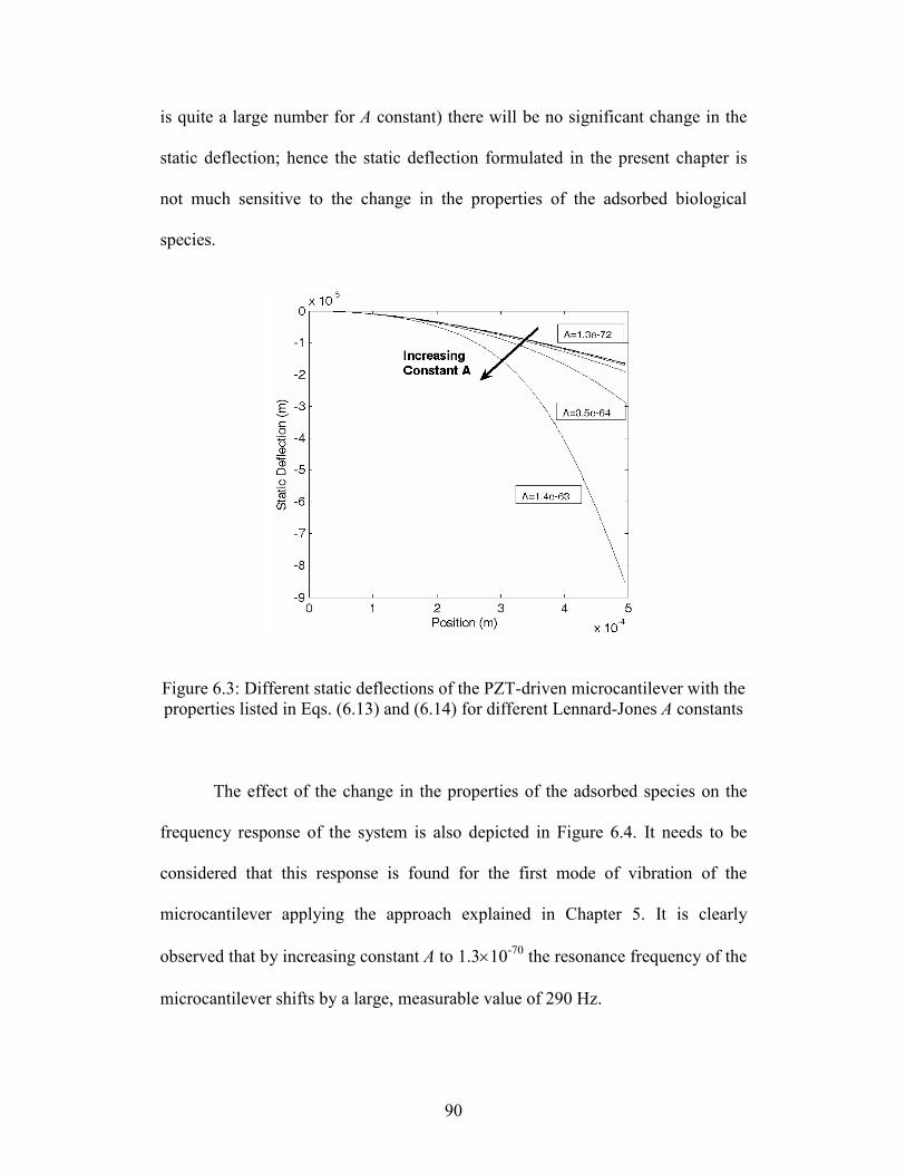
90

is quite a large number for A constant) there will be no significant change in the

static deflection; hence the static deflection formulated in the present chapter is

not much sensitive to the change in the properties of the adsorbed biological

species.

Figure 6.3: Different static deflections of the PZT-driven microcantilever with the

properties listed in Eqs. (6.13) and (6.14) for different Lennard-Jones A constants

The effect of the change in the properties of the adsorbed species on the

frequency response of the system is also depicted in Figure 6.4. It needs to be

considered that this response is found for the first mode of vibration of the

microcantilever applying the approach explained in Chapter 5. It is clearly

observed that by increasing constant A to 1.3×10-70 the resonance frequency of the

microcantilever shifts by a large, measurable value of 290 Hz.

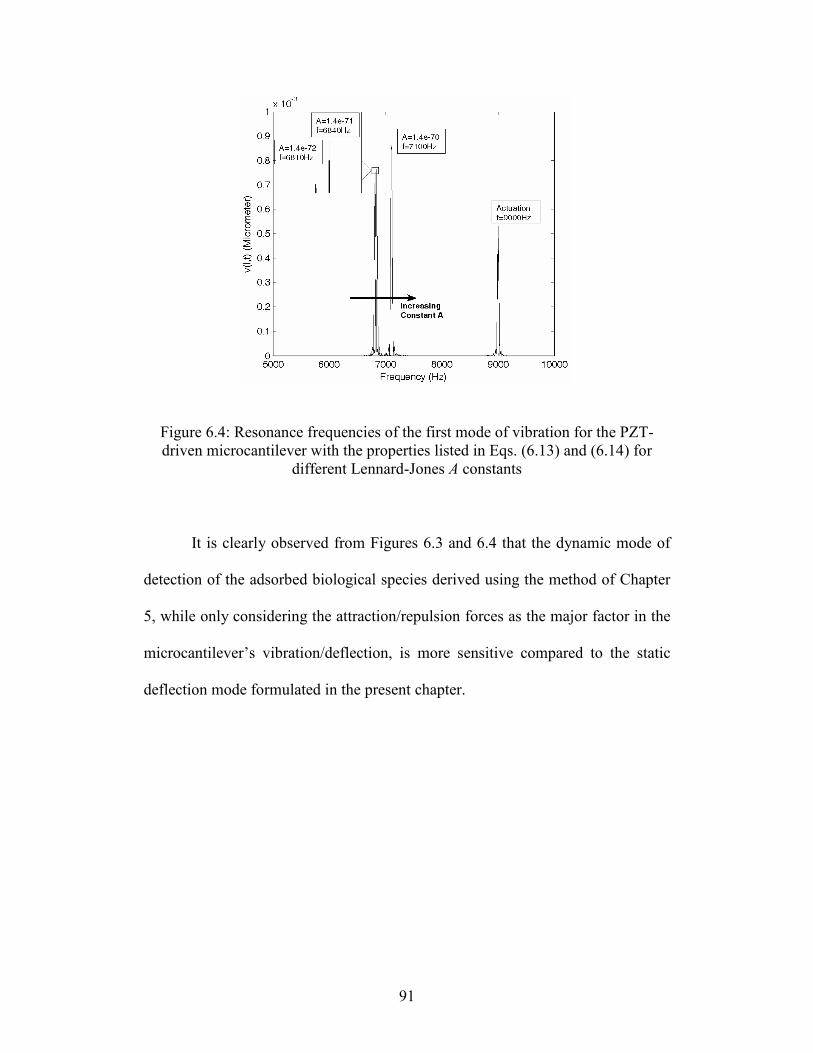
91

Figure 6.4: Resonance frequencies of the first mode of vibration for the PZT-

driven microcantilever with the properties listed in Eqs. (6.13) and (6.14) for

different Lennard-Jones A constants

It is clearly observed from Figures 6.3 and 6.4 that the dynamic mode of

detection of the adsorbed biological species derived using the method of Chapter

5, while only considering the attraction/repulsion forces as the major factor in the

microcantilever’s vibration/deflection, is more sensitive compared to the static

deflection mode formulated in the present chapter.

92

CHAPTER 7

CONCLUSIONS AND FUTURE WORK

Conclusions

Nonlinear vibrations of a piezoelectrically-driven microcantilever beam in

presence of a biological monolayer were investigated and the corresponding

equations of motion were derived and simulated. In formulating the general

equations of motion of the beam, both linear and nonlinear terms due to the

microcantilever’s geometry were present. Moreover, the attached piezoelectric

layer and the adsorbed biological layer produced new nonlinear terms. Two new

nonlinear terms due to presence of these layers were derived and introduced in the

present modeling framework.

It was concluded that the intermolecular forces of attraction/repulsion play

a less dominant role on the adsorption induced surface stress and the resonance

frequency shift. It was then proposed that other effects such as the electrostatic

adhesion forces or the surface charge redistribution of the underlying substrate

may be the contributing factors on the surface stress. It was also observed that

adding the piezoelectric layer causes a great resonance frequency shift from the

initial resonance frequency. Taking the nonlinearities into account causes a small

shift in the resonance frequency of the system. Despite the shift being small

94

compared to the linear shift in resonance frequency, it is in the measurable range

of the microcantilever sensors. Hence, the nonlinear effect of piezoelectric layer

was shown to be important for the resonance response calculations of the system.

In presence of both piezoelectric and biological layers, it was observed that the

addition of piezoelectric layer on the surface of the microcantilever dominates the

effect of intermolecular forces on the resonance frequency shift of the system.

However, piezoelectrically-actuated microcantilever provides the ability of

indirect sensing through this layer, instead of using laser sensor.

In the last phase of the present paper, a new approach was proposed for

equating the static deflection of the microcantilever beam due to the adsorption-

induced surface stress. It was then depicted that the proposed dynamic mode of

detection of the adsorbed biological species derived, while only considering the

attraction/repulsion forces as the major factor in the microcantilever’s

vibration/deflection, is more sensitive compared to the static deflection mode

formulated in the present chapter.

Future Work and Directions

It needs to be noted that the aim of the current study is just to create a new

research pathway for the problem of biologically-induced surface stress sensing

when piezoelectric and geometrical nonlinearities are considered. There is the

need for extensive experiments in order to verify the theoretical and numerical

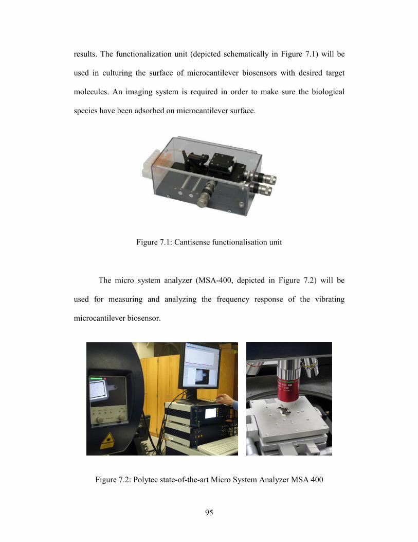
95

results. The functionalization unit (depicted schematically in Figure 7.1) will be

used in culturing the surface of microcantilever biosensors with desired target

molecules. An imaging system is required in order to make sure the biological

species have been adsorbed on microcantilever surface.

Figure 7.1: Cantisense functionalisation unit

The micro system analyzer (MSA-400, depicted in Figure 7.2) will be

used for measuring and analyzing the frequency response of the vibrating

microcantilever biosensor.

Figure 7.2: Polytec state-of-the-art Micro System Analyzer MSA 400

96

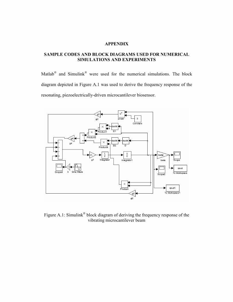
APPENDIX

SAMPLE CODES AND BLOCK DIAGRAMS USED FOR NUMERICAL SIMULATIONS AND EXPERIMENTS

Matlab® and Simulink

® were used for the numerical simulations. The block

diagram depicted in Figure A.1 was used to derive the frequency response of the

resonating, piezoelectrically-driven microcantilever biosensor.

Figure A.1: Simulink® block diagram of deriving the frequency response of the

vibrating microcantilever beam

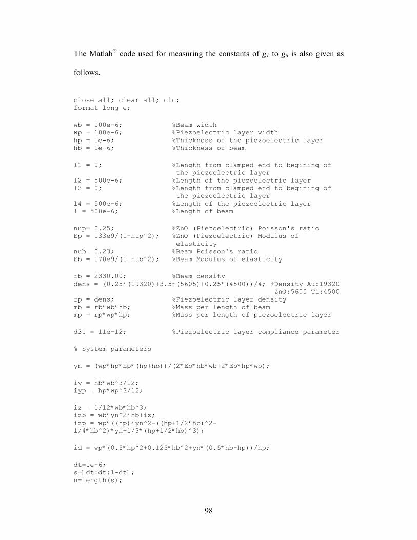
98

The Matlab® code used for measuring the constants of g1 to g6 is also given as

follows.

close all; clear all; clc; format long e;

wb = 100e-6; %Beam width wp = 100e-6; %Piezoelectric layer width hp = 1e-6; %Thickness of the piezoelectric layer hb = 1e-6; %Thickness of beam

l1 = 0; %Length from clamped end to begining of

the piezoelectric layer l2 = 500e-6; %Length of the piezoelectric layer l3 = 0; %Length from clamped end to begining of

the piezoelectric layer l4 = 500e-6; %Length of the piezoelectric layer l = 500e-6; %Length of beam

nup= 0.25; %ZnO (Piezoelectric) Poisson's ratio Ep = 133e9/(1-nup^2); %ZnO (Piezoelectric) Modulus of

elasticity nub= 0.23; %Beam Poisson's ratio Eb = 170e9/(1-nub^2); %Beam Modulus of elasticity

rb = 2330.00; %Beam density dens = (0.25*(19320)+3.5*(5605)+0.25*(4500))/4; %Density Au:19320

ZnO:5605 Ti:4500 rp = dens; %Piezoelectric layer density mb = rb*wb*hb; %Mass per length of beam mp = rp*wp*hp; %Mass per length of piezoelectric layer

d31 = 11e-12; %Piezoelectric layer compliance parameter

% System parameters

yn = (wp*hp*Ep*(hp+hb))/(2*Eb*hb*wb+2*Ep*hp*wp);

iy = hb*wb^3/12; iyp = hp*wp^3/12;

iz = 1/12*wb*hb^3; izb = wb*yn^2*hb+iz; izp = wp*((hp)*yn^2-((hp+1/2*hb)^2-

1/4*hb^2)*yn+1/3*(hp+1/2*hb)^3);

id = wp*(0.5*hp^2+0.125*hb^2+yn*(0.5*hb-hp))/hp;

dt=1e-6; s=[dt:dt:l-dt]; n=length(s);

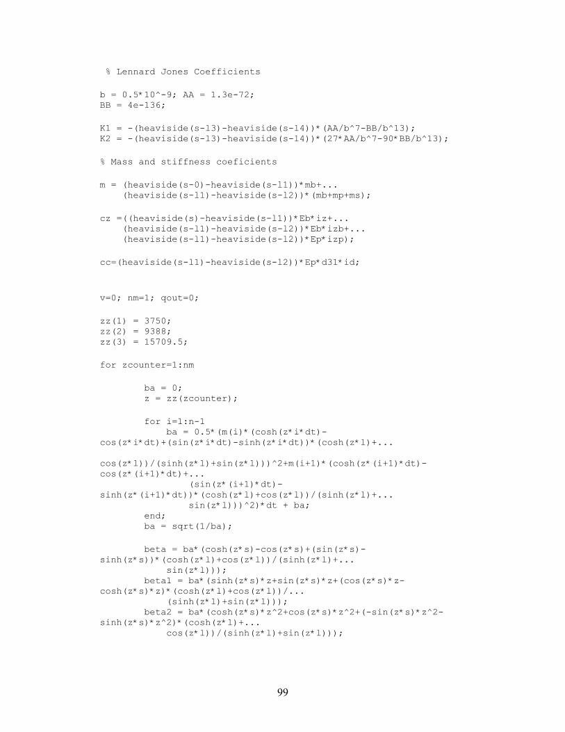
99

% Lennard Jones Coefficients

b = 0.5*10^-9; AA = 1.3e-72; BB = 4e-136;

K1 = -(heaviside(s-l3)-heaviside(s-l4))*(AA/b^7-BB/b^13); K2 = -(heaviside(s-l3)-heaviside(s-l4))*(27*AA/b^7-90*BB/b^13);

% Mass and stiffness coeficients

m = (heaviside(s-0)-heaviside(s-l1))*mb+... (heaviside(s-l1)-heaviside(s-l2))*(mb+mp+ms);

cz =((heaviside(s)-heaviside(s-l1))*Eb*iz+... (heaviside(s-l1)-heaviside(s-l2))*Eb*izb+... (heaviside(s-l1)-heaviside(s-l2))*Ep*izp);

cc=(heaviside(s-l1)-heaviside(s-l2))*Ep*d31*id;

v=0; nm=1; qout=0;

zz(1) = 3750; zz(2) = 9388; zz(3) = 15709.5;

for zcounter=1:nm

ba = 0; z = zz(zcounter);

for i=1:n-1 ba = 0.5*(m(i)*(cosh(z*i*dt)-

cos(z*i*dt)+(sin(z*i*dt)-sinh(z*i*dt))*(cosh(z*l)+...

cos(z*l))/(sinh(z*l)+sin(z*l)))^2+m(i+1)*(cosh(z*(i+1)*dt)-

cos(z*(i+1)*dt)+... (sin(z*(i+1)*dt)-

sinh(z*(i+1)*dt))*(cosh(z*l)+cos(z*l))/(sinh(z*l)+... sin(z*l)))^2)*dt + ba; end; ba = sqrt(1/ba);

beta = ba*(cosh(z*s)-cos(z*s)+(sin(z*s)-

sinh(z*s))*(cosh(z*l)+cos(z*l))/(sinh(z*l)+... sin(z*l))); beta1 = ba*(sinh(z*s)*z+sin(z*s)*z+(cos(z*s)*z-

cosh(z*s)*z)*(cosh(z*l)+cos(z*l))/... (sinh(z*l)+sin(z*l))); beta2 = ba*(cosh(z*s)*z^2+cos(z*s)*z^2+(-sin(z*s)*z^2-

sinh(z*s)*z^2)*(cosh(z*l)+... cos(z*l))/(sinh(z*l)+sin(z*l)));

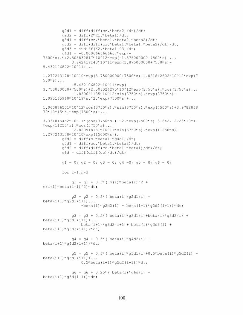
100

g2d1 = diff(diff(cz.*beta2)/dt)/dt; g2d2 = diff(2*K1.*beta1)/dt; g3d1 = diff(cz.*beta1.*beta2.*beta2)/dt; g3d2 = diff(diff(cz.*beta1.*beta1.*beta2)/dt)/dt; g3d3 = 4*diff(K2.*beta1.^3)/dt; g4d1 = -0.0006666666667*exp(-

7500*s).*(2.505832817*10^12*exp(-1.875000000+7500*s)+... 3.842419143*10^11*exp(1.875000000+7500*s)-

5.432106822*10^11+...

1.277243178*10^10*exp(3.750000000+7500*s)+1.081842602*10^12*exp(7

500*s)... +5.432106822*10^11*exp(-

3.750000000+7500*s)+2.506024275*10^12*exp(3750*s).*cos(3750*s)... -1.839661185*10^12*sin(3750*s).*exp(3750*s)-

1.095165960*10^19*s.^2.*exp(7500*s)+...

1.060876501*10^12*cos(3750*s).*sin(3750*s).*exp(7500*s)+3.9782868

79*10^15*s.*exp(7500*s)-...

3.331815452*10^11*(cos(3750*s)).^2.*exp(7500*s)+3.842712723*10^11

*exp(11250*s).*cos(3750*s)... -2.820918181*10^11*sin(3750*s).*exp(11250*s)-

1.277243178*10^10*exp(15000*s)); g4d2 = diff(m.*beta1.*g4d1)/dt; g5d1 = diff(cc.*beta1.*beta2)/dt; g5d2 = diff(diff(cc.*beta1.*beta1)/dt)/dt; g6d = diff(diff(cc)/dt)/dt;

g1 = 0; g2 = 0; g3 = 0; g4 =0; g5 = 0; g6 = 0;

for i=1:n-3

g1 = g1 + 0.5*( m(i)*beta(i)^2 +

m(i+1)*beta(i+1)^2)*dt;

g2 = g2 + 0.5*( beta(i)*g2d1(i) +

beta(i+1)*g2d1(i+1)... -beta(i)*g2d2(i) - beta(i+1)*g2d2(i+1))*dt;

g3 = g3 + 0.5*( beta(i)*g3d1(i)+beta(i)*g3d2(i) +

beta(i+1)*g3d1(i+1)+... beta(i+1)*g3d2(i+1)+ beta(i)*g3d3(i) +

beta(i+1)*g3d3(i+1))*dt;

g4 = g4 + 0.5*( beta(i)*g4d2(i) +

beta(i+1)*g4d2(i+1))*dt;

g5 = g5 + 0.5*( beta(i)*g5d1(i)+0.5*beta(i)*g5d2(i) +

beta(i+1)*g5d1(i+1)+... 0.5*beta(i+1)*g5d2(i+1))*dt;

g6 = g6 + 0.25*( beta(i)*g6d(i) +

beta(i+1)*g6d(i+1))*dt;

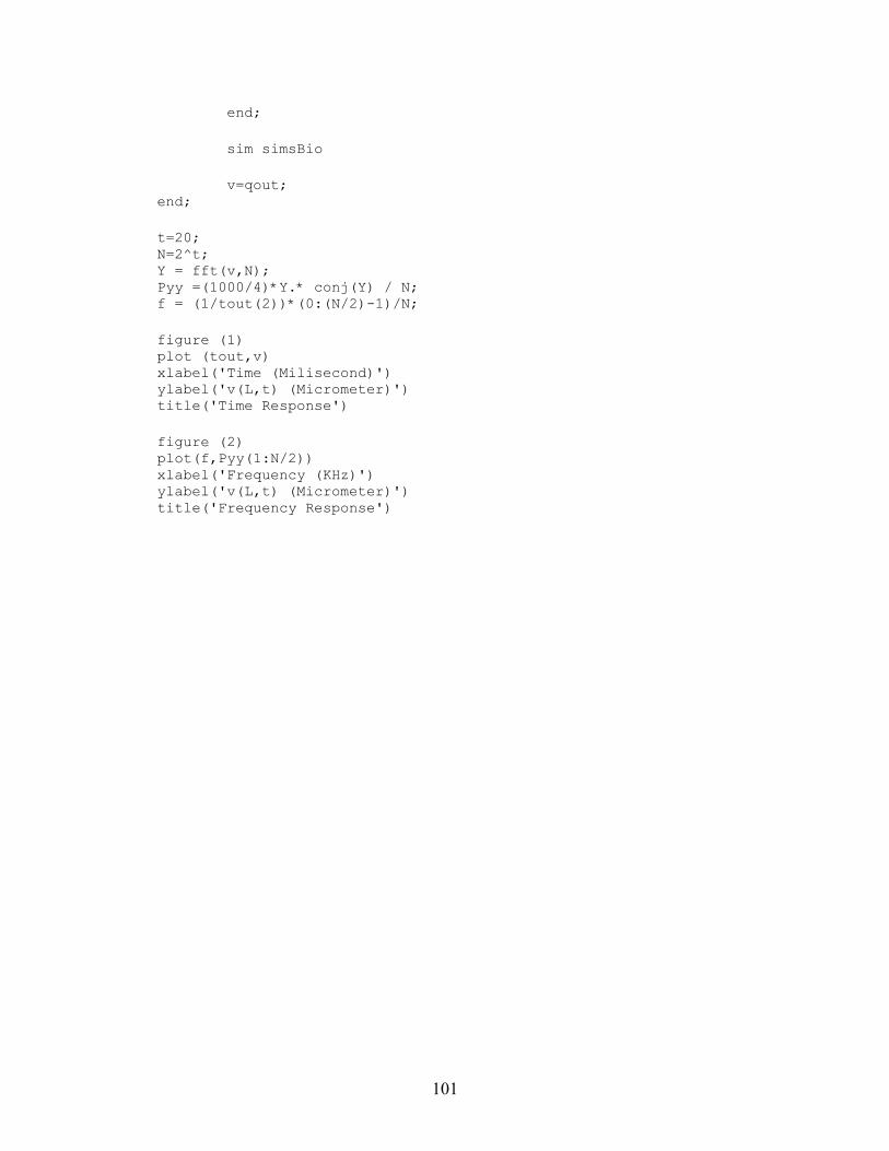
101

end;

sim simsBio

v=qout; end;

t=20; N=2^t; Y = fft(v,N); Pyy =(1000/4)*Y.* conj(Y) / N; f = (1/tout(2))*(0:(N/2)-1)/N;

figure (1) plot (tout,v) xlabel('Time (Milisecond)') ylabel('v(L,t) (Micrometer)') title('Time Response')

figure (2) plot(f,Pyy(1:N/2)) xlabel('Frequency (KHz)') ylabel('v(L,t) (Micrometer)') title('Frequency Response')

102

REFERENCES

[1] Achyuthan K.E., Bergstedt T.S., Chen L., Jones R.M., Kumaraswamy S.,

Kushon S.A., Ley K.D., Lu L., McBranch D., Mukundan H., Rininsland F.,

Shi X., Xia W., and Whitten D.G., “Fluorescence Superquenching of

Conjugated Polyelectrolytes: Applications for Biosensing and Drug

Discovery”, Journal of Materials Chemistry, 15, pp. 2648–2656, 2005.

[2] André P., Vibration Control of Active Structures: An Introduction, Kluwer

Academic Publishers, Netherlands, 1997, Reprinted 1999.

[3] Atkinson, A., “Macro- and Microstress Analysis in Sol-gel Derived

Pb(ZrxTi1-x)O3 Thin Films”, British Ceramic Proceedings, 54, pp. 1-7, 1995.

[4] Barnes J.R., Stephenson R.J., Welland M.E., Gerber Ch., and Gimzewski

J.K., “Photothermal Spectroscopy with Femtojoule Sensitivity Using a

Micromechanical Device”, Nature, 372, pp. 79-81, 1994.

[5] Barnes J.R., Stephenson R.J., Woodburn C.N., O’Shea S.J., Welland M.E.,

Rayment T., Gimzewski J.K., and Gerber Ch., “A Femtojoule Calorimeter

Using Micromechanical Sensors”, Review of Scientific Instruments, 65 (12), pp. 3793-3798, 1994.

[6] Baselt D.R., Lee G.U., and Colton R.J., “Biosensor Based on Force

Microscope Technology”, Journal of Vacuum Science & Technology B, 14 (2), pp. 789-793, 1996.

[7] Baselt D.R., Lee G.U., Hansen K.M., Chrisey L.A., and Colton R.J., “A

High-Sensitivity Micromachined Biosensor”, Proceedings of the IEEE, 85 (4), pp. 672-680, 1997.

[8] Beer F.P., and Johnston E.R, Mechanics of Materials, McGraw-Hill, New

York, 1981.

[9] Berger R., Delamarche E., Lang H.P., Gerber C., Gimzewski J.K., Meyer

E., and Guntherodt H.-J., “Surface Stress in the Self-Assembly of

Alkanethiols on Gold”, Science, 276, pp. 2021–2023, 1997.

104

[10] Berger R., Gerber Ch., and Gimzewski J.K., “Thermal Analysis Using a

Micromechanical Calorimeter”, Applied Physics Letters, 69 (1), pp. 40- 42, 1996.

[11] Britton C.L., Jones R.L., Oden P.I., Hu Z., Warmack R.J., Smith S.F.,

Bryan W.L., and Rochelle J.M., “Multiple-Input Microcantilever Sensors”,

Ultramicroscopy, 82, pp. 17-21, 2000.

[12] Butt H.J., “A Sensitive Method to Measure Changes in the Surface Stress of

Solids”, Journal of Colloid and Interface Science, 180, pp. 251–260, 1996.

[13] Chen G.Y., Thundat T., Wachter E.A., and Warmack R.J., “Adsorption-

Induced Surface Stress and Its Effects on Resonance Frequency of

Microcantilevers”, Journal of Applied Physics, 77 (8), pp. 3618- 3622, 1995.

[14] Cleveland J.P., Manne S., Bocek D., and Hansma P.K., “A Nondestructive

Method for Determining the Spring Constant of Cantilevers for Scanning

Force Microscopy”, Review of Scientific Instruments, 64 (2), pp. 403-405, 1993.

[15] Dadfarnia M., Jalili N., Liu Z., and Dawson D.M., “An Observer-based

Piezoelectric Control of Flexible Cartesian Robot Arms: Theory and

Experiment”, Control Engineering Practice, 12, pp. 1041–1053, 2004.

[16] Dareing D.W., and Thundat T., “Simulation of Adsorption-Induced Stress

of a Microcantilever Sensor”, Journal of Applied Physics, 97, pp. 043526, 2005.

[17] Datskos P.G., Oden P.I., Thundat T., Wachter E.A., Warmack R.J., and

Hunter S.R., “Remote Infrared Radiation Detection Using Piezoresistive

Microcantilevers”, Applied Physics Letters, 69 (20), pp. 2986- 2988, 1996.

[18] Esmailzadeh E., and Jalili N., “Parametric Response of Cantilever

Timoshenko Beams with Tip Mass under Harmonic Support Motion”,

International Journal of Non-Linear Mechanics, 33 (5), pp. 765-781, 1998.

[19] Freund L.B., Floro J.A., and Chason E., “Extensions of the Stoney Formula

for Substrate Curvature to Configurations with Thin Substrates or Large

Deformations”, Applied Physics Letters, 74 (14), pp. 1987-1989, 1999.

105

[20] Fritz J., Baller M.K., Lang H.P., Rothuizen H., Vettiger P., Meyer E.,

Guntherodt H.-J., Gerber Ch., and Gimzewski J.K., “Translating

Biomolecular Recognition into Nanomechanics”, Science, 288, pp. 316- 318, 2000.

[21] Gfeller K.Y., Nugaeva N., and Hegner M., “Rapid Biosensor for Detection

of Antibiotic-Selective Growth of Escherichia coli”, Applied and

Environmental Microbiology, 71 (5), pp. 2626–2631, 2005.

[22] Gimzewski J.K., Gerber Ch., Meyer E., and Schlittler R.R., “Observation of

a Chemical Reaction Using a Micromechanical Sensor”, Chemical Physics

Letters, 217, pp. 589-594, 1994.

[23] Gunter R.L, Zhine R., Delinger W.G., Manygoats K., Kooser A., and Porter

T.L., “Investigation of DNA Sensing Using Piezoresistive Microcantilever

Probes”, IEEE Sensors Journal, 4 (4), pp. 430- 433, 2004.

[24] Gupta A., Akin D., and Bashir R., “Detection of Bacterial Cells and Antibodies using Surface Micromachined Thin Silicon Cantilever

Resonators”, Journal of Vacuum Science & Technology B, 22 (6), pp. 2785-2791, 2004.

[25] Gupta A., Akin D., and Bashir R., “Single Virus Particle Mass Detection

Using Microresonators with Nanoscale Thickness”, Applied Physics Letters,

84 (11), pp. 1976-1978, 2004.

[26] Hansen K.M., Ji H.-F., Wu G., Datar R., Cote R., Majumdar A., and

Thundat T., “Cantilever-Based Optical Deflection Assay for Discrimination

of DNA Single-Nucleotide Mismatches”, Analytical Chemistry, 73 (7), pp. 1567- 1571, 2001.

[27] Ibach H., “The Role of Surface Stress in Reconstruction, Epitaxial Growth and Stabilization of Mesoscopic Structures”, Surface Science Reports, 29, pp. 193-263, 1997.

[28] Ilic B., Craighead H.G., Krylov S., Senaratne W., Ober C., and Neuzil P.

“Attogram Detection Using Nanoelectromechanical Oscillators”, Journal of

Applied Physics, 95 (7), pp. 3694- 3703, 2004.

[29] Ilic B., Yang Y. and Craighead H.G., “Virus detection using

nanoelectromechanical devices”, Applied Physics Letter, 85 (13), pp. 2604- 2606, 2004.

106

[30] Jensenius H., Thaysen J., Rasmussen A.A., Veje L.H., Hansen O., and

Boisen A., “Microcantilever-based Alcohol Vapor Sensor-application and

Response Model”, Applied Physics Letters, 76 (18), pp. 2615-2617 , 2000.

[31] Kirstein K.-U., Li Y., Zimmermann M., Vancura C., Volden T., Song W.H.,

Lichtenberg J., and Hierlemannn A., “Cantilever-based Biosensors in

CMOS Technology”, Proceedings of the Design, Automation and Test in

Europe Conference and Exhibition (DATE’05), pp. 1340-1341, 2005.

[32] Klein, C.A., “How Accurate Are Stoney’s Equation and Recent

Modifications”, Journal of Applied Physics, 88 (9), pp. 5487- 5489, 2000.

[33] Klein C.A., and Miller R., “Strains and Stresses in Multilayered Elastic

Structures: The Case of Chemically Vapor-Deposited ZnS/ZnSe

Laminates”, Journal of Applied Physics, 87, pp. 2265-2272, 2000.

[34] Koch R., and Abermann R., “On the Influence of Thermal Effects on

Internal Stress Measurements during and After Deposition of Silver, Gold

and Copper Films”, Thin Solid Films, 129, PP. 63-70, 1985.

[35] Lai L., Perazzo T., Shi Z., and Majumdar A., “Optimization and

Performance of High-resolution Micro-optomechanical Thermal Sensor”,

Sensors and Actuators A, 58, pp. 113-119, 1997.

[36] Lang H.P., Berger R., Battiston F., Ramseyer J.-P., Meyer E., Andreoli C.,

Brugger J., Vettiger P., Despont M., Mezzacasa T., Scandella L.,

Güntherodt H.-J., Gerber Ch., and Gimzewski J.K., “A Chemical Sensor

Based on a Micromechanical Cantilever Array for the Identification of

Gases and Vapors”, Applied Physics A, 66 (7), pp. S61-S64, 1998.

[37] Lavrik N.V., Sepaniak M.J., and Datskos P.G., “Cantilever Transducers as a

Platform for Chemical and Biological Sensors”, Review of Scientific

Instruments, 75 (7), pp. 2229- 2253, 2004.

[38] Lee J.H., Kim T.S., and Yoon K.H., “Effect of mass and stress on resonant

frequency shift of functionalized Pb(Zr0.52Ti0.48)O3 thin film microcantilever

for the detection of C-reactive protein”, Applied Physics Letter, 84 (16), pp. 3187-3189, 2004.

[39] Lu P., Shen F., O’Shea S.J., Lee K.H., and Ng T.Y., “Analysis of Surface Effects on Mechanical Properties of Microcantilevers”, Materials Physics

and Mechanics, 4, pp. 51–55, 2001.

107

[40] Mahmoodi S.N., Khadem S.E., and Jalili N., “Theoretical Development and

Closed-form Solution of Nonlinear Vibrations of a Directly Excited

Nanotube-reinforced Composite Cantilevered Beam”, Archive of Applied

Mechanics, 75, pp. 153–163, 2006.

[41] Martinez R.E., Augustyniak W.M., and Golovchenko J.A., “Direct

Measurement of Crystal Surface Stress”, Physical Review Letters, 64 (9), pp. 1035-1038, 1990.

[42] McFarland A., Poggi M., Doyle M., Bottomley L., and Colton J., “Influence

of Surface Stress on the Resonance Behavior of Microcantilevers”, Applied

Physics Letters, 87, pp. 053505, 2005.

[43] Miyatani T., and Fujihira M., “Calibration of Surface Stress Measurements

with Atomic Force Microscopy”, Journal of Applied Physics, 81 (11), pp. 7099-7115, 1997.

[44] Oden P.I., “Gravimetric Sensing of Metallic Deposits Using an End-loaded

Microfabricated Beam Structure”, Sensors and Actuators B, 53, pp. 191–196, 1998.

[45] Oden P.I., Chen G.Y. , Steele R.A., Warmack R.J., and Thundat T.,

“Viscous Drag Measurements Utilizing Microfabricated Cantilevers”,

Applied Physics Letters, 68 (26), pp. 3814- 3816, 1999.

[46] Oden P.I., Datskos P.G., Thundat T., and Warmack R.J., “Uncooled

Thermal Imaging Using a Piezoresistive Microcantilever”, Applied Physics

Letters, 69 (21), pp. 3277-3279, 1996.

[47] Patel S.S., and Tirrel M., “Measurement of Forces between Surfaces in

Polymer Fluids”, Annual Review of Physical Chemistry, 40, pp. 597–635, 1989.

[48] Perazzo T., Mao M., Kwon O., Majumdar A., Varesi J.B, and Norton P.,

“Infrared Vision Using Uncooled Micro-optomechanical Camera”, Applied

Physics Letters, 74 (23), pp. 3567- 3569, 1999.

[49] Raiteri R., and Butt H.-J., “Measuring Electrochemically Induced Surface

Stress with an Atomic Force Microscope”, Journal of Physical Chemistry,

99, pp. 15728-15732, 1995.

108

[50] Ren Q., and Zhao Y.-P., “Influence of Surface Stress on Frequency of Microcantilever-based Biosensors”, Microsystem Technologies, 10, pp. 307-314, 2004.

[51] Sader J.E., “Surface Stress Induced Deflections of Cantilever Plates with Applications to the Atomic Force Microscope: Rectangular Plates”, Journal

of Applied Physics, 89 (5), pp. 2911-2921, 2001.

[52] Sader J.E., Larson I., Mulvaney P., and White L.R., “Method for the

Calibration of Atomic Force Microscope Cantilevers”, Review of Scientific

Instruments, 66 (7), pp. 3789-3798, 1995.

[53] Savran C.A., Knudsen S.M., Ellington A.D., and Manalis S.R.,

“Micromechanical Detection of Proteins Using Aptamer-Based Receptor

Molecules”, Analytical Chemistry, 76, pp. 3194-3198, 2004.

[54] Schell-Sorokin A.J., and Tromp, R.M., “Mechanical Stress in (Sub)-

monolayer Epitaxial Films”, Physical Review Letters, 64 (9), pp. 1039, 1990.

[55] Sepaniak M., Datskos P., Lavrik N., and Tipple C., “Microcantilever

Transducers: A New Approach in Sensor Technology”, Analytical

Chemistry, 74 (21), pp. 568 A-575 A, 2002.

[56] Shuttleworth R., “The Surface Tension of Solids”, Proceedings of the Physical Society, 63 (5), pp. 444-457, 1950.

[57] Sitti M., and Hashimoto H., “Controlled Pushing of Nanoparticles:

Modeling and Experiments”, IEEE/ASME Transactions on Mechatronics, 5 (2), pp. 199-211, 2000.

[58] Stokes R.J., and Evans D.F., Fundamentals of Interfacial Engineering, Wiley–VCH, New York, 1997.

[59] Stoney G.G., “The tension of Metallic Films Deposited by Electrolysis”,

Proceedings of the Royal Society of London A, 82, pp. 172-175, 1909.

[60] Su M., Li S., and Dravid V.P., “Microcantilever Resonance-based DNA

Detection with Nanoparticle Probes”, Applied Physics Letter, 82 (20), pp. 3562- 3564, 2003.

109

[61] Subramanian A., Oden P.I., Kennel S.J., Jacobson K.B., Warmack R.J.,

Thundat T., and Doktycz M.J., “Glucose Biosensing using an Enzyme-

coated Microcantilever”, Applied Physics Letter, 81 (2), pp. 385- 387, 2002.

[62] Taylor E.H., and Waggener W.C., “Measurement of Adsorptive Forces”,

Journal of Physical Chemistry, 83 (10), pp. 1361-1362, 1979.

[63] Thundat T., Chen G.Y., Warmack R.J., Allison D.P., and Wachter E.A.

“Vapor Detection Using Resonating Microcantilevers”, Analytical

Chemistry, 67, pp. 519-521, 1995.

[64] Thundat T., Oden P.I., and Warmack R.J., “Microcantilever Sensors”,

Microscale Thermophysical Engineering, 1, pp. 185-199, 1997.

[65] Thundat T., Wachter E.A., Sharp S.L., and Warmack R.J., “Detection of

Mercury Vapor Using Resonating Microcantilevers”, Applied Physics

Letters, 66 (13), pp. 1695- 1697, 1995.

[66] Thundat T., Warmack R.J., Chen G.Y., and Allison D.P., “Thermal and

Ambient-induced Deflections of Scanning Force Microscope Cantilevers”,

Applied Physics Letters, 64 (21), pp. 2894- 2898, 1994.

[67] Townsend P.H., Barnett D.M., and Brunner T.A., “Elastic Relationship in

Layered Composite Media with Approximation for the Case of Thin Films

on a Thick Substrate”, Journal of Applied Physics, 62 (11), pp. 4438-4444, 1987.

[68] Wachter E.A., and Thundat T., “Micromechanical Sensors for Chemical

and Physical Measurements”, Review of Scientific Instruments, 66 (6), pp. 3662- 3667, 1995.

[69] Wachter E.A., Thundat T., Oden P.I., Warmack R.J., Datskos P.G., and

Sharp S.L., “Remote Optical Detection Using Microcantilevers”, Review of

Scientific Instruments., 67 (10), pp. 3434- 3439, 1996.

[70] Weigert S., Dreier M., and Hegner M., “Frequency Shifts of Cantilevers

Vibrating in Various Media”, Applied Physics Letters, 69 (19), pp. 2834- 2836, 1996.

[71] Wu G., Ji H., Hansen K., Thundat T., Datar R., Cote R., Hagan M.F.,

Chakraborty A.K., and Majumdar A., “Origin of Nanomechanical

Cantilever Motion Generated from Biomolecular Interactions”, Proceedings

of the National Academy of Sciences, 98 (4), pp. 1560–1564, 2001.

110

[72] Yu N., and Polycarpou A.A., “Adhesive Contact Based on the Lennard–Jones Potential: A Correction to the Value of the Equilibrium Distance as

Used in the Potential”, Journal of Colloid and Interface Science, 278, pp. 428–435, 2004.

[73] Zhang W., and Turner K., “Frequency-Tuning for Control of Parametrically

Resonant Mass Sensors”, Journal of Vacuum Science and Technology A, 23 (4), pp. 841-845, 2005.

[74] Zhang Y., Ren Q., and Zhao Y., “Modeling Analysis of Surface Stress on a

Rectangular Cantilever Beam”, Journal of Physics D: Applied Physics, 37, pp. 2140–2145, 2004.

[75] Zhou X.C., O’Shea S.J., and Sam Fong Yau Li, “Amplified

Microgravimetric Gene Sensor using Au Nanoparticle Modified

Oligonucleotides”, Chemical Communications, pp. 953–954, 2000.

[76] http://www.pharmaceutical-int.com/categories/qcm-technology/quartz-

crystal-microbalance-qcm.asp

[77] http://www.q-sense.com

[78] http://www.masscal.com/instrument.html