NONLINEAR MODELING OF INERTIAL ERRORS BY FAST ORTHOGONAL

NONLINEAR MODELING OF INERTIAL ERRORS BY FAST

ORTHOGONAL SEARCH ALGORITHM FOR LOW COST

VEHICULAR NAVIGATION

by

Zhi Shen

A thesis submitted to the Department of Electrical and Computer Engineering

In conformity with the requirements for

the degree of Doctor of Philosophy

Queen’s University

Kingston, Ontario, Canada

January, 2012

Copyright © Zhi Shen, 2012

ii

Abstract

Due to their complementary characteristics, Global Positioning System (GPS) is usually

integrated with standalone navigation devices like odometers and inertial measurement units

(IMU). Recently, intensive research has focused on utilizing Micro-Electro-Mechanical-System

(MEMS) grade inertial sensors in the integration because of their low cost. In this study, a

reduced inertial sensor system (RISS) is considered. It comprises a MEMS grade single axis

gyroscope, the vehicle built-in odometer, and two optional MEMS grade accelerometers.

Estimation technique is needed to allow the data fusion of RISS and GPS. With adequate

accuracy, Kalman filter (KF) fulfills this requirement if high-end inertial sensors are used.

However, due to the inherent error characteristics of MEMS devices, MEMS-based RISS suffers

from the non-stationary stochastic sensor errors and nonlinear inertial errors, which cannot be

suppressed by KF alone. To solve the problem, Fast Orthogonal Search (FOS), a nonlinear

system identification algorithm, is suggested in this research for modeling higher order RISS

errors. FOS algorithm has the ability to figure out the system nonlinearity with a tolerance of

arbitrary stochastic system noise. Its modeling results can then be used to predict the system

dynamics. Motivated by the above merits, a KF/FOS module is proposed. By handling both linear

and nonlinear RISS errors, this module targets substantial enhancement of positioning accuracy.

To examine the effectiveness of the proposed technique, KF/FOS module is applied on RISS with

GPS in a land vehicle for several road test trajectories. Its performance is compared to KF-only

method, both assessed with respect to a high-end reference. To evaluate navigation algorithm in

real-time vehicle application, a multi-sensor data logger is designed in this research to collect

online RISS/GPS data. KF/FOS module is transplanted on an embedded digital signal processor

as well. Both the off-line and online results confirm that KF/FOS module outperforms KF-only

approach in positioning accuracy. They also demonstrate reliable real-time performance.

iii

Acknowledgements

I would like to express my sincere gratitude to my supervisors: Dr. Noureldin and Dr. Korenberg.

I am grateful to Dr. Noureldin for his guidance, patience, encouragement, and strong support

during my PhD program. Dr. Noureldin directs me to enter the realm of multi-sensor integration

and inertial navigation. Over four years, I have benefited and learnt a lot from his creative ideas,

insightful advices, and exceptional foresight. This thesis shall never be accomplished without his

invaluable helps. I am also indebted to my co-supervisor, Dr. Korenberg, for his significant

support and encouragement. Dr. Korenberg introduced me to the topic of fast orthogonal search

and offered important guideline throughout my study. I am very proud and pleased to have my

research work supervised by Dr. Noureldin and Dr. Korenberg.

I also highly appreciate all my colleagues at Navigation and Instrumentation (NavINST) research

group led by Dr. Noureldin. Their sincere suggestions, professional spirit, and outstanding team

work let me enjoy working in the NavINST family. Special thanks are due to my colleagues and

friends: Dr. Jacques Georgy, Mr. Umar Iqbal, and Mr. Tashfeen Karamat. Jacques provided the

initial KF-based 3D RISS/GPS solution. His profound insight and knowledge offered great helps

in my PhD research and thesis writing. We also cooperated in collecting data of most road test

trajectories presented in this paper. Umar provided the original KF-based 2D RISS/GPS solution.

He also clarified a lot of RISS details to me. Tashfeen's expertise on Kalman filter is always so

helpful to refer. We also cooperated in several road test experiments. I would like to thank Mr.

Ali Massoud, Mr. Scott Dybwad, and Mr. Walid Farid Abd El Fatah as well. Ali and Scott

provided important suggestions on applying fast orthogonal search algorithm into specific fields.

Walid assisted me on developing the hardware and firmware of the multi-sensor data logger. I

also appreciate Capt. Julie Perreault, Capt. Eric North, and LCdr. Lepinsy Chanthalansy for their

collaboration in collecting data of several road test trajectories.

iv

This research was supported in part by Mobile Multi-Sensor System research group in the

department of Geomatics Engineering at University of Calgary (led by Dr. Naser El-Sheimy) and

Trusted Positioning Inc. (led by Dr. Chris Goodall). They provided hardware resource including

ultra-low-cost MEMS grade inertial sensors and printed circuit board fabrication. Without their

helps, it is impossible to prototype the multi-sensor data logger. I also appreciate them for sharing

the dataset they collected in downtown Calgary. Moreover, I would like to thank department of

Electrical and Computer engineering at Queen's University and Royal Military College for their

sustained support throughout my PhD program.

My parents' love supported me in my entire life including this thesis work. Their encouragement

inspired me to overcome every difficulty in my study. No words can describe how grateful I am

to my mother and father.

v

Table of Contents

Abstract ............................................................................................................................................ ii

Acknowledgements ......................................................................................................................... iii

Table of Contents ............................................................................................................................. v

List of Figures ............................................................................................................................... viii

List of Tables ................................................................................................................................. xii

Glossary ........................................................................................................................................ xiii

Chapter 1 Introduction .................................................................................................................... 1

1.1 Overview ................................................................................................................................ 1

1.2 Problem Statement ................................................................................................................. 2

1.3 Research Motivation and Objectives ..................................................................................... 3

1.4 Research Contribution ........................................................................................................... 5

1.5 Dissertation Outline ............................................................................................................... 7

Chapter 2 Overview of Navigation Systems ................................................................................. 10

2.1 Categories of Navigation Approaches ................................................................................. 10

2.1.1 Dead Reckoning Systems ............................................................................................. 10

2.1.2 Reference-based Absolute Solutions ............................................................................ 12

2.2 Inertial Navigation System .................................................................................................. 15

2.2.1 Principle of Inertial Navigation ..................................................................................... 15

2.2.2 Introduction of Reference Frames ................................................................................. 17

2.2.3 Overview of INS errors ................................................................................................. 19

2.3 GNSS Solution ..................................................................................................................... 20

2.3.1 Overview of Existing GNSS ......................................................................................... 20

2.3.2 Positioning Mechanism of GPS .................................................................................... 21

2.3.3 GPS Signal Characteristics ........................................................................................... 23

2.4 INS/GPS Integration ............................................................................................................ 25

2.4.1 Benefits of INS/GPS Integration ................................................................................... 25

2.4.2 Types of INS/GPS Integration ...................................................................................... 27

2.4.3 Methodologies of INS/GPS Data Fusion ...................................................................... 29

Chapter 3 Analysis of Inertial Navigation System Errors ............................................................. 31

3.1 Three Dimensional INS ....................................................................................................... 31

3.1.1 Structure of 3D INS ...................................................................................................... 31

vi

3.1.2 Equations of 3D INS Mechanization ............................................................................ 33

3.1.3 Dynamic Error Model of 3D INS ................................................................................. 35

3.1.4 Nonlinearity of INS Errors ............................................................................................ 43

3.2 Reduced Inertial Sensor System .......................................................................................... 45

3.2.1 Two Dimensional Reduced Inertial Sensor System ...................................................... 45

3.2.2 Three Dimensional Reduced Inertial Sensor System .................................................... 47

3.2.3 Error Modeling of Reduced Inertial Sensor System ..................................................... 51

3.3 Kalman Filter Based INS/GPS Integration .......................................................................... 54

3.3.1 Kalman Filter and INS/GPS Data Fusion ..................................................................... 54

3.3.2 Limitation of KF-based INS/GPS Integration............................................................... 60

3.3.3 Current State of the Art Methods .................................................................................. 61

Chapter 4 Fast Orthogonal Search Algorithm ............................................................................... 65

4.1 Review of Fast Orthogonal Search (FOS) ........................................................................... 65

4.2 Polynomial Representation of Nonlinear System ................................................................ 66

4.3 Implicit Gram-Schmidt Orthogonal Search of Candidates .................................................. 67

4.4 Merits of FOS Algorithm ..................................................................................................... 71

Chapter 5 Cascade of Kalman Filter and Fast Orthogonal Search for MEMS – Based INS/GPS

Integration ...................................................................................................................................... 73

5.1 Augmented KF/FOS Module ............................................................................................... 73

5.1.1 Modeling Stage ............................................................................................................. 73

5.1.2 Prediction Stage ............................................................................................................ 75

5.2 Two Dimensional Vehicular Navigation using KF/FOS Module ........................................ 76

5.2.1 Experimental Setup of 2D RISS ................................................................................... 76

5.2.2 The First Trajectory ...................................................................................................... 82

5.2.3 The Second Trajectory .................................................................................................. 93

5.2.4 The Third Trajectory ................................................................................................... 100

5.3 Three Dimensional Vehicular Navigation using KF/FOS Module .................................... 103

5.3.1 Experimental Setup of 3D RISS ................................................................................. 103

5.3.2 The Fourth Trajectory ................................................................................................. 106

5.3.3 The Fifth Trajectory .................................................................................................... 113

Chapter 6 Front-End Multi-Sensor Data Logger ......................................................................... 118

6.1 Hardware Description ........................................................................................................ 119

6.1.1 Ublox GPS Receiver Chipset ...................................................................................... 120

vii

6.1.2 MEMS Grade IMU from Analog Devices .................................................................. 121

6.1.3 External Interfaces for OBD-II and Hosts .................................................................. 123

6.1.4 CPU and SD Card Storage .......................................................................................... 124

6.2 Firmware / Software Design .............................................................................................. 126

6.2.1 Multi-Task Scheduling and Synchronization .............................................................. 126

6.2.2 Protocol Design of the Unified Uploading Packet ...................................................... 131

6.2.3 Host Software .............................................................................................................. 133

6.3 Experiment Results ............................................................................................................ 135

Chapter 7 Real-time Design of FOS-based Modeling of Nonlinear Inertial Errors.................... 141

7.1 Objective ............................................................................................................................ 141

7.2 DSP-based Hardware Implementation of KF/FOS Module............................................... 143

7.2.1 Platform Selection ....................................................................................................... 143

7.2.2 System Architecture .................................................................................................... 152

7.2.3 Experimental Setup ..................................................................................................... 154

7.3 Road Test Results and Discussion ..................................................................................... 156

Chapter 8 Conclusions and Future Work ..................................................................................... 161

8.1 Conclusions ........................................................................................................................ 161

8.2 Recommendations of Future Work .................................................................................... 164

References .................................................................................................................................... 167

Appendix I – Structure of Data Logger’s GPS / Sensor Data Packets ......................................... 173

Appendix II – Publication List ..................................................................................................... 175

viii

List of Figures

Fig. 2-1: Capacitance sensing structure (comb fingers) of InvenSense gyro IDG – 300 [16] ....... 17

Fig. 2-2: Structure of body level frame .......................................................................................... 18

Fig. 2-3: Structure of local level frame .......................................................................................... 19

Fig. 2-4: Location of GPS receiver using trilateration principle .................................................... 22

Fig. 2-5: Multipath effects of GPS signals ..................................................................................... 24

Fig. 2-6: Structure of loosely coupled INS/GPS integration ......................................................... 27

Fig. 2-7: Structure of tightly coupled INS/GPS integration ........................................................... 27

Fig. 3-1: Setup of gyroscopes and accelerometers of a full IMU in a body level frame ............... 31

Fig. 3-2: Concept and procedure of 3D INS mechanization .......................................................... 32

Fig. 3-3: Bias offset and bias drift of an inertial sensor ................................................................. 38

Fig. 3-4: Autocorrelation sequence of the first order Gauss Markov model.................................. 40

Fig. 3-5: Autocorrelation sequence of KVH E-Core2000 fiber optic gyroscope measurements

using 3-hour static data .................................................................................................................. 41

Fig. 3-6: Block diagram of the first order GM model shaping filter .............................................. 41

Fig. 3-7: Autocorrelation sequence of a first order Gauss Markov process in case of different

correlation parameters .............................................................................................................. 42

Fig. 3-8: Setup of the gyroscope and odometer of a 2D RISS in a body level frame .................... 46

Fig. 3-9: Block diagram of 2D RISS mechanization ..................................................................... 46

Fig. 3-10: Setup of the gyroscope, odometer, and accelerometers of 3D RISS ............................. 48

Fig. 3-11: Gravity effects on the forward direction caused by the pitch angle .............................. 49

Fig. 3-12: Normal part of vehicle acceleration and gravity effects on the transversal direction

caused by the roll angle.................................................................................................................. 49

Fig. 3-13: Block diagram of 3D RISS mechanization ................................................................... 51

Fig. 3-14: Block diagram of KF-based INS/GPS integration ........................................................ 55

Fig. 3-15: Two major stages in KF: prediction and update ........................................................... 58

Fig. 3-16: Recursive scheme of Kalman filtering .......................................................................... 59

Fig. 3-17: P-δP structure of Neural Network based INS/GPS integration .................................... 63

Fig. 4-1: Block diagram of Fast Orthogonal Search algorithm ...................................................... 70

Fig. 5-1: Modeling stage of KF/FOS module during GPS availability .......................................... 74

Fig. 5-2: Prediction stage of KF/FOS module during GPS outages .............................................. 75

Fig. 5-3: Crossbow IMU300CC-100 [77] ...................................................................................... 77

ix

Fig. 5-4: CarChip® driving and engine performance monitor from Davis Instruments [76] ........ 77

Fig. 5-5: Honeywell HG1700 tactical grade 6DOF IMU [78] ....................................................... 79

Fig. 5-6: NovAtel’s ProPak-G2 plus GNSS receiver [78] ............................................................. 79

Fig. 5-7: Block diagram of the experimental platform for 2D vehicle navigation tests ................ 80

Fig. 5-8: Installation of the equipment inside the van for 2D road tests ........................................ 81

Fig. 5-9: Road test trajectory between Kingston and Napanee. Circles indicate the location of

GPS outages. .................................................................................................................................. 83

Fig. 5-10: (A) Maximum position error and (B) RMS position error during 60-second GPS

outages in the first trajectory .......................................................................................................... 85

Fig. 5-11: Maximum azimuth errors during 60-second GPS outages of the first trajectory .......... 86



Fig. 5-13: Positioning results during GPS outage #4 of the first trajectory ................................... 89

Fig. 5-14: The vehicle’s speed and azimuth during GPS outage #4 of the first trajectory ............ 90

Fig. 5-15: Positioning results in GPS outage #6 of the first trajectory .......................................... 91


Fig. 5-17: Positioning results during GPS outage #8 of the first trajectory ................................... 93


Fig. 5-19: Road test trajectory in the suburbs of Kingston, Ontario. Circles indicate the locations

of GPS outages. .............................................................................................................................. 94


outages in the second trajectory ..................................................................................................... 95

Fig. 5-21: Positioning results during GPS outage #3 of the second trajectory .............................. 96

Fig. 5-22: The vehicle’s speed and azimuth during GPS outage #3 of the second trajectory ........ 97

Fig. 5-23: Positioning error of KF-only and KF/FOS vs. Time in GPS outage #3 ........................ 97

Fig. 5-24: Positioning results during GPS outage #4 of the second trajectory .............................. 99

Fig. 5-25: The vehicle’s speed and azimuth during GPS outage #4 of the second trajectory ...... 100

Fig. 5-26: Road test trajectory in downtown Kingston. Circles indicate the locations of GPS

outages. ........................................................................................................................................ 101


outages in the third trajectory ...................................................................................................... 103

Fig. 5-28: Installation of the equipment inside the van for 3D road tests .................................... 105

x

Fig. 5-29: Road test trajectory in downtown Toronto. Circles indicate the locations of GPS

outages. ........................................................................................................................................ 107


outages in the fourth trajectory .................................................................................................... 109

Fig. 5-31: Positioning results during GPS outage #1 of the fourth trajectory .............................. 110

Fig. 5-32: The vehicle’s speed and azimuth during GPS outage #1 of the fourth trajectory ....... 110

Fig. 5-33: The vehicle’s pitch and roll during GPS outage #1 of the fourth trajectory ............... 111

Fig. 5-34: Time stamp of KF/FOS and KF-only when their position errors exceed 5 meters in

GPS outages of trajectory #4 ....................................................................................................... 112

Fig. 5-35: Road test trajectory from Kingston to Jones Falls, Ontario, Canada. Circles indicate the

locations of GPS outages. ............................................................................................................ 114


outages in the fifth trajectory ....................................................................................................... 116

Fig. 5-37: Positioning results during GPS outage #4 of the fifth trajectory ................................ 116

Fig. 6-1: Relationship between multi-sensors, the data logger, and host machines ..................... 118

Fig. 6-2: Block diagram of the front-end multi-sensor data logger ............................................. 119

Fig. 6-3: Cubic package of ADIS16385 [80] ............................................................................... 122

Fig. 6-4: Cubic package of ADIS16405 [81] ............................................................................... 122

Fig. 6-5: Block diagram of STM32F10X microcontroller [82] ................................................... 125

Fig. 6-6: Prioritization and NVIC management of data logger’s tasks ........................................ 128

Fig. 6-7: Synchronization of logging and uploading tasks .......................................................... 129

Fig. 6-8: Structure of GPS data packet ........................................................................................ 132

Fig. 6-9: Structure of sensor data packet...................................................................................... 132

Fig. 6-10: Ping pong buffers and their swap ................................................................................ 133

Fig. 6-11: GUI display of the host software................................................................................. 134

Fig. 6-12: Setup of the front-end multi-sensor data logger .......................................................... 135

Fig. 6-13: Road test trajectory in Calgary, Alberta. Circles indicate the locations of GPS outages.

..................................................................................................................................................... 136

Fig. 6-14: Time tagging results of sensor data ............................................................................. 137


outages ......................................................................................................................................... 139

Fig. 6-16: Maximum azimuth errors during 60-second GPS outages .......................................... 139

Fig. 7-1: Storage layout of a single precision IEEE 754-1985 floating point number ................. 145

xi

Fig. 7-2: Representation of 1.28125 using Q3.28 fixed point number ........................................ 146

Fig. 7-3: A 4-input logic element (LE) block diagram (Altera’s Stratix FPGA family) [86] ...... 148

Fig. 7-4: TI TMS320C6000 DSP software development flow [87]............................................. 150

Fig. 7-5: DSP-based 3D RISS/GPS integration ........................................................................... 153

Fig. 7-6: Experimental setup of DSP-based RISS/GPS integration ............................................. 155

Fig. 7-7: GUI display of online navigation results uploaded by DM642 EVM ........................... 155

Fig. 7-8: Real-time road test trajectory in suburbs of Kingston, Ontario. Circles indicate the

locations of GPS outages. ............................................................................................................ 156

Fig. 7-9: (A) Maximum position error and (B) RMS position error during GPS outages ........... 158

Fig. 7-10: RMS azimuth errors during 120-second GPS outages ................................................ 159

Fig. 7-11: Positioning results of PC-based solution and DSP-based solution during GPS outage #4

..................................................................................................................................................... 160

xii

List of Tables

Table 3-1: Definition of KF parameters in INS/GPS integration .................................................. 56

Table 5-1: Specifications of IMU 300CC-100 MEMS gyro and HG1700 tactical grade gyro ..... 78

Table 5-2: Real-time performance of FOS modeling of nonlinear azimuth errors in 2D tests ...... 82

Table 5-3: Max/RMS position errors of KF/FOS and KF-only methods during 60-second outages

in the first trajectory ....................................................................................................................... 84

Table 5-4: Maximum azimuth errors of KF-only and KF/FOS methods during 60-second outages

of the first trajectory....................................................................................................................... 87

Table 5-5: Max/RMS position errors of KF/FOS and KF-only methods during 120-second



outages in the second trajectory ..................................................................................................... 96


in the third trajectory .................................................................................................................... 102

Table 5-8: Specifications of IMU 300CC-100 MEMS accelerometer and HG1700 tactical grade

accelerometer ............................................................................................................................... 104

Table 5-9: Real-time performance of FOS modeling of nonlinear azimuth errors in 3D tests .... 106


outages in the fourth trajectory .................................................................................................... 109

Table 5-11: Time stamp of KF/FOS and KF-only when their position errors exceed 5 meters in

GPS outages of trajectory #4 ....................................................................................................... 112


outages in the fifth trajectory ....................................................................................................... 115

Table 6-1: Ublox LEA-5 GPS Performance [79] ......................................................................... 120

Table 6-2: Performance of ADIS16385 and ADIS16405 [80][81] .............................................. 123

Table 6-3: Allocation of STM32 communication interfaces for external devices ....................... 126


..................................................................................................................................................... 138

Table 6-5: Maximum azimuth errors of KF-only and KF/FOS methods during 60-second GPS

outages ......................................................................................................................................... 140

Table 7-1: Relevant features of TMS320DM642 DSP and its EVM........................................... 152

xiii

Glossary

6DOF Six-Degree-Of-Freedom

ABS Anti-lock Braking System

ADC Analog-to-Digital Converter

AI Artificial Intelligence

ANFIS Adaptive Neuro-Fuzzy Inference System

AR Auto-Regressive

BLF Body Level Frame

CAN Controller-Area Network bus

DR Dead Reckoning

DSP Digital Signal Processor

EKF Extended Kalman Filter

EVM Evaluation Module

FOG Fiber Optical Gyroscope

FOS Fast Orthogonal Search

FPGA Field Programmable Gate Array

GBAS Ground-based Augmented System

GLONASS Global Navigation Satellite System

GM Gauss-Markov

GNSS Global Navigation Satellite System

GPS Global Positioning System

GS Gram-Schmidt

I2C Inter-Integrated Circuit bus

IMU Inertial Measurement Unit

INS Inertial Navigation System

KF Kalman Filter

LIDAR Light Detection and Ranging

LLF Local Level Frame

LNA Low Noise Amplifier

MAC Multiplier-Accumulator

MEMS Micro-Electro-Mechanical-System

MFLOPS Million Floating Point Operations Per Second

xiv

MLP Multi-Layer Perception

m.s.e. Mean-Square-Error

NN Neural Networks

NVIC Nested Vectored Interrupt Controller

OBD-II On-Board Diagnostic Version II

PF Particle Filter

PPS Pulse-Per-Second

PVUA Position and Velocity Update Architecture

RBF Radial Basis Function

RF Radio Frequency

RFID Radio Frequency Identification

RISS Reduced Inertial Sensor System

RISC Reduced Instruction Set Computing

RLG Ring Laser Gyroscope

RMS Root-Mean-Square

RPM Revolutions-Per-Minute

SBAS Satellite-based Augmented System

SOC System-On-Chip

SPI Serial Peripheral Interface

TTFF Time-To-First-Fix

UKF Unscented Kalman Filter

WLAN Wireless Local Area Networks

1

Chapter 1

Introduction

1.1 Overview

Modem vehicular navigation commonly relies on the support of global navigation satellite

systems such as Global Positioning System (GPS). The innovation of semi-conductor

technologies leads to the emergence of embedded GPS chipset, which makes the portable GPS

receiver available for vehicle tracking, fleet control, airborne navigation, and so forth. Although

GPS service covers anywhere on or near the Earth in principle, its performance is highly affected

by local environments. For instance, in urban canyons, tunnels, overpasses, and the other GPS-

denied surroundings, possible signal blockage, jamming, and multipath effects undermine GPS

accuracy and availability [1][2]. In order to guarantee continuous vehicular positioning with

adequate accuracy even during GPS outages, recent research suggests integrating GPS with

complementary navigation techniques as a multi-sensor system. Among these techniques, the

odometers and inertial navigation system (INS) are the most usual ones. As the self-contained

modules, these techniques offer continuous navigation results depending on their own sensor

measurements and are, thus, immune to external interference. That is why they were able to

bridge the gap of GPS outages.

To enable the integration between GPS and its complementary systems, their information need to

be fused together. Different estimation algorithms can then benefit from the fused inputs to

supply a reliable navigation solution, which should be more accurate than each technique alone.

As a linear estimator, Kalman Filter (KF) is traditionally utilized to fulfill the above objectives.

Its effectiveness has been proven [3] especially in case of high-end navigational and tactical grade

INS. In the recent decade, new estimation algorithms including nonlinear techniques were

2

encouraged to be applied on INS/GPS integration. When using low-end INS in civilian

applications, they show advantages because of their ability to handle more complicated system

errors.

1.2 Problem Statement

In this study, MEMS-based inertial sensors are selected to construct low cost vehicle navigation

systems because of their advantages on the cost, power consumption, and portability. To decrease

the system cost further, this research suggests replacing the six-degree-of-freedom full inertial

measurement unit (IMU) by a reduced inertial sensor system (RISS). A typical 2D RISS requires

only one gyroscope and the vehicle built-in odometer. In contrast, a full IMU consists of three

accelerometers and three gyroscopes. Obviously, the fewer sensors mean the lower cost.

The utilization of MEMS-based devices is challenged by their complicated error characteristics.

The INS errors result from the inertial sensor errors. The mathematical integration of the inertial

sensor measurement used to obtain the navigation parameters results in propagating these errors

over time [4]. This leads to unlimited error growth of the position, velocity, and attitude if left

without corrections. In case of RISS, the sensor errors include measurement errors of the

odometer and the MEMS gyroscope. Due to its inherent mechanism, the MEMS gyroscope

suffers from its instability bias drifts and nonlinear scale factors. Thus, its measurement errors

cannot be handled by linear filters and grows over time.

Most of the present INS/GPS integration techniques rely on Kalman filtering, which utilizes

linearized error model for the navigation components (position, velocity, and heading) [5][6]. For

MEMS-based systems, ignoring the nonlinear error terms causes severe deterioration in the

performance.

3

When using tactical or navigational grade inertial sensors, owing to their low noise level and

stationary error statistics, their stochastic sensor errors can be approximately modeled by a first

order Gauss Markov (GM) process [7]. As a linear model, the first order GM process is

compatible with linear optimal estimators like Kalman filter in nature. Its accurate description of

high-end sensor behaviors also prevents the sensor error growth over time. This, in turn,

decreases the higher order residual errors of INS error linearization. As a result, Kalman filter

together with a linear RISS error model demonstrates adequate performance in system error

prediction and RISS/GPS integration.

However, in case of low-cost MEMS grade inertial sensors, there exist significant nonlinear

inertial errors that cannot be described by linear models or handled by Kalman filter [8]. MEMS

sensor errors may vary each time the system is turned on [9][10] or even in the same road test.

Consequently, massive nonlinear errors and non-stationary noise deteriorate the performance of

low cost MEMS INS such that their errors cannot be suppressed by the traditional Kalman filter

that requires linear error models with stationary White Gaussian Noise. Therefore, the primary

concern of this research lies on how to overcome the limitation of Kalman filter and enhance the

accuracy of MEMS grade RISS.

1.3 Research Motivation and Objectives

In order to overcome the limitation of Kalman filtering and enhance the accuracy of MEMS grade

solutions, the analysis of nonlinear RISS errors should be considered. To achieve this objective, a

precise, yet still efficient, nonlinear modeling technique is required to establish a more reliable

RISS error model. This model should not only include the significant higher order RISS error

terms, but also tolerate non-stationary stochastic sensor noise.

4

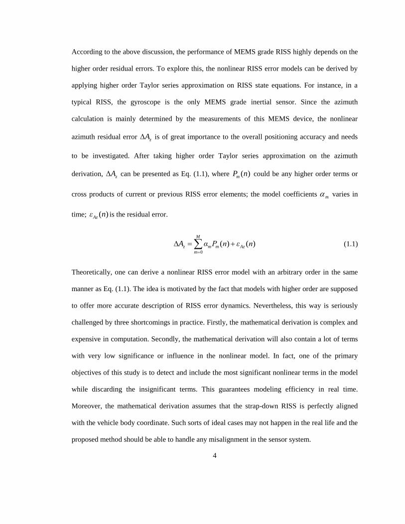
According to the above discussion, the performance of MEMS grade RISS highly depends on the

higher order residual errors. To explore this, the nonlinear RISS error models can be derived by

applying higher order Taylor series approximation on RISS state equations. For instance, in a

typical RISS, the gyroscope is the only MEMS grade inertial sensor. Since the azimuth

calculation is mainly determined by the measurements of this MEMS device, the nonlinear

azimuth residual error zA is of great importance to the overall positioning accuracy and needs

to be investigated. After taking higher order Taylor series approximation on the azimuth

derivation, zA can be presented as Eq. (1.1), where ( )mP n could be any higher order terms or

cross products of current or previous RISS error elements; the model coefficients m varies in

time; ( )Azε n is the residual error.

0

( ) ( )M

z m m Az

m

A α P n ε n

(1.1)

Theoretically, one can derive a nonlinear RISS error model with an arbitrary order in the same

manner as Eq. (1.1). The idea is motivated by the fact that models with higher order are supposed

to offer more accurate description of RISS error dynamics. Nevertheless, this way is seriously

challenged by three shortcomings in practice. Firstly, the mathematical derivation is complex and

expensive in computation. Secondly, the mathematical derivation will also contain a lot of terms

with very low significance or influence in the nonlinear model. In fact, one of the primary

objectives of this study is to detect and include the most significant nonlinear terms in the model

while discarding the insignificant terms. This guarantees modeling efficiency in real time.

Moreover, the mathematical derivation assumes that the strap-down RISS is perfectly aligned

with the vehicle body coordinate. Such sorts of ideal cases may not happen in the real life and the

proposed method should be able to handle any misalignment in the sensor system.

5

To conquer the above problems, the ultimate goal of this research is to find a numerical technique

for the modeling of nonlinear systems. The technique should provide the following advantages:

1. It can model RISS errors by detecting the most significant nonlinear error terms as well

as their weight coefficients.

2. During GPS availability, by accessing the knowledge of true RISS errors, it can adapt the

model structure to always best-fit the nonlinear RISS error online.

3. During GPS outages, the pre-built model is supposed to provide accurate predictions of

the nonlinear RISS errors.

4. The technique is able to tolerate the noisy MEMS sensor measurements corrupted by

non-stationary stochastic sensor errors.

5. It should maintain high computing efficiency so that the real-time positioning requests

can be satisfied.

This research also targets the embedded real-time realization of the proposed technique.

1.4 Research Contribution

This thesis is the very first one that suggests use of the Fast Orthogonal Search (FOS) algorithm,

an advanced nonlinear modeling technique, in fields of INS/GPS integration and, specifically, for

analysis of higher order inertial errors. It proves that FOS is very suitable for the accuracy

enhancement on multi-sensor integration as it does not require the system being modeled keeps

the same behavior between its modeling and prediction stages (this pre-condition is necessary for

many other nonlinear techniques). This research revealed the computing efficiency of the

proposed method as well. It discovered that FOS is more appropriate for error-model-based

system rather than working directly on global navigation states. The construction of KF/FOS

6

module also provided valuable experiences on how to select input parameters appropriately for

the creation of FOS candidates when applying this numerical technique in specific fields such as

the inertial error modeling for vehicle navigation. FOS is able to identify the system nonlinearity

using knowledge of system inputs and outputs even in a short term data window. It systematically

examines all the possible candidates involving higher order terms or cross products of system

inputs and outputs in a recursive scheme. Those candidates that minimize the model-fit mean

square error will be chosen at first to build the nonlinear model as the algorithm acknowledges

their obvious contribution to the system nonlinearity. This routine eventually achieves a precise,

yet still efficient polynomial that best-fits the target system. The pre-built model can then be used

to predict the nonlinear system behavior. Motivated by the above idea and the other estimating

structures like the neural network, an augmented KF/FOS module is proposed in this study. This

module keeps a Kalman filter working as usual to predict and correct linear INS errors.

Meanwhile, if GPS aiding signal exists, the true nonlinear INS errors can be derived and sent to

FOS together with linear INS error prediction from KF. These data are used to create candidates

by FOS in the background so that the algorithm builds and updates the nonlinear INS error model

online. Should GPS outage occur, the very last FOS model is supposed to best fit the local

nonlinear INS error. FOS model output can then be utilized with KF prediction to correct both the

linear and nonlinear INS errors.

The KF/FOS module is applied in MEMS grade RISS for both 2D and 3D vehicle navigation.

Several road tests are carried out to evaluate its effectiveness in the vehicle dynamics. The

experiment results prove that the proposed method outperforms the KF-only solution. Its average

enhancement on positioning accuracy during GPS outages is over 60% with respect to the results

of KF alone. In addition, the improvement is consistent throughout different road test trajectories

with various vehicle dynamics. All these reports show the great advantages of KF/FOS module

7

over KF-only on the overall navigation performance and reliability. To evaluate the computing

efficiency, a real-time implementation of KF/FOS module is deployed on a general purpose

digital signal processor. Testing results on the hardware platform show that KF/FOS module has

prompt responds to allow the online vehicle navigation.

In addition, a data logger is developed in this study to perform the front-end data acquisition. It

offers a standard interface to upload multi-sensor readings in the unified packets. This drastically

mitigates the overhead of the host system as there is no need for the host to deal with INS/GPS

data streaming details any more. Instead, the host can concentrate on running the data fusion

algorithm like the KF/FOS module. Obviously, the data logger is also a very good test-bench to

allow the evaluation of other multi-sensor integration techniques in the future.

1.5 Dissertation Outline

Chapter 2 reviews the concepts of inertial navigation system, global navigation satellite system

(GNSS), and their integration. Backgrounds like the navigation coordinate system are also

presented. Other multi-sensor solutions for vehicle navigation are discussed briefly in the

literature survey.

Chapter 3 details the principle of inertial navigation system (INS) and provides the analysis of

INS errors. After describing 3D INS structure and mechanism, this chapter discusses the sources

and characteristics of INS errors. A MEMS-based reduced inertial sensor system (RISS) is

reviewed afterwards for both 2D and 3D vehicle navigation. The chapter also gives the linear INS

error model and analyzes the significance of its nonlinear residual errors especially for the MEMS

system. In addition, Kalman filter (KF) and its application in INS/GPS integration are presented

by the end of this chapter. The limitations of KF and the other alternatives are covered as well.

8

In Chapter 4, a nonlinear modeling technique - Fast Orthogonal Search algorithm (FOS) is

reviewed. As a general purpose numerical approach, this method identifies system nonlinearity

and builds its model in a recursive scheme. The model can then accurately predict outputs of the

original system. In this study, FOS algorithm is proposed to model and compensate nonlinear

inertial errors.

Chapter 5 introduces KF/FOS module. The idea is to keep Kalman filter working on linear

inertial errors as usual and let the KF residual errors be handled by FOS algorithm. By removing

both linear and nonlinear error components, this augmented structure improves the navigation

accuracy. The application of KF/FOS module in both 2D and 3D cases is presented. Its

effectiveness is verified in several road tests. The experimental results are provided with analysis.

Chapter 6 presented the design of a front-end data logger. After describing the system

architecture, this chapter demonstrated how to synchronize multi-sensor measurements correctly.

A dedicated protocol was then developed to wrap all the sensor readings into unified packets.

Once received these packets, the host can extract INS/GPS information from them without

necessarily knowing the setup details of any front-end sensor. This reduces the workload of the

host and lets it focus on executing navigation algorithms. Experimental results are presented to

validate the logger behaviors. The effectiveness of KF/FOS module is reconfirmed on the road

test trajectory data recorded by the logger.

Chapter 7 proposed the real-time implementation of KF/FOS module for MEMS-based INS/GPS

integration on the hardware. It firstly defines the application objectives and then compares

different hardware platforms. Digital signal processor (DSP) is eventually selected to prototype

the design. Corresponding system architecture and setup are illustrated in detail. The road test

9

experimental results prove the consistency between the prototype design and the algorithm. They

validate the real-time performance of this hardware realization as well.

The conclusions are presented in Chapter 8. This chapter summarizes all the research work in this

thesis and provides suggestions for future study.

10

Chapter 2

Overview of Navigation Systems

According to the literatures [1][11], navigation has two fundamental missions in general. The first

one is to determine the position, velocity, and attitude of a target with respect to a known

reference in terms of monitoring observations. The second one is to provide guidance for this

target to reach the desired destination. Clearly, completion of the second mission relies on the

accuracy of the first one. In this study, the term navigation covers the first mission only. The

moving target to be monitored is also narrowed to land vehicles. Then, the vehicle navigation

here refers to the procedure of determining automotive navigation states including the position,

velocity, and attitude. In the following chapters, this concept is rephrased as vehicle positioning

when only the position is required.

2.1 Categories of Navigation Approaches

Many literatures [1][3][5][8][9][11] had discussed the categories of navigation approaches from

different point of views. They agreed in common that all these strategies can be classified into

two major types according to their mechanism: Dead Reckoning (DR) and Reference-based

absolute solutions.

2.1.1 Dead Reckoning Systems

Dead Reckoning (DR) derives the vehicle position from the knowledge of the previous position

and the measurement of vehicle dynamics over the elapsed time [5][9][12]. Essentially, it is a

recursive process of calculating the present navigation states in terms of their early values by

taking the state changes during this period into consideration.

11

All information required by DR operations is restrained in the outputs of DR device itself. This

ensures DR platforms as self-contained modules that are immune to possible external interference.

They guarantee continuous navigation results as well since almost all DR devices offer their

measurements at certain data rate in all conditions. Due to the fact DR calculates its updates

solely from previous value, any errors throughout the process will accumulate. Without external

correction, the error grows over time and become the major disadvantage of DR solutions.

At present, the inertial navigation system (INS) and the odometry are the most popular DR

solutions. Both are widely utilized in vehicle navigation.

(1) Inertial Navigation System

A typical inertial navigation system (INS) consists of a measuring module and a data acquisition

unit. Accelerometers and gyroscopes are installed in the measuring module to measure the linear

acceleration and the angular velocity along their sensing axes, respectively. Their analog outputs

reflecting the physical measurements are passed to the data acquisition unit for signal

conditioning. The latter usually contains analog-to-digital converters (ADC) or a microcontroller

with built-in ADC, which bring the inertial measurements into the digital world. The entire

platform is also called inertial measurement unit or IMU. Given the acceleration and angular

velocity from IMU, it is easy to compute the changes of velocity V , direction angle ,

and position P over time t according to kinematics. E.g. V dt , dt ,

2P dt . The above formula proved that INS is an independent system as it only relies on

its own measurement to offer navigation service. However, inertial sensor bias and drift result in

accumulative error growth over time in the integrations. This undermines the overall performance

of INS and, thus, INS alone is inadequate to maintain the accuracy of long term navigation.

12

(2) Odometry

Odometry is very suitable for wheel-based moving platforms. The vehicle odometer tells the

distance the vehicle has traveled from a starting location by measuring how far the wheels have

rotated [2]. This distance can be easily derived if given the circumference of the wheels. The

emerging of rotary encoders allows sensing the speed in an odometry style as well. They monitor

dynamics of the shaft including revolutions per minute (RPM) or the more precise angular

velocity at high sampling rates. RPM or the angular velocity can then be translated to speed value

by computing their product with the wheel circumference. This actually explains how the vehicle

speedometer works. It is inexpensive to collect odometry results as the shaft encoder and the

speedometer have become the built-in devices of autonomous robotics with wheels and the

vehicles, respectively. Moreover, almost all mainstream microcontrollers contain the pulse or

quadratic encoder interface as a standard peripheral, which enables seamlessly streaming of the

encoder data into the processing unit. As a DR solution, odometry still suffers from its error

growth over time. For instance, its distance error increases in proportion to the moving duration

without boundary and, thus, causes performance deterioration in the long term. Also, odometry

alone usually cannot provide a complete and accurate navigation solution as it is in lack of more

precise heading information.

2.1.2 Reference-based Absolute Solutions

Reference-based absolute solution refers to the navigation approaches that require measurements

with respect to known external reference or patterns. Unlike DR systems, methods in this type do

not evolve current navigation state from the previous one. They provide absolute positioning with

respect to a reference frame. Since no memory effects exist, the errors of these systems do not

accumulate and are always bounded in limits. This gives reference-based solutions advantages on

13

long term navigation accuracy. However, their overall performance is highly influenced by

possible external interference or/and signal loss that jeopardize their accuracy. Moreover, unlike

autonomous systems, most reference-based solutions have lower sampling rate, which leads to

their weakness in short term positioning accuracy.

(1) Global Navigation Satellite System

Global Navigation Satellite System (GNSS) is built by artificial satellite constellation

surrounding the Earth [1]. Its ground stations control every satellite to travel on the pre-defined

orbit so that the satellites work as positioning reference nodes and at least four of them are visible

anywhere on the Earth. They broadcast encoded radio frequency signals, which contain the

information of their current location. The ground receiver can decode this information and use it

together with the travel time of the same signal to determine the receiver's position [3]. According

to trilateration principle discussed later in section 2.3, the receiver's location on the Earth can be

obtained if knowing its distance to three satellites. In the real life, signals from a fourth satellite

are needed to synchronize the receiver clock. If no obstacles exist, GNSS signal is ubiquitous in

its satellite coverage. This makes GNSS very popular in absolute localization. Its performance is

also attractive as the positioning error is bounded to meters in case of good signal qualities [3]. At

present, GNSS is mainly challenged by possible signal interference and blockage during the radio

propagation and receiving.

(2) Compass

Driven by the Earth magnetic field, the compass needle always aligns itself pointing to the Earth

magnetic poles. This keeps the reference frame of magnetic compasses fixed to the Earth.

Therefore, compasses can tell the absolute heading angle from the North. Since heading angle has

fundamental influence on the navigation state, compasses are widely utilized to determine vehicle

14

orientations or assist the heading correction of accumulative Dead Reckoning error [2]. Their

performance degrades when the Earth magnetic field is distorted near power systems, steel

structure, and the other strong electromagnetic environments.

(3) Altimetry

Altimetry means using instruments like altimeters to measure the target's altitude compared to a

fixed level. Its general concept covers the underwater depth measurements as well. The

submarine depth gauge is a typical example. For land vehicles, the barometry altimeters are more

popular. Its mechanism is related to the fact that the atmospheric pressure decreases when the

altitude ascends. The varying density distribution of the atmosphere causes the nonlinearity

between the pressure and the altitude. Temperature changes make this relation more complicated.

Thus, barometers need sophisticated calibration to indicate the absolute altitude of targets

precisely.

(4) Map Matching

Map matching is defined as the process of correlating two sets of geographical positioning

information [11]. A common example is GNSS records of object position versus the digital map.

This method collects and analyzes absolute spatial information from different data sources to

generate more accurate positioning results via a matching operation. It is suitable for land

vehicles as they usually travel along the road networks labeled in maps. However, the availability

of map matching is limited in the mapped areas. Furthermore, it is relatively expensive to

maintain massive reference memory such as GIS databases for this approach.

15

(5) Other Emerging Techniques

With the advancing of wireless technology, wireless positioning systems other than GNSS are

recently introduced in navigation industry. They depend on WiFi, radio frequency identification

(RFID), or more general wireless local area networks (WLAN) to obtain positioning reference.

The above methods have limited success in land vehicle navigation as they are more appropriate

for in-door positioning. Other techniques like cellular networks, camera-based vision systems,

and light detection and ranging (LIDAR) are more practical for automobile applications.

However, their utilization is also restricted by the cost, computing complexity, and other

environmental impacts.

Nowadays, the trend is to combine different methods from both DR and absolute solutions. Their

mixture is supposed to overcome the drawbacks of each one alone and promises better

performance. Among these various combinations, the integration between GNSS and INS is more

popular because of its advantages on the navigation accuracy, reliability, system cost, portability

to vehicles, and so forth. The rest of this chapter will hereby cover the background related to INS,

GNSS, and their integration.

2.2 Inertial Navigation System

2.2.1 Principle of Inertial Navigation

Inertial navigation system is a self-contained navigation module in which measurements provided

by inertial sensors are used to track the position and orientation of a moving platform related to

the known initial position, orientation, and velocity [12]. According to classical mechanics,

inertia is an inherent property of any objects to maintain constant translational and rotational

motion. A change of motion occurs as a result of forces or torques being applied to overcome the

object's inertia [13]. Newton's second law describes this relation quantitatively as shown in Eq.

16

(2.1), where F refers to the force, m denotes the object's inertial mass, a means the acceleration

(time derivative of velocity V).

F m a mdV

dt (2.1)

Accelerometers, for example, rely on Eq. (2.1) to translate the force measurement into their

motion dynamic readings. While accelerometers monitor linear acceleration by measuring the

force along the same direction, gyroscopes derive rotation rates from their measurements of the

centripetal force. The acceleration and rotation rate can then be used in the first and second order

integrals to determine the object’s velocity, position, and orientation, respectively.

According to the above introduction, inertial sensors are the elementary devices for any INS.

Since the dawn of inertial sensing in the early 1920s, mechanical inertial sensors have dominated

the applications of standalone guidance, navigation, and control [14]. However, in late 1980s, this

dominance was challenged by new technologies like Ring Laser Gyro (RLG) and Fiber Optical

Gyro (FOG). Recently, with the rapid booming of micro-electro-mechanical-system (MEMS),

MEMS-based inertial sensors have introduced major change in INS. They are able to monitor

acceleration and rotation rates with low life cycle cost, small size, low production cost, low power

consumption, and large volume manufacturing [15]. At present, over half of the tactical and

commercial grade inertial sensing market has been occupied by MEMS-based sensors.

Almost all MEMS devices are made from silicon wafer, similar to conventional integrated

circuits [17]. This allows the seamless integration of inertial sensing mechanical structure and

peripheral interfaces (ADC, calibration electrical circuits, etc.) in one package or even on the

same silicon wafer. Specifically, as shown in Fig. 2-1, MEMS gyros are designed to measure

displacement of structure (representing rotation) caused by Coriolis force in a capacitive silicon /

17

piezoelectric quartz instrument. Similarly, the physical mechanisms underlying MEMS

accelerometers include capacitive, piezo-resistive, electromagnetic, piezoelectric, ferroelectric,

optical and tunneling [18]. The most popular type is based on capacitive transduction, although,

in which there exists a nonlinear capacitance versus displacement characteristic. In ideal cases,

the displacement or torque of inertial sensing structure should be proportional to the input

acceleration or Coriolis force. Possible nonlinear distortion of MEMS sensing structure violates

this rule. It inherently causes the instability and intensive nonlinearity in the errors of MEMS-

based INS.

Fig. 2-1: Capacitance sensing structure (comb fingers) of InvenSense gyro IDG – 300 [16]

2.2.2 Introduction of Reference Frames

As strap-down modules, inertial sensors are mounted directly onto the moving platform. Fig. 2-2

illustrates its arrangement details. By aligning three gyroscopes and three accelerometers on three

mutually orthogonal axes X, Y, and Z, both the rotational and translational motions can be

monitored along the three axes [19]. Since the sensors are fixed onto the target, coordinates X-Y-

Z, which represents reference frame of the sensor measurements, is always rigidly attached to the

18

moving platform [20] and aligned to the local transverse, forward, and vertical directions. This

coordinates system is called body level frame (BLF).

X

Y

Z

z

x

y

zf

xf

yf

(a)

Fig. 2-2: Structure of body level frame

Although sensor measurements in BLF describe the straightforward motion dynamics, they

cannot directly tell the target's geodetic information that is of more importance for vehicle

positioning. To solve this problem, instead of BLF, a local level frame (LLF) is preferred as the

coordinate system to express vehicle’s position on the Earth. Being aligned to local North, East,

and vertical directions, LLF has advantages when representing the direct geodetic information.

Fig. 2-3 depicts its structure.

f – Acceleration ω – Rotation rate

19

: :

:h

Latitude Longitude

Altitude

eY

eZ

eX

eN

E

UP

h

Equator

Greenwich

(b)

Fig. 2-3: Structure of local level frame

When focusing on land vehicle navigation, BLF and LLF are most frequently used. Inertial

sensors output their measurements in BLF. Meanwhile, the positioning results are expressed in

LLF. Due to the above reasons, the INS inputs and outputs discussed in this thesis are restrained

in BLF and LLF, respectively. In fact, the primary task of INS is to transfer the BLF inputs into

the LLF outputs. More details about mapping from BLF to LLF are discussed in Chapter 3. The

LLF is used in this study for two main reasons. The first is that the three attitude angles (pitch,

roll, and azimuth) can be directly obtained at the output of the LLF mechanization. The second

reason is the fact that the errors in the navigation parameters along the horizontal plane are

bounded due to the Schuler effect [9].

2.2.3 Overview of INS errors

INS is highly affected by inertial sensor errors, misalignment, and error propagation. The inertial

sensor error mainly consists of sensor bias, scale factor errors, and random noise [4]. For those of

deterministic errors such as bias offset and scale factor, a standard calibration procedure can be

used to obtain them through simple laboratory experiments. On the other hand, stochastic errors

meridian

20

include the bias drift, scale factor instability, white noise, random walk, thermal noise, 1/f noise,

and interference between internal electromechanical devices [5]. Due to their random nature,

stochastic sensor errors are difficult to be fully corrected. Instead, error modeling is more

practical to allow estimating and compensating for their effects. In addition, the imperfection of

sensor mounting may result in non-orthogonality of the axes defining the body level frame. This

will further degrade the accuracy of navigation results in the local level frame. The effects of non-

orthogonality or misalignment can be avoided using lab experiments as well. More details about

linear inertial sensor errors can be found in Chapter 3.

In case of MEMS sensors, due to their inherent error characteristics discussed before,

conventional linear error modeling and prediction techniques may not be adequate to preserve

measuring accuracy. Higher order residual errors propagate via the mapping of reference frames.

Without external correction, they accumulate over time throughout the whole vehicle traveling

trajectory, thus severely jeopardizing the overall positioning performance. This is why more

sophisticated modeling of stochastic and nonlinear residual errors is so important and crucial for

MEMS-based INS.

2.3 GNSS Solution

2.3.1 Overview of Existing GNSS

Since 1970s, satellite-based navigation systems emerged firstly for the military purpose. They

entered the civilian market afterwards and soon became very successful in autonomous

positioning. Today, owing to its global service coverage and positioning quality, GNSS has

become a dominant technique for land vehicle positioning. So far, there are only two fully

operational GNSS: GPS from the United States and GLONASS from Russia.

21

GPS was developed by the United States Department of Defense. It has been operational since

1978 and globally available since 1994 [21]. GPS is currently the world's most widely utilized

GNSS. As a dual-use system, it has fulfilled numerous positioning requirements in both civil and

military fields since 1990s.

GLONASS (GLObal NAvigation Satellite System) is another GNSS operated by the Russian

Space Forces [22]. Its fully functional constellation was completed in 1995. However,

GLONASS was then in trouble of disrepair, thus causing coverage leakages and frequent service

interruptions [22]. In early 2000s, Russia started to restore the global availability of GLONASS.

It is now open to civilian applications as well.

Other GNSS alternatives are still in development. Chinese regional satellite-based navigation

system is evolving into the global Compass navigation system by 2020 [23]. The European

Union's Galileo positioning system is still in the initial deployment phase. Its fully operation is

expected to be achieved by 2020 at the earliest [24].

Since GPS is currently the most popular globally covered and fully operational system, all the

discussion below will focus on it as the major GNSS example.

2.3.2 Positioning Mechanism of GPS

The fully operational GPS includes 24 or more (currently 31) active satellites. There are four or

more satellites uniformly dispersed on each one of the six orbits [21][22]. The orbits are inclined

at an angle of 55◦ relative to the equator and are separated from each other by multiples of 60

◦

right ascension [3]. This constellation geometry makes four or more GPS satellites visible

anywhere on the Earth. GPS utilizes the concept of time of arrival ranging to determine user

position, which entails measuring the time it takes for a signal from a known location (satellite

coordinates) to reach a user receiver [22][25].

22

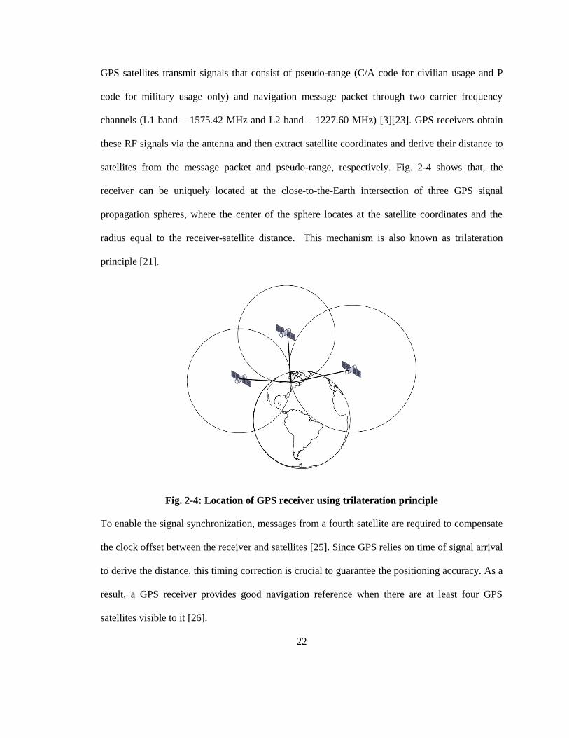
GPS satellites transmit signals that consist of pseudo-range (C/A code for civilian usage and P

code for military usage only) and navigation message packet through two carrier frequency

channels (L1 band – 1575.42 MHz and L2 band – 1227.60 MHz) [3][23]. GPS receivers obtain

these RF signals via the antenna and then extract satellite coordinates and derive their distance to

satellites from the message packet and pseudo-range, respectively. Fig. 2-4 shows that, the

receiver can be uniquely located at the close-to-the-Earth intersection of three GPS signal

propagation spheres, where the center of the sphere locates at the satellite coordinates and the

radius equal to the receiver-satellite distance. This mechanism is also known as trilateration

principle [21].

Fig. 2-4: Location of GPS receiver using trilateration principle

To enable the signal synchronization, messages from a fourth satellite are required to compensate

the clock offset between the receiver and satellites [25]. Since GPS relies on time of signal arrival

to derive the distance, this timing correction is crucial to guarantee the positioning accuracy. As a

result, a GPS receiver provides good navigation reference when there are at least four GPS

satellites visible to it [26].

23

2.3.3 GPS Signal Characteristics

All radio-based systems suffer from the possible RF signal blockage. Other than that, GNSS

signal attenuates in transmission. Negative effects like the interference, signal blockage, and the

multipath propagation jeopardize the signal quality in the meantime. For instance, in GPS-denied

environments such as urban canyons, tunnels, and forests, GPS service may be unreliable or

totally lost. The gaps of GPS unavailability are also called GPS outages.

The path losses of GPS signal strength depend on both the distance of travel and the transmitting

medium. The latter is more important as the distance dependent loss can be well modeled if the

transmitting medium is homogeneous [27][28][29]. GPS signal encounters three different

mediums: vacuum, ionosphere, and troposphere. Ionosphere refers to the Earth atmosphere layer

stretching from a height of about 50 km to more than 1000 km above the sea level. It has massive

electrons and positive charged ions formed by the ionizing force of the sun [27]. Troposphere is

the lowest atmosphere layer with an average depth up to 17 km. It contains over 80% atmosphere

mass and almost all its water vapor and aerosols [28]. GPS signal was mainly weaken in these

two atmosphere layers. A typical attenuation is 0.035 dB at the zenith and increases by a factor of

10 at low elevation [26]. GPS signals reach the Earth with a power level at -130 dBw in the

optimal cases. Currently, advanced GPS receiver is capable of demodulating L1 band signals with

power levels at -160 dBw [28]. High sensitivity GPS antennas with low noise amplifiers (LNA)

help these receivers to extract GPS band signals buried in noisy background [29]. They reduce

effects like the thermal noise introduced by ions and vapors in atmosphere to restore the signal-

to-noise ratio. Consequently, GPS receivers can work in areas with lower signal strength or a

faster Time-To-First-Fix (TTFF) from the cold start can be obtained.

To further improve the performance, the dual frequency receivers are used to demodulate carrier

signals at multiple frequencies [26]. They excel on compensating signal propagation delays

24

caused by the refraction of RF waves in the ionosphere [29]. Since the radio signals are slowed

down inversely proportional to the square of their frequency while passing the ionosphere, the

measuring of signal latencies at different bands will benefit the analysis and correction of

ionospheric errors.

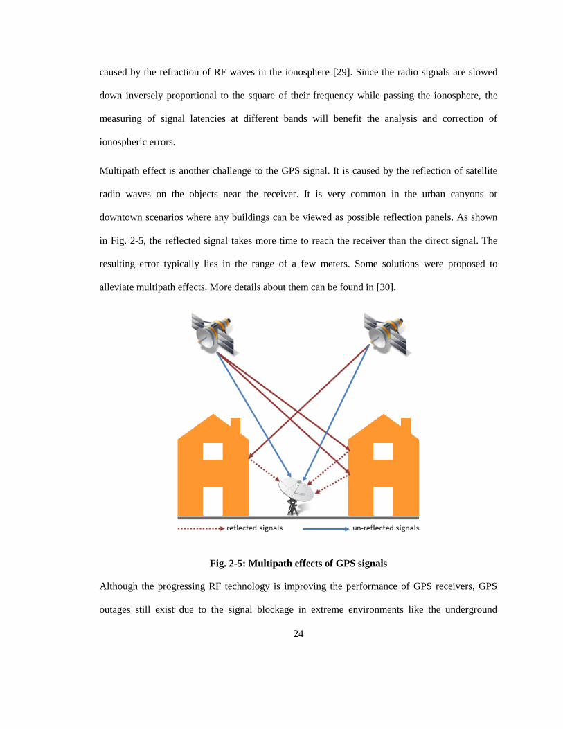
Multipath effect is another challenge to the GPS signal. It is caused by the reflection of satellite

radio waves on the objects near the receiver. It is very common in the urban canyons or

downtown scenarios where any buildings can be viewed as possible reflection panels. As shown

in Fig. 2-5, the reflected signal takes more time to reach the receiver than the direct signal. The

resulting error typically lies in the range of a few meters. Some solutions were proposed to

alleviate multipath effects. More details about them can be found in [30].

Fig. 2-5: Multipath effects of GPS signals

Although the progressing RF technology is improving the performance of GPS receivers, GPS

outages still exist due to the signal blockage in extreme environments like the underground

25

parking lot or the signal deterioration in streets surrounded by skyscrapers. To bridge the GPS

gaps in these challenging areas, research efforts begin to focus on augmenting GPS with other

techniques [22][23][31][32][33]. Most of the current solutions derive from two basic ideas: GPS

signal relay or introducing complementary systems. Typical examples of GPS signal relay are the

Satellite-based and Ground-based Augmentation Systems (SBAS and GBAS) [22]. They depend

on broadcast relay stations like the extra geo-stationary satellites or terrestrial radio towers to

deliver the amplified GPS signal to their uncovered areas [23]. A similar idea is to augment GPS

by other GNSS like GLONASS to enlarge the signal coverage. Nevertheless, all these methods

still fail in the extreme environments that are totally isolated to external RF signals. To conquer

the above problem, recent research suggests integrating GPS with its complementary systems.

Possible candidates include local wireless-based positioning systems (e.g. WLAN, RFID, WiFi,

etc.) and Dead Reckoning sensors. The local wireless systems rely on reference nodes pre-

installed in specific areas [31]. Hence, it is more suitable for in-door positioning. In contrast, DR

sensors do not have this restriction and, thus, are more appropriate for vehicle positioning [32].

So far, combination of GPS and DR sensors (e.g. INS/GPS integration) has become a primary

multi-sensor approach for vehicle navigation [33] and is also the focus of this research.

2.4 INS/GPS Integration

2.4.1 Benefits of INS/GPS Integration

In order to overcome the disadvantages associated with the standalone GPS and INS, the two

systems often cooperate with each other in a complimentary fashion so that their integration has

superior performance in comparison with either a GPS or an INS alone [34].

As mentioned in Section 1.2, INS offers short-term navigation accuracy. The data rate of its

measurement is much higher than GPS updates. As an independent module, INS always outputs

26

continuous navigation results no matter GPS signals exist or not. However, due to the inherent

features, INS suffers from its growing errors without boundaries over time. Hence, it requires

aiding reference such as GPS signals to correct the errors in computing navigation parameters and

allow the online calibration of long-term sensor drift. Moreover, GPS reference also help to

perform the online alignment and state estimation of INS platform, which, in turn, help to slow

down the INS error growth in GPS outages.

Compared to INS, GPS has the advantages of keeping bounded navigation accuracy in the long

term. For instance, GPS-derived positions have approximately white noise characteristics over the

whole frequency range [34]. Therefore, appropriate error modeling can be applied to enhance

GPS performance so that its information becomes accurate enough as reliable aiding reference for

the long term navigation [35]. However, this is not the case for the vehicle at all the time since

GPS signals may be lost when driving around obstacles (downtown area, tunnels, highways, tree

lined streets, etc.), or with undesired weather conditions [1][36]. The satellite signal blockage

(jamming, interference, multi-path effects, etc.) could result in deterioration of the overall

positioning accuracy. Also, relatively low GPS sampling rate may not satisfy the short term

accuracy, which requires high-bandwidth / high-speed angular rate and acceleration information.

On the other hand, since INS applies independent measuring, it is immune to external disturbance

[37] and is able to feedback short term motion dynamics continuously in real-time. Moreover,

INS can provide accurate position and velocity data for GPS signal acquisition and reacquisition

after outages. This reduces the time and the search domain required for the detection of GPS

signals [38].

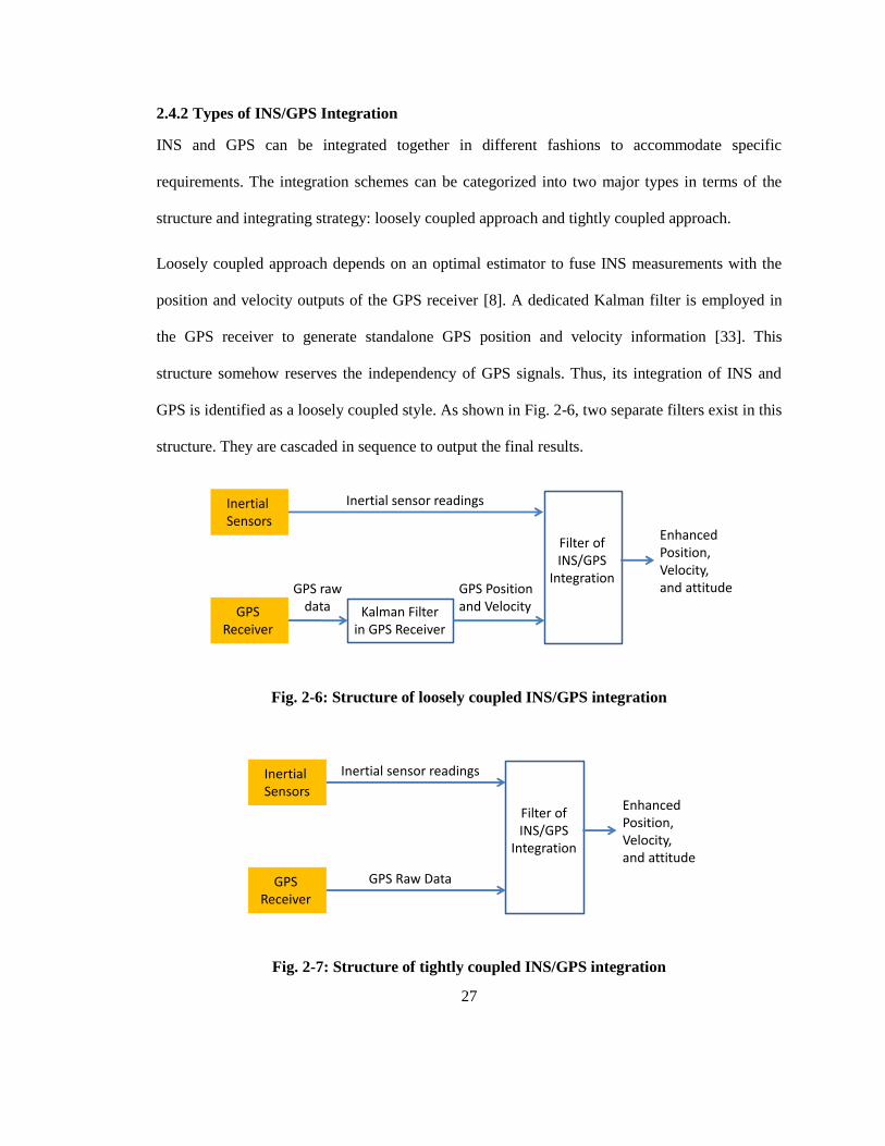
27

2.4.2 Types of INS/GPS Integration

INS and GPS can be integrated together in different fashions to accommodate specific

requirements. The integration schemes can be categorized into two major types in terms of the

structure and integrating strategy: loosely coupled approach and tightly coupled approach.

Loosely coupled approach depends on an optimal estimator to fuse INS measurements with the

position and velocity outputs of the GPS receiver [8]. A dedicated Kalman filter is employed in

the GPS receiver to generate standalone GPS position and velocity information [33]. This

structure somehow reserves the independency of GPS signals. Thus, its integration of INS and

GPS is identified as a loosely coupled style. As shown in Fig. 2-6, two separate filters exist in this

structure. They are cascaded in sequence to output the final results.

Inertial Sensors

GPSReceiver

Kalman Filterin GPS Receiver

Filter ofINS/GPS

Integration

Inertial sensor readings

GPS rawdata

GPS Positionand Velocity

EnhancedPosition, Velocity,and attitude

Fig. 2-6: Structure of loosely coupled INS/GPS integration

Inertial Sensors

GPSReceiver

Filter ofINS/GPS

Integration

Inertial sensor readings

EnhancedPosition, Velocity,and attitude

GPS Raw Data

Fig. 2-7: Structure of tightly coupled INS/GPS integration

28

Tightly coupled approach relies on estimation techniques to fuse INS measurements with GPS

raw data. It synthesizes the raw GPS messages like the pseudo-ranges and IMU readings in the

same filter to determine the target's position, velocity, and attitude [33]. As shown in Fig. 2-7,

tightly coupled structure has only one centralized filter, which integrates INS and GPS at the raw

data level.

Loosely coupled approach requires signals from at least four GPS satellites to supply accurate

GPS position and velocity for the integration [25]. Tightly coupled approach breaks through this

limitation as it offers GPS readings even if only one satellite is visible [8][33]. This advantage

intensifies the robustness of INS/GPS integration when most GPS signals are blocked by

obstacles that are very common throughout a travel in the downtown scenario. In addition, since

tightly coupled approach works on GPS raw data directly, it can distinguish the signal quality of

different GPS satellites [39]. This allows to extract healthy GPS information and to reject the

poor signals sent by satellites with low elevation. In general, tightly coupled approach provides

better performance than loosely coupled approach. The cost of this enhancement is the extra work

to implement the more sophisticated integration filter.

The filter of INS/GPS integration can predict either navigation states directly or navigation error

states instead. If using the error state filter, its output contains the error prediction of position,

velocity, and attitude in the un-aided INS results [8]. The navigation state estimation can then be

obtained by compensating the un-aided INS results with the above error predictions. This

procedure repeats in the vehicle travel to achieve the online INS/GPS integration [32]. Since INS

computes current navigation state according to the previous one, the enhanced navigation state

from the integration filter can be fed back to the INS computation and improve its performance.

This working scheme is also known as the closed-loop INS/GPS integration [33][34]. On the

29

other hand, there exist no navigation state feedbacks in the open-loop INS/GPS integration. In the

scope of this thesis, research efforts mainly focus on the open-loop loosely coupled INS/GPS

integration.

2.4.3 Methodologies of INS/GPS Data Fusion

The INS/GPS data fusion is commonly performed using Kalman filter (KF) [40][41][42]. KF-

based integration technique requires dynamic models of both INS and GPS state errors, a

stochastic model of inertial sensor errors, and covariance matrices (a priori information) of the

data provided by both systems [40]. Due to its consistent long term accuracy, GPS reference is

used to update the KF predictions of INS state errors. These corrected error prediction can then be

utilized to prevent the long term error growth of INS. Meanwhile, the accurate short term

information provided by INS can be used to bridge GPS outages [35]. Should a GPS outage occur,

KF operates in prediction mode, correcting INS results according to the system error models

mentioned before.

KF shows adequate performance when integrating GPS with tactical or navigational grade INS

[43]. The reason lies in the fact that the linear model used by KF can describe the error

characteristics of those high-end INS accurately. However, the goal to maintain reasonable cost

level is driving the need to develop much lower cost MEMS inertial sensors and their integration

with GPS. Currently, the idea is mainly challenged by the complexity of MEMS sensor errors. As

mentioned in Section 2.2, measurements of MEMS grade inertial sensors are contaminated by

massive nonlinear errors and non-stationary stochastic noise, which cannot be accurately

described by linear error models. This undermines the effectiveness of KF prediction and makes

KF-based integration inappropriate for MEMS grade devices [10].

30

To overcome KF limitations, nonlinear techniques such as artificial intelligence (AI) were

introduced to handle INS errors with intensive nonlinearity [34][36][44][45]. By learning local

error statistics, AI-based methods adjust the parameters in a fixed nonlinear structure to imitate

the behavior of nonlinear INS errors [36]. During GPS outages, the trained AI structure output the

prediction of nonlinear INS errors to compensate for their effects. As a result, AI-based methods

enhance the reliability of MEMS grade INS/GPS integration. The effectiveness of AI approaches

highly depends on the consistency of error behaviors in the training stage and prediction stage

[44]. This means that AI results can be poor in circumstances where the statistics of nonlinear

INS errors change greatly between the two stages. Another major challenge related to AI-based

methods is their computational complexity during the training procedure that prevents them from

being used in real-time [45][46]. The limitation of AI-based methods motivates the desire of other

nonlinear solutions with better robustness.

More details about KF-based INS/GPS integration and its AI-based alternatives are discussed in

Chapter 3. To provide better performance over these methods, a nonlinear modeling technique is

proposed in Chapters 4 and 5.

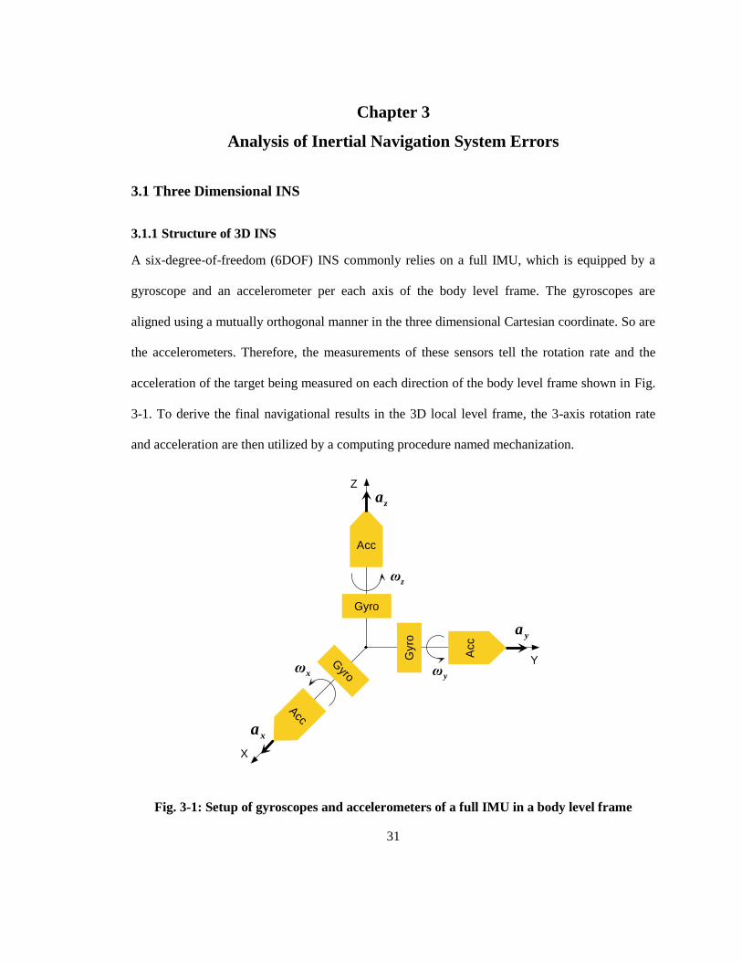
31

Chapter 3

Analysis of Inertial Navigation System Errors

3.1 Three Dimensional INS

3.1.1 Structure of 3D INS

A six-degree-of-freedom (6DOF) INS commonly relies on a full IMU, which is equipped by a

gyroscope and an accelerometer per each axis of the body level frame. The gyroscopes are

aligned using a mutually orthogonal manner in the three dimensional Cartesian coordinate. So are

the accelerometers. Therefore, the measurements of these sensors tell the rotation rate and the

acceleration of the target being measured on each direction of the body level frame shown in Fig.

3-1. To derive the final navigational results in the 3D local level frame, the 3-axis rotation rate

and acceleration are then utilized by a computing procedure named mechanization.

Gyro

Gyro

Gyro

Acc

Acc

Acc

xω yω

zω

xa

ya

za

X

Y

Z

Fig. 3-1: Setup of gyroscopes and accelerometers of a full IMU in a body level frame

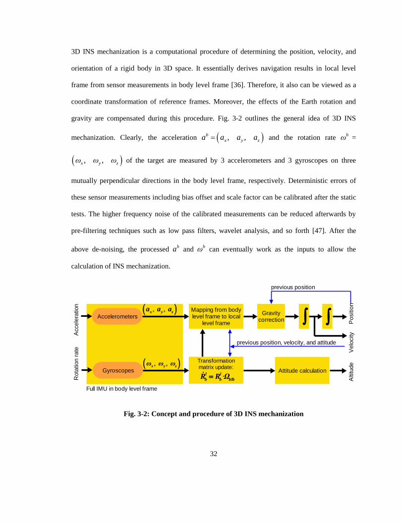
32

3D INS mechanization is a computational procedure of determining the position, velocity, and

orientation of a rigid body in 3D space. It essentially derives navigation results in local level

frame from sensor measurements in body level frame [36]. Therefore, it also can be viewed as a

coordinate transformation of reference frames. Moreover, the effects of the Earth rotation and

gravity are compensated during this procedure. Fig. 3-2 outlines the general idea of 3D INS

mechanization. Clearly, the acceleration , ,b

x y za aa a and the rotation rate bω =

, ,x y zω ω ω of the target are measured by 3 accelerometers and 3 gyroscopes on three

mutually perpendicular directions in the body level frame, respectively. Deterministic errors of

these sensor measurements including bias offset and scale factor can be calibrated after the static

tests. The higher frequency noise of the calibrated measurements can be reduced afterwards by

pre-filtering techniques such as low pass filters, wavelet analysis, and so forth [47]. After the

above de-noising, the processed ba and

bω can eventually work as the inputs to allow the

calculation of INS mechanization.

Mapping from bodylevel frame to local

level frame

Transformationmatrix update:

·l l

b b blbRR Ω

Gravitycorrection

Attitude calculation

Accele

ration

Ro

tation

rate

Accelerometers

Gyroscopes

, ,x y z

a a a

, ,x y zω ω ω

Full IMU in body level frame

Po

sitio

nV

elo

city

Altitude

previous position, velocity, and attitude

previous position

Fig. 3-2: Concept and procedure of 3D INS mechanization

33

3.1.2 Equations of 3D INS Mechanization

(1) Position mechanization equations

The latitude, longitude, and altitude of a moving object can be obtained from its velocities along

the East, North, and vertical directions as follows [10]:

1

0 0

0 0

0 0 1

1

1·

( )cos

e

n l

u

R h

λ VR

V

r V D

hh

V

(3.1)

Vector , ,T

r hλ represents latitude, longitude, and altitude of the object’s local position.

R is the radius of the Earth and vector , ,T

l e n uV V V V denotes velocity of the object along

the East, North, and vertical directions in the local level frame.

(2) Velocity mechanization equations

According to geometry knowledge, the transformation matrix (l

bR ) between the body level frame

and the local level frame can be presented as follows [10]:

cos cos sin sin sin sin cos cos sin sin sin cos

sin cos cos sin sin cos cos sin sin cos sin cos

cos sin sin cos cos

z z z z z

l

b z z z z z

A r A p r A p A r A p r

A r A p r A p A r A p r

p r p p r

R

(3.2)

zA , p , and r represent the azimuth, pitch, and roll of the object, respectively, in the body level

frame. The measurements of acceleration , ,T

b x y za a aa in body level frame can be

converted to local level frame using the rotation matrix l

bR in Eq. (3.3), where vector

34

, ,T

l e n ua a aa denotes the acceleration of the object along the East, North, and vertical

directions in the local level frame. By taking the effects of the Earth’s rotation, the change of

orientation in local level frame with respect to the Earth, and the Earth’s gravity field into

consideration, the velocity mechanization equation can be obtained as Eq. (3.4).

·

e x

l l

l n b b b y

u z

a a

a R a aa R

a a

(3.3)

2 ·( )l l l

l b b ie el l lV R a V g (3.4)

0, 0,T

lg g represents the gravity vector. l

ie and l

el are the skew-symmetric

matrices corresponding to l

ie and l

el , respectively. Specifically, l

ie denotes the rotation

between inertial frame and the Earth-Centered-Earth-Fixed (ECEF) frame; l

el denotes the

rotation between the ECEF frame and local level frame. Both of them are measured in the local

level frame and expressed by Eq. (3.5) [48], where e is the rotation rate of the Earth (15.04◦/h).

tan0

0 sin costan

sin 0 0 , 0

cos 0 0

0

e e

e e

l l e nie e el

ee n

R

V V

R hω ωV V

ωR h R h

ωV V

R

h

h R h

(3.5)

(3) Attitude mechanization equations

According to Eq. (3.2), the attitude (azimuth, pitch, and roll) can be obtained by using

trigonometric relations of elements in matrix l

bR . Also, they can be updated concurrently through

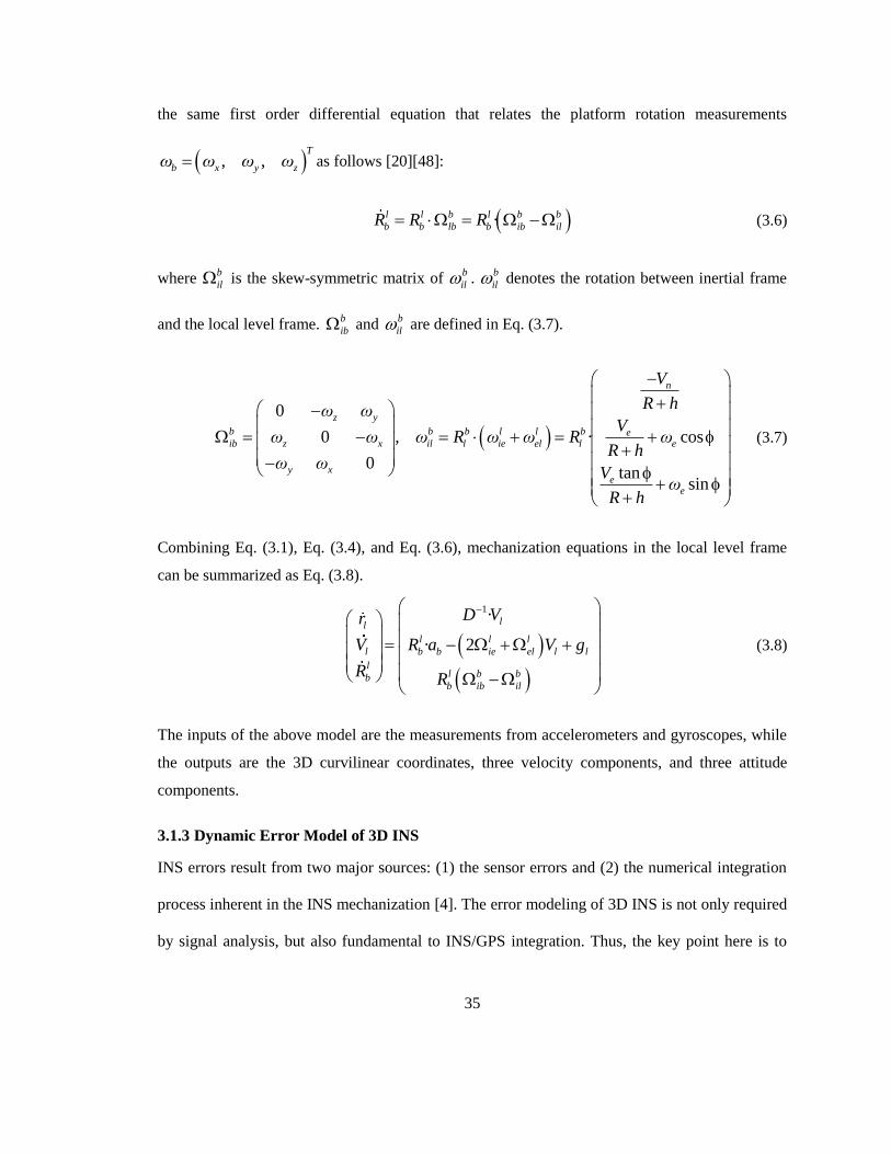
35

the same first order differential equation that relates the platform rotation measurements

, ,T

b x y zω ω ω ω as follows [20][48]:

·l l b l b b

b b lb b ib ilR R R (3.6)

where b

il is the skew-symmetric matrix of b

il . b

il denotes the rotation between inertial frame

and the local level frame. b

ib and b

il are defined in Eq. (3.7).

· co

0

0 s

tansin

,

0

n

z y

b b b l l b eib z x il l ie el l e

y xe

e

V

R hω ωV

ω ω ω R ω ω R ωR h

ω ωV

ωR h

(3.7)

Combining Eq. (3.1), Eq. (3.4), and Eq. (3.6), mechanization equations in the local level frame

can be summarized as Eq. (3.8).

1

2

·

·

ll

l l l

l b b ie el l l

ll b bbb ib il

Dr

Va

R

V

V R g

R

(3.8)

The inputs of the above model are the measurements from accelerometers and gyroscopes, while

the outputs are the 3D curvilinear coordinates, three velocity components, and three attitude

components.

3.1.3 Dynamic Error Model of 3D INS

INS errors result from two major sources: (1) the sensor errors and (2) the numerical integration

process inherent in the INS mechanization [4]. The error modeling of 3D INS is not only required

by signal analysis, but also fundamental to INS/GPS integration. Thus, the key point here is to

36

construct appropriate INS error model, which takes into consideration both the inertial state errors

occurred during INS mechanization and the inertial sensor errors.

Inertial State Error Model

For all INS modules, the dynamic error state vector consists of coordinate errors

, ,δ δλ δh , velocity errors , ,e n uδV δV δV , and attitude errors , , zδp δr δA .

Since these errors are variable in time, they are usually described by differential equations.

Assuming the higher order error terms are of less importance and always small (which is true for

high-end INS), linearization of a nonlinear dynamic system is the most common approach to

derive a set of linear differential equations that define the error states of a dynamic system

[10][48]. Thereby, applying Taylor series to a first order approximation on Eq. (3.8), the time

derivative of the coordinate errors, velocity errors, and attitude errors can be obtained as Eq. (3.9),

Eq. (3.10), and Eq. (3.11), respectively.

0 0

0 0

0 0 1

1

1

( )cosl

e

n

u

R hδ

δr δλR h

δV

δ

δV

δh V

(3.9)

0

0 ·

0

·

e

n

u

u n x

l

u e b y

n e z

δV a a

δV a a

δV a

δp δa

δr R δa

δA aa δ

(3.10)

37

0 0

0 0

0

1

1·

n0

·

ta

e x

l

n b y

z u z

R hδp δV δω

δr δV R δωR h

δA δV δω

R h

(3.11)

The above three sets of equations are traditionally used to model the inertial state error dynamics

for high-end INS. It should be noticed that, only in case of tactical grade or navigational grade

sensors, all the higher order error terms can be discarded because of their insignificance to obtain

the first order error model. Algorithms like the linear estimator can then rely on this model to

predict the inertial state errors. Should any reference signals be available, the linear estimator can

correct its predictions according to them. Consequently, the INS data are fused together with the

reference signals (e.g. GPS information) in this manner to achieve a better navigation result.

Inertial Sensor Error

As mentioned in Chapter 2, the inertial sensor error consists of systematic and non-systematic

components. In brief, the systematic component includes the deterministic inertial sensor errors,

which can initially be calibrated and thereby removed from the original measurements. The non-

systematic component includes stochastic sensor errors, which can only be modeled in terms of

their statistical behavior.

(1) Deterministic Inertial Sensor Errors

Deterministic inertial sensor errors highly depend on the deterministic parts of the sensor bias,

scale factor, and axes misalignment. The sensor bias commonly contains two parts: bias offset

and bias drift. The bias offset, which is the deterministic part, refers to the nonzero output when

the input is zero. The bias drift, which is the stochastic part, denotes the rate at which the bias

38

offset accumulates with time. Fig. 3-3 illustrates effects of the bias offset and its drift. Since the

bias offset is deterministic in nature, it contributes to deterministic sensor error and can be

corrected by calibration or removed by differencing measurements.

Bias

Bias

drift

Time

Acceleration / angular rate

Sensor output

True value

Fig. 3-3: Bias offset and bias drift of an inertial sensor

The scale factor is the ratio between changes of the sensor output signal and the physical quantity

being measured. In ideal cases, inertial sensor measurements are proportional to the acceleration

or the rotation rate. Thus, the scale factor is generally evaluated as the slope of the straight line

that can be fitted by the method of least squares to input-output data pairs [49]. Since it is

deterministic in nature, the scale factor contributes to deterministic sensor errors as well. It can be

compensated through laboratory calibrated procedures.

Axes misalignment results from the imperfection while mounting the sensors. It causes the non-

orthogonal sensing axes. As a result, the measurements of each axis are affected by those of the

other two axes. In general, the misalignment can be calibrated or modeled in INS error equations.

(2) Stochastic Inertial Sensor Errors

Stochastic inertial sensor errors mainly come from the sensor bias drift, scale factor instability,

white noise, and the other nonlinear effects. As introduced before, the bias drift describes the

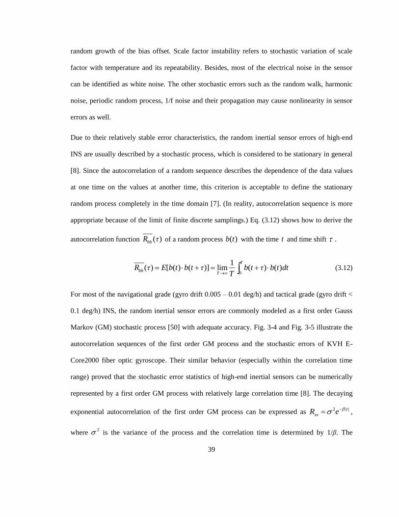
39

random growth of the bias offset. Scale factor instability refers to stochastic variation of scale

factor with temperature and its repeatability. Besides, most of the electrical noise in the sensor

can be identified as white noise. The other stochastic errors such as the random walk, harmonic

noise, periodic random process, 1/f noise and their propagation may cause nonlinearity in sensor

errors as well.

Due to their relatively stable error characteristics, the random inertial sensor errors of high-end

INS are usually described by a stochastic process, which is considered to be stationary in general

[8]. Since the autocorrelation of a random sequence describes the dependence of the data values

at one time on the values at another time, this criterion is acceptable to define the stationary

random process completely in the time domain [7]. (In reality, autocorrelation sequence is more

appropriate because of the limit of finite discrete samplings.) Eq. (3.12) shows how to derive the

autocorrelation function ( )bbR η of a random process ( )b t with the time t and time shift .

0

1( ) [ ( ) ( )] lim ( ) ( )

T

bbT

R η E b t b t η b t η b t dtT

(3.12)

For most of the navigational grade (gyro drift 0.005 – 0.01 deg/h) and tactical grade (gyro drift <

0.1 deg/h) INS, the random inertial sensor errors are commonly modeled as a first order Gauss

Markov (GM) stochastic process [50] with adequate accuracy. Fig. 3-4 and Fig. 3-5 illustrate the

autocorrelation sequences of the first order GM process and the stochastic errors of KVH E-

Core2000 fiber optic gyroscope. Their similar behavior (especially within the correlation time

range) proved that the stochastic error statistics of high-end inertial sensors can be numerically

represented by a first order GM process with relatively large correlation time [8]. The decaying

exponential autocorrelation of the first order GM process can be expressed as 2 | |

xxR e ,

where 2 is the variance of the process and the correlation time is determined by 1/β. The

40

process can be generated by passing white Gaussian noise ( )w t through a GM shaping filter,

which alters correlation characteristics of the white noise input [48] to fit the actual sensor errors.

Fig. 3-6 depicts the close loop structure of GM model shaping filter. Given a random variable b,

this filter can also be presented as a linear differential equation [50][51]:

2( ) ( ) 2 ( )b t β b t β ζ w t (3.13)

2 | |( ) β η

xx η ζR e

ηη

2ζ

21ζ

e

1corrη

β

1corrη

β

Fig. 3-4: Autocorrelation sequence of the first order Gauss Markov model

As an example, the same white noise was used to drive GM shaping filters with different

correlation parameters . Corresponding autocorrelation sequences were plotted in Fig. 3-7 to

demonstrate the influence of on statistical behavior of the first order GM process.

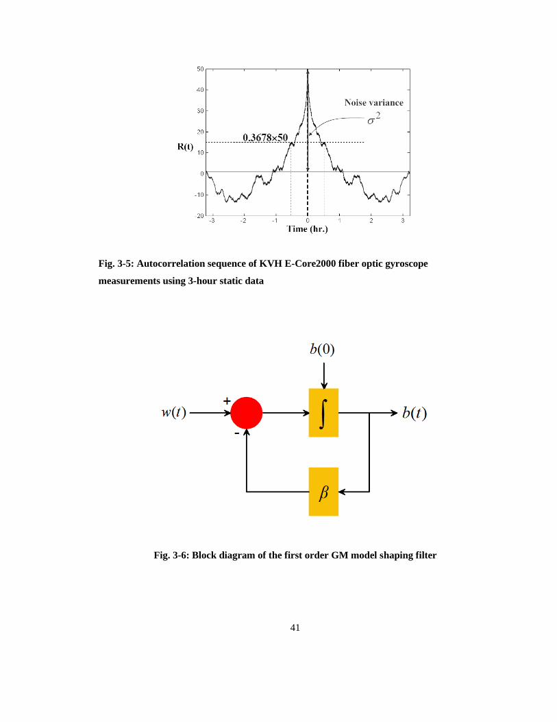
41

Fig. 3-5: Autocorrelation sequence of KVH E-Core2000 fiber optic gyroscope

measurements using 3-hour static data

Fig. 3-6: Block diagram of the first order GM model shaping filter

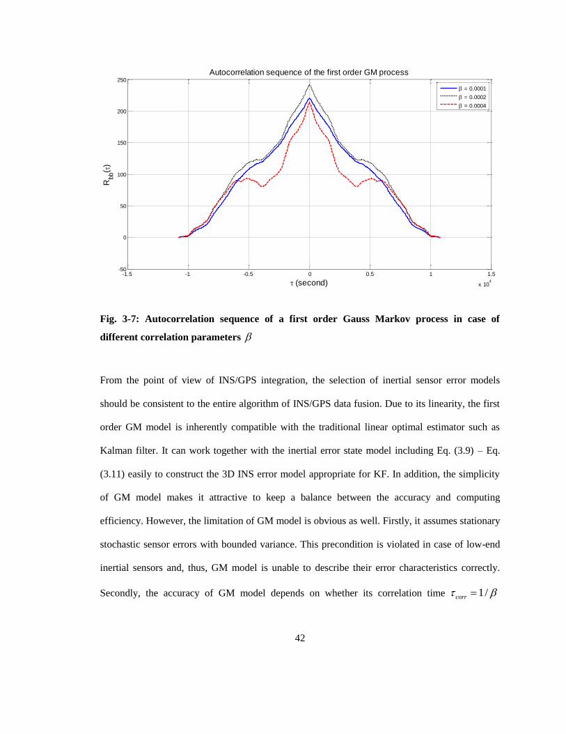
42

-1.5 -1 -0.5 0 0.5 1 1.5

x 104

-50

0

50

100

150

200

250

Autocorrelation sequence of the first order GM process

(second)

Rbb(

)

= 0.0001

= 0.0002

= 0.0004

Fig. 3-7: Autocorrelation sequence of a first order Gauss Markov process in case of

different correlation parameters

From the point of view of INS/GPS integration, the selection of inertial sensor error models

should be consistent to the entire algorithm of INS/GPS data fusion. Due to its linearity, the first

order GM model is inherently compatible with the traditional linear optimal estimator such as

Kalman filter. It can work together with the inertial error state model including Eq. (3.9) – Eq.

(3.11) easily to construct the 3D INS error model appropriate for KF. In addition, the simplicity

of GM model makes it attractive to keep a balance between the accuracy and computing

efficiency. However, the limitation of GM model is obvious as well. Firstly, it assumes stationary

stochastic sensor errors with bounded variance. This precondition is violated in case of low-end

inertial sensors and, thus, GM model is unable to describe their error characteristics correctly.

Secondly, the accuracy of GM model depends on whether its correlation time 1/corr

43

matches that of the device. In other words, because of the device differences, a static test is

inevitable and takes hours to derive corr for every inertial sensor.

3.1.4 Nonlinearity of INS Errors

Chapter 2 and subsection 3.1.3 state that bias drift, scale factor instability, and the other random

sensor errors occurred in the measuring structure and specific physical mechanism jeopardize the

performance of inertial sensors. The first order GM model or the more sophisticated higher order

autoregressive (AR) process can be utilized to describe and compensate the above errors effects

in case of high-end INS products. That is why the nonlinear INS residual errors can be safely

discarded in this scenario. However, the same assumption is not true in case of low cost MEMS-

based inertial sensors. Their more complicated error characteristics undermine the effectiveness

of either linear GM model or even higher order AR process. As a result, the nonlinear INS

residual errors discarded during the linearization process propagate and grow through the INS

mechanization procedure to generate large velocity, attitude, and position errors. They eventually

become seriously of great influence on the overall positioning accuracy.

One major drawback of MEMS gyro is zero-point stability. This is due to the difficulty in

measuring the small displacement generated by Coriolis force [17]. It may reach hundreds of

degree-per-minute or even degree-per-second. This makes sensitive algorithms such as Kalman

filter unable to correct massive background error and, thus, deteriorate the performance of

MEMS-based application in practical INS/GPS integration. In addition, for most of MEMS

devices, the instability of bias drift and scale factor could be non-stationary (evolutionary)

process that is characterized by a 1/f power spectral density [49]. This means that the best-fit

modeling of sensor errors may vary each time the system was turned on [9] or even in the same

road test. Consequently, the unstable nonlinearity dominates the outputs of low cost inertial

44

sensors such that it cannot be adequately modeled by static GM or AR models, which depend on

the stationary process.

Not only sensor errors, but also the error propagation during INS mechanization could contribute

the nonlinearity of low cost INS errors. For instance, by applying the second order Taylor series

approximation on INS mechanization equation Eq. (3.4), one can obtain Eq. (3.14), where the

over-lined parameters represent their corresponding ideal values.

.2 2

2 2 2

2

1 1

2 2

1 1 12

2 2 2

1

2

l l ll b b b b b b

l l l l l l

ie ie ie el el el l l l

l l l

V R δR δ R a δa δ a

δ δ δ δ V δV δ V

g δg δ g

(3.14)

The second order velocity error model can then be derived from Eq. (3.14) as follows:

.2 2 2

2 2

2 2 2 2

1 1 1

2 2 2

12

2

1 1 1 12

2 2 2 2

l l l

l b b b b b b b b

l l l l

ie ie el el l

l l l l l l

ie ie ie el el el l l l l

δV R δa δ a δR δ R a δa δ a

δ δ δ δ V

δ δ δ δ δV δ V δg δ g

(3.15)

For higher grade INS, since the higher order terms and cross-products in Eq. (3.15) are bounded

and small, they can be discarded, thus leaving the linear approximation of Eq. (3.15) as follows:

.

2 2l l l l l l

l b b b b ie el l ie el lδV δR a R δa δV δ δ V δg (3.16)

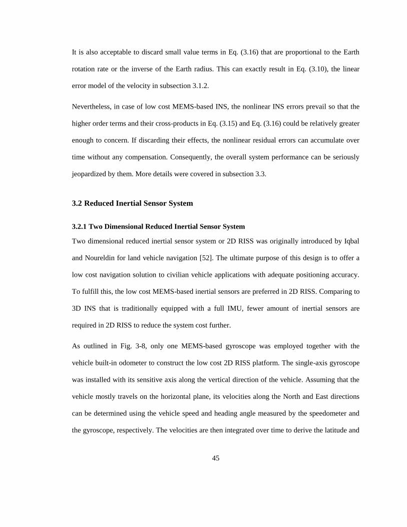
45

It is also acceptable to discard small value terms in Eq. (3.16) that are proportional to the Earth

rotation rate or the inverse of the Earth radius. This can exactly result in Eq. (3.10), the linear

error model of the velocity in subsection 3.1.2.

Nevertheless, in case of low cost MEMS-based INS, the nonlinear INS errors prevail so that the

higher order terms and their cross-products in Eq. (3.15) and Eq. (3.16) could be relatively greater

enough to concern. If discarding their effects, the nonlinear residual errors can accumulate over

time without any compensation. Consequently, the overall system performance can be seriously

jeopardized by them. More details were covered in subsection 3.3.

3.2 Reduced Inertial Sensor System

3.2.1 Two Dimensional Reduced Inertial Sensor System

Two dimensional reduced inertial sensor system or 2D RISS was originally introduced by Iqbal

and Noureldin for land vehicle navigation [52]. The ultimate purpose of this design is to offer a

low cost navigation solution to civilian vehicle applications with adequate positioning accuracy.

To fulfill this, the low cost MEMS-based inertial sensors are preferred in 2D RISS. Comparing to

3D INS that is traditionally equipped with a full IMU, fewer amount of inertial sensors are

required in 2D RISS to reduce the system cost further.

As outlined in Fig. 3-8, only one MEMS-based gyroscope was employed together with the

vehicle built-in odometer to construct the low cost 2D RISS platform. The single-axis gyroscope

was installed with its sensitive axis along the vertical direction of the vehicle. Assuming that the

vehicle mostly travels on the horizontal plane, its velocities along the North and East directions

can be determined using the vehicle speed and heading angle measured by the speedometer and

the gyroscope, respectively. The velocities are then integrated over time to derive the latitude and

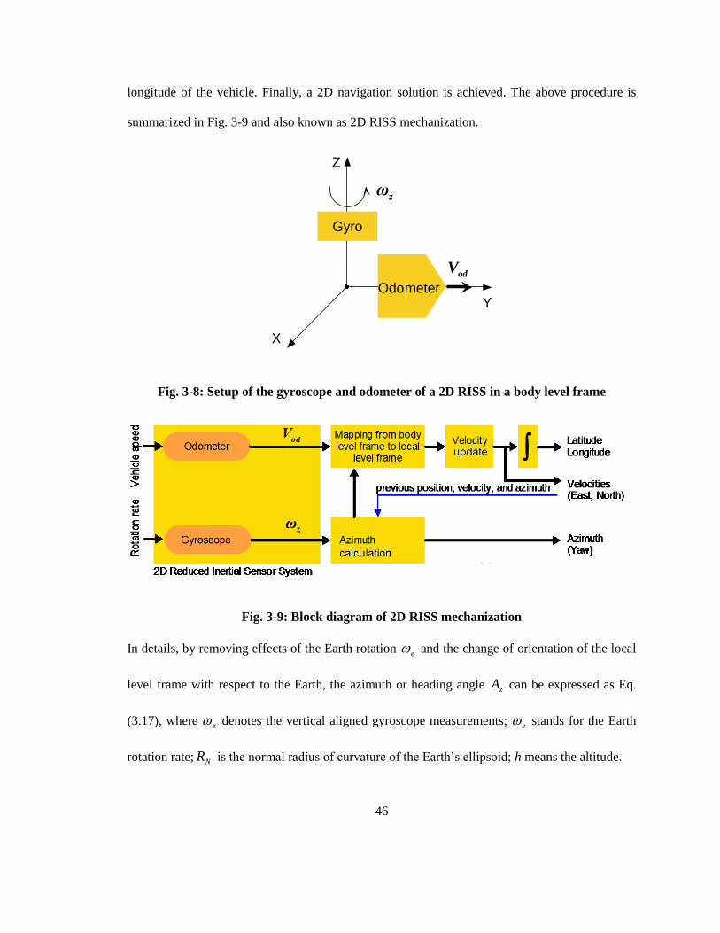
46

longitude of the vehicle. Finally, a 2D navigation solution is achieved. The above procedure is

summarized in Fig. 3-9 and also known as 2D RISS mechanization.

Gyro

zω

X

Y

Z

OdometerodV

Fig. 3-8: Setup of the gyroscope and odometer of a 2D RISS in a body level frame

Fig. 3-9: Block diagram of 2D RISS mechanization

In details, by removing effects of the Earth rotation e and the change of orientation of the local

level frame with respect to the Earth, the azimuth or heading angle zA can be expressed as Eq.

(3.17), where z denotes the vertical aligned gyroscope measurements; e stands for the Earth

rotation rate; NR is the normal radius of curvature of the Earth’s ellipsoid; h means the altitude.

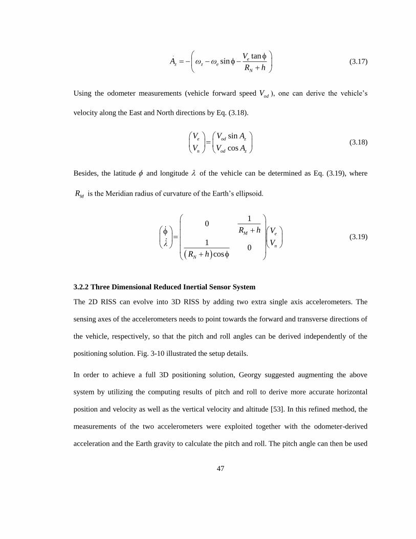
47

. tan

sin ez z e

N

VA ω ω

R h

(3.17)

Using the odometer measurements (vehicle forward speed odV ), one can derive the vehicle’s

velocity along the East and North directions by Eq. (3.18).

sin

cos

e od z

n od z

V V

V

A

AV

(3.18)

Besides, the latitude and longitude of the vehicle can be determined as Eq. (3.19), where

MR is the Meridian radius of curvature of the Earth’s ellipsoid.

1

1

cos

0

0

M e

n

N

R h

λ

h

V

V

R

(3.19)

3.2.2 Three Dimensional Reduced Inertial Sensor System

The 2D RISS can evolve into 3D RISS by adding two extra single axis accelerometers. The

sensing axes of the accelerometers needs to point towards the forward and transverse directions of

the vehicle, respectively, so that the pitch and roll angles can be derived independently of the

positioning solution. Fig. 3-10 illustrated the setup details.

In order to achieve a full 3D positioning solution, Georgy suggested augmenting the above

system by utilizing the computing results of pitch and roll to derive more accurate horizontal

position and velocity as well as the vertical velocity and altitude [53]. In this refined method, the

measurements of the two accelerometers were exploited together with the odometer-derived

acceleration and the Earth gravity to calculate the pitch and roll. The pitch angle can then be used

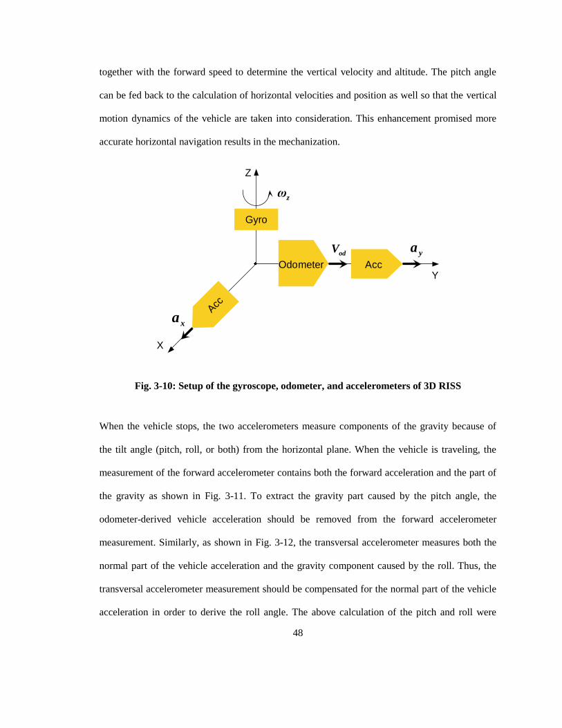
48

together with the forward speed to determine the vertical velocity and altitude. The pitch angle

can be fed back to the calculation of horizontal velocities and position as well so that the vertical

motion dynamics of the vehicle are taken into consideration. This enhancement promised more

accurate horizontal navigation results in the mechanization.

Gyro

zω

X

Y

Z

Odometer

odV

Acc

Acc

ya

xa

Fig. 3-10: Setup of the gyroscope, odometer, and accelerometers of 3D RISS

When the vehicle stops, the two accelerometers measure components of the gravity because of

the tilt angle (pitch, roll, or both) from the horizontal plane. When the vehicle is traveling, the

measurement of the forward accelerometer contains both the forward acceleration and the part of

the gravity as shown in Fig. 3-11. To extract the gravity part caused by the pitch angle, the

odometer-derived vehicle acceleration should be removed from the forward accelerometer

measurement. Similarly, as shown in Fig. 3-12, the transversal accelerometer measures both the

normal part of the vehicle acceleration and the gravity component caused by the roll. Thus, the

transversal accelerometer measurement should be compensated for the normal part of the vehicle

acceleration in order to derive the roll angle. The above calculation of the pitch and roll were

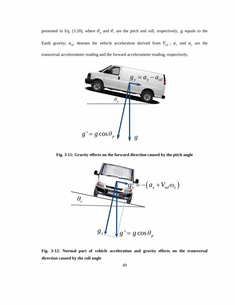
49

presented in Eq. (3.20), where p and r are the pitch and roll, respectively; g equals to the

Earth gravity; oda denotes the vehicle acceleration derived from odV ; xa and ya are the

transversal accelerometer reading and the forward accelerometer reading, respectively.

pθ

g

y y odag a

c' os pg g θ

Fig. 3-11: Gravity effects on the forward direction caused by the pitch angle

rθ

c' os pg g θ

x x od zg ωa V

zg

Fig. 3-12: Normal part of vehicle acceleration and gravity effects on the transversal

direction caused by the roll angle

50

arcsin , arcsincos

y od x od zp r

p

a a a V ωθ θ

g g θ

(3.20)

Should the pitch and roll be ready, one can derive the vertical velocity uV and altitude h

afterwards using Eq. (3.21).

sinod pu

u

θ

h

VV

V

(3.21)

Simultaneously, the pitch angle can be fed back to Eq. (3.18) with the purpose of refining the

calculation of vehicle velocities. Then, the more accurate velocities will result in more accurate

position. This eventually leads to the updated mechanization equations for 3D RISS as shown in

Eq. (3.22). Fig. 3-13 illustrated the details of this procedure.

.

1

1

cos

cos si

0 0 0 0 0 0 0 0

0 0 0 0 0 0 0 0

0 0 0 0 1 0 0 0 0

0 0 0 0 0 0 0n

cos cos

t

0

0 0 0 0 0 0 0 0

0 0 0 0 0 sin 0 0 0

0 0 0 0 0 1 0 0

0 0 0 0 0 0 0 0 0

0 0 0 0 0 0 0

a

0 0

n

M

N

e

p zn

p zu

p

z

pN

r

R

V

V

R h

λh

h

θ A

θ A

θA

θ

θ

V

R h

1

1

sin

sin

0

0

0

0

0

0

sincos

e

n

u

od e

z y od

x

y x od z

p

V

λ

ω

ω a a

g

a V

V

V

ω

g θ

V

a

a

(3.22)

51

Accelerometers

Odometer

Gyroscope

Pitch and rollcalculation

Transformation ofnavigation frames

Azimuth calculation

Position:

Velocities:

Attitude:

Acceleration

Vehicle speed

Rotation rate

x ya a

odV

zω

hλ

e n uV V V

z p rA θ θ

3D Reduced Inertial Sensor System 3D navigation resultsprevious 3D navigation results

Fig. 3-13: Block diagram of 3D RISS mechanization

3.2.3 Error Modeling of Reduced Inertial Sensor System

3D RISS error vector X consists of position error δ δλ δh , velocity error

e n uδV δV δV , azimuth error zA , and sensor measurement errors od zδa δω . Its 2D

version equals to T

e n z od zδ δλ δV δV δA δa δω instead. Apparently, these errors

are variable in time and, thus, can be described by differential equations like the 3D full INS. By

applying Taylor series approximation on Eq. (3.22) and taking the time derivative of the velocity

parts, one can establish the error model of 3D RISS as Eq. (3.23) – (3.25) :

.

z z zδ A δω A (3.23)

. .

. .

. .

sin cos cos cos

cos cos sin cos

0

0

0sin cos

e ez p od z p od

n z p od z p z n

p od p pu u

δV VA θ A θ δa

δV A θ A θ δA V

θ θ δθδ V

aV

a

a

(3.24)

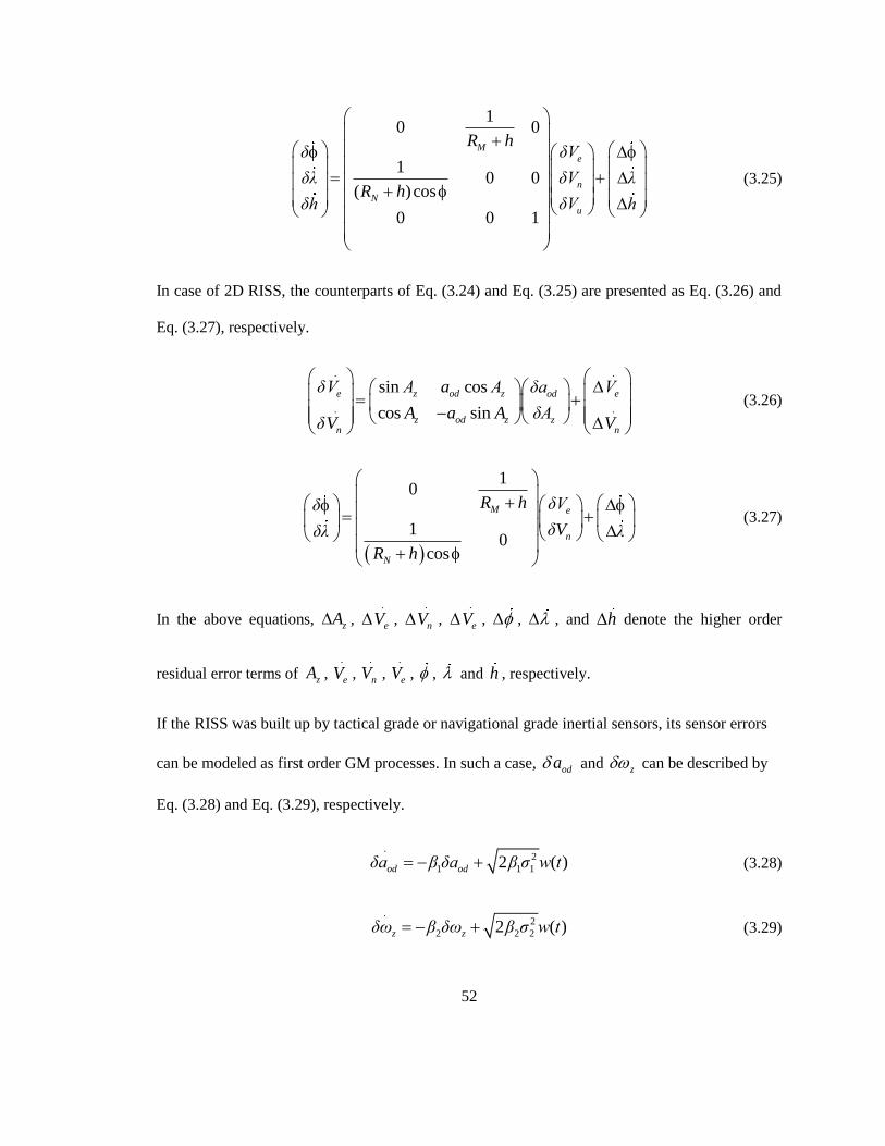
52

0 0

0 0

0 0 1

1

1

( )cos

Me

n

N

u

R hδ δV

δλ δV λR h

δh δV h

(3.25)

In case of 2D RISS, the counterparts of Eq. (3.24) and Eq. (3.25) are presented as Eq. (3.26) and

Eq. (3.27), respectively.

. .

. .

sin cos

cos sin

e z od z eod

z od z zn n

δV A A Vδa

A A δAδ

a

Va

V

(3.26)

1

1

cos

0

0

M e

n

N

R h δVδ

δδλ

hR

V λ

(3.27)

In the above equations, zA , .

eV , .

nV , .

eV , , , and h denote the higher order

residual error terms of zA , .

eV , .

nV , .

eV , , and h , respectively.

If the RISS was built up by tactical grade or navigational grade inertial sensors, its sensor errors

can be modeled as first order GM processes. In such a case, oda and z can be described by

Eq. (3.28) and Eq. (3.29), respectively.

.

2

1 1 12 ( )od odδa β δa β ζ w t (3.28)

.

2

2 2 22 ( )z zδω β δω β ζ w t (3.29)

53

For cost-sensitive applications, the high-end inertial sensors will be replaced by low-end MEMS

grade devices. In MEMS grade 3D RISS, according to Eq. (3.17) and Eq. (3.20), only the azimuth,

pitch, and roll depend on the measurements of MEMS grade inertial sensors directly. Computing

the pitch and roll from readings of the accelerometers does not include any integral operations.

Therefore, the results of these angles do not suffer from the error growth over time due to the

integration. On the other hand, the azimuth result suffers heavily from the stochastic sensor errors

of the MEMS grade gyroscope and the nonlinear inertial system errors [10]. Although the linear

azimuth error parts can be removed by linear optimal estimators, the nonlinear residual error zA

still exists and increases during the integration without any boundary. Assuming the MEMS

grade gyroscope is well aligned in an ideal case and the vehicle travels in a horizontal plane, an

uncompensated gyroscope bias wzb featured by unstable statistics and nonlinearity introduces the

remaining azimuth error z wz wzA b dt b dt , which is proportion to time t and causes an

incorrect transformation of the forward speed odV . This, in turn, introduces positioning errors in

the horizontal plane. Specifically, Eq. (3.30) and Eq. (3.31) calculate the velocity errors along the

East and North directions ( eV and nV ), which introduce higher order positioning errors (

and ) shown in Eq. (3.32). Clearly, zA accumulation will eventually deteriorate the overall

RISS performance seriously. This explains why the azimuth error is more important and requires

the nonlinear analysis.

sin sin

sin cosod z od z

e od z od z od wz z

od z

V A V AδV δV A δV A b t A

V AV

(3.30)

cos cos

cos sinod z od z

n od z od z od wz z

od z

V A V AδV δV A δV A b t A

V AV

(3.31)

54

2

2

cos sin

)

2 sin cos

cos 2 co

2(

s

2n od z od wz z

M M

e od z od wz z

N N

δV δV t A V b t Aδ dt

R h h

δV δV t A V b t Aδλ dt

h R h

R

R

(3.32)

When considering the real vehicle navigation, due to the possible misalignment and system error

propagation, zA may contain the power or cross products of the elements in linear RISS error

vector X as well. Therefore, the discrete version of Eq. (3.23) can be expressed as Eq. (3.33),

where ( )mP n are arbitrary powers or cross products of current or previous linear RISS error

elements (including the linear part of rotation rate error z ); ( )e n represents the residual error.

0

( ) ( 1)( ) ( ) ( )

Mz z

z z m m

m

δA n δA nδω n A a P n e n

t

(3.33)

Should all the ( )mP n and their weight coefficients ma be identified, the nonlinearity of the

azimuth error model can be uniquely determined.

3.3 Kalman Filter Based INS/GPS Integration

3.3.1 Kalman Filter and INS/GPS Data Fusion

Kalman filter (KF) was introduced in 1960s [54] and its first practical implementation was for

integrating inertial navigators with airborne radar aboard military aircrafts [55]. Till now, KF is

still one of the most popular algorithms allowing multi-sensor data fusion.

Kalman filter combines knowledge of the statistical nature of system errors with knowledge of

system dynamics, as represented by a state space model, to arrive at an estimate of the state of a

system [25]. In INS/GPS integration, the input of KF-based data fusion consists of external aiding

signal and INS measurements (or, mechanization results) corrupted by sensor errors and system

55

errors. Taking the difference between the aiding signals and sensing measurements as the

reference, Kalman filtering is able to optimally estimate the linear error state of the position,

velocity, and attitude. Fig. 3-14 outlines the structure of KF-based INS/GPS integration.

INSMechanization

Kalman Filter

Sensor data

GPS aiding data

_

+

+

_

INS data (L-frame)

Error prediction

Enhanced output

INS/GPS Data Fusion

Errorupdates

Fig. 3-14: Block diagram of KF-based INS/GPS integration

As a sequential recursive scheme for the optimal estimation in the sense of least mean square

errors, Kalman filter is ideal for the signal enhancement of linear discrete system driven by white

Gaussian noise. Also, it can provide real-time statistics (i.e. Kalman gain) that evaluate the

estimation accuracy. Given the sensor errors were modeled by linear GM process, Table 3-1

defines KF parameters used by INS/GPS integration. Specifically, in case of 2D RISS, the

navigation error vector in discrete domain is presented as

T

k e n z od z kδ δλ δV δV δA δa δωX at the time kt . Its discrete linear error model

can then be described by Eq. (3.34). According to Table 3-1 and Eq. (3.34), one can obtain the

sensor noise coupling matrix (or GM shaping filter parameter vector) as

2 22 20 0 0 0 0T

od od z zβ δ β δG . In parallel, the matrix 1k kF is defined in Eq.

56

(3.35) to describe the error state transition from time kt to 1kt . To execute the optimal

estimation of the error vector kX , observations of the above discrete model is required to comply

with Eq. (3.36), where kZ represents the observation vector at time kt giving the difference

between the RISS and GPS position and velocities; KH is the design matrix that links the

observation vector and the state vector in the ideal noise-free condition; kv is the vector of

observation random noise (or the stochastic error of GPS readings here), which is commonly

assumed as white sequence and independent with the RISS errors.

Table 3-1: Definition of KF parameters in INS/GPS integration

KF Parameters Definition

kX INS error state vector including errors of position, velocity, attitude and sensor

measurements

1k kF 1k k state transition matrix that updates kX and kR

kw System noise that can be viewed as white Gaussian sequence with unit variance

kG GM shaping filter parameter vector, also named as sensor noise coupling matrix

kZ Observation vector of external aiding (GPS) measurements

kv Aiding (GPS) measurement error such that 0,k Kδv N R , ·[ ] 0k kδv wE

kH Design matrix that ensures ·k k k kZ H X v

kQ Covariance matrix of system noise, [ ]T

k k kwQ E w

kR Covariance matrix of external aiding (GPS) measurement noise, [ ]T

k k kE δv δvR

kP Covariance matrix of the estimates of kX , ˆ ˆ

T

k k k k kP X X X XE

57

7 7

0 0 0 0 0 0

0 0 0 0 0 0

0 0

1

1

cos

cos sin0 0 0

0 0 0 0 0

0 0 0

sin cos

0 0 0 1

0 0 0 0 0 0

0 0 0 0 0 0

M

Ne

od z zk n

od z zz

od

odz k

z

R hδ δ

δλ

hδV

A A

R

aX I tδV

A AδA

δ

a

a

βδω

β

2

21

0

0

0

0

2

2

0

e

kn

z

od odod

z k z z

δλ

δV

δV

δA

β ζδa

δω β ζ

w

(3.34)

1

0 0 0 0 0 0

0 0 0 0 0 0

0 0 0 0 0

0 0 0 0 0

0 0 0 0 0 0 1

0 0 0 0 0 0

0 0

1

1

cos

cos sin

si

0 0 0

n

0

cos

M

N

od z zk k

od z z

od

z

R h

h

A A

A

R

A

β

β

aF

a

(3.35)

1 0 0 0 0 0 0

0 1 0 0 0 0 0

0 0 1 0 0 0 0

0 0 0 1 0 0 0

·

RISS GPS

eRISS GPS

k k k k knRISS GPS

e e

zRISS GPS

n n kod

z k

δ

δλ

δVλ λ

H X δv δvδVV V

δAV V

δa

δ

Z

ω

(3.36)

Kalman filtering, in general, has two major stages: prediction and update. Their basic mechanism

is demonstrated in Fig. 3-15 and discussed in the following.

In the prediction stage, supposing that 1ˆ ( )kX represents a posteriori estimation of previous

error state 1kX at epoch 1kt , whereas ˆ ( )kX denotes a priori estimation of current error state

kX . 1k kF , the state transition matrix, can bridge these two adjacent states using Eq. (3.37).

Simultaneously, corresponding a priori estimation of error covariance ˆ ( )kP can be determined

by a posteriori estimation 1ˆ ( )kP using Eq. (3.38).

58

Fig. 3-15: Two major stages in KF: prediction and update

In the update stage, fed by the results of the prediction stage such as ˆ ( )kX and ˆ ( )kP , the

algorithm computes a posteriori estimation of current state and error covariance according to

these a priori information and external aiding information kZ . It is worth mentioning that, in this

stage, the Kalman gain kK defined in Eq. (3.39) plays a fundamental role of not only evaluating

how well a priori estimation is, but also synthesizing reliable external reference to adjust the

accuracy of a posteriori estimation. It works as adaptive weight coefficients to manipulate the

generation of ˆ ( )kX by combining ˆ ( )kX and kZ in Eq. (3.40). Meanwhile, the decreasing

values of a priori covariance matrix elements describe how accurate the prediction is and can be

detected by kK . In Eq. (3.41), similar case occurs when determining current a posteriori

estimation of error covariance matrix ˆ ( )kP . Consequently, Eq. (3.37) – (3.41) formed the well-

known KF equation set.

1 1( )ˆ ˆ( )k k k kX F X (3.37)

59

1 1 1 1 1 1ˆ ˆ( ) ( ) T T

k k k k k k k k kF FP P QG G (3.38)

1

ˆ ( ) ( )ˆT T

K k k k k k kK PP H H H R

(3.39)

ˆ( ) ( ) ( )ˆ ˆk k k k k kX Z XX K H

(3.40)

ˆ ˆ( ) ( )k k k kH PP I K (3.41)

The procedure of prediction and update can be a recursive sequence in turns so that the linear

optimal estimation of system errors and signal enhancement of INS/GPS integration can be

achieved numerically in real-time. Fig. 3-16 shows the recursive scheme of Kalman filtering.

A prioriinformation

Initial conditions1

k k

k k k k

R

H G F

Q

0 0

ˆ ˆX P

1 1ˆ ( ) ·̂ ( )k k k kX F X

1 1 1 1 1 1

ˆ( ) · ( )· · ·ˆ T T

k k k k k k k k kF P FP G Q G

1ˆ ˆ( )· · · ( )·T T

K k k k k k kP H H P H RK

ˆ ˆ( ) ( ) · · (ˆ )k k k k k kX K H XX Z

( ) · · ( )k k k kP I HK P

kZ

Prediction stage

Update stage

Prediction oferror states

Prediction oferror

covariance

Calculate the Kalman gain

Update theestimate oferror states

Update theerror

covariance

Fig. 3-16: Recursive scheme of Kalman filtering

60

3.3.2 Limitation of KF-based INS/GPS Integration

So far, KF is still considered as one of the most popular benchmarks for INS/GPS integration

[56][57][58]. It offers navigation error predictions with adequate accuracy in case of high-end

INS. However, it has limited success if being applied on low cost MEMS-based INS/GPS

integration. In fact, the utilization of MEMS grade inertial sensors is challenged since they exhibit

more complicated error characteristics. These error effects undermined the cornerstone of KF

effectiveness, thus making the traditional method unable to guarantee the overall navigation

performance.

In brief, KF inadequacies for low cost inertial sensors can be detailed as follows:

(1) KF requires stationary stochastic modeling of sensor errors, which may not be applicable

in the environment of low cost MEMS devices. Its correct estimation of error states relies

on the accurate linear system model driven by white Gaussian noise. Nevertheless, as

mentioned before, due to the inherent non-stationary random errors, it is usually difficult

to establish a stable stochastic model for every low cost inertial sensor. Actually, the error

behavior of MEMS sensors varies in different tests and may even change in the same

running of a long term test. This reality prevents building a fixed model structure to

reflect low cost sensor errors in all scenarios.

(2) KF requires a priori information of the system and measurement covariance matrix for

each new sensor. However, it takes time to tune the corresponding parameters. Also, the

instability of MEMS sensors makes the tuning parameters that best-fit a priori

information in one time may not keep their effectiveness in another time.

(3) In KF, the weak observation of some error states may lead to unstable estimates of other

error states [59]. For instance, the weakly observable errors can be optimally estimated

61

by KF in long-term only. This makes the convergence of their error covariance very slow,

hence disturbing the stability of KF prediction of other correlated errors [60].

(4) As a time domain recursive filter, KF highly depends on short-term statistic

characteristics of data. A set of KF parameters that resulted in good estimation of error

states for one data set may not result in good estimation of error states for another data set

[61]. In other words, KF is so sensitive to local statistics that it may results in ill

prediction if there is any short term mis-modeling.

(5) As a linear optimal estimator, KF cannot suppress the nonlinear INS errors at all. Thus,

the performance of KF-only approach degrades very shortly during GPS outages.

In order to overcome limitations of the common KF, more sophisticated KF variants were

proposed as alternatives. Extened KF (EKF) uses linearized models by applying a first order

approximation on nonlinear systems [62]. However, the linearization may cause poor

performance and divergence of the filter for systems with high nonlinearity [10][63]. Unscented

KF (UKF) performs relatively better. Nevertheless, this method takes more computing time than

EKF to calculate the statistics of random variables that undergoes the nonlinear transformation

[64]. In addition, UKF is still only suitable for measurements with Gaussian distribution, which is

not applicable for MEMS sensors.

3.3.3 Current State of the Art Methods

The limitations of KF and its variants have motivated researchers to investigate alternative

methods of INS/GPS integration. The guideline is to figure out appropriate nonlinear techniques

that do not depend on linear dynamic models. The selected methods should be able to tolerate

non-stationary stochastic errors as well.

62

Recently, multilayer perception (MLP) neural networks (NN) were suggested to handle INS

errors in case of different grades of devices [34]. Research works show that a position and

velocity update architecture (PVUA) within two MLP networks could process the azimuth,

velocity, as well as position along the East and North [65]. Although MLP parameters can be

adapted by GPS aiding information, the PVUA system still has shortcomings as it cannot update

the vehicle altitude. Moreover, instead of working on INS error directly, PVUA evolves itself

based on INS position. This mechanism leads to difficulties to observe how well the system

accuracy delivers during the online navigation missions. Furthermore, due to the fact that there is

no sensitivity analysis about changing of MLP internal structure (including number of hidden

layers and neurons in each layer) currently available, the real-time implementation of this

approach has not been validated yet.

In order to develop model-free modules that mimic KF but without the needs for dynamic or

stochastic models of INS, the P P (position – position errors) structure was proposed [65]

and displayed in Fig. 3-17. Using this method, one MLP network is allocated for each position

component such that it receives INS position P as inputs and provides estimations of INS

position errors P as outputs. Consequently, the requirement of 3D positioning can be satisfied

by updating three P P networks with the help of GPS position reference. Obviously, this

method helps to profile the navigation accuracy achieved during online missions. However, its

internal structure of every MLP network still has to evolve until the best performance was

realized. This evolving procedure takes time and threats the real-time implementation seriously.

To improve P P structure, radial basis function (RBF) neural network was suggested to

replace MLP NN [66]. RBF networks can be utilized without identifying the number of neurons

in its hidden layer since these parameters are dynamically generated during the training procedure

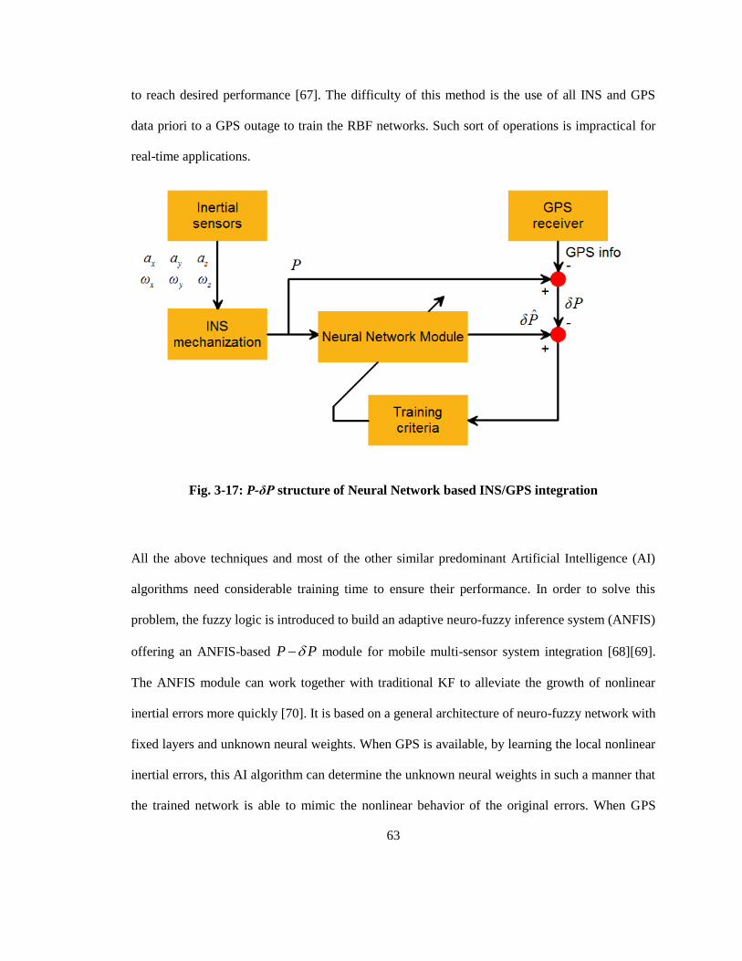
63

to reach desired performance [67]. The difficulty of this method is the use of all INS and GPS

data priori to a GPS outage to train the RBF networks. Such sort of operations is impractical for

real-time applications.

Fig. 3-17: P-δP structure of Neural Network based INS/GPS integration

All the above techniques and most of the other similar predominant Artificial Intelligence (AI)

algorithms need considerable training time to ensure their performance. In order to solve this

problem, the fuzzy logic is introduced to build an adaptive neuro-fuzzy inference system (ANFIS)

offering an ANFIS-based P P module for mobile multi-sensor system integration [68][69].

The ANFIS module can work together with traditional KF to alleviate the growth of nonlinear

inertial errors more quickly [70]. It is based on a general architecture of neuro-fuzzy network with

fixed layers and unknown neural weights. When GPS is available, by learning the local nonlinear

inertial errors, this AI algorithm can determine the unknown neural weights in such a manner that

the trained network is able to mimic the nonlinear behavior of the original errors. When GPS

64

signal is lost, the latest trained structure predicts and compensates corresponding nonlinear error

terms. Although this approach is designed to accelerate nonlinear error handling and works faster

than most of the other AI methods, its effectiveness has been verified only in the post-processing.

There still exist challenges to apply it in real-time applications. Moreover, like the other AI

methods, the performance of ANFIS highly depends on the consistency of the training data and

show limited success if the error dynamics do not stay the same between their training and

prediction stages. The above limitations restrain the utilization of ANFIS in real-time MEMS-

based INS/GPS integration.

The inadequacies of AI-based nonlinear methods motivate their replacement by more

sophisticated nonlinear techniques. Targeting on low cost INS/GPS integration, MEMS-based

INS error reduction, and their real-time implementation, this study suggested fast orthogonal

search algorithm, a nonlinear system identification approach, as the solution. Inspired by P P

structure, the proposed method is conducted by referring the AI research progress mentioned

above. More details were discussed in the following chapters.

65

Chapter 4

Fast Orthogonal Search Algorithm

4.1 Review of Fast Orthogonal Search (FOS)

Fast Orthogonal Search (FOS) algorithm was originally introduced by Korenberg as a general

purpose numerical technique to build difference equations or functional expansions of nonlinear

systems and for time series analysis [71]. Without any a priori knowledge about the system of

interest, FOS works directly on the system inputs and outputs. It keeps on searching for the most

significant higher order terms or cross-products of system inputs and outputs recursively until

certain stopping criteria are met. Using this method, FOS modeling is able to best-fit the

nonlinear system with unknown structure in the form of a parsimonious multidimensional

polynomial of system input and output values [72]. Owing to its ability to detect important

nonlinear factors as well as their contribution to the system nonlinearity, FOS has been widely

applied in time series analysis, short-term signal processing, nonlinear system identification and

so forth [73][74].

Without loss of generality, a causal nonlinear system, such as the error model of MEMS grade

inertial sensor system, can be represented as a difference equation like Eq.(4.1):

, ( ),( ) [ ( 1), ( ), , ( )] ( )y n K x n x n L e ny n F y n (4.1)

where [ ]F is a polynomial with unknown structure, ( )x n and ( )y n are system inputs and

outputs, respectively. ( )e n denotes the residual error. Assuming the maximum delays of ( )x n

and ( )y n are finite and up to 0 0 0(1 ,0 )N K N L N , the ultimate goal of FOS algorithm is

to identify the architecture of polynomial [ ]F by collecting the most significant higher order

terms or cross-products of system inputs and outputs that contribute to the system nonlinearity.

66

4.2 Polynomial Representation of Nonlinear System

It is clear that Eq.(4.1) can be simplified as a polynomial expansion like Eq.(4.2):

0

0

( ) ( ), ( )) 1(M

m m

m

a P n ey n n P n

(4.2)

where 0( ) |m mP n are arbitrary higher order terms or cross-products relying on { ( )}iy n k and /

or { ( )}jx n l (note: 0 00:1 , 0 :0i ji k N j l N ); ma and M are the weight

coefficients and the pre-defined maximum amount of model terms ( )mP n , respectively; ( )e n

presents the residual error. In order to identify the polynomial structure, the FOS algorithm

generates a group of arbitrary candidate terms for the ( )mP n first. It can then examine the non-

orthogonal candidates for the ( )mP n in sequence and select the most appropriate ones as the

nonlinear model terms. Each time, the candidate for ( )mP n with the maximum reduction of

mean-square-error (m.s.e.) between the outputs of the FOS model and the original nonlinear

system will be selected, given the terms already chosen for the model. Meanwhile, after

excluding those candidates that have already been selected for the model terms, the resulting

subset of the previous candidate group becomes the new candidate pool to enable searching of the

next appropriate candidate. This procedure runs recursively until reaching pre-defined stopping

criteria.

To accelerate candidate searching, FOS creates a set of orthogonal bases by orthogonalising the

candidate pool using an implicit Gram-Schmidt (GS) routine. Every candidate term can then be

identified in the functional space defined by the orthogonal bases. After applying this operation,

FOS produces an economical orthogonal polynomial expansion of the system output ( )y n as

Eq.(4.3):

67

0

( () ( ) )M

m m

m

gy n W n e n

(4.3)

where the mg are the weights of the orthogonal terms ( )mW n in the sense of least-mean-square

model-fit; ( )e n denotes the residual errors. In principle, the GS routine generates GS coefficients

mr and the orthogonal term ( )mW n by taking the current non-orthogonal term ( )mP n and the

weighted combination of revealed orthogonal terms ( )rW n into consideration. Eq. (4.4) describes

the iterative process:

1

20

( ) ( ), ( ) ( ) ( )

( )

mm r

mr m m mr r

rr

P n W nn P n W n

W nW

(4.4)

where 0,1, ,m M ; 0,1, ,r m ; the over-scores here and following denote the time

average from 0n N to n N .

The power of FOS here is that it is able to bypass the explicit derivation of the ( )mW n and obtain

the mr faster. This strategy accelerates the calculation of the orthogonal weights mg as well

since the mr can be utilized in turn to determine mg as discussed later.

4.3 Implicit Gram-Schmidt Orthogonal Search of Candidates

Instead of allocating space for every orthogonal term ( )mW n , the implicit building of ( )mW n

reduces computing complexity and memory requirements significantly. The orthogonality

principle [48] states that two functions are mutually orthogonal if the time average of their

products or the expected value of their correlation is equal to zero. To compute mr in terms of

68

orthogonality principle without calculating ( )rW n , the function ( , )D m r is defined in Eq(4.5) to

present the correlation of the candidate function and the orthogonal term.

( ) ( ), 1, , ; 1,, ) ,( m rP n W n mD m Mr r m (4.5)

According to Eq.(4.4), Eq.(4.5) is identical to Eq.(4.6):

1

20

( ) ( ) ( , )( ) ( ) ( , ),(

))

, )(,

(

rr i

m r ri ri

i i

P n W n D r iP n P n D mD m r i

D i iW n

(4.6)

where ri are the GS coefficients; ( , )D i i equals 2( )iW n due to the orthogonality principle.

Indeed, given the initial conditions such as (0,0) 1D and ( ,0) ( )mD m P n , Eq.(4.6) provides

a numerical scheme to derive ( , )D m r and mr recursively without explicitly calculating

( )mW n .

When all the GS coefficients mr are ready, they can be used to determine the weights of

orthogonal terms mg directly. The idea is to figure out the value of mg that causes the maximum

reduction of the model-fit m.s.e. defined in Eq.(4.7).

2 2 2 2

0

(. . . ) ( ) ( )M

m mm

m

e n y n g Wm s e n

(4.7)

By differentiating Eq.(4.7) with respect to mg and taking Eq.(4.3) into consideration, Eq.(4.8)

derives the desired value of mg :

2

( ) ( )

( )

mm

m

y n W ng

W n (4.8)

69

To bypass the explicit calculation of the orthogonal term ( )mW n in Eq.(4.8), the function ( )C m

is defined in Eq.(4.9) to present the correlation of the original system output ( )y n and ( )mW n .

1

0

( ) ( ) ( ) ( ) ( ), (0) ( ), 1,( ,)m

m m mr

r

y n W n P n y n C r C yC m n m M

(4.9)

In return, the calculation of mg can only depend on ( , )D m r and ( )C m as shown in Eq.(4.10).

2

( ) ( ) ( ), 1, ,

( , )( )

mm

m

y n W n C mm M

D m mW ng (4.10)

Meanwhile, Eq.(4.11) proves that derivation of the model-fit m.s.e. reduction mQ offered by the

selected candidate can benefit from ( , )D m m as well.

2 2 2

1 ( ). . . . . . ( , )m m m m mmm s e m s e Q g D mg mW n (4.11)

mQ is critical for the selection of the candidate term for ( )mP n as the candidate with the

maximum value of mQ will be added to the FOS model.

Eqs. (4.6), (4.9), (4.10), and (4.11) show that the updating of ( , )D m r , mr , ( )C m , mg , and

mQ can be achieved during the iterations with no need of deriving orthogonal terms ( )mW n . This

recursive procedure continues until either of the following stopping criteria has been met:

Model-fit m.s.e. is smaller than a pre-defined threshold.

The number of selected candidates has reached its pre-defined upper limit.

There are no remaining candidates offering significant m.s.e. reduction. (i.e.: their mQ

values are smaller than that expected from fitting white Gaussian noise.)

70

Actually, in such a way, FOS manages to implicitly decompose the system output ( )y n in the

orthogonal function space defined by ( )mW n . To re-construct the nonlinear model from the space,

mr and mg are then related back in Eq.(4.12) to determine the model coefficients ma .

1

(, , 1, 1 , ,)M i

m i i i ir r m

i m r m

g v va v v i m M

(4.12)

As the weights of the selected candidates in Eq. (4.2), the { }ma identify the system nonlinearity

and represent the final results of FOS modeling. The kernel operations of FOS algorithm are

summarized in Fig. 4-1. More details about FOS can be found in [71] - [75].

Fig. 4-1: Block diagram of Fast Orthogonal Search algorithm

71

4.4 Merits of FOS Algorithm

Observing Eq. (3.33) and (4.2), it is clear that FOS provides a practical approach to identify

higher order RISS errors. Instead of mathematical derivation, this numerical algorithm can work

on true RISS error data directly. Thus, during GPS availability, corresponding information

enables FOS to adapt the model structure online. Simultaneously, by selecting candidate

functions according to the model-fit m.s.e. reduction, FOS can always detect the most significant

error terms as well as their weight coefficients. Hence, even using a short range of training data, it

is still able to best-fit RISS error dynamics without any a priori knowledge about the system. In

comparison to other algorithm like ANFIS, FOS does not mimic nonlinear system dynamics. It

identifies higher order error terms as a mathematical model in terms of their significance and uses

them to update the architecture of the nonlinear model online. As a result, the prediction of the

FOS model keeps stable accuracy even if the dynamic behavior of the vehicle varies between the

modeling and prediction stages. On the other hand, the ANFIS method acquires knowledge of the

nonlinear system from the local training data. Therefore, its performance highly relies on the

consistency of the training data. Changes of the local error statistics are very common for a

MEMS device but will undermine reliability of AI training and prediction. This explains why AI

approach performs well in GPS outages of shorter time ( 45 sec) [10] while FOS can offer the

same or better results in GPS outages with longer duration (e.g. 2 min). Moreover, due to its

tolerance of non-stationary stochastic sensor errors, FOS has proven itself adept at removing both

colored and white noise from the modeling errors, which cannot be handled by KF. This

introduces important advantages when processing IMU measurements corrupted by unstable

MEMS sensor errors.

Regarding the computational efficiency, FOS is attractive to rapidly build an accurate RISS error

model in real-time. It is worth mentioning that the creation of the orthogonal functions ( )mW n in

72

Eq.(4.3) is expensive in computing time and memory. FOS bypasses this problem by taking a

more efficient strategy. Instead of working directly on the ( )mW n , it conducts an implicit

orthogonal search using a Cholesky decomposition, as suggested by Korenberg [72]. In addition,

all the time average values on the right side of Eqs. (4.6), (4.9), (4.10) and (4.11) can be

calculated once and for all at the outset or as needed and stored. Hence, when testing new

candidate functions, FOS can benefit rapidly from the off-the-shelf time average values related to

the last chosen candidate. This saves computing time and memory space, which are of specific

interest for real-time nonlinear modeling and embedded vehicle applications. To verify this

characteristic, Chapter 7 demonstrates the running of the FOS algorithm on a general purpose

digital signal processor in order to enable online vehicular navigation.

All the above features ensure the advantages of the FOS algorithm on building nonlinear error

models more quickly than AI-based methods (e.g., ANFIS module). Moreover, estimation

techniques that require an accurate nonlinear model can receive support from FOS as well. For

instance, the FOS model can work together with a Particle Filter (PF – a nonlinear estimator) to

provide more accurate positioning prediction.

73

Chapter 5

Cascade of Kalman Filter and Fast Orthogonal Search for MEMS –

Based INS/GPS Integration

5.1 Augmented KF/FOS Module

In order to apply the FOS algorithm to the integration of low cost INS and GPS, this study

proposed an augmented KF/FOS module for vehicular navigation. The idea is to keep KF

modeling and predicting the linear INS error parts, while leaving the nonlinear residual errors and

possible mis-modeling aftermath of KF to be handled by FOS. The entire design is deployed and

verified on different MEMS – based RISS/GPS platforms described in the following subsections.

As mentioned in Chapter 3, higher order azimuth error is the major source of nonlinear RISS

errors. Therefore, FOS is cascaded to KF with the purpose of modeling and estimating the

nonlinear azimuth error.

5.1.1 Modeling Stage

When GPS signal is available, the KF/FOS module works in the modeling stage. Its KF part

operates as usual to predict linear RISS errors and update these estimations using GPS aiding

information. In parallel, the KF prediction outputs are sent to FOS as the training data.

Specifically, in Eq. (5.1), KF azimuth error prediction KF

zA is utilized together with RISS

mechanization result mec

zA and GPS aiding azimuth gps

zA to derive the true nonlinear azimuth

residual error zA (including rotation rate error effects) appeared also in Eq. (3.33).

mec KF gps

z z z zA A A A (5.1)

74

Fig. 5-1: Modeling stage of KF/FOS module during GPS availability

As the desire output, zA plays the role of training data to enable FOS modeling of the azimuth

residual error. Simultaneously, FOS routine creates possible candidate terms using KF prediction

outputs in the background. The procedure results in the fact that the candidate terms here consist

of higher order terms or cross products relying on the linear error estimations of position (KFP ),

velocities (KFV ), azimuth (

KF

zA ), gyroscope measurement (KF

z ), and odometer-derived

acceleration (KF

oda ). By launching an implicit orthogonal search on the candidates using the

75

scheme mentioned in Chapter 4, FOS algorithm can then construct an accurate model of the

nonlinear azimuth error. Fig. 5-1 depicts the modeling stage of KF/FOS module.

5.1.2 Prediction Stage

Once GPS outages occur, the KF/FOS module operates in the prediction stage. Due to the

absence of GPS aiding signals, KF predictions of linear RISS errors (KFP ,

KFV , and KF

zA )

do not have any chance to be updated or corrected. They are passed as the inputs to drive the

latest pre-built FOS model. Since this FOS model is supposed to best-fit the nonlinearity of

azimuth errors at the beginning of every GPS outage, it is expected to output reliable nonlinear

azimuth error predictions [ ]zE A throughout the missing duration of GPS signals. [ ]zE A can

then be used together with KF predicted linear azimuth error KF

zA and the unaided

mechanization result mec

zA to derive the corrected azimuth *

zA as Eq. (5.2).

Fig. 5-2: Prediction stage of KF/FOS module during GPS outages

76

* [ ]mec KF

z z z zA AA E A (5.2)

When the corrected azimuth *

zA is ready, a new standalone RISS mechanization labeled (B) in

Fig. 5-2 can start and benefit from *

zA to calculate more accurate position *P and velocities

*V .

Consequently, the proposed KF/FOS module is able to enhance navigation performance during

GPS outages.

5.2 Two Dimensional Vehicular Navigation using KF/FOS Module

KF/FOS module is firstly introduced to two-dimensional (2D) vehicular navigation in order to

examine its effectiveness on improving navigation performance. Several road test experiments

were carried out in a land vehicle using the equipment mentioned in subsection 5.2.1. Among

these experiments, three road test trajectories in various typical scenarios are demonstrated and

discussed in details. The results confirm that, during GPS outages, the proposed method is able to

enhance the positioning accuracy drastically by correcting nonlinear azimuth errors and the

horizontal positioning errors.

5.2.1 Experimental Setup of 2D RISS

As mentioned in Chapter 3, the 2D RISS platform used in this research consists of only one

gyroscope and the vehicle built-in odometer. The gyroscope is a MEMS-based sensor from the

Crossbow IMU300CC-100 shown in Fig. 5-3. Its sensitive axis is aligned along with the vertical

direction of the vehicle frame. Being measured by the vehicle built-in odometer, the forward

speed is logged in through an on-board diagnostic version II (OBD II) interface using a device

called CarChip [76]. The CarChip is displayed in Fig. 5-4.

77

Fig. 5-3: Crossbow IMU300CC-100 [77]

The above devices are integrated to establish a MEMS-based 2D RISS. This system can then

work together with a GPS receiver as a low cost testing platform using the suggested

methodology.

Fig. 5-4: CarChip® driving and engine performance monitor from Davis Instruments [76]

To thoroughly evaluate the results of KF/FOS module on the 2D RISS, a reliable navigation

reference is required to compare with. In this study, the reference solution is supplied by an off-

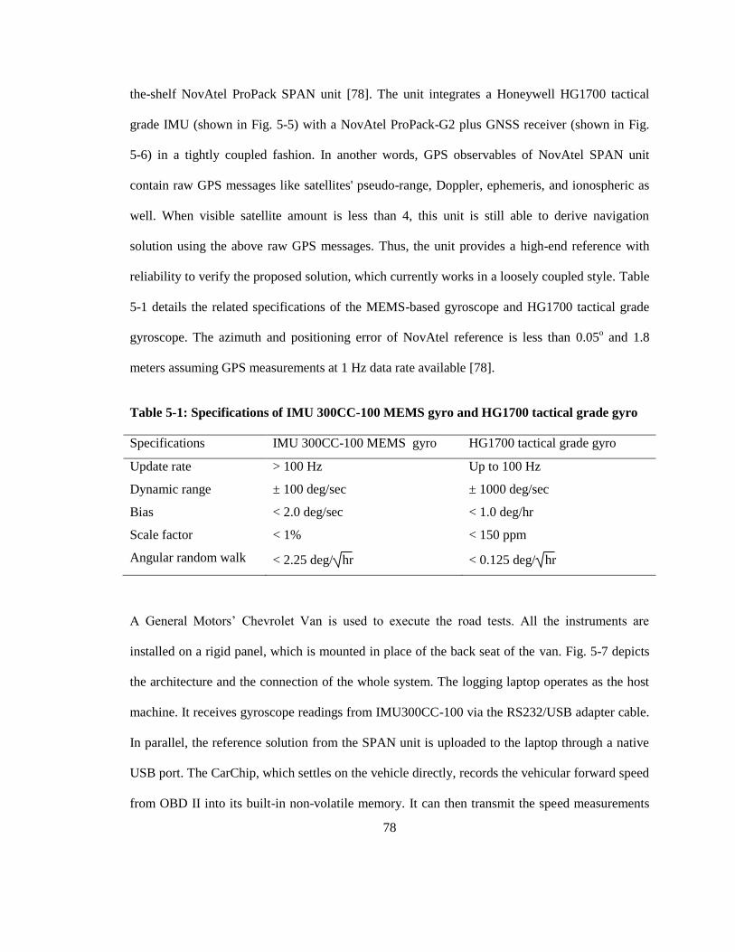
78

the-shelf NovAtel ProPack SPAN unit [78]. The unit integrates a Honeywell HG1700 tactical

grade IMU (shown in Fig. 5-5) with a NovAtel ProPack-G2 plus GNSS receiver (shown in Fig.

5-6) in a tightly coupled fashion. In another words, GPS observables of NovAtel SPAN unit

contain raw GPS messages like satellites' pseudo-range, Doppler, ephemeris, and ionospheric as

well. When visible satellite amount is less than 4, this unit is still able to derive navigation

solution using the above raw GPS messages. Thus, the unit provides a high-end reference with

reliability to verify the proposed solution, which currently works in a loosely coupled style. Table

5-1 details the related specifications of the MEMS-based gyroscope and HG1700 tactical grade

gyroscope. The azimuth and positioning error of NovAtel reference is less than 0.05o and 1.8

meters assuming GPS measurements at 1 Hz data rate available [78].

Table 5-1: Specifications of IMU 300CC-100 MEMS gyro and HG1700 tactical grade gyro

Specifications IMU 300CC-100 MEMS gyro HG1700 tactical grade gyro

Update rate > 100 Hz Up to 100 Hz

Dynamic range ± 100 deg/sec ± 1000 deg/sec

Bias < 2.0 deg/sec < 1.0 deg/hr

Scale factor < 1% < 150 ppm

Angular random walk < 2.25 deg/ hr

< 0.125 deg/ hr

A General Motors’ Chevrolet Van is used to execute the road tests. All the instruments are

installed on a rigid panel, which is mounted in place of the back seat of the van. Fig. 5-7 depicts

the architecture and the connection of the whole system. The logging laptop operates as the host

machine. It receives gyroscope readings from IMU300CC-100 via the RS232/USB adapter cable.

In parallel, the reference solution from the SPAN unit is uploaded to the laptop through a native

USB port. The CarChip, which settles on the vehicle directly, records the vehicular forward speed

from OBD II into its built-in non-volatile memory. It can then transmit the speed measurements

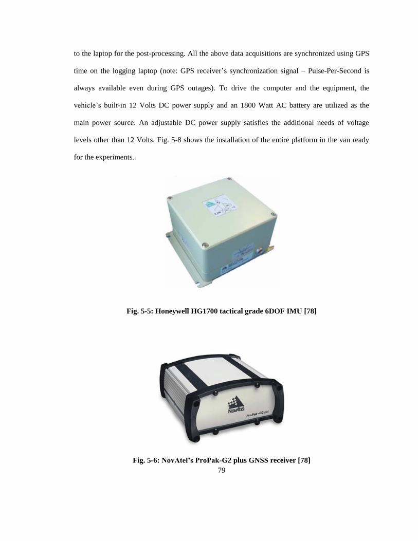
79

to the laptop for the post-processing. All the above data acquisitions are synchronized using GPS

time on the logging laptop (note: GPS receiver’s synchronization signal – Pulse-Per-Second is

always available even during GPS outages). To drive the computer and the equipment, the

vehicle’s built-in 12 Volts DC power supply and an 1800 Watt AC battery are utilized as the

main power source. An adjustable DC power supply satisfies the additional needs of voltage

levels other than 12 Volts. Fig. 5-8 shows the installation of the entire platform in the van ready

for the experiments.

Fig. 5-5: Honeywell HG1700 tactical grade 6DOF IMU [78]

Fig. 5-6: NovAtel’s ProPak-G2 plus GNSS receiver [78]

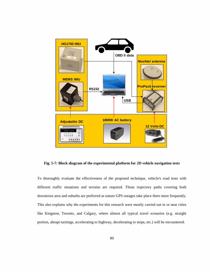
80

HG1700 IMU

MEMS IMU

12 Volts DC

1800W AC batteryAdjustable DC

NovAtel antenna

ProPack receiver

USB

RS232

OBD II data

Fig. 5-7: Block diagram of the experimental platform for 2D vehicle navigation tests

To thoroughly evaluate the effectiveness of the proposed technique, vehicle's road tests with

different traffic situations and terrains are required. Those trajectory paths covering both

downtown area and suburbs are preferred as nature GPS outages take place there more frequently.

This also explains why the experiments for this research were mostly carried out in or near cities

like Kingston, Toronto, and Calgary, where almost all typical travel scenarios (e.g. straight

portion, abrupt turnings, accelerating to highway, decelerating to stops, etc.) will be encountered.

81

Fig. 5-8: Installation of the equipment inside the van for 2D road tests

Three road test trajectories using the above setup are presented in this study. The ultimate aim is

to examine the navigation performance of KF/FOS module in GPS-denied environments. Hence,

for each trajectory, several artificial GPS outages were intentionally introduced. During these

outages, the results of the proposed method are compared to those of the KF-only approach. The

positioning errors of both approaches are derived with respect to the NovAtel reference.

To build candidate terms for FOS algorithm, either a 60-second or a 100-second sliding window

is employed to collect the true RISS error data. In every 60-second or 100-second window during

GPS availability, the construction of the azimuth error model takes 0.0185 seconds or 0.0768

seconds on average, respectively. These results came from an executable FOS-toolkit developed

by author on an Intel Pentium-4 2.80 GHz 80x86-compatible processor with 2GB DDR2 RAM.

Honeywell HG1700

High-end IMU

Crossbow IMU-300CC-100 MEMS

IMU

ProPak-G2 plus GNSS receiver

82

Using the same conditions, the modeling of azimuth errors can take several seconds for AI

algorithm such as ANFIS module. Details in Table 5-2 show that FOS has better computing

efficiency and is able to work in real-time.

Table 5-2: Real-time performance of FOS modeling of nonlinear azimuth errors in 2D tests

60-second sliding window

Maximum number of possible candidate terms > 7000

Maximum number of the selected candidate terms 30

Average time cost of FOS modeling 0.0185 seconds

Maximum time cost of FOS modeling < 0.08 seconds


Maximum number of possible candidates > 7000




5.2.2 The First Trajectory

The first road test trajectory is a round trip between Kingston and Napanee, Ontario, Canada. As

shown in Fig. 5-9, in about 100 minutes, the testing vehicle traveled over 96 km continuously on

either urban streets or highway sections. In order to evaluate the positioning accuracy of KF/FOS

module during GPS signal blockage, up to 10 artificial GPS outages were intentionally

introduced in the post-processing. They were also indicated by circles overlaid on the map in Fig.

5-9.

83

Fig. 5-9: Road test trajectory between Kingston and Napanee. Circles indicate the location

of GPS outages.

The KF/FOS module was applied on this road test trajectory twice, once for 60-second outages

and once for 120-second outages. To cover all conditions of a typical trip, the outages were

selected such that their locations involve straight portions, turns, slopes, high vehicle speeds, low

vehicle speeds, and stops. Regarding the FOS modeling during GPS availability, a 100-second

sliding window is used for this trajectory to collect the training data.

1. Results in case of 60-second GPS outages

Table 5-3 and Fig. 5-10 show the maximum errors and the root-mean-square (RMS) errors in the

2D horizontal position during all the 60-second GPS outages for both KF/FOS and KF-only

methods. By comparing their results, it is obvious to see the effectiveness of the proposed

technique. In each GPS outage (except outage #9), the KF/FOS module offered more than 60%

enhancement in positioning accuracy over KF-only solution. This is due to the fact that FOS is

able to model and suppress the nonlinear azimuth error, which cannot be handled by KF or the

linearized error models.

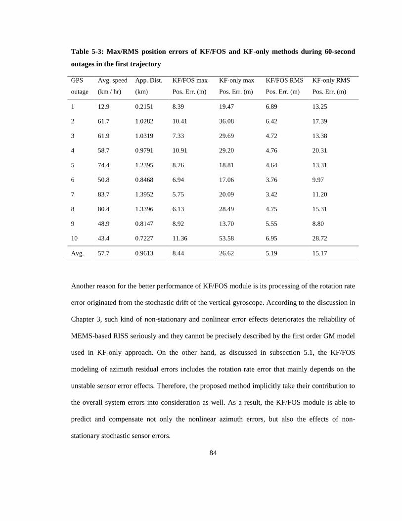
84


outages in the first trajectory

GPS

outage

Avg. speed

(km / hr)

App. Dist.

(km)

KF/FOS max

Pos. Err. (m)

KF-only max

Pos. Err. (m)

KF/FOS RMS

Pos. Err. (m)

KF-only RMS

Pos. Err. (m)

1 12.9 0.2151 8.39 19.47 6.89 13.25

2 61.7 1.0282 10.41 36.08 6.42 17.39

3 61.9 1.0319 7.33 29.69 4.72 13.38

4 58.7 0.9791 10.91 29.20 4.76 20.31

5 74.4 1.2395 8.26 18.81 4.64 13.31

6 50.8 0.8468 6.94 17.06 3.76 9.97

7 83.7 1.3952 5.75 20.09 3.42 11.20

8 80.4 1.3396 6.13 28.49 4.75 15.31

9 48.9 0.8147 8.92 13.70 5.55 8.80

10 43.4 0.7227 11.36 53.58 6.95 28.72

Avg. 57.7 0.9613 8.44 26.62 5.19 15.17

Another reason for the better performance of KF/FOS module is its processing of the rotation rate

error originated from the stochastic drift of the vertical gyroscope. According to the discussion in

Chapter 3, such kind of non-stationary and nonlinear error effects deteriorates the reliability of

MEMS-based RISS seriously and they cannot be precisely described by the first order GM model

used in KF-only approach. On the other hand, as discussed in subsection 5.1, the KF/FOS

modeling of azimuth residual errors includes the rotation rate error that mainly depends on the

unstable sensor error effects. Therefore, the proposed method implicitly take their contribution to

the overall system errors into consideration as well. As a result, the KF/FOS module is able to

predict and compensate not only the nonlinear azimuth errors, but also the effects of non-

stationary stochastic sensor errors.

85



As shown in Eqs. (3.30) – (3.32), the RISS error in position depends on the product of outage

duration, azimuth error, and vehicle velocities. When the vehicle experienced considerable

motion dynamics (heading angle change > 90o) or higher speeds (> 65 km/hr), the nonlinear RISS

errors increase rapidly over time and become the major source of the overall system error. By

attenuating their influence, the KF/FOS module outperforms the KF-only approach dramatically

during GPS outages #2, #3, #7, and #8. On average, the maximum position errors of the KF/FOS

and KF-only solutions are 8.44 meters and 26.62 meters, respectively, in about 0.96 km.

2. Significance of nonlinear azimuth error

As the only MEMS device used in this study, the vertical gyroscope suffers from its unstable

stochastic drift, which intensifies the importance of azimuth errors further. This random error of

low-cost MEMS-based gyroscope and, consequently, the azimuth errors are not adequately

modeled by KF, which relies on its linear or linearized models for the stochastic sensor error such

as Gauss Markov process. This explains why, during GPS outages, the residual and higher order

errors of the azimuth are the key points for the performance of 2D MEMS RISS. FOS algorithm

was applied to handle these residual and nonlinear error components after the KF prediction.

86

To have a better view of FOS role in modeling the residual and nonlinear errors not well

compensated by KF, Fig. 5-11 and Table 5-4 show the maximum azimuth error during all the 60-

second GPS outages of the first trajectory for both KF-only and KF/FOS methods. Apparently,

the azimuth error of KF-only solution becomes dominant in each GPS outage. It involves the

insufficiently modeled gyroscope drift and the un-modeled higher order error terms. These error

components grow over time and result in increasing incorrect shifts of the azimuth, thus causing

severe heading deviation quickly. FOS algorithm prevents the above cases by modeling and

predicting the nonlinear azimuth error and the other residual errors that were not managed by KF.

Their effects were mostly compensated by the FOS model outputs during all the GPS outages.

This makes the azimuth error of KF/FOS module decrease drastically. For instance, before

cascading FOS to KF, as outlined in Table 5-4, the average value of the maximum azimuth error

during the 10 outages is greater than 7◦ for KF-only method. KF/FOS module reduced this value

to 1.19◦ after its azimuth correction. GPS outage #4 is more challenging as the vehicle

experienced a heading angle change over 90o with abrupt decelerations in it. Although KF/FOS

enhancement on azimuth accuracy is less prominent in this outage, it still provides much better

performance than KF-only. These results demonstrate the significance of the nonlinear azimuth

error on 2D MEMS-based RISS and the effectiveness of KF/FOS module in suppressing them.

Fig. 5-11: Maximum azimuth errors during 60-second GPS outages of the first trajectory

87

Table 5-4: Maximum azimuth errors of KF-only and KF/FOS methods during 60-second

outages of the first trajectory

GPS outage 1 2 3 4 5 6 7 8 9 10 Avg.

KF-only max

azi. err. (deg)

5.67 14.99 11.95 10.30 5.44 2.64 2.51 4.16 7.50 13.40 7.86

KF/FOS max

azi. err. (deg)

1.28 0.76 0.36 4.64 0.52 1.43 0.30 1.06 0.60 0.92 1.19

3. Results in case of 120-second GPS outages

Fig. 5-12 and Table 5-5 show the maximum errors and the RMS errors in the 2D horizontal

position during all 120-second GPS outages for both KF/FOS and KF-only methods. Like the

previous results, the proposed module outperformed KF-only solution in all the 120-second

outages. On average, their maximum position errors are 20.99 meters and 59.08 meters,

respectively, in approximately 2 km. The azimuth error originates from the drift of the MEMS-

based gyroscope that cannot be well corrected by KF. Thus, it accumulates in proportion to the

outage duration and, in turn, leads to the rapid error growth in position proportional to the square

of outage duration. As a result, the accuracy enhancement, which relies on the FOS-based

reduction of both the gyroscope drift and the azimuth error, becomes more apparent in case of

120-second GPS outages. These results also prove that KF/FOS module is able to tolerate non-

stationary stochastic sensor errors in longer terms.

Fig. 5-13, Fig. 5-15, and Fig. 5-17 give the zoom-in sections of this trajectory during 120-second

GPS outage #4, #6, and #8. Both KF/FOS solution and KF-only solution are plotted together with

the reference route on these figures. To thoroughly investigate the motion dynamics as well as

their influence on the system performance, Fig. 5-14, Fig. 5-16, and Fig. 5-18 illustrate the

88

vehicle forward speed and azimuth during the above outages, respectively. The information of the

speed and heading angle are offered by the NovAtel reference.





GPS

outage

Avg. speed

(km / hr)

App. Dist.

(km)

KF/FOS max

Pos. Err. (m)

KF-only max

Pos. Err. (m)

KF/FOS RMS

Pos. Err. (m)

KF-only RMS

Pos. Err. (m)

1 35.6 1.1862 35.20 57.13 15.43 26.44

2 58.7 1.9582 19.43 65.87 12.83 38.71

3 68.9 2.2970 19.16 83.00 9.34 39.54

4 63.2 2.1074 18.51 51.61 4.99 26.01

5 77.6 2.5869 8.95 45.76 5.64 22.81

6 45.7 1.5224 20.60 95.57 11.05 42.09

7 83.4 2.7784 18.45 40.84 8.75 21.82

8 79.2 2.6414 20.04 59.09 7.13 31.25

9 51.5 1.7180 20.75 37.00 10.85 16.89

10 52.8 1.7599 28.83 54.89 15.47 38.53

Avg. 61.7 2.0556 20.99 59.08 10.15 30.41

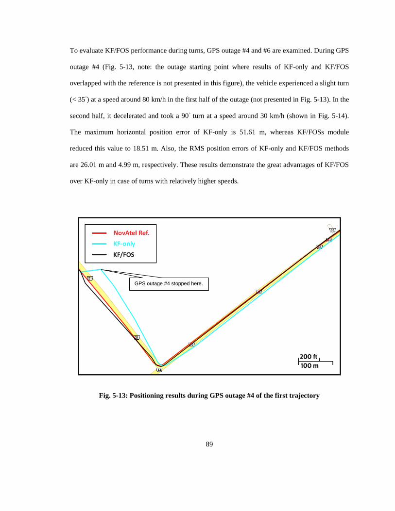
89

To evaluate KF/FOS performance during turns, GPS outage #4 and #6 are examined. During GPS

outage #4 (Fig. 5-13, note: the outage starting point where results of KF-only and KF/FOS

overlapped with the reference is not presented in this figure), the vehicle experienced a slight turn

(< 35◦) at a speed around 80 km/h in the first half of the outage (not presented in Fig. 5-13). In the

second half, it decelerated and took a 90◦ turn at a speed around 30 km/h (shown in Fig. 5-14).

The maximum horizontal position error of KF-only is 51.61 m, whereas KF/FOSs module

reduced this value to 18.51 m. Also, the RMS position errors of KF-only and KF/FOS methods

are 26.01 m and 4.99 m, respectively. These results demonstrate the great advantages of KF/FOS

over KF-only in case of turns with relatively higher speeds.

Fig. 5-13: Positioning results during GPS outage #4 of the first trajectory

GPS outage #4 stopped here.

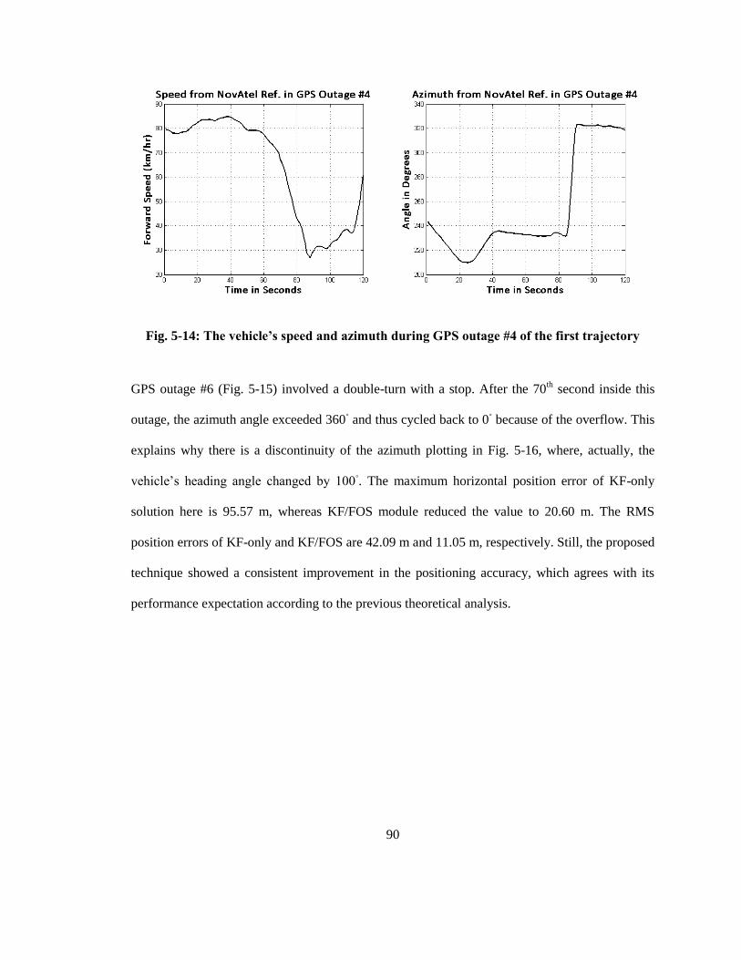
90

Fig. 5-14: The vehicle’s speed and azimuth during GPS outage #4 of the first trajectory

GPS outage #6 (Fig. 5-15) involved a double-turn with a stop. After the 70th second inside this

outage, the azimuth angle exceeded 360◦ and thus cycled back to 0

◦ because of the overflow. This

explains why there is a discontinuity of the azimuth plotting in Fig. 5-16, where, actually, the

vehicle’s heading angle changed by 100◦. The maximum horizontal position error of KF-only

solution here is 95.57 m, whereas KF/FOS module reduced the value to 20.60 m. The RMS

position errors of KF-only and KF/FOS are 42.09 m and 11.05 m, respectively. Still, the proposed

technique showed a consistent improvement in the positioning accuracy, which agrees with its

performance expectation according to the previous theoretical analysis.

91

Fig. 5-15: Positioning results in GPS outage #6 of the first trajectory


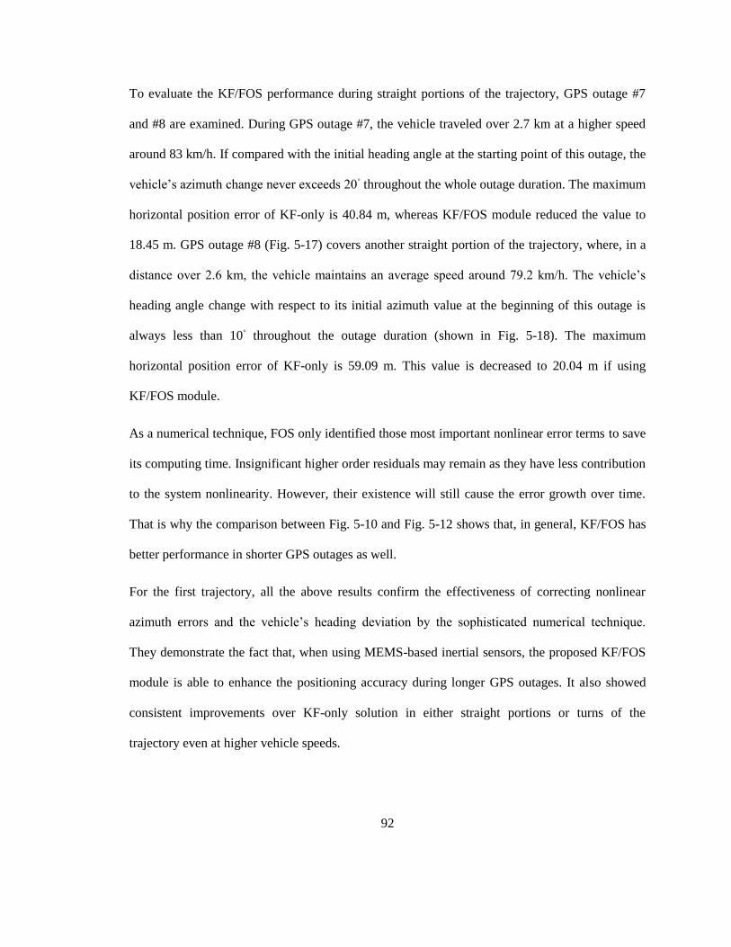
92

To evaluate the KF/FOS performance during straight portions of the trajectory, GPS outage #7

and #8 are examined. During GPS outage #7, the vehicle traveled over 2.7 km at a higher speed

around 83 km/h. If compared with the initial heading angle at the starting point of this outage, the

vehicle’s azimuth change never exceeds 20◦ throughout the whole outage duration. The maximum

horizontal position error of KF-only is 40.84 m, whereas KF/FOS module reduced the value to

18.45 m. GPS outage #8 (Fig. 5-17) covers another straight portion of the trajectory, where, in a

distance over 2.6 km, the vehicle maintains an average speed around 79.2 km/h. The vehicle’s

heading angle change with respect to its initial azimuth value at the beginning of this outage is

always less than 10◦ throughout the outage duration (shown in Fig. 5-18). The maximum

horizontal position error of KF-only is 59.09 m. This value is decreased to 20.04 m if using

KF/FOS module.

As a numerical technique, FOS only identified those most important nonlinear error terms to save

its computing time. Insignificant higher order residuals may remain as they have less contribution

to the system nonlinearity. However, their existence will still cause the error growth over time.

That is why the comparison between Fig. 5-10 and Fig. 5-12 shows that, in general, KF/FOS has

better performance in shorter GPS outages as well.

For the first trajectory, all the above results confirm the effectiveness of correcting nonlinear

azimuth errors and the vehicle’s heading deviation by the sophisticated numerical technique.

They demonstrate the fact that, when using MEMS-based inertial sensors, the proposed KF/FOS

module is able to enhance the positioning accuracy during longer GPS outages. It also showed

consistent improvements over KF-only solution in either straight portions or turns of the

trajectory even at higher vehicle speeds.

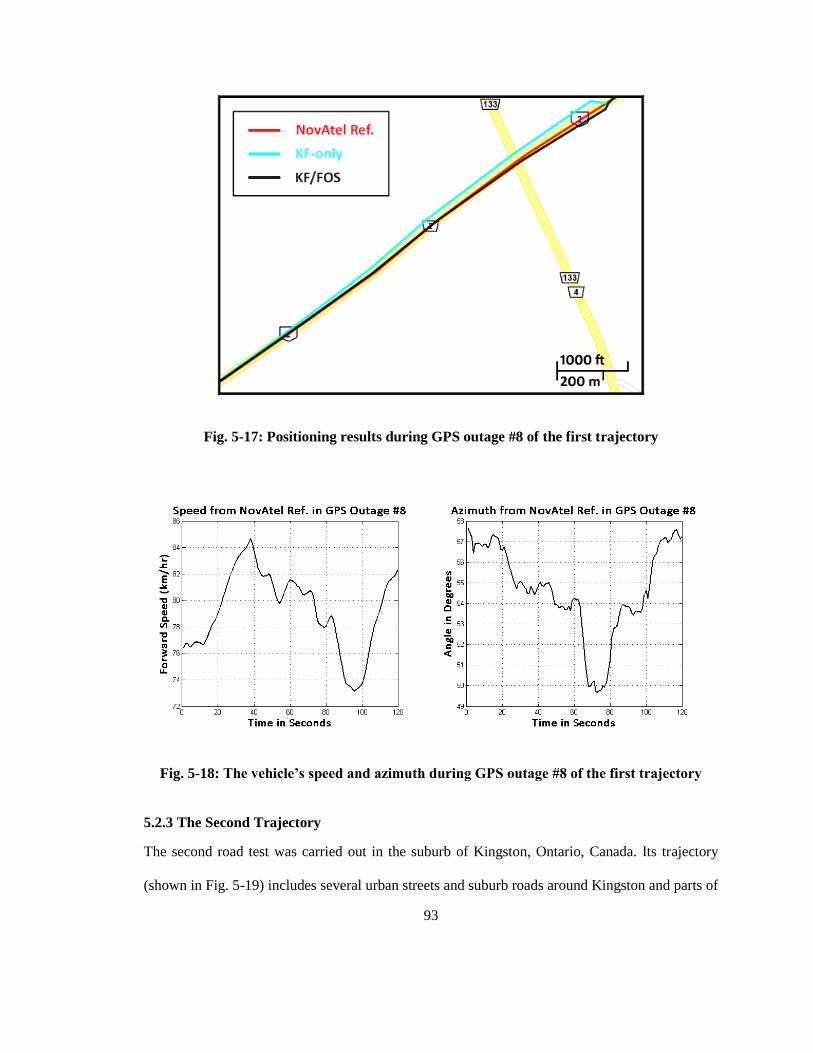
93

Fig. 5-17: Positioning results during GPS outage #8 of the first trajectory


5.2.3 The Second Trajectory

The second road test was carried out in the suburb of Kingston, Ontario, Canada. Its trajectory

(shown in Fig. 5-19) includes several urban streets and suburb roads around Kingston and parts of

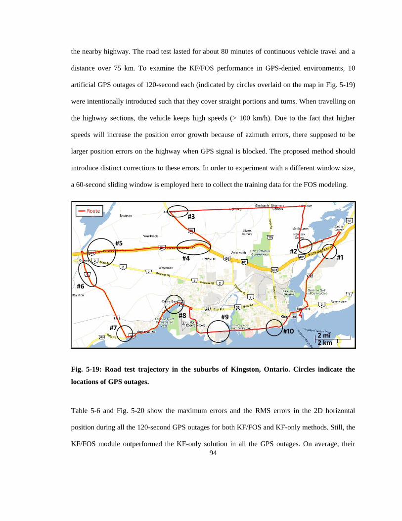
94

the nearby highway. The road test lasted for about 80 minutes of continuous vehicle travel and a

distance over 75 km. To examine the KF/FOS performance in GPS-denied environments, 10

artificial GPS outages of 120-second each (indicated by circles overlaid on the map in Fig. 5-19)

were intentionally introduced such that they cover straight portions and turns. When travelling on

the highway sections, the vehicle keeps high speeds (> 100 km/h). Due to the fact that higher

speeds will increase the position error growth because of azimuth errors, there supposed to be

larger position errors on the highway when GPS signal is blocked. The proposed method should

introduce distinct corrections to these errors. In order to experiment with a different window size,

a 60-second sliding window is employed here to collect the training data for the FOS modeling.

Fig. 5-19: Road test trajectory in the suburbs of Kingston, Ontario. Circles indicate the

locations of GPS outages.

Table 5-6 and Fig. 5-20 show the maximum errors and the RMS errors in the 2D horizontal

position during all the 120-second GPS outages for both KF/FOS and KF-only methods. Still, the

KF/FOS module outperformed the KF-only solution in all the GPS outages. On average, their

95

maximum position errors are 18.17 m and 64.03 m, respectively. The results of this trajectory are

consistent to those of the first trajectory. They proved the effectiveness of KF/FOS module again.

To evaluate the KF/FOS performance during sharp turns, GPS outage #2, #3, and #7 are

examined. In GPS outage #2, while decelerating from a speed around 80 km/h to a stop, the

vehicle conducted a 100◦ turn at an average speed of 67.1 km/h. In a distance over 2.23 km, the

maximum position errors of KF/FOS and KF-only methods are 27.00 m and 94.37 m,

respectively. The over 70% accuracy enhancement in position here shows the significance of

FOS-based reduction of nonlinear azimuth errors. This was confirmed once again in GPS outage

#7, where the vehicle experienced a 95◦ turn at an average speed over 60 km/h. In such a case, the

maximum position errors of KF/FOS and KF-only methods are 16.63 m and 37.64 m,

respectively. A more challenging situation took place in GPS outage #3 (Fig. 5-21). At a higher

average speed (> 73 km/h), the vehicle turned left by 130◦ in the last 20 seconds of the outage

(see Fig. 5-22). Nevertheless, the proposed method shows consistent advantages over KF-only by

decreasing the maximum position error from 52.32 m to 11.22 m.


outages in the second trajectory

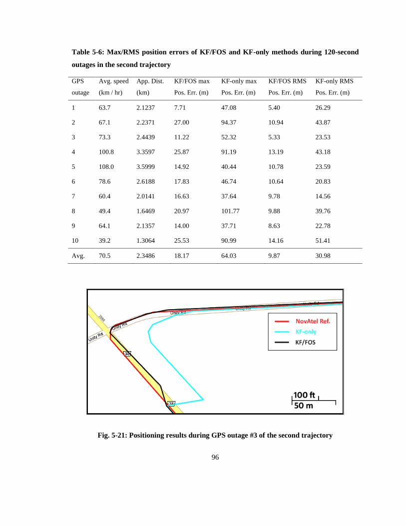
96


outages in the second trajectory

GPS

outage

Avg. speed

(km / hr)

App. Dist.

(km)

KF/FOS max

Pos. Err. (m)

KF-only max

Pos. Err. (m)

KF/FOS RMS

Pos. Err. (m)

KF-only RMS

Pos. Err. (m)

1 63.7 2.1237 7.71 47.08 5.40 26.29

2 67.1 2.2371 27.00 94.37 10.94 43.87

3 73.3 2.4439 11.22 52.32 5.33 23.53

4 100.8 3.3597 25.87 91.19 13.19 43.18

5 108.0 3.5999 14.92 40.44 10.78 23.59

6 78.6 2.6188 17.83 46.74 10.64 20.83

7 60.4 2.0141 16.63 37.64 9.78 14.56

8 49.4 1.6469 20.97 101.77 9.88 39.76

9 64.1 2.1357 14.00 37.71 8.63 22.78

10 39.2 1.3064 25.53 90.99 14.16 51.41

Avg. 70.5 2.3486 18.17 64.03 9.87 30.98

Fig. 5-21: Positioning results during GPS outage #3 of the second trajectory

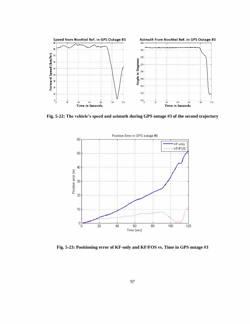
97

Fig. 5-22: The vehicle’s speed and azimuth during GPS outage #3 of the second trajectory

Fig. 5-23: Positioning error of KF-only and KF/FOS vs. Time in GPS outage #3

98

Fig. 5-23 depicts the positioning error of KF-only and KF/FOS module vs. time during GPS

outage #3 of the second trajectory. It shows that KF-only and KF/FOS had similar performance at

very beginning of the outage. Because of the growth of nonlinear azimuth errors, KF-only

positioning error increased quickly afterwards. The relatively high vehicle speed amplified the

procedure. At about the 100th second, the nonlinear azimuth error accumulated even faster during

the abrupt turning. On the other hand, thanks to the accurate nonlinear error prediction and

compensation provided by FOS, KF/FOS module was able to reduce the azimuth error drastically.

This, in turn, allowed it to introduce much better positioning accuracy than KF-only solution.

To evaluate the KF/FOS performance in case of high vehicle speeds, GPS outage #4 and #5 are

examined. For both of the outages, the average vehicle speed is greater than 100 km/h. During

GPS outage #4 (Fig. 5-24), the vehicle conducted 4 turns in succession: a 25◦ one around the 6

th

second, a 50◦ one around the 15

th second, a 65

◦ one around the 60

th second, and a 30

◦ one around

the 80th second (see Fig. 5-25). Magnified by high vehicle speeds, azimuth errors within the

above intensive orientation dynamics lead to greater position errors. The proposed KF/FOS

module further demonstrates its effectiveness in this outage by compensating for the nonlinear

azimuth errors. For instance, in a distance over 3.3 km, the maximum position error of KF-only

solution is 91.19 m, whereas KF/FOS module reduced the value to 25.87 m.

99

Fig. 5-24: Positioning results during GPS outage #4 of the second trajectory

Fig. 5-24 and Fig. 5-25 also show that the simulated GPS outage #4 happened when the vehicle

was accelerating to reach the highway. In such a case, during the modeling stage of KF/FOS

module, the nonlinear error model was constructed at lower vehicle speeds before reaching the

highway. However, this model can still provide accurate estimation of nonlinear azimuth errors in

the prediction stage with high vehicle speeds. On the other hand, in GPS outage #5, the vehicle

maintained high speeds (> 105 km/h) without intensive orientation changes at both of the training

and prediction stages. In a distance over 3.5 km, the maximum position error of KF-only is 40.44

m, whereas KF/FOS module reduced this value to 14.92 m. This reveals that FOS algorithm does

not require the system to maintain similar behavior between the modeling and prediction stages.

In fact, unlike AI algorithm such as the ANFIS module that learns local system dynamics with

fixed nonlinear structures, FOS approach identifies a dynamic model in a more flexible way. It is

open to update the model structure continuously using the most relevant candidate terms. Thus,

no matter the vehicle motion dynamics change greatly or not between the modeling and

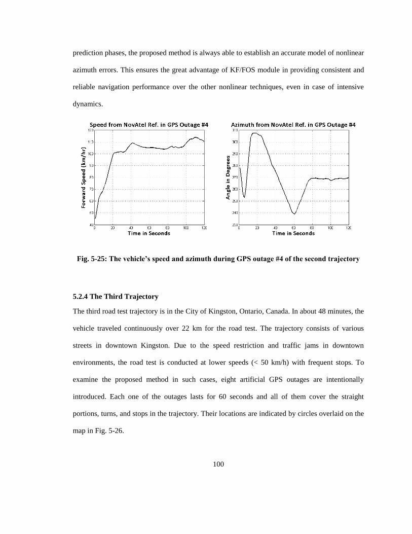
100

prediction phases, the proposed method is always able to establish an accurate model of nonlinear

azimuth errors. This ensures the great advantage of KF/FOS module in providing consistent and

reliable navigation performance over the other nonlinear techniques, even in case of intensive

dynamics.

Fig. 5-25: The vehicle’s speed and azimuth during GPS outage #4 of the second trajectory

5.2.4 The Third Trajectory

The third road test trajectory is in the City of Kingston, Ontario, Canada. In about 48 minutes, the

vehicle traveled continuously over 22 km for the road test. The trajectory consists of various

streets in downtown Kingston. Due to the speed restriction and traffic jams in downtown

environments, the road test is conducted at lower speeds (< 50 km/h) with frequent stops. To

examine the proposed method in such cases, eight artificial GPS outages are intentionally

introduced. Each one of the outages lasts for 60 seconds and all of them cover the straight

portions, turns, and stops in the trajectory. Their locations are indicated by circles overlaid on the

map in Fig. 5-26.

101

Fig. 5-26: Road test trajectory in downtown Kingston. Circles indicate the locations of GPS

outages.

The proposed method is applied on this trajectory by collecting the training data in a 60-second

sliding window. Table 5-7 and Fig. 5-27 show the maximum errors and the RMS errors in the 2D

horizontal position during all the 60-second GPS outages for both KF/FOS and KF-only solutions.

Clearly, the proposed KF/FOS module performs better than KF-only method in all the outages.

On average, the maximum position error of KF-only solution is 40.20 m. This value is decreased

by KF/FOS module to 14.04 m.

To evaluate the KF/FOS performance in case of low vehicle speeds with stops, GPS outage #2,

#3, and #8 are examined. In these outages, the vehicle speeds never exceeds 45 km/h and their

average value is less than 23 km/h. Furthermore, the vehicle stopped for at least one time during

each one of the above GPS outages. Over 60% positioning accuracy enhancement on average is

supplied by KF/FOS module with respect to the KF-only solution when the GPS signal is blocked.

The frequent stops result in vehicle dynamic changes between the training window and the

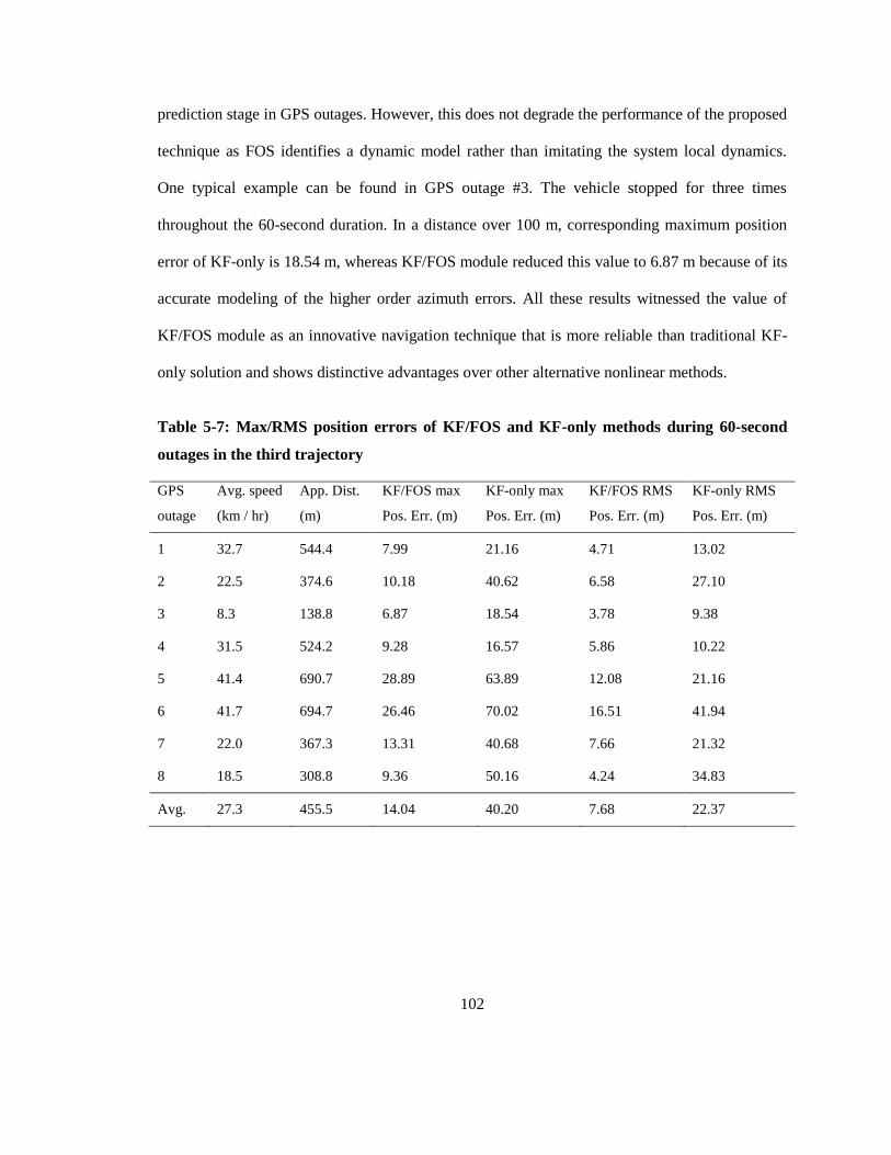
102

prediction stage in GPS outages. However, this does not degrade the performance of the proposed

technique as FOS identifies a dynamic model rather than imitating the system local dynamics.

One typical example can be found in GPS outage #3. The vehicle stopped for three times

throughout the 60-second duration. In a distance over 100 m, corresponding maximum position

error of KF-only is 18.54 m, whereas KF/FOS module reduced this value to 6.87 m because of its

accurate modeling of the higher order azimuth errors. All these results witnessed the value of

KF/FOS module as an innovative navigation technique that is more reliable than traditional KF-

only solution and shows distinctive advantages over other alternative nonlinear methods.


outages in the third trajectory

GPS

outage

Avg. speed

(km / hr)

App. Dist.

(m)

KF/FOS max

Pos. Err. (m)

KF-only max

Pos. Err. (m)

KF/FOS RMS

Pos. Err. (m)

KF-only RMS

Pos. Err. (m)

1 32.7 544.4 7.99 21.16 4.71 13.02

2 22.5 374.6 10.18 40.62 6.58 27.10

3 8.3 138.8 6.87 18.54 3.78 9.38

4 31.5 524.2 9.28 16.57 5.86 10.22

5 41.4 690.7 28.89 63.89 12.08 21.16

6 41.7 694.7 26.46 70.02 16.51 41.94

7 22.0 367.3 13.31 40.68 7.66 21.32

8 18.5 308.8 9.36 50.16 4.24 34.83

Avg. 27.3 455.5 14.04 40.20 7.68 22.37

103


outages in the third trajectory

5.3 Three Dimensional Vehicular Navigation using KF/FOS Module

Discussions in Chapter 3 presented the setup of 3D RISS. After adding extra sensors described in

subsection 5.3.1, the 2D RISS evolves into 3D RISS. KF/FOS module was applied on 3D RISS

as well to evaluate its effectiveness on enhancing the performance of three-dimensional vehicular

navigation. Two road test experiments in different scenarios were executed using the above

platform. Their trajectories were displayed and discussed in subsections 5.3.2 and 5.3.3.

Corresponding results demonstrated the great advantages of KF/FOS module over KF-only

solution on the positioning accuracy.

5.3.1 Experimental Setup of 3D RISS

A 3D RISS platform can be obtained by augmenting two extra accelerometers to the 2D RISS

used in subsection 5.2. As mentioned in subsection 3.1, the accelerometers are aligned along the

vehicle's forward and transversal directions, respectively. This setup makes them measure not

only the vehicle's acceleration on their sensing axes, but also gravity components caused by tilt

angles from the horizontal plane. By decoupling the gravity components and true vehicle

dynamics, readings of the extra accelerometers can be utilized in return to derive the vehicle's

104

pitch and roll using Eq (3.20). The pitch angle can then be used to calculate vertical velocities of

the vehicle in Eq (3.22). This further enables the calculation of vehicle's altitude. Consequently, a

full 3D solution to the vehicle navigation is achieved.

The 3D RISS used in this research consists of the 2D RISS used in subsection 5.2 and two extra

accelerometers offered by Crossbow IMU300CC-100 (Fig. 5-3). As a 6DOF MEMS-based IMU,

Crossbow IMU300CC-100 contains one accelerometer and one gyroscope per each axis of a 3D

Cartesian coordinate system. 2D RISS has made use of its vertical gyroscope only. Another two

accelerometers whose sensing axes are perpendicular to that of the vertical gyroscope are

employed in case of the 3D RISS. Still, the same NovAtel ProPack SPAN unit supplies the

reference solution to evaluate the proposed method on 3D RISS. Its built-in Honeywell HG1700

IMU (Fig. 5-5) has accelerometers with the same alignment as Crossbow IMU300CC-100. The

only difference lies in the fact that accelerometers in HG1700 IMU offer tactical grade

performance. Table 5-8 shows that they guarantee much better accuracy and reliability than their

MEMS-based competitors in Crossbow IMU300CC-100.

Table 5-8: Specifications of IMU 300CC-100 MEMS accelerometer and HG1700 tactical

grade accelerometer

Specifications IMU 300CC-100 accelerometer HG1700 accelerometer

Update rate > 100 Hz Up to 100 Hz

Dynamic range ± 2 g ± 50 g

Bias < 30 mg < 1.0 mg

Scale factor < 1% < 300 ppm

Velocity random walk < 0.15 m/s/ hr N/A

Linearity < 1 % < 500 ppm

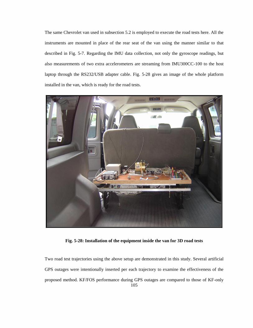
105

The same Chevrolet van used in subsection 5.2 is employed to execute the road tests here. All the

instruments are mounted in place of the rear seat of the van using the manner similar to that

described in Fig. 5-7. Regarding the IMU data collection, not only the gyroscope readings, but

also measurements of two extra accelerometers are streaming from IMU300CC-100 to the host

laptop through the RS232/USB adapter cable. Fig. 5-28 gives an image of the whole platform

installed in the van, which is ready for the road tests.

Fig. 5-28: Installation of the equipment inside the van for 3D road tests

Two road test trajectories using the above setup are demonstrated in this study. Several artificial

GPS outages were intentionally inserted per each trajectory to examine the effectiveness of the

proposed method. KF/FOS performance during GPS outages are compared to those of KF-only

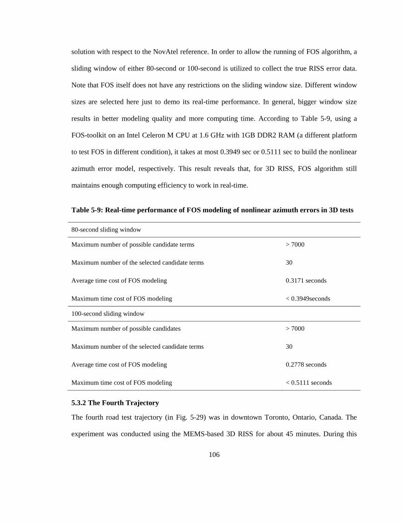
106

solution with respect to the NovAtel reference. In order to allow the running of FOS algorithm, a

sliding window of either 80-second or 100-second is utilized to collect the true RISS error data.

Note that FOS itself does not have any restrictions on the sliding window size. Different window

sizes are selected here just to demo its real-time performance. In general, bigger window size

results in better modeling quality and more computing time. According to Table 5-9, using a

FOS-toolkit on an Intel Celeron M CPU at 1.6 GHz with 1GB DDR2 RAM (a different platform

to test FOS in different condition), it takes at most 0.3949 sec or 0.5111 sec to build the nonlinear

azimuth error model, respectively. This result reveals that, for 3D RISS, FOS algorithm still

maintains enough computing efficiency to work in real-time.

Table 5-9: Real-time performance of FOS modeling of nonlinear azimuth errors in 3D tests


Maximum number of possible candidate terms > 7000



Maximum time cost of FOS modeling < 0.3949seconds


Maximum number of possible candidates > 7000




5.3.2 The Fourth Trajectory

The fourth road test trajectory (in Fig. 5-29) was in downtown Toronto, Ontario, Canada. The

experiment was conducted using the MEMS-based 3D RISS for about 45 minutes. During this

107

period, the testing vehicle had traveled in a distance over 18.6 km. The entire road test was

carried out on the urban streets at relatively lower vehicle speeds (23.3 km/h in average). The

intensive changes of the vehicle dynamics such as sudden accelerating, decelerating, and frequent

stops make this trajectory a challenging test for navigation algorithms. To examine the

performance of KF/FOS module in this downtown scenario, up to eight artificial GPS outages

were intentionally introduced such that they can simulate typical GPS-denied environments like

the urban canyons. Each one of these outages lasts for 60 seconds and they cover different

trajectory segments including straight portions and vehicle turnings. Circles overlaid on the map

in Fig. 5-29 present the location of these outages. To build the nonlinear azimuth error model at

the beginning of every outage, an 80-second sliding window is employed in this trajectory to

collect the training data required by FOS modeling.

Fig. 5-29: Road test trajectory in downtown Toronto. Circles indicate the locations of GPS

outages.

Fig. 5-30 and Table 5-10 display the maximum errors and RMS errors in position with respect to

NovAtel reference during all the 60-second GPS outages for both KF-only and KF/FOS methods.

108

The results confirmed that, for three-dimensional vehicular navigation using MEMS-based 3D

RISS, KF/FOS module performs better than KF-only solution on positioning accuracy in all the

outages. Specifically, the average value of KF-only maximum position errors exceeds 55 m.

KF/FOS module brought it down to 9.74 m, which introduced more than 82% improvement on

the overall performance.

GPS outage #1 of this trajectory gives a typical example to examine KF/FOS performance in case

of intensive 3D vehicle dynamics. During this outage (Fig. 5-31, both KF/FOS and KF-only

trajectory displays are synchronized with NovAtel reference according to the same GPS time), the

vehicle turned right by 125◦ in 12 seconds at first. This matter happened between the 6

th second

and 18th second of this outage, during which the vehicle decelerated from 25 km/h to 8 km/h and

restored afterwards. The second vehicle turning took place at the 28th second with a heading

angle change on right over 112◦. This procedure lasted for 10 seconds while the vehicle speed was

fluctuating between 37 km/h and 7 km/h. Fig. 5-32 illustrates details of the above horizontal

dynamics in terms of the NovAtel reference. The azimuth angle exceeded 360◦ and cycled back to

0◦ because of the overflow at the 57

th second of the outage. This caused the discontinuity of the

azimuth plotting in Fig. 5-32. Concerning the vertical vehicle dynamics, the changes of pitch and

roll from NovAtel reference provided useful information as shown in Fig. 5-33. The absolute

range of their changes can be up to 9.8◦ and 6.1

◦ in this outage, respectively. Specifically, during

the second vehicle turning, the pitch angle dropped from 2.45◦ to -5.52

◦. In parallel, the roll angle

swung between 4.39◦ and -1.67

◦ abruptly. Comparing to the other outages, this one witnessed the

most intensive vehicle dynamics on both the vertical direction and horizontal plane. In such a

case, the maximum position error of KF-only is 56.22 m, whereas KF/FOS module decreased this

value to 12.03 m. Moreover, the RMS position errors of KF-only and KF/FOS methods are 33.32

m and 8.78 m, respectively. These results are the solid proof to confirm the advantages of

109

KF/FOS module over KF-only approach on navigation performance and reliability, even when

encountering intensive 3D vehicle dynamics.


outages in the fourth trajectory


outages in the fourth trajectory

GPS

outage

Avg. speed

(km / hr)

App. Dist.

(m)

KF/FOS max

Pos. Err. (m)

KF-only max

Pos. Err. (m)

KF/FOS RMS

Pos. Err. (m)

KF-only RMS

Pos. Err. (m)

1 25.3 421.2 12.03 56.22 8.78 33.32

2 4.0 65.8 3.36 63.98 0.86 40.01

3 3.6 59.2 6.55 30.40 1.76 8.58

4 19.8 330.3 19.19 60.72 8.44 26.11

5 13.2 220.4 16.03 66.95 7.31 36.52

6 15.2 253.9 7.13 64.23 5.03 31.47

7 8.1 135.6 9.38 63.40 3.45 32.75

8 7.5 124.5 4.21 38.47 3.60 19.81

Avg. 12.1 201.4 9.74 55.55 4.90 28.57

110

Fig. 5-31: Positioning results during GPS outage #1 of the fourth trajectory

0 10 20 30 40 50 600

5

10

15

20

25

30

35

40

Speed from NovAtel Ref. in GPS Outage #1

Time in Seconds

Forw

ard

Sp

ee

d (

km/h

r)

0 10 20 30 40 50 600

50

100

150

200

250

300

350

400

Azimuth from NovAtel Ref. in GPS Outage #1

Time in Seconds

An

gle

in

De

gre

es

Fig. 5-32: The vehicle’s speed and azimuth during GPS outage #1 of the fourth trajectory

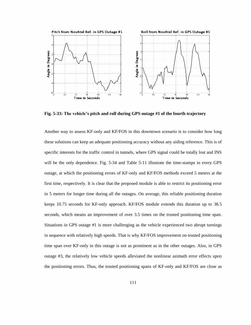
111

Fig. 5-33: The vehicle’s pitch and roll during GPS outage #1 of the fourth trajectory

Another way to assess KF-only and KF/FOS in this downtown scenario is to consider how long

these solutions can keep an adequate positioning accuracy without any aiding reference. This is of

specific interests for the traffic control in tunnels, where GPS signal could be totally lost and INS

will be the only dependence. Fig. 5-34 and Table 5-11 illustrate the time-stamps in every GPS

outage, at which the positioning errors of KF-only and KF/FOS methods exceed 5 meters at the

first time, respectively. It is clear that the proposed module is able to restrict its positioning error

in 5 meters for longer time during all the outages. On average, this reliable positioning duration

keeps 10.75 seconds for KF-only approach. KF/FOS module extends this duration up to 38.5

seconds, which means an improvement of over 3.5 times on the trusted positioning time span.

Situations in GPS outage #1 is more challenging as the vehicle experienced two abrupt turnings

in sequence with relatively high speeds. That is why KF/FOS improvement on trusted positioning

time span over KF-only in this outage is not as prominent as in the other outages. Also, in GPS

outage #3, the relatively low vehicle speeds alleviated the nonlinear azimuth error effects upon

the positioning errors. Thus, the trusted positioning spans of KF-only and KF/FOS are close as

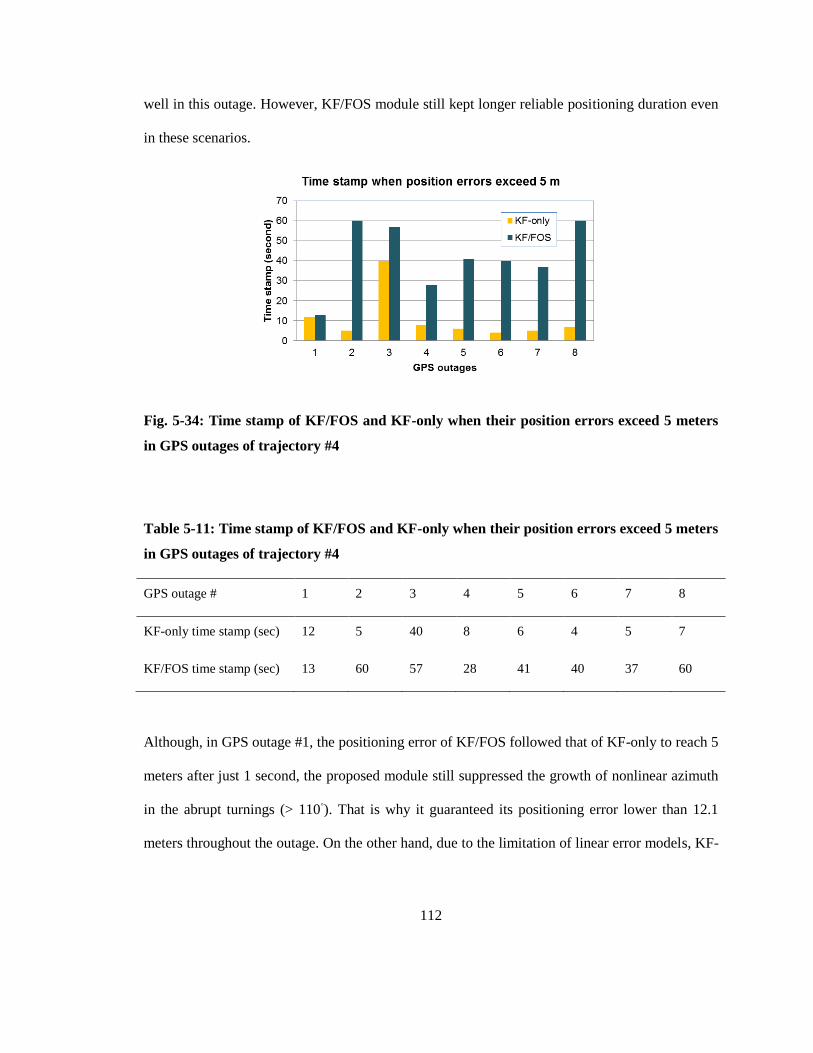
112

well in this outage. However, KF/FOS module still kept longer reliable positioning duration even

in these scenarios.

Fig. 5-34: Time stamp of KF/FOS and KF-only when their position errors exceed 5 meters

in GPS outages of trajectory #4

Table 5-11: Time stamp of KF/FOS and KF-only when their position errors exceed 5 meters

in GPS outages of trajectory #4

GPS outage # 1 2 3 4 5 6 7 8

KF-only time stamp (sec) 12 5 40 8 6 4 5 7

KF/FOS time stamp (sec) 13 60 57 28 41 40 37 60

Although, in GPS outage #1, the positioning error of KF/FOS followed that of KF-only to reach 5

meters after just 1 second, the proposed module still suppressed the growth of nonlinear azimuth

in the abrupt turnings (> 110◦). That is why it guaranteed its positioning error lower than 12.1

meters throughout the outage. On the other hand, due to the limitation of linear error models, KF-

113

only approach cannot compensate the higher order RISS errors, thus yielding larger positioning

errors up to 56.2 meters eventually.

In the assessment of more general cases, the best results of KF/FOS module were discovered in

the second and the last GPS outages where its positioning error kept lower than 5 meters

throughout the entire 60-second duration. Contrarily, during the second and the last GPS outage,

the positioning error of KF-only solution is beyond 5 meters after just 5 and 7 seconds,

respectively, in the same condition. The above comparison demonstrates the apparent advantage

of KF/FOS over KF-only on bridging frequent short-term GPS outages, which are very common

in the urban areas.

5.3.3 The Fifth Trajectory

The fifth trajectory was obtained during a trip from City of Kingston to Jones Falls, Ontario,

Canada. The road test lasted for about 50 minutes of continuous vehicle travel with a distance

over 56 km. The trajectory covers several urban streets and a plenty of suburb roads. To examine

the proposed technique in this road test, 6 artificial GPS outages were intentionally introduced

with the duration of 120 seconds per each. Their locations are highlighted by circles overlaid on

Fig. 5-35. During these outages, the testing vehicle experienced situations including straight

portions, frequent turns, higher speeds, lower speeds with stops, and the mixture of them.

A 100-second sliding window is employed to collect the training data for FOS modeling of

nonlinear azimuth errors. Table 5-12 and Fig. 5-36 present the maximum and RMS position

errors during all the 120-second GPS outages for both KF-only and KF/FOS solutions. Still, the

proposed method performs better than KF-only approach in every outage of this trajectory. For

instance, on average, the maximum position error of KF-only solution is greater than 75 meters.

114

KF/FOS module reduced the value to 27.8 meters, thus introducing a 63% enhancement on the

overall positioning accuracy.

Without the speed restriction and traffic jams as seen in the third and the fourth trajectories, the

testing vehicle traveled faster in this trajectory. Its average speed was greater than 60 km/h. To

evaluate KF/FOS performance in case of sharp turns with relatively higher speeds, GPS outage

#4 is studied.

Fig. 5-35: Road test trajectory from Kingston to Jones Falls, Ontario, Canada. Circles

indicate the locations of GPS outages.

115

Fig. 5-37 shows that, in a distance over 1.1 km, the testing vehicle experienced two turns in

sequence: a 48◦ one at the 17

th second and a 95

◦ one at the 49

th second. If compared with the other

GPS outages in this trajectory, the situation here is more challenging because of the rapid vehicle

dynamics. For instance, in the second turning, the vehicle took only 7 seconds to complete an

orientation change over 90◦ at a speed around 20 km/h. Moreover, abrupt deceleration and

acceleration can be found in between of the two turnings. In such a scenario, the maximum

position error of KF-only solution reached 120 meters. Owing to its tolerance of various short-

term noise and random sensor errors, KF/FOS module is able to update the nonlinear model

continuously by fitting the behavior of true azimuth errors. This feature ensures its reliable error

predictions and helps it to introduce more than 78% accuracy enhancement over KF-only solution

by decreasing the position error to 25.5 meters. The above results and analysis confirmed the

advantages of KF/FOS module on offering consistent improvement in 3D vehicle navigation.

This enhancement maintained even in challenging situations such as abrupt turnings with higher

vehicle speeds.


outages in the fifth trajectory

GPS

outage

Avg. speed

(km / hr)

App. Dist.

(km)

KF/FOS max

Pos. Err. (m)

KF-only max

Pos. Err. (m)

KF/FOS RMS

Pos. Err. (m)

KF-only RMS

Pos. Err. (m)

1 85.3 2.8441 8.34 26.85 5.40 16.51

2 88.1 2.9359 31.30 75.76 20.60 58.55

3 85.1 2.8364 32.14 48.65 18.20 27.50

4 34.5 1.1496 25.49 120.43 18.68 69.27

5 71.4 2.3815 29.27 115.45 18.19 66.39

6 76.7 2.5552 39.91 68.43 20.32 28.16

Avg. 73.5 2.4504 27.74 75.93 16.90 44.40

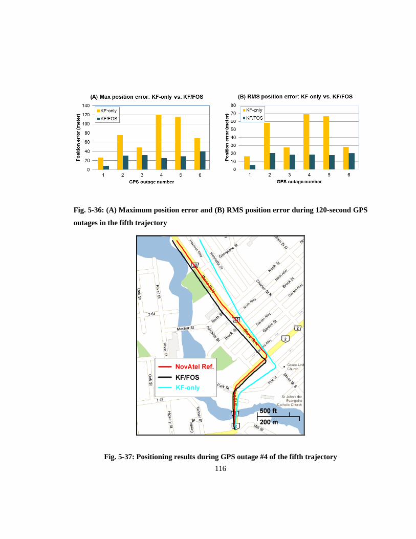
116


outages in the fifth trajectory

Fig. 5-37: Positioning results during GPS outage #4 of the fifth trajectory

117

By selecting candidate functions in terms of the model-fit m.s.e. reduction, FOS can always

detect the most significant error terms as well as their weights. Thus, even using a short range of

training data, it is still able to best-fit RISS error dynamics without any a priori knowledge about

the system. If compared with the other nonlinear modeling methods like ANFIS, FOS does not

mimic nonlinear system dynamics. It identifies higher order error terms as a mathematical model

according to their contribution to system nonlinearity and uses them to update the structure of

nonlinear models online. As a result, the prediction of FOS model keeps stable accuracy even if

the dynamic behavior of the vehicle varies between the modeling and prediction stages. On the

other hand, ANFIS method learns the knowledge of nonlinear system from the local training data.

Thus, its performance highly relies on the consistency of the training data. Any change of the

local error statistics is very common for MEMS device but will undermine reliability of AI

training and prediction quality. This explains why AI approach performs well in GPS outages of

shorter time (< 45 sec) [10] while FOS can offer the same or better positioning accuracy in GPS

outages of longer duration. Moreover, due to its tolerance to non-stationary stochastic sensor

error, FOS has proven itself adept at removing both colored and white noise from the system

errors, which cannot be fully achieved by KF alone. This introduces great advantages when

processing IMU measurements corrupted by MEMS sensor errors.

In addition, the prompt responds of KF/FOS module shown in this chapter and Chapter 7

illustrates that FOS is able to offer adequate real-time performance for the online vehicle

navigation. In contrast, the high computing complexity of the other nonlinear methods like AI

(NN, ANFIS, etc.) prevents their utilization in the real life. For instance, as mentioned in

subsection 5.2.1, it will take seconds (or even minutes in extreme cases) for ANFIS to do the

same job as FOS when working on the same trajectory data used in this chapter. That is why they

are restricted in the post-processing of vehicle applications.

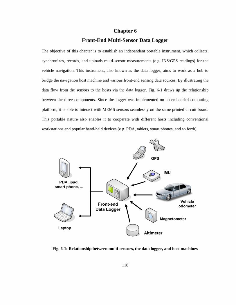
118

Chapter 6

Front-End Multi-Sensor Data Logger

The objective of this chapter is to establish an independent portable instrument, which collects,

synchronizes, records, and uploads multi-sensor measurements (e.g. INS/GPS readings) for the

vehicle navigation. This instrument, also known as the data logger, aims to work as a hub to

bridge the navigation host machine and various front-end sensing data sources. By illustrating the

data flow from the sensors to the hosts via the data logger, Fig. 6-1 draws up the relationship

between the three components. Since the logger was implemented on an embedded computing

platform, it is able to interact with MEMS sensors seamlessly on the same printed circuit board.

This portable nature also enables it to cooperate with different hosts including conventional

workstations and popular hand-held devices (e.g. PDA, tablets, smart phones, and so forth).

Fig. 6-1: Relationship between multi-sensors, the data logger, and host machines

Altimeter

119

The following sections cover the hardware description, firmware / software design, and

experiment results of this data logger.

6.1 Hardware Description

In this study, the data logger is comprised of a GPS receiver chipset, a MEMS grade IMU, a

digital compass, an altimeter, a SD card slot, a Reduced Instruction Set Computing (RISC)

microcontroller, a communication port interfacing OBD-II scan tools, and an uploading channel

to the host. As shown in Fig. 6-2, the microcontroller plays a role of the central unit to control all

the peripheral sensors and collect their measurements via different bus systems. After

synchronizing the collected results, the microcontroller can either upload them to the host

machine or save them into the SD card for post-processing. To accommodate the mobile

environment, all the modules inside the shadow area of Fig. 6-2 are assembled on a printed circuit

board, which can be easily mounted to vehicles.

Cortex-M3RISC CPU@72 MHz

LEA-5T/6TGPS Receiver

ADIS IMU:16405 / 16385

HMC5883Digital compass

MS5803Altimeter

SD cardstorage

HOST:Server, PC, PDA, Smartphone, …

UART2

UART1

SDIO

I2C

I2C

SPI

Front-End Multi-Sensor Data Logger

OBD-IIScan tool

UART3

Fig. 6-2: Block diagram of the front-end multi-sensor data logger

120

6.1.1 Ublox GPS Receiver Chipset

The data logger's GPS receiver chipset is a product from Ublox. Its part number is LEA-5T. A

pin-compatible alternative is LEA-6T. Both LEA-5T and LEA-6T supply GPS/GALILEO dual

service, GPS raw data, and precision timing at an accuracy of up to 15 ns according to their

datasheets. Comparing to other GPS receivers, Ublox LEA-5T/6T has smaller size (22.4 mm

17.0 mm 3.0 mm), lower cost (< US$ 200), and lower power consumption (2.7 V – 3.6V, <

150 mA). These advantages make them very suitable for vehicle navigation. Performance reports

in Table 6-1 illustrate that LEA-5T and 6T are strong competitors of those high-end products.

Table 6-1: Ublox LEA-5 GPS Performance [79]

Parameter Specification

Receiver Type

50 Channels

GPS L1 frequency – C/A code

GALILEO Open Service L1 frequency

Time-To-First-Fix

Cold Start (Autonomous) 29 s

Warm Start (Autonomous) 29 s

Hot Start (Autonomous) < 1 s

Aided Start < 1 s

Sensitivity

Tracking & Navigation -160 dBm

Reacquisition -160 dBm

Cold Start (Autonomous) -144 dBm

Horizontal Position Accuracy Autonomous < 2.5 m

SBAS < 2.0 m

Accuracy of Time Pulse Signal

RMS 30 ns

99% < 60 ns

Compensated (LEA-5T) 15 ns

Time Pulse Configurable: 0.25 – 999 Hz

Max Navigation Update Rate 4 Hz

Velocity Accuracy 0.1 m/s

Heading Accuracy 0.5 degrees

121

If compared to other low cost chipsets, LEA-5T and 6T offer up to 50 satellite channels and A-

GPS supports to ensure better positioning accuracy and shorter Time-To-First-Fix (TTFF).

Meanwhile, its GPS raw data outputs allow the tightly coupled INS/GPS integration, which is

impossible for the other low cost GPS receiver ICs (< $100). Also, there are two communication

protocols in Ublox chipsets: standard NMEA (ASCII) and proprietary UBX (binary). This

flexibility gives users the freedom to adjust their choice in general positioning or specific fields.

For example, this research requires LEA-5T/6T to output its data in UBX format so that the

logger can collect long-byte GPS packets such as satellite pseudo-ranges and ephemeris more

efficiently. Although LEA-5T/6T supports various digital interfaces, in this study, it

communicates with the microcontroller via the UART.

6.1.2 MEMS Grade IMU from Analog Devices

The inertial sensor used by the data logger is a MEMS grade product from Analog Devices. Its

part number is ADIS16385. A pin-compatible alternative is ADIS16405. Both are 6DOF full

IMU with 3-Axis accelerometers and gyroscopes. ADIS16405 has an extra built-in Tri-Axis

magnetometer (equivalent to digital compass). After receiving their outputs, the data logger can

select readings of only Z-axis gyroscope and X/Y-axis accelerometers to build the RISS

introduced in Chapter Three. Alternatively, to reduce the system cost further, the full IMU can be

replaced by the other pin-compatible modules with only single-axis gyroscope (e.g. ADIS16300).

ADIS16385 and ADIS16405 share the common advantages of MEMS device: small size, light

weight (16 – 59 grams), low power consumption (5V, 70 – 132 mA), and relatively low cost

(US$ 400 – 900). Fig. 6-3 and Fig. 6-4 show the small cubic package of ADIS16385 and

ADIS16405, respectively. Their performance is listed in Table 6-2. Obviously, these IMUs are

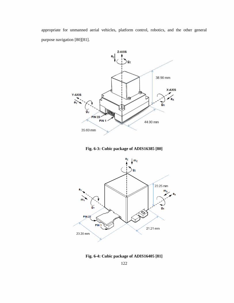
122

appropriate for unmanned aerial vehicles, platform control, robotics, and the other general

purpose navigation [80][81].

Fig. 6-3: Cubic package of ADIS16385 [80]

Fig. 6-4: Cubic package of ADIS16405 [81]

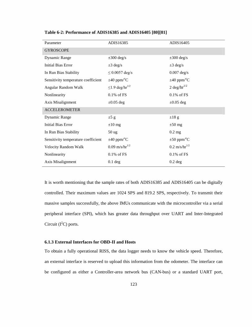
123

Table 6-2: Performance of ADIS16385 and ADIS16405 [80][81]

Parameter ADIS16385 ADIS16405

GYROSCOPE

Dynamic Range ±300 deg/s ±300 deg/s

Initial Bias Error ±3 deg/s ±3 deg/s

In Run Bias Stability ≤ 0.0057 deg/s 0.007 deg/s

Sensitivity temperature coefficient ±40 ppm/oC ±40 ppm/

oC

Angular Random Walk ≤1.9 deg/hr1/2

2 deg/hr1/2

Nonlinearity 0.1% of FS 0.1% of FS

Axis Misalignment ±0.05 deg ±0.05 deg

ACCELEROMETER

Dynamic Range ±5 g ±18 g

Initial Bias Error ±10 mg ±50 mg

In Run Bias Stability 50 ug 0.2 mg

Sensitivity temperature coefficient ±40 ppm/oC ±50 ppm/

oC

Velocity Random Walk 0.09 m/s/hr1/2

0.2 m/s/hr1/2

Nonlinearity 0.1% of FS 0.1% of FS

Axis Misalignment 0.1 deg 0.2 deg

It is worth mentioning that the sample rates of both ADIS16385 and ADIS16405 can be digitally

controlled. Their maximum values are 1024 SPS and 819.2 SPS, respectively. To transmit their

massive samples successfully, the above IMUs communicate with the microcontroller via a serial

peripheral interface (SPI), which has greater data throughput over UART and Inter-Integrated

Circuit (I2C) ports.

6.1.3 External Interfaces for OBD-II and Hosts

To obtain a fully operational RISS, the data logger needs to know the vehicle speed. Therefore,

an external interface is reserved to upload this information from the odometer. The interface can

be configured as either a Controller-area network bus (CAN-bus) or a standard UART port,

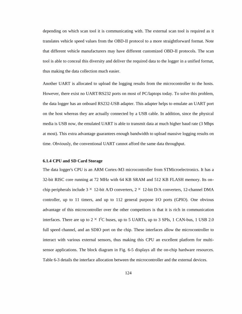
124

depending on which scan tool it is communicating with. The external scan tool is required as it

translates vehicle speed values from the OBD-II protocol to a more straightforward format. Note

that different vehicle manufacturers may have different customized OBD-II protocols. The scan

tool is able to conceal this diversity and deliver the required data to the logger in a unified format,

thus making the data collection much easier.

Another UART is allocated to upload the logging results from the microcontroller to the hosts.

However, there exist no UART/RS232 ports on most of PC/laptops today. To solve this problem,

the data logger has an onboard RS232-USB adapter. This adapter helps to emulate an UART port

on the host whereas they are actually connected by a USB cable. In addition, since the physical

media is USB now, the emulated UART is able to transmit data at much higher baud rate (3 Mbps

at most). This extra advantage guarantees enough bandwidth to upload massive logging results on

time. Obviously, the conventional UART cannot afford the same data throughput.

6.1.4 CPU and SD Card Storage

The data logger's CPU is an ARM Cortex-M3 microcontroller from STMicroelectronics. It has a

32-bit RISC core running at 72 MHz with 64 KB SRAM and 512 KB FLASH memory. Its on-

chip peripherals include 3 12-bit A/D converters, 2 12-bit D/A converters, 12-channel DMA

controller, up to 11 timers, and up to 112 general purpose I/O ports (GPIO). One obvious

advantage of this microcontroller over the other competitors is that it is rich in communication

interfaces. There are up to 2 I2C buses, up to 5 UARTs, up to 3 SPIs, 1 CAN-bus, 1 USB 2.0

full speed channel, and an SDIO port on the chip. These interfaces allow the microcontroller to

interact with various external sensors, thus making this CPU an excellent platform for multi-

sensor applications. The block diagram in Fig. 6-5 displays all the on-chip hardware resources.

Table 6-3 details the interface allocation between the microcontroller and the external devices.

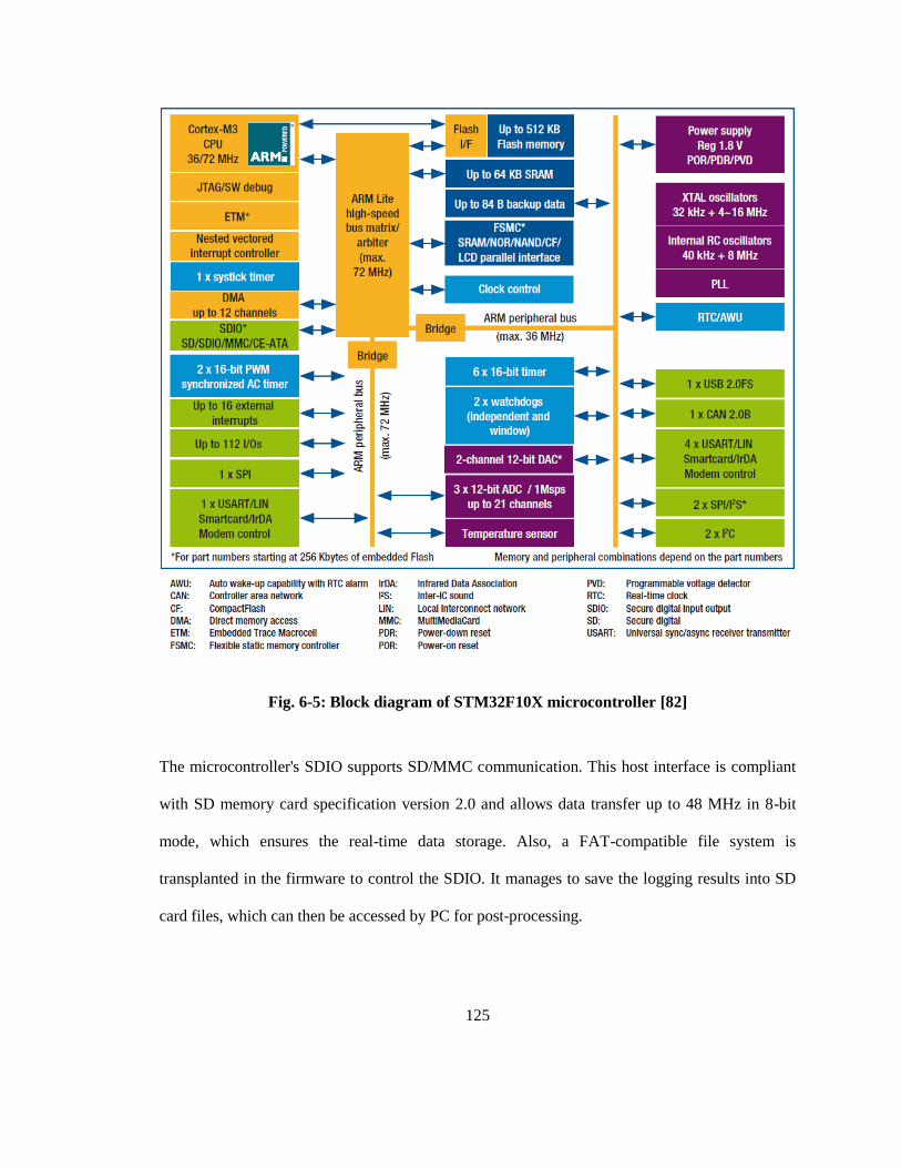
125

Fig. 6-5: Block diagram of STM32F10X microcontroller [82]

The microcontroller's SDIO supports SD/MMC communication. This host interface is compliant

with SD memory card specification version 2.0 and allows data transfer up to 48 MHz in 8-bit

mode, which ensures the real-time data storage. Also, a FAT-compatible file system is

transplanted in the firmware to control the SDIO. It manages to save the logging results into SD

card files, which can then be accessed by PC for post-processing.

126

Table 6-3: Allocation of STM32 communication interfaces for external devices

Devices Allocation of STM32 communication interfaces

Ublox GPS receiver chipset UART-2

OBD-II scan tool UART-3

Host machine (PC, laptop, PDA, etc.) UART-1

IMU ADIS16385/ADIS16405 SPI-2

Digital Compass HMC5883 I2C-2

Altimeter MS5803 I2C-2

SD card SDIO

6.2 Firmware / Software Design

The data logger needs its firmware to drive the hardware and manipulate the logging routine. The

firmware design relies on the driver program of each sensor and a scheduler that administrates the

multi-sensor logging tasks. The latter is more challenging as it is in charge of keeping all the

parallel tasks away from any conflicts in time and resource. Meanwhile, the scheduler also needs

to synchronize the logging results from different sensors and generate corresponding timing

information (time tag) correctly for INS mechanization. Therefore, the scheduler is the kernel of

the firmware design. Other than data collection, formatted packets are required as well to upload

the logging results to the hosts. A dedicated protocol is developed for it. On the host side, this

research designed PC-based software to receive and visualize the logging results from the logger.

6.2.1 Multi-Task Scheduling and Synchronization

The data logger’s parallel tasks involve GPS data logging, IMU data logging, OBD-II data

logging, compass / altimeter data logging, DMA-based sensor / GPS data uploading, and sensor /

GPS data storage on the SD card. Each task should be granted an appropriate priority so that the

127

scheduler can have a criterion to manage them. In this design, there are three priority levels: ultra-

high priority, high priority, and medium priority.

Comparing to the other tasks, GPS data logging is particular. Firstly, it is the Ublox chipset, not

the microcontroller, who initiates the data transfer. Thus, the CPU needs to response GPS data

receiving promptly at any time as it has no idea when the transmission will take place. Secondly,

the GPS receiver has a larger packet size than any other sensor alone. This makes GPS data

logging more susceptible to suffer missing bytes if it can be interrupted or blocked by the other

tasks. Due to the above concerns, GPS data logging occupied the ultra-high priority exclusively.

Since the microcontroller has the full control of all the sensors, it can depend on its built-in timer

to dispatch the logging task of every sensor in sequence. This helps to avoid any time conflicts

between the multi-sensor logging. The built-in timer also has the flexibility to trigger each sensor

logging according to its own sample rate. For example, the 100-Hz IMU data logging is initiated

right after the 1-Hz OBD-II data polling with latency in dozens of nanoseconds. Since there exist

no time overlaps between each other, all sensor logging tasks can share the high priority.

As a single-core CPU, the ST microcontroller is exclusively occupied by one task at one time.

Fortunately, the on-chip DMA channel allows the sensor / GPS data uploading in background

process when the CPU is busy on data collection. Similarly, the SD card storage of sensor / GPS

data should not delay or interrupt any concurrent data logging tasks. Thus, the data uploading and

storage tasks share the medium priority.

After granting priorities to tasks, the data logger still requires a mechanism to arbitrate behaviors

of concurrent tasks. This job was handled by the nested vectored interrupt controller (NVIC)

inside the CPU successfully. NVIC guarantees that a task can be interrupted if and only if another

task with higher priority is activated while its execution. Before branching to another task, NVIC

128

automatically saves the context of the interrupted task into stack. Once the task with higher

priority is done, it restores the context from stack and allows the CPU to continue the interrupted

task. The design ensures the latency of context switch and execution of tasks with higher priority

is always in the acceptable range of the task being interrupted. Consequently, all the tasks can

coexist and cooperate on the same CPU.

According to [83], ST microcontroller’s NVIC supports nested interrupts with up to 16 priority

levels, which are quite enough for this design. Fig. 6-6 illustrates the prioritization of all the tasks

and NVIC management upon them.

Nested Vectored Interrupt Controller (NVIC)

GPS Data Logging

IMU Data Logging

OBD-II Data Logging

Compass Data Logging

Altimeter Data Logging

DMA-Based Sensor Data uploading

DMA-Based GPS Data uploading

Sensor / GPS Data storage on SD card

Ultra-high priority

High priority

Medium priority

Fig. 6-6: Prioritization and NVIC management of data logger’s tasks

As mentioned before, one advantage of INS over GPS is its higher sample rate. In this study, the

data logger collects IMU data at a sample rate around 100 SPS whereas Ublox chipset offers GPS

129

updates at 1 Hz. Other sensor readings have different sample rates as well (OBD-II polling - 1 Hz,

compass / altimeter - 25 Hz). How to synchronize these logging results is another focus of the

scheduler. This function is also crucial for INS mechanization as its running needs correct timing

information of inertial sensor measurements.

At present, almost all GPS receivers provide pulse-per-second (PPS) signal. PPS accuracy is

reliable since GPS is a reference not only for positioning, but also for timing. Specifically, the

periodic PPS of on-board Ublox chipset has a precision up to 15 ns, which is way shorter than the

duration between two consecutive IMU, GPS, and OBD-II updates. Thus, the data logger can

benefit from the PPS output to synchronize the logging and uploading tasks as shown in Fig. 6-7.

PPS

GPS DataReceiving

IMU DataSampling

OBD-II Polling

IMU / OBD-IIData Upload

GPS DataUpload

Fig. 6-7: Synchronization of logging and uploading tasks

The idea is to use PPS signal as the starting point of data logging and uploading for every second.

Typically, the latency between Ublox PPS and its GPS update is about 100 ms. Data logger will

130

start IMU data logging once it detects the PPS. This task will keep on working between every two

consecutive PPS signals and, thus, ensure the continuous data collection. OBD-II polling will be

triggered by the end of every second (about 10 ms before the next PPS) in order to avoid being

blocked by tasks with higher priority (e.g. GPS data receiving). However, since the first OBD-II

polling (Speed#2) is very close to the second PPS signal (PPS#2) in Fig. 6-7, the current OBD-II

data are always classified as logging results synchronized with the next PPS. In parallel, when the

CPU detects the PPS, it will initiate DMA-based data uploading as well. Since the IMU logging

lasts for the entire second, its current data can only be uploaded after the next PPS. In contrast,

the current OBD-II reading and GPS updates can be shipped immediately in the same second.

The host has the ability to distinguish this difference according to the timing information

mentioned below.

To let the host be aware of synchronization results and perform INS mechanization afterwards,

the data logger needs to generate a time stamp for every logging sample. This procedure is also

known as time tagging. Its reference is provided by the microcontroller's 24-bit system tick timer.

This timer is reset by every PPS signal. It automatically counts at a frequency up to 9 MHz, thus

ensuring an accuracy of 0.111 microseconds. The CPU queries its counter at the exact moment

when a logging sample is acknowledged. The counter's value will be buffered together with its

corresponding sample as the logging results ready for uploading. Eventually, the absolute time

tag of every logging sample T can be determined by Eq. (6.1), where GPST denotes GPS week

time in milliseconds (timing baseline), tickT refers to the timing results of the system tick timer

since the last PPS (timing offset), N is the original counter value.

0.1 1, 1GPS tick G ccPST T TT N T T s (6.1)

131

In summary, the data logger’s scheduler relies on a priority system controlled by NVIC, the PPS

signal from the GPS receiver, and the system tick timer to manage, synchronize, and time-stamp

the data logging.

6.2.2 Protocol Design of the Unified Uploading Packet

There are several reasons of designing unified uploading packets for the data logger.

1. The system needs a well-defined data structure to buffer the logging results safely and

efficiently.

2. Digital devices depend on predefined protocols to understand each other during their

communication. The data logger and its host require the same mechanism to regulate

their behaviors when the logging results are transmitted between them.

3. The SD card file needs a data structure to organize its storage of logging results in a

consistent format.

4. The unified uploading packets simplify the interface between the data logger and its host.

No matter from which sensor the data logger collects data, it always deliver its logging

results in the same format. This helps the host to focus on running navigation algorithm

rather than caring about data collection details. Also, because of the unified packet, no

changes are needed on the host even if the data logger has extra sensor readings in the

future enhancement.

5. Necessary fields inside the formatted packet reflect the uploading quality and tell whether

the packet is valid. They are very helpful in the communication diagnosis and

troubleshooting.

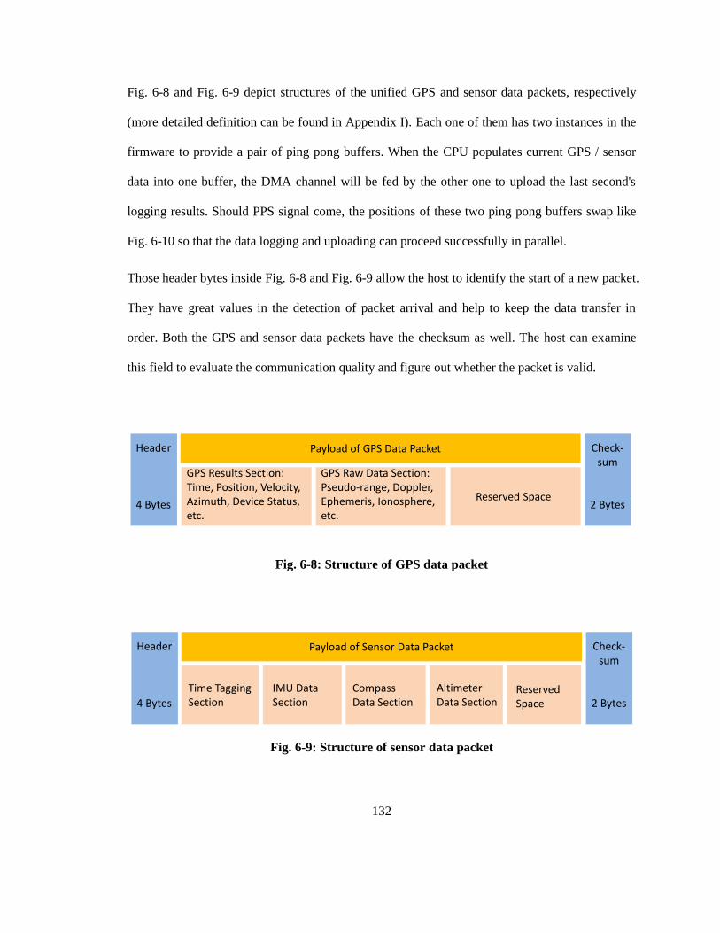
132

Fig. 6-8 and Fig. 6-9 depict structures of the unified GPS and sensor data packets, respectively

(more detailed definition can be found in Appendix I). Each one of them has two instances in the

firmware to provide a pair of ping pong buffers. When the CPU populates current GPS / sensor

data into one buffer, the DMA channel will be fed by the other one to upload the last second's

logging results. Should PPS signal come, the positions of these two ping pong buffers swap like

Fig. 6-10 so that the data logging and uploading can proceed successfully in parallel.

Those header bytes inside Fig. 6-8 and Fig. 6-9 allow the host to identify the start of a new packet.

They have great values in the detection of packet arrival and help to keep the data transfer in

order. Both the GPS and sensor data packets have the checksum as well. The host can examine

this field to evaluate the communication quality and figure out whether the packet is valid.

Header

4 Bytes

Payload of GPS Data Packet

GPS Results Section:Time, Position, Velocity,Azimuth, Device Status,etc.

GPS Raw Data Section:Pseudo-range, Doppler,Ephemeris, Ionosphere,etc.

Reserved Space

Check-sum

2 Bytes

Header

4 Bytes

Payload of Sensor Data Packet

Time TaggingSection

Check-sum

2 Bytes

IMU DataSection

Compass Data Section

Altimeter Data Section

Reserved Space

Fig. 6-8: Structure of GPS data packet

Header

4 Bytes

Payload of GPS Data Packet

GPS Results Section:Time, Position, Velocity,Azimuth, Device Status,etc.

GPS Raw Data Section:Pseudo-range, Doppler,Ephemeris, Ionosphere,etc.

Reserved Space

Check-sum

2 Bytes

Header

4 Bytes

Payload of Sensor Data Packet

Time TaggingSection

Check-sum

2 Bytes

IMU DataSection

Compass Data Section

Altimeter Data Section

Reserved Space

Fig. 6-9: Structure of sensor data packet

133

Buffer A

Buffer A

Buffer A

Buffer B

Buffer B

Buffer B

PPS PPS

μController

Host upload datafrom the buffer

store datainto the buffer

Timeline

Timeline

Fig. 6-10: Ping pong buffers and their swap

6.2.3 Host Software

The host software was developed on the PC platform. Its basic objective is receiving packets sent

by the data logger and saving the logging results into a binary file. To monitor this procedure, the

host software visualized what it received via a graphic user interface (GUI). One can then observe

the data logging quality by watching this GUI display (shown in Fig. 6-11).

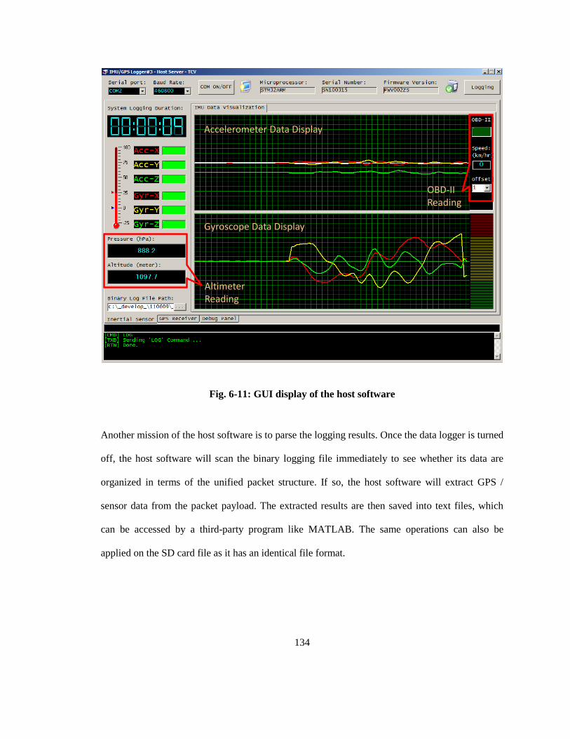
134

AltimeterReading

OBD-IIReading

Accelerometer Data Display

Gyroscope Data Display

Fig. 6-11: GUI display of the host software

Another mission of the host software is to parse the logging results. Once the data logger is turned

off, the host software will scan the binary logging file immediately to see whether its data are

organized in terms of the unified packet structure. If so, the host software will extract GPS /

sensor data from the packet payload. The extracted results are then saved into text files, which

can be accessed by a third-party program like MATLAB. The same operations can also be

applied on the SD card file as it has an identical file format.

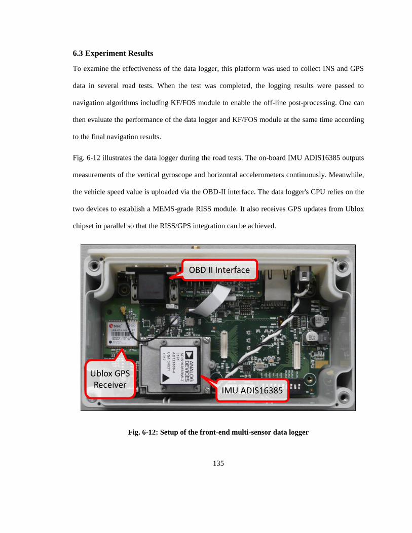
135

6.3 Experiment Results

To examine the effectiveness of the data logger, this platform was used to collect INS and GPS

data in several road tests. When the test was completed, the logging results were passed to

navigation algorithms including KF/FOS module to enable the off-line post-processing. One can

then evaluate the performance of the data logger and KF/FOS module at the same time according

to the final navigation results.

Fig. 6-12 illustrates the data logger during the road tests. The on-board IMU ADIS16385 outputs

measurements of the vertical gyroscope and horizontal accelerometers continuously. Meanwhile,

the vehicle speed value is uploaded via the OBD-II interface. The data logger's CPU relies on the

two devices to establish a MEMS-grade RISS module. It also receives GPS updates from Ublox

chipset in parallel so that the RISS/GPS integration can be achieved.

Fig. 6-12: Setup of the front-end multi-sensor data logger

136

The data logger shown in Fig. 6-12 was mounted to a testing van. The same high-end system

(NovAtel ProPack SPAN unit) used in Chapter 5 was installed beside the logger to provide a

reference solution. Several road tests were conducted using the above setup and one trajectory is

presented here to demonstrate the typical results. This trajectory is in the City of Calgary, Alberta,

Canada. In about 80 minutes, the testing van traveled over 42 km with some stops. The trajectory

mainly consists of urban streets and roads. To examine the performance of KF/FOS module, eight

artificial GPS outages are intentionally introduced. Each outage lasts for 60 seconds and all of

them cover the straight portions, turns, slopes, and stops in the trajectory. Their locations are

indicated by circles overlaid on Fig. 6-13.

Fig. 6-13: Road test trajectory in Calgary, Alberta. Circles indicate the locations of GPS

outages.

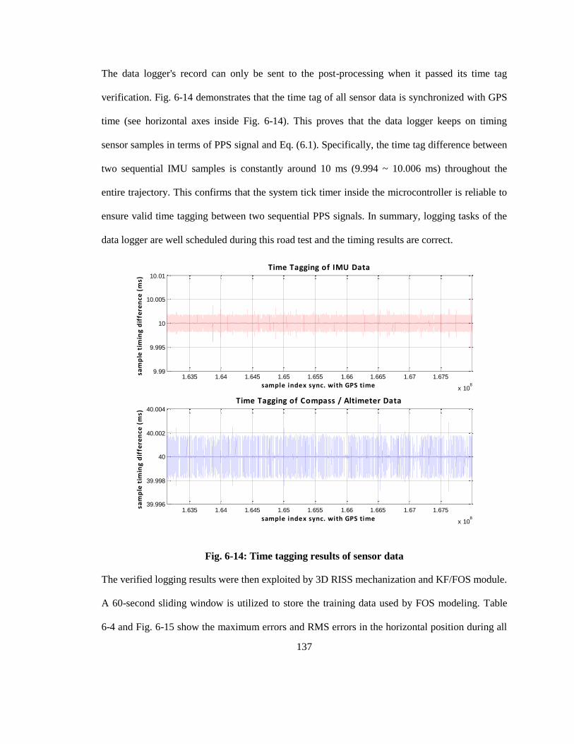
137

The data logger's record can only be sent to the post-processing when it passed its time tag

verification. Fig. 6-14 demonstrates that the time tag of all sensor data is synchronized with GPS

time (see horizontal axes inside Fig. 6-14). This proves that the data logger keeps on timing

sensor samples in terms of PPS signal and Eq. (6.1). Specifically, the time tag difference between

two sequential IMU samples is constantly around 10 ms (9.994 ~ 10.006 ms) throughout the

entire trajectory. This confirms that the system tick timer inside the microcontroller is reliable to

ensure valid time tagging between two sequential PPS signals. In summary, logging tasks of the

data logger are well scheduled during this road test and the timing results are correct.

1.635 1.64 1.645 1.65 1.655 1.66 1.665 1.67 1.675

x 108

9.99

9.995

10

10.005

10.01

sample index sync. with GPS time

sam

ple

tim

ing

dif

fere

nce

(m

s)

Time Tagging of IMU Data

1.635 1.64 1.645 1.65 1.655 1.66 1.665 1.67 1.675

x 108

39.996

39.998

40

40.002

40.004

sample index sync. with GPS time

sam

ple

tim

ing

dif

fere

nce

(m

s)

Time Tagging of Compass / Altimeter Data

Fig. 6-14: Time tagging results of sensor data

The verified logging results were then exploited by 3D RISS mechanization and KF/FOS module.

A 60-second sliding window is utilized to store the training data used by FOS modeling. Table

6-4 and Fig. 6-15 show the maximum errors and RMS errors in the horizontal position during all

138

the 60-second GPS outages for both KF/FOS and KF-only methods with respect to the NovAtel

reference. Clearly, the KF/FOS module outperformed the KF-only solution in all the GPS outages.

On average, their maximum position errors are 11.32 m and 47.19 m, respectively. This means

that KF/FOS module introduces over 70% enhancement on positioning accuracy with respect to

KF-only results. The consistency of KF/FOS performance here and in Chapter 5 reconfirms the

effectiveness of this module.


outages

GPS

outage

Avg. speed

(km / hr)

App. Dist.

(m)

KF/FOS max

Pos. Err. (m)

KF-only max

Pos. Err. (m)

KF/FOS RMS

Pos. Err. (m)

KF-only RMS

Pos. Err. (m)

1 8.2 139.7 11.73 47.79 10.29 29.41

2 41.3 699.9 13.24 32.01 10.47 21.82

3 21.7 367.8 9.90 43.77 6.58 28.14

4 70.3 1191.3 14.72 71.28 7.56 40.61

5 39.9 675.4 19.92 51.30 11.78 24.08

6 21.6 365.3 12.36 65.57 6.12 40.50

7 3.9 66.9 2.41 28.37 1.72 16.37

8 4.1 70.1 6.25 37.38 2.19 11.36

Avg. 26.4 447.0 11.32 47.19 7.09 26.54

139


outages

To throughly examine how accurate the nonlinear azimuth error model is, it is suggested to

compare the maximum azimuth errors during all the 60-second GPS outages of this trajectory for

both KF-only and KF/FOS methods. According to Fig. 6-16 and Table 6-5, the maximum

azimuth error of KF-only solution increases monotonically from 1.61◦ (in GPS outage #1) to

46.02◦ (in GPS outage #8). KF/FOS module slows down this growing process and restrains its

maximum azimuth error less than 8◦.

Fig. 6-16: Maximum azimuth errors during 60-second GPS outages

140

The ascending maximum azimuth errors of KF-only approach reveal the rapid growth of

nonlinear azimuth error and the MEMS grade gyroscope drifting. If the nonlinear error estimation

of KF/FOS is unreliable, the proposed method should suffer from the same problem. However,

since the maximum azimuth error of KF/FOS is pretty much smaller and stable, it is evident that

the FOS model is able to describe and predict the nonlinear error behaviors accurately. Taking the

model outputs as the error compensation, KF/FOS module reduces the nonlinear azimuth error

drastically and, thus, offers better positioning results.

Table 6-5: Maximum azimuth errors of KF-only and KF/FOS methods during 60-second

GPS outages

GPS outage 1 2 3 4 5 6 7 8 Avg.

KF-only max

azi. err. (deg)

1.61 4.35 5.49 7.95 14.72 24.49 41.74 46.02 18.30

KF/FOS max

azi. err. (deg)

0.91 1.91 1.62 1.15 1.41 2.47 4.56 7.51 2.69

The experiment results of this chapter prove that the front-end multi-sensor data logger is a

qualified platform to collect INS/GPS data in real time. It is also a very good test-bench to

prototype different navigation algorithms. For instance, the effectiveness of KF/FOS module is

reconfirmed on the data set offered by this logger.

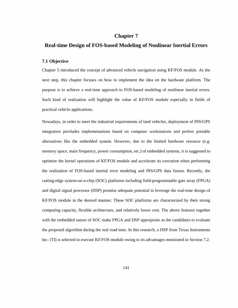
141

Chapter 7

Real-time Design of FOS-based Modeling of Nonlinear Inertial Errors

7.1 Objective

Chapter 5 introduced the concept of advanced vehicle navigation using KF/FOS module. As the

next step, this chapter focuses on how to implement the idea on the hardware platform. The

purpose is to achieve a real-time approach to FOS-based modeling of nonlinear inertial errors.

Such kind of realization will highlight the value of KF/FOS module especially in fields of

practical vehicle applications.

Nowadays, in order to meet the industrial requirements of land vehicles, deployment of INS/GPS

integration precludes implementations based on computer workstations and prefers portable

alternatives like the embedded system. However, due to the limited hardware resource (e.g.

memory space, main frequency, power consumption, etc.) of embedded systems, it is suggested to

optimize the kernel operations of KF/FOS module and accelerate its execution when performing

the realization of FOS-based inertial error modeling and INS/GPS data fusion. Recently, the

cutting-edge system-on-a-chip (SOC) platforms including field-programmable gate array (FPGA)

and digital signal processor (DSP) promise adequate potential to leverage the real-time design of

KF/FOS module in the desired manner. These SOC platforms are characterized by their strong

computing capacity, flexible architecture, and relatively lower cost. The above features together

with the embedded nature of SOC make FPGA and DSP appropriate as the candidates to evaluate

the proposed algorithm during the real road tests. In this research, a DSP from Texas Instruments

Inc. (TI) is selected to execute KF/FOS module owing to its advantages mentioned in Section 7.2.

142

The major objective of this chapter is to develop a prototype TI DSP-based navigation and

guidance system for land vehicles. It will be a fully featured, real-time, in-vehicle, low cost

embedded system that contains the GPS receiver and INS sensors.

Detailed objectives are:

(1) Research and development on TI DSP hardware platform to implement a standalone

embedded system that combines a GPS receiver and inertial sensors together using

flexible communication and peripheral interfaces.

(2) Research and development on TI DSP hardware platform to apply a hybrid INS/GPS

real-time data fusion module that relies on FOS-based nonlinear modeling of inertial

errors and Kalman filtering of linear inertial errors.

(3) Optimizing the embedded software package of FOS kernel and KF operations in order to

make them efficient, reliable, scalable, and portable for DSP targets.

(4) To enable the online vehicle navigation based on objective 1 and 2 throughout road tests.

Rather than post-processing logged INS/GPS data after road tests as shown when

evaluate the concept of KF/FOS module in Chapter 5, the work scheme here should

warrantee the latency between the inputs of front end data collection and the outputs of

corresponding navigation results never exceeds one second. This requirement is

fundamental to validate the real-time ability of the proposed technique.

(5) To develop professional human interfaces on DSP targets and PC hosts to analysis and

monitor the calculation of KF/FOS module and INS/GPS integration.

143

7.2 DSP-based Hardware Implementation of KF/FOS Module

7.2.1 Platform Selection

Section 7.1 recommended FPGA and DSP as the candidate platforms to run KF/FOS module. In

fact, at present, most of the digital signal processing applications is commonly implemented on

these two types of programmable devices. DSP is a specialized microprocessor equipped by high

efficient computing unit (e.g. hardware multiplier) and data path (e.g. Harvard bus system). These

built-in resources make DSP very suitable to extremely complex tasks involving with intensive

mathematical operations and conditional processing. In contrast, FPGA, as outlined by its name,

contains uncommitted array of logic gates with a huge amount. Developers need to program it by

connecting the gates together and then building up registers, adders, multipliers, and so forth for

their specific applications. The primary distinction in the architecture results in totally different

approaches to signal processing: FPGA depends on block diagrams or more flexible hardware

description languages like Verilog and VHDL to organize its highly configurable hardware;

whereas DSP is running instructions generated from C programming language or assembly code

to make full use of its powerful computing resource offered by a fixed hardware structure. Each

one of them fits different areas due to its own characteristic. Corresponding comparison can be

found in reference [84] as well. In this study, the selection between DSP and FPGA is subject to

the specific requirements of KF/FOS module and vehicle navigation. The criteria are ranked as

follows:

1. Floating point support

In digital computing, a fixed point number representation is a real data type of a number that has

fixed numbers before and after the radix point. Because of the fixed window of representation,

fixed point number has limits to represent very large or very small numbers. Also, fixed point

144

calculation is prone to a loss of precision when inevitable rounding is needed to comply with the

restriction of word length. A more accurate data type is the floating point, which represents real

numbers in a wider range with the precision appropriate to the scale of the numbers. Using this

manner, the numbers are in general represented by a fixed number of significant digits and scaled

by an exponent. A typical real number R can be presented in floating point by Eq.(7.1), where s is

the value of significand including the implied radix point and leading digit; b is the base; e is the

exponent; a is the exponent bias ensuring the equality of positive and negative exponent ranges.

e aR s b (7.1)

Fig. 7-1 illustrates the 32-bit structure of IEEE single precision floating point number. The upper

limit and lower limit of 8-bit exponent are 127 and -126 (128 and -127 are preserved for special

numbers [85]), respectively, after taking the bias value 127 into account. Given the 23-bit fraction

and the base value as 2, the dynamic range of a normalized single precision floating point number

is [± 2-126

, ± (2-2-23

)×2127

] or approximately [±10-38

, ±1038

]. In contrast, a 32-bit fixed point

number with 16-bit decimal portion and one sign bit can only cover a range of [±2-16

, ±215

] or

approximately [±10-5

, ±105]. Clearly, possible rounding errors at level of 10

-5 can propagate and

grow over time in the integral of RISS mechanization. Their undesired error contribution may

lead to quantization noise and nonlinear distortions that are even comparable to inertial sensor

errors. Meanwhile, overflow errors jeopardize the reliability of calculation when the upper limit

of operands is only up to 105. Owing to its mechanism, floating point calculation does not suffer

from the above limitations and shows advantages on computing accuracy.

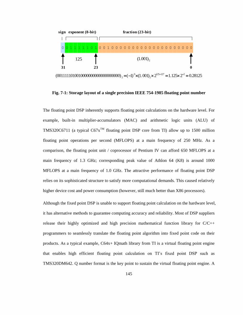
145

0 0 1 1 1 1 1 0 1 0 0 1 0 0 0 0 0 0 0 0 0 0 0 0 0 0 0 0 0 0 0 0

02331

fraction (23-bit)exponent (8-bit)sign

0 125 127 2

2 2(00111110100100000000000000000000) ( 1) (1.001) 1.2 2125 0.28125

2(1.001)125

Fig. 7-1: Storage layout of a single precision IEEE 754-1985 floating point number

The floating point DSP inherently supports floating point calculations on the hardware level. For

example, built-in multiplier-accumulators (MAC) and arithmetic logic units (ALU) of

TMS320C6711 (a typical C67xTM

floating point DSP core from TI) allow up to 1500 million

floating point operations per second (MFLOPS) at a main frequency of 250 MHz. As a

comparison, the floating point unit / coprocessor of Pentium IV can afford 650 MFLOPS at a

main frequency of 1.3 GHz; corresponding peak value of Athlon 64 (K8) is around 1000

MFLOPS at a main frequency of 1.0 GHz. The attractive performance of floating point DSP

relies on its sophisticated structure to satisfy more computational demands. This caused relatively

higher device cost and power consumption (however, still much better than X86 processors).

Although the fixed point DSP is unable to support floating point calculation on the hardware level,

it has alternative methods to guarantee computing accuracy and reliability. Most of DSP suppliers

release their highly optimized and high precision mathematical function library for C/C++

programmers to seamlessly translate the floating point algorithm into fixed point code on their

products. As a typical example, C64x+ IQmath library from TI is a virtual floating point engine

that enables high efficient floating point calculation on TI’s fixed point DSP such as

TMS320DM642. Q number format is the key point to sustain the virtual floating point engine. A

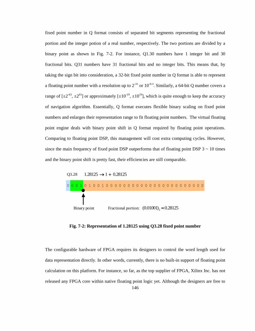
146

fixed point number in Q format consists of separated bit segments representing the fractional

portion and the integer potion of a real number, respectively. The two portions are divided by a

binary point as shown in Fig. 7-2. For instance, Q1.30 numbers have 1 integer bit and 30

fractional bits. Q31 numbers have 31 fractional bits and no integer bits. This means that, by

taking the sign bit into consideration, a 32-bit fixed point number in Q format is able to represent

a floating point number with a resolution up to 2-31

or 10-9.3

. Similarly, a 64-bit Q number covers a

range of [±2-63

, ±263

] or approximately [±10-19

, ±1019

], which is quite enough to keep the accuracy

of navigation algorithm. Essentially, Q format executes flexible binary scaling on fixed point

numbers and enlarges their representation range to fit floating point numbers. The virtual floating

point engine deals with binary point shift in Q format required by floating point operations.

Comparing to floating point DSP, this management will cost extra computing cycles. However,

since the main frequency of fixed point DSP outperforms that of floating point DSP 3 ~ 10 times

and the binary point shift is pretty fast, their efficiencies are still comparable.

0 0 0 1 0 1 0 0 1 0 0 0 0 0 0 0 0 0 0 0 0 0 0 0 0 0 0 0 0 0 0 0

Q3.28

Binary point Fractional portion: 2(0.01001) 0.28125

1.28125 1 0.28125

Fig. 7-2: Representation of 1.28125 using Q3.28 fixed point number

The configurable hardware of FPGA requires its designers to control the word length used for

data representation directly. In other words, currently, there is no built-in support of floating point

calculation on this platform. For instance, so far, as the top supplier of FPGA, Xilinx Inc. has not

released any FPGA core within native floating point logic yet. Although the designers are free to

147

develop their own, the task will be time-consuming and the quality of their product may not catch

up with off-the-shelf industrial grade solutions. On the other hand, all the built-in or virtual

floating point operations on DSP are transparent to its developers. This allows them to

concentrate on their rapid development for specific applications without any worry about the

availability and efficiency of floating point calculation. As a result, the prototype verification of

navigation algorithms can be more easily achieved on DSP.

Recently, soft processor cores like Micro-Blaze from Xilinx and NIOS II from Altera are applied

on FPGA to enable more complicated algorithm design. Owing to the configuration of these

intellectual property (IP) cores, FPGA is able to behave in the same manner as a general purpose

RISC processor. It can then benefit from higher level numerical packages to breakthrough its

floating point limitations at certain levels. However, comparing to high efficient floating point

DSP and specifically optimized virtual floating point engine, these alternatives are still in lack of

dedicated double precision floating point units. Thus, at present, DSP still shows apparent

advantages over FPGA on floating point support.

2. Parallel computing

Hardware level parallelization is one of the most distinguished advantages of FPGA. Modern

FPGA contains huge amount of logic elements (also known as logic cells). These units are

fabricated in standalone structures that usually combine multi-input look-up-table (LUT), flip-

flops, latches, and multiplexers together in flexible styles (shown in Fig. 7-3). As a primary

component, the logic element alone can be programmed as simple as a slice of memory unit or a

logic gate. Alternatively, they can also be interconnected in group to build a reconfigurable

hierarchy also known as logic array or logic block. After being routed in a programmable scheme,

logic blocks can be wired up together in large scales to perform complex combinational and

148

sequential logic for specific requirements. Such sorts of configuration can be collected as IP cores

that implement high speed FIFO, SRAM, DSP MAC unit, or even multi-core soft

microprocessors on FPGA. Thanks to this mechanism, FPGA can be customized to have plenty

of different sub-systems and powerful arithmetic modules working in parallel. This explains why

high-end FPGA provides more computing resources than its DSP competitor.

DSP supports parallel operations as well. As an instruction-set based processor, TI C6000 DSP

has an 8-level pipeline and 8 highly independent functional units that work together to carry on

instruction fetching, decoding, executing, and memory access simultaneously. More advanced

concepts like the very-long-instruction-word and superscalar allow it to access and execute

multiple instructions entirely in parallel. These features are of specific interest for intensive

iterations such as Gram-Schmidt process used by FOS.

Fig. 7-3: A 4-input logic element (LE) block diagram (Altera’s Stratix FPGA family) [86]

Comparing to FPGA, the parallelism of DSP is at instruction level and bounded to single

processor. Therefore, the cooperative parallel between processing units on FPGA is more

appropriate to deal with massive concurrent data in greater bandwidth such as the measurements

149

of medical imaging and synthetic aperture radars. Actually, the civilian vehicle navigation

including RISS mechanization and KF/FOS module can be categorized as a sequential task. Also,

its GPS updating rate and IMU sampling rate are commonly at 1 Hz and lower than 1000 samples

per second, respectively. Therefore, the instruction level parallelism is still adequate to maintain

the real-time performance. In general, FPGA offers more powerful computing resource and

parallel operations in larger scale than DSP but also commits higher design complexity to

administrate its parallelization.

3. Efficiency in algorithm design

The algorithm design on DSP is faster and more productive. Fig. 7-4 illustrates the most common

path of software development on DSP. In the designing stage, developers can benefit from the

flexibility of C language program to rapidly implement complicated conditional operations,

branching decisions, iterations, and the other logic that intensively exist in the algorithm

prototype. Then, the optimized C/C++ compiler converts the source files to assembly code so that

DSP simulators can use them to profile the algorithm design. Owing to this feature, developer can

refine their C program or even write linear assembly that corresponds to computing hot spots.

During the procedure, the prototyping can be drastically accelerated by reusing various macro and

run-time libraries (e.g. IQmath) either from DSP vendors or third parties. In the verification stage,

the assembler works together with the linker to generate object files and, eventually, executable

code. Debugging tools like the emulators can then download the executable code to target DSP

and allow the interactive debugging afterwards. Overall, the DSP tool-chain is seamlessly

integrated to cover the entire software development cycle so that developers can get rid of

technical details and concentrate on algorithm prototyping.

150

Fig. 7-4: TI TMS320C6000 DSP software development flow [87]

Algorithm design on FPGA requires greater efforts. Their schematic or block diagram inputs have

limitations to implement complicated logic quickly. Hardware languages like Verilog and VHDL

cannot catch up with C/C++ program to describe the algorithm concisely neither. As a result,

developers have to spend much more time on technical details such as the construction of ALU

and buffer structures rather than the more important algorithm prototyping. Moreover, there exist

extra tasks for developers to implement the test vectors by themselves. As the only way to

thoroughly examine the FPGA designs, this method yields less productivity than the interactive

151

debugging on DSP. Although soft processor core is able to relieve the workload, designers still

have to take care of the development environment and accept the loss of performance. In

summary, DSP is more practical than FPGA to maintain the efficiency of algorithm design.

4. Power consumption and device cost

Power requirements are typically much higher for FPGA than other hardware platforms [88].

Low-end and common FPGAs do not have dedicated power management units by default. The

high-end products support this feature with much higher price. As a result, the designer has to

give extra efforts to figure out the trade-off between the system expense and power consumption

when using FPGA in cost-sensitive vehicle navigation.

In contrast, power management units have become the fundamental component inside modern

embedded microprocessors including DSP. They can either work alone in background to save

power by switching CPU working mode between the idle stage and busy stage or cooperate with

the operating system to monitor the entire power status. The flexible power management

facilitates the application of DSP in portable and power restrained fields such as the vehicle.

At present, DSP keep advantages over FPGA on the device cost. This is more prominent for their

high-end products. As a comparison, the average price of C6000 DSP from TI is lower than $50,

whereas any member of Xilinx Virtex-IV family (middle density FPGA) can cost more than $300

in retail. Obvious, DSP is better to satisfy the low cost requirement of RISS/GPS integration.

After thoroughly comparing the two platforms in the floating point support, parallel computing,

algorithm design efficiency, power consumption and device cost, DSP is selected as the

workbench to implement real-time RISS/GPS integration and KF/FOS module. Other candidates

were not selected due to their own shortcomings. E.g. ASIC asks for a very high price. ARM

processors keep low device cost, but are unable to offer the same computing capacity as DSP yet.

152

7.2.2 System Architecture

Discussions in Chapter 4 and Chapter 5 reveal the recursive nature of KF/FOS module. Hence,

this approach is very suitable to be applied on a digital computer. In this research,

TMS320DM642, a fixed point general purpose DSP from TI, is utilized as the embedded

computing platform to carry out the real-time algorithm prototyping. To support the collection

and buffer of INS/GPS data, external peripherals like the UART and DRAM are required as well.

They exchange information with DSP either through the common bus or via more efficient

external memory interfaces. All the devices are laid out on a print circuit board also known as

DM642 evaluation module (EVM). Table 7-1 presented the basic information of DM642 and its

EVM.

Table 7-1: Relevant features of TMS320DM642 DSP and its EVM

Specification overview of TMS320DM642 DSP core

Peak multiply operations per second 5760 million

Main frequency 720 MHz

On-chip memory space 32 KB Level-1 cache, 256 KB Level-2 cache

Specification overview of DM642 EVM

Main processor Fixed point TMS320DM642 DSP

On-board memory space 32 MB DRAM, 4 MB Flash

Peripheral interface Dual UART

Regarding the actual system organization, another sub-module within at least 4 UART ports is

needed to assist the front-end data collection. It works like the data logger in Chapter Five to

receive the data stream of GPS signals, rotation rates on the vertical direction, forward and

transversal accelerations, as well as the vehicle forward speed from the GPS receiver, the MEMS-

153

based IMU, and the odometer, respectively. Once the above data are well synchronized and ready

to use, the sub-model uploads them to DM642 EVM immediately via the RS232 protocol on the

remaining UART. From the point of view of DSP, when a new package of the above data is

available, it executes the calculation of RISS mechanization and RISS/GPS data fusion using

KF/FOS module sequentially for one time. Due to its strong computing capacity, DSP ensures

that all these calculations can be completed before the arrival of the next data package sent by the

logger. Consequently, the whole system is able to sample and process GPS/INS data in the

continuous mode such that the DSP core can achieve real-time RISS/GPS integration and offer

online navigation results as outlined in subsection 7.1. Optionally, the DSP computing results can

be uploaded to a workstation through the remaining UART on DM642 EVM to enable

monitoring. Fig. 7-5 depicts the block diagram described above.

Fig. 7-5: DSP-based 3D RISS/GPS integration

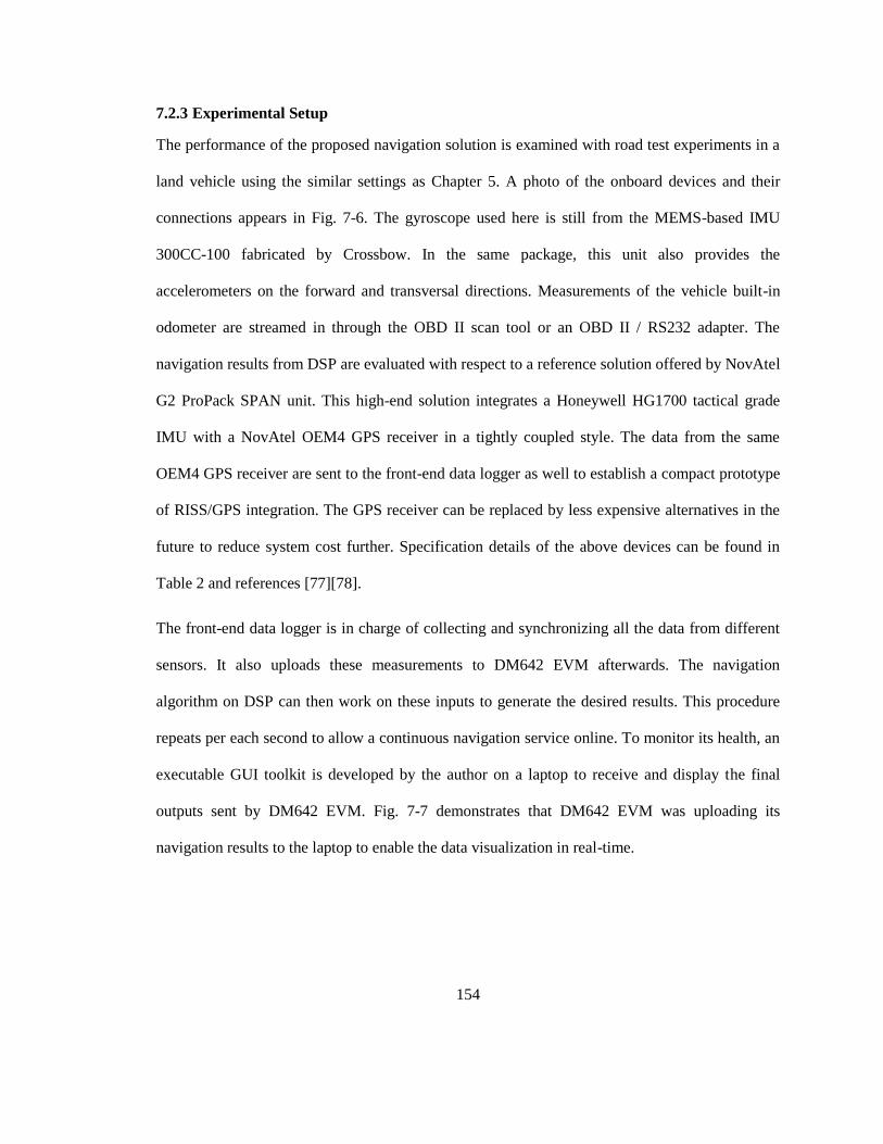
154

7.2.3 Experimental Setup

The performance of the proposed navigation solution is examined with road test experiments in a

land vehicle using the similar settings as Chapter 5. A photo of the onboard devices and their

connections appears in Fig. 7-6. The gyroscope used here is still from the MEMS-based IMU

300CC-100 fabricated by Crossbow. In the same package, this unit also provides the

accelerometers on the forward and transversal directions. Measurements of the vehicle built-in

odometer are streamed in through the OBD II scan tool or an OBD II / RS232 adapter. The

navigation results from DSP are evaluated with respect to a reference solution offered by NovAtel

G2 ProPack SPAN unit. This high-end solution integrates a Honeywell HG1700 tactical grade

IMU with a NovAtel OEM4 GPS receiver in a tightly coupled style. The data from the same

OEM4 GPS receiver are sent to the front-end data logger as well to establish a compact prototype

of RISS/GPS integration. The GPS receiver can be replaced by less expensive alternatives in the

future to reduce system cost further. Specification details of the above devices can be found in

Table 2 and references [77][78].

The front-end data logger is in charge of collecting and synchronizing all the data from different

sensors. It also uploads these measurements to DM642 EVM afterwards. The navigation

algorithm on DSP can then work on these inputs to generate the desired results. This procedure

repeats per each second to allow a continuous navigation service online. To monitor its health, an

executable GUI toolkit is developed by the author on a laptop to receive and display the final

outputs sent by DM642 EVM. Fig. 7-7 demonstrates that DM642 EVM was uploading its

navigation results to the laptop to enable the data visualization in real-time.

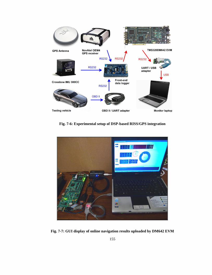
155

Fig. 7-6: Experimental setup of DSP-based RISS/GPS integration

Fig. 7-7: GUI display of online navigation results uploaded by DM642 EVM

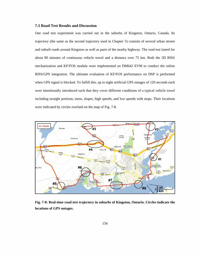
156

7.3 Road Test Results and Discussion

One road test experiment was carried out in the suburbs of Kingston, Ontario, Canada. Its

trajectory (the same as the second trajectory used in Chapter 5) consists of several urban streets

and suburb roads around Kingston as well as parts of the nearby highway. The road test lasted for

about 80 minutes of continuous vehicle travel and a distance over 75 km. Both the 3D RISS

mechanization and KF/FOS module were implemented on DM642 EVM to conduct the online

RISS/GPS integration. The ultimate evaluation of KF/FOS performance on DSP is performed

when GPS signal is blocked. To fulfill this, up to eight artificial GPS outages of 120 seconds each

were intentionally introduced such that they cover different conditions of a typical vehicle travel

including straight portions, turns, slopes, high speeds, and low speeds with stops. Their locations

were indicated by circles overlaid on the map of Fig. 7-8.

Fig. 7-8: Real-time road test trajectory in suburbs of Kingston, Ontario. Circles indicate the

locations of GPS outages.

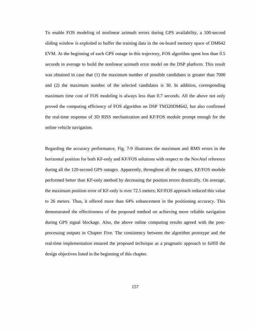
157

To enable FOS modeling of nonlinear azimuth errors during GPS availability, a 100-second

sliding window is exploited to buffer the training data in the on-board memory space of DM642

EVM. At the beginning of each GPS outage in this trajectory, FOS algorithm spent less than 0.5

seconds in average to build the nonlinear azimuth error model on the DSP platform. This result

was obtained in case that (1) the maximum number of possible candidates is greater than 7000

and (2) the maximum number of the selected candidates is 30. In addition, corresponding

maximum time cost of FOS modeling is always less than 0.7 seconds. All the above not only

proved the computing efficiency of FOS algorithm on DSP TM320DM642, but also confirmed

the real-time response of 3D RISS mechanization and KF/FOS module prompt enough for the

online vehicle navigation.

Regarding the accuracy performance, Fig. 7-9 illustrates the maximum and RMS errors in the

horizontal position for both KF-only and KF/FOS solutions with respect to the NovAtel reference

during all the 120-second GPS outages. Apparently, throughout all the outages, KF/FOS module

performed better than KF-only method by decreasing the position errors drastically. On average,

the maximum position error of KF-only is over 72.5 meters; KF/FOS approach reduced this value

to 26 meters. Thus, it offered more than 64% enhancement in the positioning accuracy. This

demonstrated the effectiveness of the proposed method on achieving more reliable navigation

during GPS signal blockage. Also, the above online computing results agreed with the post-

processing outputs in Chapter Five. The consistency between the algorithm prototype and the

real-time implementation ensured the proposed technique as a pragmatic approach to fulfill the

design objectives listed in the beginning of this chapter.

158

Fig. 7-9: (A) Maximum position error and (B) RMS position error during GPS outages

In order to reveal how accurate the FOS model is and why its prediction can improve the overall

navigation performance, the RMS azimuth error during GPS outages for both KF-only and

KF/FOS methods are presented in Fig. 7-10. While the trajectory proceeds, KF-only azimuth

error is increasing significantly and, thus, evolves into the major error source. This is due to the

fact that, as an optimal linear estimator, KF alone is unable to suppress the growth of nonlinear

azimuth error caused by the unstable scale factor and bias drift in the MEMS-based inertial

sensors. Other possible challenges such as the aftermath of KF mis-modeling lead to even worse

deterioration. These error effects, in turn, result in rapid positioning error growth. Clearly, Fig.

7-10 demonstrated the ascending trend of KF-only azimuth error over time. In contrast, the

azimuth errors of KF/FOS module keep relatively stable throughout all the GPS outages and are

always much less than those of KF-only solution. The smaller heading angle error surely causes

better navigation performance. The results prove the accurate modeling and compensation of

nonlinear azimuth errors offered by KF/FOS module in the real-time scenario.

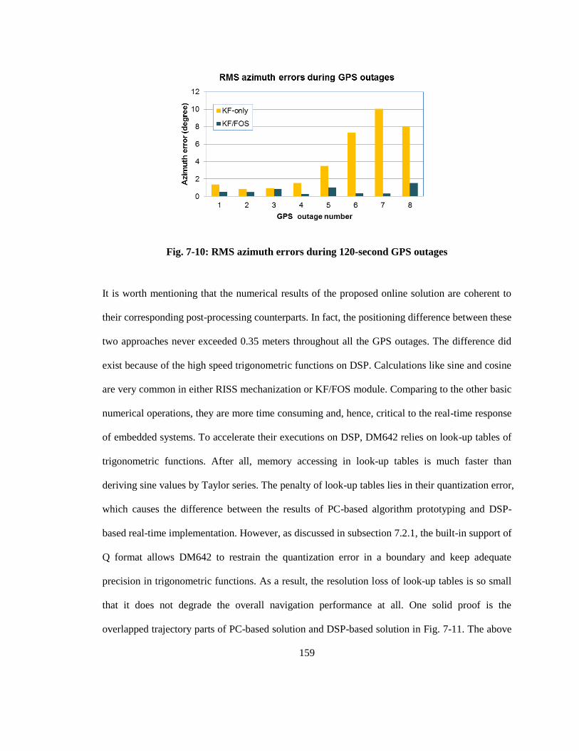
159

Fig. 7-10: RMS azimuth errors during 120-second GPS outages

It is worth mentioning that the numerical results of the proposed online solution are coherent to

their corresponding post-processing counterparts. In fact, the positioning difference between these

two approaches never exceeded 0.35 meters throughout all the GPS outages. The difference did

exist because of the high speed trigonometric functions on DSP. Calculations like sine and cosine

are very common in either RISS mechanization or KF/FOS module. Comparing to the other basic

numerical operations, they are more time consuming and, hence, critical to the real-time response

of embedded systems. To accelerate their executions on DSP, DM642 relies on look-up tables of

trigonometric functions. After all, memory accessing in look-up tables is much faster than

deriving sine values by Taylor series. The penalty of look-up tables lies in their quantization error,

which causes the difference between the results of PC-based algorithm prototyping and DSP-

based real-time implementation. However, as discussed in subsection 7.2.1, the built-in support of

Q format allows DM642 to restrain the quantization error in a boundary and keep adequate

precision in trigonometric functions. As a result, the resolution loss of look-up tables is so small

that it does not degrade the overall navigation performance at all. One solid proof is the

overlapped trajectory parts of PC-based solution and DSP-based solution in Fig. 7-11. The above

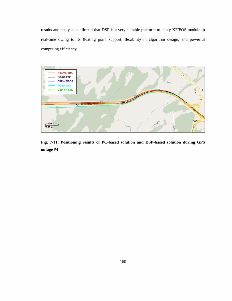
160

results and analysis confirmed that DSP is a very suitable platform to apply KF/FOS module in

real-time owing to its floating point support, flexibility in algorithm design, and powerful

computing efficiency.

Fig. 7-11: Positioning results of PC-based solution and DSP-based solution during GPS

outage #4

161

Chapter 8

Conclusions and Future Work

8.1 Conclusions

This thesis aimed at introducing new nonlinear techniques to enhance the performance of low

cost positioning systems for land vehicles. It firstly reviewed present navigation approaches and

then decided on INS/GPS integration as its main focus. To enable low cost navigation, this thesis

suggested integrating GPS with a low cost INS built by fewer MEMS grade sensors. This setup

was challenged by intensive nonlinear system errors and stochastic sensor noise, which cannot be

mitigated by conventional linear filters. After analyzing the corresponding error characteristics,

this research suggested to utilize Fast Orthogonal Search, a numerical nonlinear system

identification technique, to model and handle the nonlinear errors of low cost MEMS-grade INS.

An augmented KF/FOS module was proposed to suppress both linear and nonlinear error effects.

Its effectiveness in enhancing the navigation accuracy is verified during GPS outages of different

road test trajectories. A data logger acquiring and synchronizing the sensor measurements in real-

time was developed as part of this thesis. Moreover, a hardware implementation of KF/FOS

module was applied on a digital signal processor to evaluate the real-time capability of the

proposed solution. Experimental results demonstrated the performance of the embedded platform

for online vehicle navigation in the real life.

Chapter 2 reviewed various navigation approaches popular at present. Among them, both GPS

and INS are widely utilized in vehicle navigation. Although GPS alone is able to guarantee long

term accuracy, in certain environments, it suffers from possible signal interference, reflection, and

blockage that cause its accuracy deterioration or even service outages. In contrast, INS keeps on

continuous navigation at much higher data rates. As a self-contained system, it is immune to

162

external interference. Nevertheless, its accuracy is threatened by the unbounded growth of its own

sensor errors. The complementary features of GPS and INS motivate their integration that offers

better performance than the INS or GPS standalone solution. For low cost applications, MEMS

grade INS is preferred due to its low product price, low power consumption, small size, and light

weight. To reduce the system cost further, the INS used in this study comprised only one MEMS-

grade single axis gyroscope and the vehicle built-in odometer for 2D cases. This reduced inertial

sensor system can be optionally augmented by two MEMS grade accelerometers to accommodate

3D positioning requirements.

The data fusion of INS and GPS is commonly achieved by Kalman filter. KF-based INS/GPS

integration provides adequate performance in case of high-end inertial sensors. When using low

cost MEMS grade INS, its accuracy is severely influenced by the rapid growth of nonlinear INS

errors, which are caused by the non-stationary stochastic MEMS sensor errors. As an optimal

linear estimator, KF is unable to compensate for these higher order errors. To solve this problem,

FOS algorithm is proposed to deal with the signal nonlinearity. As introduced in Chapter 4, FOS

systematically examines all the possible candidates built by arbitrary higher order terms or cross-

products of the system inputs. It selects those candidates that maximize reduction of the model-fit

mean-square-error in sequence. The selected candidates can then be used to build the nonlinear

model that approaches to the original system. This procedure repeats recursively until certain stop

criteria have been met. Eventually, the FOS model can be accurate enough to describe the

nonlinear system being considered. When applied in INS/GPS integration, FOS algorithm is

suggested to cascade with KF to construct a KF/FOS module, which reduces both linear and

nonlinear INS errors. During GPS availability, the use of FOS algorithm guarantees the accurate,

yet still efficient modeling of non-stationary stochastic sensor errors (i.e. the gyro drift in this

study) and nonlinear azimuth errors. When GPS outages occur, the latest pre-built model predicts

163

and compensates the above errors. Consequently, the proposed method is able to overcome the

limitations of KF-only solution and improve the positioning accuracy drastically.

The effectiveness of KF/FOS module was evaluated during GPS outages of different trajectories.

Its test-bench is a platform that integrates GPS with a MEMS grade RISS in a loosely coupled

manner for both 2D and 3D cases. The experiment results in Chapter 5 illustrated the fact that, in

60-second and 120-second GPS outages, KF/FOS module introduces over 60% enhancement of

positioning accuracy on average with respect to the KF-only solution. It takes less than 0.1

seconds on X86 PC (Intel Pentium-4 at 2.8 GHz / 2GB DDR2) for FOS algorithm to build the

model used in the above tests when a 100-second sliding window is used to collect the training

data.

To achieve the real-time vehicle navigation, the first step was to collect online INS/GPS data

needed by INS mechanization and KF/FOS module. A front-end data logger was designed to

satisfy this requirement. It synchronized the data stream from both INS and GPS by time tagging

their samples. The timing results together with the raw multi-sensor data were then wrapped into

packets. Since all these packets comply with a unified format, they can either be passed to online

navigation algorithm directly or stored for post-processing. Essentially, the logger works as a hub

to assemble multi-sensor measurements and upload them via a standard interface. This allows the

host machine to focus on INS/GPS data fusion rather than caring about data collection details.

KF/FOS module was then transplanted on a DSP-based hardware platform (TMS320DM642

EVM at 720 MHz) to perform the online vehicle navigation. Keeping the same condition

presented in Chapter 5, the embedded hardware design takes about 0.5 seconds on average and

0.7 seconds at most to build the FOS model. This ensures that the design is always able to output

navigation results at 1Hz throughout the road test trajectory. Also, the positioning accuracy of the

164

embedded hardware design is consistent to that of the theoretical prototype developed on PC.

Experiment results in Chapter 7 proved that the proposed technique has advantages on both

navigation performance and real-time response for vehicle applications in the real life.

8.2 Recommendations of Future Work

As an innovative navigation technique, KF/FOS module shows great advantages in this study on

improving the performance of low cost positioning systems. To further enhance this technique,

several future works are suggested in the followings.

1. Cascade of FOS and the other nonlinear techniques

KF/FOS module is open to be cascaded by other sophisticated nonlinear techniques. For instance,

particle filtering (PF), a nonlinear estimator, is suggested as replacement to KF for the

augmentation with FOS. PF shall benefit from the accurate nonlinear model developed by FOS to

preserve the quality of its prediction. The nonlinear INS error model built by FOS is very suitable

to satisfy this requirement. The combination of the FOS and PF should be able to refine the

compensation of nonlinear INS errors and, thus, provide superior navigation performance.

2. Increasing the data rate of KF/FOS module

KF/FOS module outputs positioning results at 1 Hz in this study. This data rate is adequate for

ordinary real-time vehicle applications. However, if positioning is not the ultimate purpose but a

step in the feedback loop of a guidance system, it will need a higher data rate to catch up with the

pace of guidance control. For instance, to ensure collision avoidance of autonomous vehicle or

robots, the braking time of their guidance systems is always less than 0.6 seconds. During this

period, the guidance system may not receive any navigation updates if KF/FOS module keeps 1-

Hz data rate. The more advanced anti-lock braking system (ABS) queries positioning results even

more frequently (e.g. 10 – 100 Hz) to adjust its mechanical control and avoid skidding. To

165

accommodate the above scenarios, KF/FOS module can be customized in the future to allow

more prompt response. One suggestion is to reduce the training window size and the maximum

amount of the selected candidates. Such sort of options will accelerate FOS running but needs to

be controlled in order not to degrade the modeling accuracy.

3. Applying KF/FOS module in tightly coupled INS/GPS integration

As mentioned in Chapter 2 and Chapter 5, the effectiveness of KF/FOS module is only verified in

case of the open-loop loosely coupled INS/GPS integration. Future studies are still required to

evaluate its performance in the tightly coupled approaches. To implement this idea, the Kalman

filter inside KF/FOS module will be more complicated to deal with raw GPS signals. In return,

FOS algorithm is able to keep on correcting its model even during certain GPS outages. This is

possible as the tightly coupled solution offers GPS updates even if the number of visible GPS

satellites is fewer than four. Moreover, the existence of limited GPS aiding provides another way

to monitor the quality of FOS model prediction. It has great significance to detect the possible

divergence and over-fitting of the FOS model.

4. Optimization of the real-time design on the hardware

The data logger presented in Chapter 6 has an open architecture to acquire extra sensor readings.

In fact, it has already been equipped by the on-board digital compass and altimeter. Future

enhancement can take their measurements into consideration to enlarge the scale of multi-sensor

integration. For instance, the extra sensor readings provide redundant reference to correct INS

error especially during GPS outages. Meanwhile, software profiling and optimization of KF/FOS

module can be applied on the DSP platform presented in Chapter 7. Any further improvements on

the computing efficiency will not only speed up the real-time response of KF/FOS module, but

166

also make the proposed method applicable to fulfill positioning requirements of the more

challenging guidance systems.

167

References

[1] J. Farrell, The Global Positioning System and Inertial Navigation, McGraw-Hill, New

York, 1998.

[2] I. Skog and P. Handel, “In-Car Positioning and Navigation – A Survey”, IEEE

Transactions on Intelligent Transportation Systems 10 (1), 4 – 21, March, 2009

[3] M.S. Grewal, L.R. Weill, and A.P. Andrews, Global Positioning System, Inertial

Navigation and Integration, Wiley, New York, 2001.

[4] A. Lawrence, Modern Inertial Technology, Springer Verlag, New York, 1998.

[5] D.H. Titterton and J.L. Weston, Strap-Down Inertial Navigation Technology, Peregrinus,

London, 1997.

[6] K.P. Schwarz and M. Wei, “A framework for modeling kinematic measurements in

gravity field applications”, Bulleting Geodesique 64 (4), 331 – 346, 1990.

[7] R.G. Brown and P.Y.C. Hwang, Introduction to Random Signal and Applied Kalman

Filtering: With MATLAB Exercises and Solutions, 3rd

Ed., Wiley, New York, 1997.

[8] S. Nassar, Improving the Inertial Navigation System (INS) Error Model for INS and

INS/DGPS Applications, Dissertation, University of Calgary, Alberta, Canada, 2003.

[9] A.D. King, “Inertial Navigation – Forty Years of Evolution”, GEC Review 13 (3), 140 –

149, 1998.

[10] A. Noureldin, T.B. Karamat, M.D. Eberts, and A. El-Shafie, “Performance enhancement

of MEMS based INS/GPS integration for low cost navigation applications”, IEEE

Transactions on Vehicular Technology 58 (3), 1077 – 1096, 2009.

[11] J. Borenstein, H. Everett, L. Feng, and D. Wehe, “Mobile robot positioning: Sensors and

technologies”, Journal of Robotics Systems 14 (4), 231 – 249, 1997.

[12] O.J. Woodman, “An introduction to inertial navigation”, technical report 696, Cambridge

UK, August, 2007.

[13] A.B. Chatfield, “Fundamentals of High Accuracy Inertial Navigation”, progress in

astronautics and aeronautics 174, American Institute of Aeronautics and Astronautics Inc.,

1997.

[14] C.S. Draper, “Origins of inertial navigatioin”, Journal of Guidance and Control 4 (5), 449

– 463, 1981.

[15] N. Barbour and G. Schmidt, “Inertial Sensor Technology Trends”, IEEE Sensors Journal

1 (4), 332 – 339, 2001.

168

[16] R. Torrance, “MEMS-based inertial sensor is not your grandfather’s gyroscope”,

Electronics Design, Strategy, and News, December, 2008.

[17] K. Maenaka, “Current MEMS Technology and MEMS Sensors Focusing on Inertial

Sensors”, Solid-state and Integrated Circuit Technology, ICSICT 2008, 9th International

Conference, 2371 – 2374, October, 2008.

[18] B. Jonathan, “An Overview of MEMS Inertial Sensing Technology”, Corning-

IntelliSense Corp., Wilmington, MA, 2003.

[19] J.L., Weston and D.H. Titterton, “Modern Inertial Navigation Technology and its

Application”, Electronics and Communication Engineering Journal 12 (2), April, 2000.

[20] R.M. Rogers, Applied Mathematics in Integrated Navigation Systems, American Institute

of Aeronautics and Astronautics Inc., 2003.

[21] A. El-Rabbany, Introduction to GPS: The Global Positioning System, Artech House

Publishers, January, 2002.

[22] P.D. Groves, Principle of GNSS, Inertial, and Multi-sensor Integrated Navigation

Systems, Artech House Publishers, 2008.

[23] J. Zogg, GPS – Essentials of Satellite Navigation, Ublox AG Publisher, 2009.

[24] P.B. de Selding, “Galileo Assessment Pulls no Punches”, Space News, January, 2011.

[25] E.D. Kaplan and C.J. Hegarty, Understanding GPS: Principle and Applications, 2nd

Ed.,

Artech House Publisher, 2006.

[26] J.J. Spilker, Global Positioning System: Theory and Application (volume one), American

Institute of Aeronautics and Astronautics, 1996.

[27] E. Tusat and B. Turgut, “Investigation Ambiguity Resolution in GPS and the Effects of

Ionospheric Modeling on Base Vector Components”, in proceeding of Positioning and

Measurement Technologies and Practices III – Applications and Processing, FIG

Working Week 2004, Athens, Greece, May, 2004.

[28] G.C. Balvedi and F. Walter, “GPS Signal Propagation in Tropospheric Ducts”,

Proceedings of international union of radio science conference, 2008.

[29] A.J. Coster, M. Buonsanto, E.M. Gaposchkin, D. Tetenbaum, and L.E. Thornton,

“Ionospheric and tropospheric path delay obtained from GPS integrated phase, incoherent

scatter and refractometer data and from IRI-86”, Advances in Space Research 10(8), 105

– 108, 1990.

[30] Y. Yang, R.R. Hatch, and R.T. Sharpe, “GPS multipath mitigation in measurement

domain and its applications for high accuracy navigation”, in 17th International Technical

Meeting of the Satellite Division of the Institute of Navigation, ION GNSS 2004, Long

Beach, CA, United States, 1124 – 1130, 2004.

[31] A. Bensky, Wireless Positioning Technologies and Applications, Artech House Publisher,

2008.

169

[32] Y. Zhao, Vehicle Location and Navigation Systems, Artech House Publisher, 1997.

[33] P. Aggarwal, Z. Syed, A. Noureldin, and N. El-Sheimy, MEMS-based Integrated

Navigation, Artech House Publisher, 2010.

[34] A. Noureldin, A. Osman, and N. El-Sheimy, “A neuro-wavelet method for multi-sensor

system integration for vehicular navigation”, Measure Science and Technology 15, 404 –

412, 2004.

[35] K.P. Schwarz, N. El-Sheimy, and Z. Liu, “Fixing GPS Cycle Slips By INS/GPS:

Methods and Experience”, KIS94, Dept. of Geomatics Engineering, University of

Calgary, Alberta, Canada, 265 – 275, September, 1994.

[36] A. Noureldin, A. El-Shafie, and M.R. Taha, “Optimizing neuro-fuzzy modules for data

fusion of vehicular navigation systems using temporal cross-validation”, Engineering

Applications of Artificial Intelligence 20, 49 – 61, 2007.

[37] Q. Haytham, G. Omar, and R. Leonhard, “Design and Calibration of an Inertial Sensor

System for Precise Vehicle Navigation”, Proceedings of the 5th workshop on Positioning,

Navigation, and Communication, 2008.

[38] K.P. Schwarz and N. El-Sheimy, “Future Positioning and Navigation Technologies Study

performance under the Scientific Services Agreement with Batelle”, Fort Belvoir, VA:

Columbus Division and Topographic Engineering Center, 1999.

[39] U.S. Dept. Defense (DoD) and NavStar Geomatics Ltd., Global Positioning System

Standard Positioning Service Performance Standard, 4th Ed., September, 2008,

www.gps.gov/technical/ps/2008-SPS-performance-standard.pdf [accessed June 30, 2011]

[40] M.S. Grewal and A.P. Andrew, Kalman Filtering: Theory and Practice Using MATLAB,

2nd

Ed., Wiley, New York, 1997.

[41] D. Simon, “Kalman Filtering”, Embedded System Program 14 (6), 72 – 79, June, 2001.

[42] P. Vanicek and M. Omerbasic, “Does a navigation algorithm have to use Kalman filter?”,

Canadian Aeronautics and Space Journal 45 (3), 292 – 296, 1999.

[43] G. Schmidt, “INS/GPS technology trends for military systems”, in the Draper

Technology Digest, Cambridge, MA: Draper Laboratory 2, 143 – 154, 1998.

[44] K.W. Chiang, A. Noureldin, and N. El-Sheimy, “Developing a Low Cost MEMS

IMU/GPS Integration Scheme Using Constructive Neural Networks”, IEEE Transactions

on Aerospace and Electronic Systems, 44(2), 582 – 594, 2008.

[45] A. Noureldin, A. El-Shafie, and M. Bayoumi, “Robust Mobile Multi-Sensor Data Fusion

Utilizing Dynamic Neural Networks for Vehicular Navigation”, Information Fusion,

Elsevier, 12(1), 48 – 57, 2011.

[46] A. Noureldin, A. El-Shafie, and N. El-Sheimy, “Adaptive Neuro – Fuzzy Module For

INS/GPS Integration Utilizing Position and Velocity Updates with Real-time Cross

Validation”, IET Radar, Sonar, and Navigation, 1(5), 388 – 396, 2007.

170

[47] J. Skaloud, A. Bruton, and K. Schwarz, “Detection and filtering of short-term (1/f) noise

in inertial sensors”, Journal of Institute of Navigation 46 (2), 97 – 108, 1999.

[48] J. Armstrong, “Application of accuracy enhancement of inertial sensors for land vehicle

navigation”, Master’s thesis, Royal Military College of Canada, April, 2006.

[49] IEEE Aerospace and Electronic System Society, “IEEE Standard for Inertial Sensor

Terminology”, IEEE Std. 528 – 2001, IEEE, New York, November, 2001.

[50] A. Gelb, Applied Optimal Estimation, Cambridge, MA: MIT Press, 1974.

[51] A. Papoulis and S. U. Pillai, Probability, Random Variables, and Stochastic Processes,

McGraw-Hill, New York, 2002.

[52] U. Iqbal and A. Noureldin, Integrated Reduced Inertial Sensor System / GPS for Vehicle

Navigation, VDM Verlag, German, 2009.

[53] J. Georgy, A. Noureldin, M.J. Korenberg, and M. Bayoumi, “Low Cost 3D Navigation

Solution for RISS/GPS Integration Using Mixture Particle Filter”, IEEE Transaction on

Vehicular Technology 59 (2), 599 – 615, 2010.

[54] R.E. Kalman, “A New Approach to Linear Filtering and Prediction Problems”, ASME

Transactions, Series D: Journal of Basic Engineering 82, 1960.

[55] R.E. Kalman and R.S. Bucy, “New Results in Linear Filtering and Prediction Theory”,

ASME Transactions, Series D: Journal of Basic Engineering 83, 1961.

[56] S. Nassar, A. Noureldin, and N. El-Sheimy, “Improving positioning accuracy during

kinematic DGPS outage periods using SINS/DGPS integration and SINS data de-

noising”, Survey Rev. 37 (292), 426 – 438, April, 2004.

[57] D. Obradovic, H. Lenz, and M. Schupfner, “Fusion of sensor data in Siemens car

navigation system”, IEEE Transaction on Vehicular Technology 56 (1), 43 – 50, 2007.

[58] G. Dissanayake and S. Sukkarieh, “The aiding of a low-cost strap-down inertial

measurement unit using vehicle model constraints for land vehicle applications”, IEEE

Trans. Robot. Autom. 17 (5), 731 – 747, October, 2001.

[59] A. Noureldin, D. Irvine-Halliday, and M.P. Mintchev, “Accuracy Limitations of FOG-

based Continuous Measurement-While-Drilling Surveying Instruments for Horizontal

Wells”, IEEE Transaction on Instrument Measurement 51 (6), 1177 – 1191, December,

2002.

[60] M. Forrest, T. Spracklen, and N. Ryan, “An inertial navigation data fusion system

employing an artificial neural network as the data integrator”, Proceedings of National

Technical Meeting, Institute of Navigation, Anaheim, CA, 153 – 158, January, 2000.

[61] A. Dybwad, A. Noureldin, and D. McGaughey, “FPGA Implementation of High

Resolution Spectral De-Noising Modules of MEMS-Based Inertial Sensors”, Proceedings

of ION GNSS 2007, September 25 – 28, Fort Worth, TX, 2007.

171

[62] B. Anderson and J. Moore, Optimal Filtering, Prentice Hall, Englewood, New Jersey,

1979.

[63] M. St-Pierre and D. Gingras, “Comparison between the Unscented Kalman Filter and the

Extended Kalman Filter for the Position Estimation Module of an Integral Navigation

Information System”, IEEE Intelligent Vehicles Symposium, 831 – 835, 2004.

[64] E.A. Wan and R. Van Der Merwe, “The Unscented Kalman Filter for Nonlinear

Etimation”, IEEE Adaptive Systems for Signal Processing, Communications, and Control

Symposium 2000, AS-SPCC, 153 – 158, 2000.

[65] K.W. Chiang, A. Noureldin, and N. El-Sheimy, “The utilization of artificial neural

networks for multi-sensor system integration in navigation and positioning instruments”,

IEEE Transaction on Instrument Measurement 55 (5), 1606 – 1615, October, 2006.

[66] R. Sharaf and A. Noureldin, “Sensor integration for satellite-based vehicular navigation

using neural networks”, IEEE Transaction on Neural Networks 18 (2), 589 – 594, March,

2007.

[67] C.M. Bishop, Neural Networks for Pattern Recognition, Oxford Univ. Press, New York,

1995.

[68] A. Hiliuta, R. Landry, and F. Gagnon, “Fuzzy corrections in a GPS/INS hybrid

navigation system”, IEEE Trans. Aerosp. Electron. Syst. 40 (2), 591 – 600, April, 2004.

[69] M.R. Taha, A. Noureldin, and N. El-Sheimy, “Improving INS/GPS positioning accuracy

during GPS outages using fuzzy logic”, Proceedins of ION GPS/GNSS, 449 – 508,

September, 2003.

[70] R. Sharaf, M.R. Taha, M. Tarboushi, and A. Noureldin, “Merits and limitations of using

adaptive neuro-fuzzy inference system for real-time INS/GPS integration in vehicular

navigation”, Soft Comput. 11 (6), 588 – 598, June, 2007.

[71] M.J. Korenberg, “Fast Orthogonal Identification of Nonlinear Difference Equation

Models”, Proceedings of the 30th Midwest Symposium on Circuits and Systems 1, August,

1987.

[72] M.J. Korenberg, “A Robust Orthogonal Algorithm for System Identification and Time

Series Analysis”, Biological Cybernetics 60, 267 – 276, 1989.

[73] M.J. Korenberg and L.D. Paarmann, “Orthogonal Approaches to Time-Series Analysis

and System Identification”, IEEE Signal Processing Magazine 8, 29 – 43, July, 1991.

[74] M.J. Korenberg, S.A. Billings, and Y.P. Liu, “Orthogonal Parameters estimation

algorithm for nonlinear stochastic systems”, International Journal of Control 48 (1), 1988.

[75] J. Armstrong, A. Noureldin, and D. McGaughey, “Application of Fast Orthogonal Search

Techniques to Accuracy Enhancement of Inertial Sensors for Land Vehicle Navigation”,

Proceedings of ION National Technical Meeting, January, 2006.

172

[76] Davis Instruments, Manual of CarChip OBDII-based Vehicle Data Logger and Software,

www.davisnet.com/product_documents/drive/spec_sheets/8226_Specs_CarChipPro.pdf

[accessed May 21, 2009]

[77] Crossbow Technology Inc., IMU300 – 6DOF Inertial Measurement Unit (IMU),

www.xbow.com/Products/Product_pdf_files/Inertial_pdf/IMU300CC_Datasheet.pdf

[accessed May 21, 2009]

[78] NovAtel Inc., NovAtel SPAN™ Technology System User Manual OM-20000062,

www.novatel.com/Documents/Manuals/om-20000062.pdf [accessed May 21, 2009]

[79] Ublox AG, LEA-5 u-blox 5 GPS Modules Data Sheet, http://www.u-

blox.com/images/downloads/Product_Docs/LEA-5x_DataSheet.pdf [accessed September

22, 2011]

[80] Analog Devices Inc., Six Degrees of Freedom Inertial Sensor ADIS16385 Datasheet,

http://www.analog.com/static/imported-files/data_sheets/ADIS16385.pdf [accessed

September 22, 2011]

[81] Analog Devices Inc., Tri-Axis Inertial Sensor with Magnetometer ADIS16405 Datasheet,

http://www.analog.com/static/imported-files/data_sheets/ADIS16405.pdf [accessed

September 22, 2011]

[82] STMicroelectronics, STM32 MCU family 32-bit Flash microcontrollers powered by

ARM® Cortex

™-M3, http://www.icbase.com/hotic/html/docs/brstm320808.pdf [accessed

September 22, 2011]

[83] STMicroelectronics, STM32F103xC/D/E ARM-based 32-bit MCU Data sheet,

http://www.st.com/internet/com/TECHNICAL_RESOURCES/TECHNICAL_LITERAT

URE/DATASHEET/CD00191185.pdf [accessed September 22, 2011]

[84] Altera Corporation, “FPGA vs. DSP Design Reliability and Maintenance”, Altera White

Paper Ver. 1.1, May, 2007.

[85] IEEE Computer Society, IEEE Standard for Binary Floating-Point Arithmetic, IEEE Std.

754-1985, 1985.

[86] Altera Corporation, Stratix IV Device Handbook (Volume 1), User manual,

www.altera.com/literature/hb/stratix-iv/stratix4_handbook.pdf [accessed June 30, 2011]

[87] Texas Instrument Inc., TMS320C6000 Optimizing Compiler Ver. 6.1 User’s Guide,

http://www.ti.com/lit/ug/spru187o/spru187o.pdf [accessed June 30, 2011]

[88] Berkeley Design Technology Inc., FPGA vs. DSPs: A look at the unanswered questions,

Design Article, EETimes, 2007.

173

Appendix I – Structure of Data Logger’s GPS / Sensor Data Packets

#ifndef __DATA__LOGGER__

#define __DATA__LOGGER__

//definition of basic data types

#define U8 unsigned char

#define U16 unsigned short

#define U32 unsigned int

//definition of GPS data packet

#define GPS_LOG_BYTE 3408

typedef struct tagGPS_FRAME

{

U8 mHeader[4]; //Packet header – 4 bytes

U16 mByteCnt; //How many bytes received from Ublox

U16 mMsgCnt; //How many messages received from Ublox

U16 mPollCnt; //Counter to poll tightly coupled data

U16 mRsvd[4]; //reserved space – 8 bytes

U8 mData[GPS_LOG_BYTE]; //Buffer space to receive ublox bytes

U16 mChecksum; //checksum field

} GPS_FRAME;

//definition of sensor data packets

#define IMU_N 110

#define SMP_I 12

typedef struct tagIMU_S

{

U16 mSmpRate; //IMU sampling rate

U16 mSmpCnt; //IMU sample’s counter


U16 mData[IMU_N][SMP_I]; //Buffer space to store IMU raw data

} IMU_S;

174

#define CMP_N 30

#define SMP_C 12

typedef struct tagCMP_S

{

U8 mHeader[2]; //Section Header – 2 bytes

U16 mSmpCnt; //Compass sample’s counter

U8 mData[CMP_N][SMP_C]; //Buffer space to store compass raw data

} CMP_S;

#define ATM_N 30

#define SMP_A 8

typedef struct tagATM_S

{

U8 mHeader[2]; //Section Header – 2 bytes

U16 mSmpCnt; //Altimeter sample’s counter

U8 mData[ATM_N][SMP_A]; //Buffer space to save altimeter raw data


} ATM_S;

#define TIME_TAG_N 110

typedef struct tagIMU_FRAME

{

U8 mHeader[4]; //Packet Header – 4 bytes

U16 mTimeTag[TIME_TAG_N];//Buffer space to store time tag results

IMU_S mImuPacket; //IMU data packet

CMP_S mCmpPacket; //Compass data packet

ATM_S mAtmPacket; //Altimeter data packet

U16 mChecksum; //checksum field

} IMU_FRAME

#endif

175

Appendix II – Publication List

Journal Paper:

Shen, Z., Georgy, J., Korenberg, M.J., Noureldin, A., 2011. Low cost two dimension

navigation using an augmented Kalman filter / Fast Orthogonal Search module for the

integration of reduced inertial sensor system and Global Positioning System,

Transportation Research Part C, Elsevier, 19(6), 1111 - 1132.

Shen, Z., Georgy, J., Korenberg, M.J., Noureldin, A., 2010. FOS-based modeling of

reduced inertial sensor system errors for 2D vehicular navigation, Electronics Letters,

IET, 46(4), 289 - 299.

Conference Papers:

Shen, Z., Noureldin, A., Korenberg, M.J., 2011. A real-time approach to nonlinear

modeling of inertial errors with application to 3D vehicle navigation, in proceeding of

ION ITM 2011, San Diego, CA, Jan 24 - 26, 2011.

Shen, Z., Georgy, J., Korenberg, M.J., Noureldin, A., 2010. Enabling accurate low cost

positioning in denied GPS environments with nonlinear error models of inertial systems,

in proceeding of Canadian Geomatics Conference (CGC) 2010 and ISPRS COM I

symposium, Calgary, AB, Jun 18 - 25, 2010.

Shen, Z., Georgy, J., Korenberg, M.J., Noureldin, A., 2009. Nonlinear modeling and

identification of inertial errors with application to 2D vehicle navigation, ION GNSS

2009, Savannah, GA, Sept 22 - 25, 2009, 593 - 599.