Nonlinear Fluid Dynamics from Gravity-1ism08/talks/SMinwalla.pdf · Global Structure and Entropy Current A Generalization Discussion Large N Dynamics Fluid Dynamics Universal Stress

Outline and ReferencesIntroduction

Spacetimes dual to boundary fluid flowsGlobal Structure and Entropy Current

A GeneralizationDiscussion

Nonlinear Fluid Dynamics from Gravity-1

Shiraz Minwalla

Department of Theoretical PhysicsTata Institute of Fundamental Research, Mumbai.

ISM 2008, Pondicherry

Shiraz Minwalla




Outline

Introduction

Spacetimes dual to boundary fluid flows

Global structure and entropy current

A generalization

Discussion

Shiraz Minwalla




References

Talk based on

arXiv: 0712.2456, S. Bhattacharyya, V. Hubeny, S.M. , M.Rangamani

0803.2526, above + R.Loganayagam, G. Mandal, T. Moritaand H. Reall

0806.0006, S. Bhattacharyya, R. Loganayagam, S.M. , S.Nampuri, S. Trivedi and S. Wadia

Immediate precursors: important work by Son, Starinets,Kovtun, Policastro, Janik and collaborators. Also 0708.1770 (S.Bhattacharyya, S. Lahiri, R. Loganayagam, S.M.)Some follow ups and other subsequent work will be reviewedby R. Loganayagam in the next talk.

Shiraz Minwalla




Large N DynamicsFluid DynamicsUniversal Stress Tensor dynamics at Strong CouplingChief Result of this talk

Trace dynamics at Large N

Consider any large N gauge theory. Let ρm(x) = Tr Om(x)N

denote set of all single trace gauge invariant operators ofthe theory.

According to general lore, in the large N limit the gaugetheory path integral may be rewritten as

∫

∏

m

Dρm(x) exp[

−N2S(ρm)]

Consequently large N gauge theories are effectivelyclassical when rewritten in terms of trace variables.

Shiraz Minwalla





Trace Dynamics from Supergravity

Maldacena 1997: The classical large N evolutionequations for N = 4 Yang Mills are IIB SUGRA onAdS5 × S5. ρm(x , t) to be read off from the boundaryvalues of bulk fields.Evolution equations of 10d bulk fields elegant and local.Map to unfamiliar, nonlocal and complicated lookingevolution equations for ρm(x , t).Would be nice to better understand the implied fourdimensional dynamics for ρn. This talk: study ρn dynamicsin a universal sector in a long distance limit. Will show thatthe bulk equations imply local and familiar boundarydynamics of ρm(x) in this limit. Familiar dynamics= fluiddynamics

Shiraz Minwalla





Thermodynamics, velocity and temperature

Consider a d dimensional large N conformal field theory.The thermodynamic energy density of this theory is givenby ρ = α(d − 1)N2T d for some constant α.Let T µν(x) denote the expectation value of the stresstensor in any quantum state of this theory.Let uµ(x) denote the unique time or light like eigenvectorfield of the stress tensor i.e.

Tµν(x)uν(x) = αN2T (x)duµ(x)

We will refer to uµ(x) as the velocity field and T (x) as thetemperature field associated with the state. Coincides withthermodynamic notions in equilibrium.

Shiraz Minwalla





Local Equilibriation

Fluctuations about finite temperature states of any CFT arecharacterized by a length scale, lmfp ∼ η

ρ. This is the length

and time scale associated with equilibriation. In thetheories we study lmfp ∼ 1/T .

Key physical assumption: all Fourier components of thestress tensor with klmfp > 1 decay away exponentially overtime scales of order lmfp. After this time the system isapproximately locally equilibriated. Its dynamical variablesare simply uµ(x) and T (x). These fields subsequently varyon length and time scales long compared to lmfp

Shiraz Minwalla





Fluid Dynamics

After local equilibrium is attained, the system begins torelax towards global equilibrium. Described by fluiddynamics. Variables uµ(x) and T (x). Universal dynamicalequations: ∂µT µν = 0. Need a constituitive relationship toexpress T µν(x) in terms of uµ(x) and T (x)

As fluid dynamics only works when length and time scalesof variation are long compared to lmfp. Consequently it onlymakes sense to specify the constituitive relations in aexpansion in derivatives. Form of this expansion greatlyconstrained by symmetries: e.g. leading order

T µν = αN2T d (duµuν + ηµν)

Shiraz Minwalla





Higher order constituitive relations

At first order in the derivative expansion, the only additionalterm allowed by symmetries is a piece proportional to theshear tensor σµν .

At next order there are four linearly independent (onshellinequivalent) possible additions to the stress tensor in flatspace.

Consequently, the constituitive relations of an arbitraryconformal fluid are completely specified by one and fourdimensionless numbers at first and second orderrespectively. In this talk: see how gravity reduces to fluiddynamics. Results will prove ‘universal’ in a sense I nowexplain.

Shiraz Minwalla





Universal dynamics of the stress tensor

Consider any 2 derivative theory of gravity interacting withother fields, that admits AdSd+1 space as a solution.

Every such theory admits a consistent truncation toEinstein gravity with a negative cosmological constant. Allfields other than the Einstein frame graviton are simply setto their background AdSd+1 values under this truncation.

Dual implication: Simple universal dual dynamics for thestress tensor of all the (infinitely many) large N fieldtheories with a 2 derivative bulk dual. Most of the rest ofthis talk: study this simple universal sector subsector atlong wavelengths.

Shiraz Minwalla





Einstein’s Equations reduce to fluid dynamics

In this talk we conjecture and largely demonstrate that theset of all regular long wavelength solutions to Einstein’sequations with a negative cosmological constant in d + 1dimensions is identical to the set of solutions of theboundary Navier Stokes equations (with holographicallydetermined values of transport coefficients) in ddimensions.

Thus Einstein Equations (1915) → Navier Stokesequations (1822), adding to the list of connectionsuncovered by string theory between classic but apparentlyunrelated equations of physics.

Shiraz Minwalla




Boosted Black BranesOur QuestionTubes of slow variationPerturbation Theory

Boosted Black Branes

RMN −R2

gMN =d(d − 1)

2gMN : : M, N = 1 . . . d + 1

Simplest soln : AdSd+1 space

ds2 =dr2

r2 + r2gµνdxµdxν ; : µ, ν = 1 . . . d

( gµν = constant boundary metric). Another solution: blackbrane at temperature T and velocity uµ

ds2 =dr2

r2f (r)+ r2Pµνdxµdxν − r2f (r)uµuνdxµdxν

f (r) = 1 −

(

4πTd r

)d

; Pµν = gµν + uµuν

Shiraz Minwalla





uµ(x) and T (x)

The boundary stress tensor for the boosted black brane is

Tµν = K T d (gµν + duµuν) ; K =1

16πGd+1

(

4π

d

)d

Note that

Tµν(x)uν(x) = K ′T (x)duµ(x), K ′ = (1 − d)K

(uµ is the unique timelike eigenvector).As explained above we use this equation to define thevelocity and temperature field of any locally asymptoticallyAdS solution of Einsteins equations. Simple physicalinterpretation.

Shiraz Minwalla





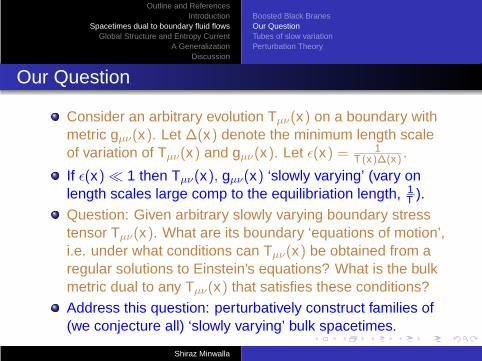
Our Question

Consider an arbitrary evolution Tµν(x) on a boundary withmetric gµν(x). Let ∆(x) denote the minimum length scaleof variation of Tµν(x) and gµν(x). Let ǫ(x) = 1

T (x)∆(x) .

If ǫ(x) ≪ 1 then Tµν(x), gµν(x) ‘slowly varying’ (vary onlength scales large comp to the equilibriation length, 1

T ).

Question: Given arbitrary slowly varying boundary stresstensor Tµν(x). What are its boundary ‘equations of motion’,i.e. under what conditions can Tµν(x) be obtained from aregular solutions to Einstein’s equations? What is the bulkmetric dual to any Tµν(x) that satisfies these conditions?

Address this question: perturbatively construct families of(we conjecture all) ‘slowly varying’ bulk spacetimes.

Shiraz Minwalla





The tubewise approximation

We expect slowly varying boundary configurations to belocally thermalized. Suggests bulk solution tubewiseapproximated by black branes. But along which tubes?Naive guess: lines of constant xµ in Schwarschild (GrahamFefferman) coordinates, i.e. metric approximately

ds2 =dr2

r2f (r)+ r2Pµν(x)dxµ(x)dxν(x) − r2f (r)uµuνdxµdxν

f (r) = 1 −

(

4πT (x)

d r

)d

; Pµν = gµν(x) + uµ(x)uν(x)

Wrong. Metrics not regular. Bad starting point forperturbation theory. Also intuitively problem with causality.

Shiraz Minwalla





Penrose diagram

Finklestein

Boundary

Singularity

Tube

Eddington

Graham FeffermanTube

Future Horizon

PointBifurcation

Shiraz Minwalla





Zero order metric

Causality suggests the use of tubes centered aroundingoing null geodesics. In particular we try

ds2 = g(0)MNdxMdxN = −2uµ(x)dxµdr + r2Pµν(x)dxµdxν

− r2f (r , T (x))uµ(x)uν(x)dxµdxν

Metric generally regular but not solution to Einstein’sequations. However solves equations for constantuµ, T , gµν . Consequntly appropriate starting point for aperturbative soln of equations in the parameter ǫ(x).

Shiraz Minwalla





Perturbation Theory: Redn to ODEs

That is we set

gMN = g(0)MN(ǫx) + ǫg(1)

MN(ǫx) + ǫ2g(2)MN(ǫx) . . .

and attempt to solve for g(n)MN order by order in ǫ.

Perturbation expansion surprisingly simple to implement.Nonlinear partial differential equation → 15 ordinarydifferential equations, in the variable r at each order andeach boundary point.

Shiraz Minwalla





Perturbation Theory: Constraint Equations

Gauge choice: grµ(x) = −uµ(x), grr = 0. Ten

undetermined metric components g(n)µν at each order.

Naively 15 but actually 14 independent Einstein equations.Split up into 4 constraint equations and 10 dynamicalequations.

The constraint equations at nth order are independent ofg(n)

µν : they are ∇µT (n−1)µν = 0, where T (n−1)

µν = 0 is theboundary stress tensor dual to the solution upto (n − 1)th

order.

Shiraz Minwalla





Perturbation Theory: Dynamical Equations

The dynamical equations take the form M g(n) = s(n). HereM is a ‘homogeneous’ differential operator in r that is thesame at every order. s(n) is a source function that isindependent of g(n) and is determined by the solution to(n − 1)th order.

It turns out to be possible to exactly solve the equationM g(n) = s(n) for an arbitrary source function s(n). For anygiven source function sn there is a family of solutions to theequation (which differ by solutions of the homogeneousequation M g = 0)

Shiraz Minwalla





Perturbation Theory: Uniqueness of Solns

However provided that the source function is regular at the‘horizon’ and dies off sufficiently fast at infinity (conditions thatare true for s(n) generated in perturbation theory), the solutionto this equation is unique subject to the following requirements:

1 That the solution is dual to the specified boundary metricgµν(x), velocity field uµ(x) and the temperature T (x).(condition on the large r behaviour of the solution).

2 That the solution is regular at the zeroth order horizon(condition at r = 4πT

d )

Shiraz Minwalla





Perturbation Theory: Navier Stokes Equations

We may now construct the stress tensor T (n)µν dual to our

perturbative solution. T (n)µν is uniquely determined as a

function of nth order in derivatives of gµν , uµ and T .

Recall that the constraint equations are ∇µTµν = 0. Butthis equation, together with the specification of Tµν as afunction of derivatives of gµν , uµ and T has a name: theequations of fluid dynamics.

Shiraz Minwalla





Perturbation Theory: Summary

Summary: Explicit map from the space of solutions of adistinguished set of fluid dynamical equations in ddimensions to long wavelenth solutions of Einstein’sequations.Requirement of regularity of the horizon ensures this mapis locally one to one in solution space.

Naive Graham Fefferman counting: d(d+1)2 − 1 parameter

solution. Rougly parameterized by fluctuation fields gnµν .

However d(d−1)2 − 1 of these modes - the tensor sector -

fixed by the requirement of regularity.Remaining solutions parameterized by d velocities andtemperatures. Closed dynamical system.

Shiraz Minwalla





Explicit Results at second order

We have explicitly implemented our perturbation theory tosecond order.

ds2 = −2uµdxµ (dr + r Aνdxν) + r2gµνdxµdxν

−

[

ωµλωλν +

1d − 2

Dλωλ(µuν) −

1d − 2

Dλσλ(µuν)

+R

(d − 1)(d − 2)uµuν

]

dxµdxν

+1

(br)d (r2 −12ωαβωαβ)uµuνdxµdxν

+ 2(br)2F (br)[

1b

σµν + F (br)σµλσλν

]

dxµdxν . . .

Shiraz Minwalla





Explicit Results at second order

− 2(br)2 σαβσαβ

d − 1PµνK1(br) −

uµuν

(br)d−2

σαβσαβ

(d − 1)K2(br)

+2 L(br)(br)d−2

[

PλµDασα

λuν + Pλν Dασλ

αuµ

]

dxµdxν

− 2(br)2H1(br)[

uλDλσµν + σµλσλν −

σαβσαβ

d − 1Pµν

+Cµανβuαuβ]

dxµdxν

+ 2(br)2H2(br)[

uλDλσµν + ωµλσλν − σµ

λωλν

]

dxµdxν

Shiraz Minwalla





Explicit results at second order

Where

F (br) ≡∫

∞

br

yd−1 − 1y(yd − 1)

dy ; L(br) ≡∫

∞

brξd−1dξ

∫

∞

ξ

dyy − 1

y3(yd − 1)

H2(br) ≡∫

∞

br

dξ

ξ(ξd − 1)

∫ ξ

1yd−3dy

[

1 + (d − 1)yF (y) + 2y2F ′(y)]

K1(br) ≡∫

∞

br

dξ

ξ2

∫

∞

ξ

dy y2F ′(y)2 ; H1(br) ≡∫

∞

br

yd−2 − 1y(yd − 1)

dy

K2(br) ≡∫

∞

br

dξ

ξ2

[

1 − ξ(ξ − 1)F ′(ξ) − 2(d − 1)ξd−1

+(

2(d − 1)ξd − (d − 2))

∫

∞

ξ

dy y2F ′(y)2]

Shiraz Minwalla





Second order boundary stress tensor

The dual stress tensor corresponding to this metric is given by(4πT = b−1d)

Tµν = p (gµν + duµuν)

− 2η[

σµν − τπuλDλσµν − τω

(

σµλωλν − ωµ

λσλν

)]

+ ξσ

[

σµλσλν −

σαβσαβ

d − 1Pµν

]

+ ξCCµανβuαuβ

p =1

16πGd+1bd ; η =s

4π=

116πGd+1bd−1

τπ = (1 − H1(1))b ; τω = H1(1)b ; ξσ = ξC = 2ηb

Shiraz Minwalla





Properties of soln: Stress tensor

Schematic form of 2nd order stress tensor:

Tµν = aT d(gµν + duµuν) + bT d−1σµν + T d−25

∑

i=1

ciSiµν

a is a thermodynamic parameter. b is related to theviscosity: we find η/s = 1/(4π). ci coefficients of the fivetraceless symmetric Weyl covariant two derivative tensorsare second order transport coefficients. Values disagreewith the predictions of the Israel Stewart formalism.Recall that results universal. Should yield correct order ofmagnitude estimate of transport coefficients in any stronglycoupled CFT.

Shiraz Minwalla





Properties of soln: Weyl covariance

Weyl covariance: result is written in terms of covariantderivative built out of the ‘gauge’ field

Aν ≡ uλ∇λuν −∇λuλ

d − 1uν

R. Loganayagam . arXiv:0801.3701 [hep-th]

Can use the fact that Aν transforms like a gauge fieldunder Weyl transformation to define a Weyl covariantderivative D that acts on a weight w tensor Qµ...

ν... as

Dλ Qµ...ν... ≡ ∇λ Qµ...

ν... + w AλQµ...ν...

+[

gλαAµ − δµ

λAα − δµαAλ

]

Qα...ν... + . . .

− [gλνAα − δα

λAν − δαν Aλ] Qµ...

α... − . . .

Shiraz Minwalla




Event Horizons

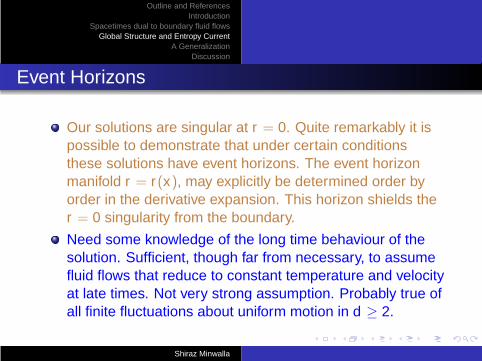
Our solutions are singular at r = 0. Quite remarkably it ispossible to demonstrate that under certain conditionsthese solutions have event horizons. The event horizonmanifold r = r(x), may explicitly be determined order byorder in the derivative expansion. This horizon shields ther = 0 singularity from the boundary.

Need some knowledge of the long time behaviour of thesolution. Sufficient, though far from necessary, to assumefluid flows that reduce to constant temperature and velocityat late times. Not very strong assumption. Probably true ofall finite fluctuations about uniform motion in d ≥ 2.

Shiraz Minwalla




Event Horizon in the derivative expansion

The event horizon of the dual bulk goemetry is the uniquenull manifold that reduces to the event horizon r = 4πT

d = 1b

of the dual uniform black brane at late times.

It turns out to be simple to construct this event horizonmanifold in the derivative expansion: explicitly

rH =1b

+ b(

λ1σαβσαβ + λ2ωαβωαβ + λ3R)

+ . . .

λ1 =2(d2 + d − 4)

d2(d − 1)(d − 2)−

K2(1)

d(d − 1)

λ2 = −d + 2

2d(d − 2)and λ3 = −

1d(d − 1)(d − 2)

Shiraz Minwalla




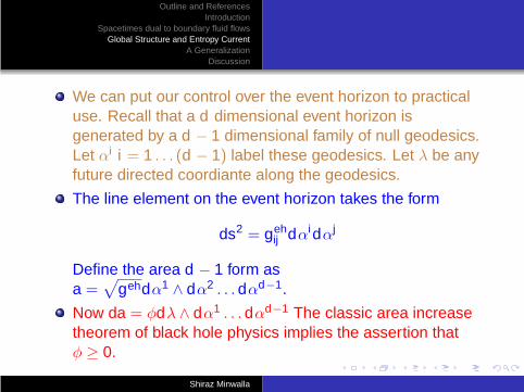
We can put our control over the event horizon to practicaluse. Recall that a d dimensional event horizon isgenerated by a d − 1 dimensional family of null geodesics.Let αi i = 1 . . . (d − 1) label these geodesics. Let λ be anyfuture directed coordiante along the geodesics.

The line element on the event horizon takes the form

ds2 = gehij dαidαj

Define the area d − 1 form asa =

√

gehdα1 ∧ dα2 . . . dαd−1.

Now da = φdλ ∧ dα1 . . . dαd−1 The classic area increasetheorem of black hole physics implies the assertion thatφ ≥ 0.

Shiraz Minwalla




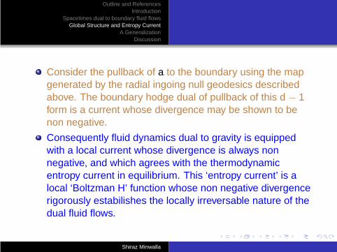
Consider the pullback of a to the boundary using the mapgenerated by the radial ingoing null geodesics describedabove. The boundary hodge dual of pullback of this d − 1form is a current whose divergence may be shown to benon negative.

Consequently fluid dynamics dual to gravity is equippedwith a local current whose divergence is always nonnegative, and which agrees with the thermodynamicentropy current in equilibrium. This ‘entropy current’ is alocal ‘Boltzman H’ function whose non negative divergencerigorously estabilishes the locally irreversable nature of thedual fluid flows.

Shiraz Minwalla




Entropy Current at second order

Explicitly this entropy current is given to second order by

4 Gd+1 bd − 1 JµS = [ 1 + b2 ( A1 σαβ σαβ + A2 ωαβ ωαβ + A3 R ) ] uµ

+ b2 [ B1 Dλ σµλ + B2 Dλ ωµλ ]

where

A1 =2d2 (d + 2) −

K1(1)d + K2(1)

d, A2 = −

12d

, B2 =1

d − 2

B1 = −2A3 =2

d(d − 2)

Shiraz Minwalla




Forcing and Charges

One may attempt to generalize our construction to a bulkLagrangian with additional fields. Gain: more solutions,wider dynamical behaviour. Price: reduced universality

Additional fields of two sorts. Bulk gauge fields thatcorrespond to conserved boundary charge. Plus all others.

Gauge fields enlarge the set of fluid dynamical variables toinclude charge densities. Other fields yield new solns onlywhen non normalizable part is turned on. Operatorcoupling leads to forcing function for fluid dynamics

Shiraz Minwalla




Dilaton Forcing

Example of 2nd kind: d = 4 Einstein Dilaton System.

Long wavelength solution of the Einstein dilaton systemwith a given specified slowly varying boundary dilaton fieldmay be obtained by perturbation theory analogeous toabove. Have been explicitly constructed to second order.

Solutions are in one to one correspondence with the forcedNavier Stokes equations

∇µT µν = −(πT )3

16πG5∇νφ(u.∂)φ + . . .

Shiraz Minwalla




Simple Solutions

A simple class of solutions to these equations are given bythe dilaton chosen as a slowly varying function of time. Ifthe fluid is initially at rest, it stays at rest but slowly heatsup according to

dTdt

=(φ̇)2

12π.

The dual bulk solution has a dilaton pulses falling into theblack hole, and at leading order is the Vaidya solution.Note that varying - whether increasing or decreasing - thedilaton heats up the gauge theory. Consistent with entropy.Speculations about the continuation to weak coupling.

Shiraz Minwalla




Kruskal Coordinates?

Eddington Finklestein coordinates proved very useful forour analysis. One imporant reason: future horizon regularin EF coordinates. Second equally important feature: ∂µ

were killing directions of the black brane, in thesecoordinates. This was crucial for obtaining ODEs - i.e. forthe locality of our solutions.

More generally, our procedure will work once we identifyany foliation of the black brane metric into tubes such that∂a are killing, for the labels a of the tubes. Note too manyoptions. While have not thought this through very carefully,think we have roughly the unique solution

Shiraz Minwalla




Kruskal Coordinates cont

For an example of something that does not work, considerthe black brane written in Kruskal coordinates. If we nowtry to work along lines of constant U or constant V we dontget ODEs, so we dont get tube wise locality

If one wanted to carry out the analouge of our programmein Kruskal coordinates, one would have to solve 2 variablePDEs, and would find locality on sheets not tubes. Thissounds very interesting - though technically difficult. Wouldlove to be able to control such solutions and interpret them.But have had no success so far.

Shiraz Minwalla




Cosmic Censorship ↔ singularities in equilibriation

We have studied gravity dual of a locally equilibriatedtheory. What is the dual of the process of localequilibriation? Clearly the collapse to form a horizon.

Longstanding interesting question about this process: arenaked singularities permitted? Generic? Importantimplications for observational quantum gravity. Appears tomap to questions of singularities in the process of localequilibriation in large N theories. Hint of anotherinteresting connection. Seems like one should study.

Shiraz Minwalla




Finite N

Interesting question in both principle and practice: howdoes this story generalize to finite N. In the bulk one isinstructed to quantize gravity. While this is a formidabletask, it is natural to ask whether it makes any sense tosimply quantize the solutions dual to fluid dynamics.

Technically, one could compute the Witten-Crnkovicsymplectic form on these solutions. If it is finite, welldefined and non degenerate, it would be natural to use it toquantize the phase space of fluid dynamics. Such aquantization would give a ‘wave function’ on the space oftemperatures and velocities (perhaps likely actual storymore complicated). Dual to finite Avagadro no fluctuations?

Shiraz Minwalla




Statistical nature of black hole spacetimes

Clearly the spacetimes we study describe the coarsegrained average properties of some more fundamentaldegrees of freedom. The relation between thesespacetimes and one set of fundamental dofs is dual therelationship between fluid dynamics and gluon positions

What is the relationship between the quantization of thetrue dofs and the quantization of gravity? Perhaps the factthat eternal black holes are dual to spacetimes with twoboundaries is important here.

Shiraz Minwalla




Other issues

Turbulence in gravity

Generalization to confining theories. Boundary dofs.

Time reversal invariance

...

Shiraz Minwalla

Documents

Nonlinear Fluid Dynamics from Gravity-1ism08/talks/SMinwalla.pdf · Global Structure and Entropy Current A Generalization Discussion Large N Dynamics Fluid Dynamics Universal Stress