1

Nonlinear dynamics of locally pulse loaded square Föppl-von 1

Kármán thin plates 2

3

N. Mehreganiana, A. S. Fallahb,c*, L.A. Loucaa 4

a Department of Civil & Environmental Engineering, Skempton Building, South Kensington Campus, Imperial 5

College London, London SW7 2AZ, UK 6

b Department of Mechanical and Aerospace Engineering, Howell Building, Brunel University London, Uxbridge 7

UB8 3PH, UK 8

cICP Institute of Computational Physics, ZHAW Zurich University of Applied Sciences, Technikumstrasse 9, 9

CH-8401 Winterthur, Switzerland 10

11

Abstract 12

13

Modern armour graded thin steel plates benefit from significant elastic strength with high elastic energy 14

storage capacity, which contributes to dissipation of total impulse from extensive blast loads within the bounds 15

of the elastic region. Higher elastic energy storage capability mitigates the probability of catastrophic damage 16

and ensuing large deformations compared to the conventional graded metallic panels. While blast assessment 17

of such structures is important to design and application of protective systems, limited studies are available 18

on their response to localised blasts. 19

The present paper aims at deducing, from the minimization of Föppl-von Kármán (FVK) energy functional, 20

the dynamic response of localised blast loaded thin elastic square plates undergoing large deformations. The 21

presumed blast load function is a multiplicative decomposition of a prescribed continuous piecewise smooth 22

spatial function and an arbitrary temporal function which may assume various shapes (e.g. rectangular, 23

linear, sinusoidal, exponential). 24

A kinematically admissible displacement field and the associated stress tensor were considered as a 25

truncated cosine series with multiple Degrees-of-Freedom (DoF’s). From the prescribed displacement field, 26

having simply supported boundary conditions, useful expressions for stress tensor components were delineated 27

corresponding to a unique mode and a series of differential equations were derived. The explicit solutions were 28

sought using the Poincaré-Lindstedt perturbation method. The closed form solutions of each mode were 29

corroborated with the numerical FE models and showed convergence when the first few modes were 30

considered. The influence of higher modes, however, on the peak deformation was negligible and the solution 31

with 3 DOF’s conveniently estimated the blast response to a satisfactory precision. 32

* To whom correspondence should be addressed:

Email: arash.soleiman-fallah@brunel.ac.uk

Tel.: +44 (0)1895 266408

2

Keywords: Localised blast, Föppl Von-Kármán functional, membrane, Poincaré-Lindstedt method, armour 33

steel, Multiple Degree-of-Freedom Model (MDoF) 34

35

Notations

The following symbols are used in this paper:

Latin upper and lower case 𝑅𝑒 Loading constant (central) zone radius [𝐿]

Greek lower case

𝐴 Elemental area; [𝐿2] 𝛼 Localised blast Load parameter; [1]

𝐿 Plate half-length;[𝐿] ϵ Perturbation parameter; [1]

𝐷 Flexural rigidity; [𝑀𝐿2𝑇−2] 𝜙𝑚𝑛(𝑥, 𝑦, 𝑡) Airy Stress function; [𝑀𝐿𝑇−2]

𝐸 Young’s modulus [𝑀𝐿−1𝑇−2] 𝜙∗(𝑥, 𝑦) Spatial part of Airy Stress function; [1]

𝐻 Plate thickness; [𝐿] �̅�(𝑡) Normalised temporal part of Airy Stress function [1]

𝑊𝑚𝑛(𝑡) Temporal part of the displacement field; [𝐿] 𝜅x,𝜅𝑦 Curvature in x, y direction; [𝐿−1]

𝑎 = 𝑒𝑏𝑅𝑒 Load shape constant; [1]

𝑏 Load shape decay exponent; [𝐿−1] 𝜅𝑥𝑦 Warping curvature; [𝐿−1]

𝑝0 Maximum overpressure; [𝑀𝐿−1𝑇−2] 𝜇 Areal density (= 𝜌𝐻); [𝑀𝐿−2]

𝑝1(𝑥, 𝑦), 𝑝1(𝑟)

Spatial part of pressure pulse load; [𝑀𝐿−1𝑇−2] 𝜌 Material density; [𝑀𝐿−3]

𝑝2(𝑡) Temporal part of pressure pulse load; [1] 𝜃 Polar coordinate rotational angle [1]

𝑤𝑚𝑛∗ (𝑥, 𝑦) Spatial part of the displacement field [L] 𝜈 Poisson’s ratio; [1]

�̅�𝑚𝑛(𝑖)

Normalised maximum mid-point displacement of 𝑖𝑡ℎ iteration [1]

𝜔mn Vibration frequency; [𝑇−1]

𝑡𝑑 Duration of the load; [𝑇] 𝜏𝑚𝑛 Normalised vibration time; [1]

�̅� Pseudo vibration frequency; [𝑇−1]

36

1 Introduction 37

Mitigating the detrimental effects of extensive pulse pressure loads, such as blasts from near 38

field explosives, is crucial due to the catastrophic localised damage to critical equipment and 39

structural elements, as well as potential accompanied loss of life they cause. In the case of a 40

localised blast, structural response is particularly sensitive to the stand-off distance, as the 41

magnitude of blast-induced pressure decays exponentially with the distance between the target 42

and the charge. Hence, localised blast loads impart a focused impulse from the point of projection 43

to the localised regions of the target, leading to large deformations [1]. 44

3

When the deformation of a structural element, such as a thin plate, is of a higher order of 45

magnitude than its thickness, the element undergoes finite displacements (geometry changes) 46

whereby of membrane (catenary) forces are evolved. The membrane forces so emerged will resist 47

out-of-plane deformation and decrease maximum displacement at the cost of high in-plane tensile 48

stresses [2]. 49

Most protective structural systems, such as blast walls, shutters, doors, as well as armored 50

vehicles components, are designed in the form of plated elements. These elements can be 51

fabricated from ductile isotropic materials such as conventional steel or modern armour graded 52

steel with high load bearing capacity beyond the initial yield point, leading to an elastic-plastic 53

response. The former is characterized by a relatively low yield stress and a long plastic plateau 54

while the latter possesses high yield strength and low ductility, whereby the elastic strain energy 55

becomes significant. 56

In fact, for structural systems made of rate-insensitive materials (thus dynamic responses 57

independent of strain rates) and no hardening, the constitutive tensor may be treated as that of 58

elastic-perfectly plastic or rigid-perfectly plastic isotropic metals. As argued by Li et al [3] and 59

Fallah et al [4], when the dimensionless structural response 𝛼 = 𝑅0/𝐾𝑦𝑐 (where 𝑅0, 𝐾, 𝑦𝑐 denote 60

the resistance, stiffness, and critical deformation, respectively) is less than unity and the 61

maximum pulse load 𝑃𝑚 does not exceeds the structural resistance, the rigid-perfectly plastic 62

simplification may not be applicable. In such circumstance, the quotient of the energy stored 63

elastically in the system to the kinetic energy of the plate is noticeable [5]–[7]. 64

Thus, while the elastic response of protective metallic structures against high amplitude 65

dynamic loads is often ignored for simplicity, there are certain cases where such response should 66

be retained in the analysis. Similarly, elastic analysis provides a useful insight into predicting the 67

complex response of quasi-brittle, thin structural plate elements, such as glass panes, composites 68

and thin armour steel. The latter is a suitable candidate material for blast protection as it bears 69

high elastic energy capacity preceding its small plastic deformation[8], [9]. 70

Yuan and Tan examined the response of elastic-perfectly plastic beams to uniform pulse 71

pressure loads by extending the minimum Δ0 technique from Symonds [10]. Three distinct phases 72

of motion were assumed whereby the motion was classified into phase 1- elastic vibration, phase 73

2- perfectly plastic deformation and phase 3- residual elastic vibration. The influence of 74

membrane stretching was only retained at phase 3 when the motion was characterised by 75

travelling plastic hinges. Thus, the elastic and plastic responses were distinctly separated in each 76

phase of motion, whilst the membrane stretching effects in the elastic regime was ignored. 77

4

The present study deals with applying the well-established Föppl Von-Kármán model to 78

address the influence of finite displacement, or geometry changes in the overall response of the 79

structure, in light of the developed membrane resistance in conjunction with the bending 80

resistance of the structure. 81

In fact, the FVK model is particularly pragmatic to capture the pronounced variation of shell 82

transverse deformation field with its membranal strains using the minimal geometric 83

nonlinearity [11]. The scientific literature devoted to applications of this model spans from 84

buckling and post-buckling of plates in aerospace engineering [12], [13] to blast response of 85

laminate glass [14]–[16], from instabilities of composites under thermal loads [17] to wrinkling 86

of soft biological tissues[18]. Recently, in the fields of aerospace, structural and mechanical 87

engineering, the complex response of plates to blast loads of distinct types has been highlighted 88

the limitations of classical theories and the need for consideration of geometric nonlinearities 89

using the FVK model. This is particularly essential for structures where the contribution of the 90

energy stored elastically through the plate to the total kinetic energy cannot be ignored. An 91

example of this is the counter-intuitive behaviour of armour steel compared to conventional steel 92

graded panels which ruptured at the same impulse despite the lower ductility and midpoint 93

transverse deflection. [9]. 94

Teng et al [19] examined the transient deflection of the simply supported and clamped square 95

plates under a uniform blast load with exponentially decaying time function. The FVK expressions 96

were reduced to Duffing equations using the variational techniques. The authors employed the 97

Poincaré-Lindstedt perturbation method to analyse the plate response. While the transient 98

deformation at the first approximation was concurrent with that of numerical models, prediction 99

of the response was limited to the loading phase only. Feldgun et al. [20] developed an SDOF 100

model for rectangular plates with various boundary conditions subjected to a uniformly 101

distributed exponential pulse load. Static and dynamic analyses were developed and compared 102

with the numerical models as well as the available experimental tests. However, the plot of 103

deformation time history determined from the numerical solution of Duffing equation, using the 104

Runge-Kutta method, revealed the increase in peak deformations over time. Any theoretical or 105

numerical treatment of the problem of this kind should be couched in caveats, as the presence of 106

secular terms (such as 𝑡𝑠𝑖𝑛(𝑡)) would lead to unbounded growth of deformations and would not 107

reflect the actual response of the structure. A similar phenomenon was observed in [21] which 108

used Ultraspherical Polynomial Approximation technique on circular and square plates with 109

various boundaries. 110

5

For high-dimensional nonlinear dynamic systems, due to the existence of modal interactions, 111

different forms of vibrations may arise as a consequence of relationship between several types of 112

internal resonant cases. A special internal resonant relationship between two linear natural 113

frequencies may lead to large amplitude nonlinear response [22]. Wang et al [23] studied the 114

transient response of doubly curved graphene nanoplatelet reinforced composite (GPLRC) shells 115

upon the thermal effects of the blast loads. Based on Reddy’s higher order shear deformation 116

theory [24] and von Kármán’s strain displacement expressions, a growth in the vibration 117

amplitude with the increase in pulse duration, while diminishing the response frequency, is 118

observed. Similarly, the temperature difference between the top and bottom surfaces of the 119

GPLRC induced permanent transverse deformation on the shell. Liu et al [22] and Zhang et al [25], 120

in parallel studies, investigated the visco-elastic response of composite laminated circular 121

cylindrical shells with pre-stretched membranes due to periodic thermal effects. Based on the 122

third order shear-deformation theory, Galerkin’s method and Poincaré’s perturbation theory, the 123

periodic and chaotic motions were observed depending on the temperature variation in the 124

interval of 15-70oK/oC. Zhang et al [26] used the same theory to study the chaotic motion of 125

orthotropic plates due to transverse and in-plane excitations. The existence of chaotic response 126

was confirmed for certain transverse excitations. 127

Linz et al [14] presented experimental and numerical studies on the performance of 128

laminated glass subjected to uniform blast loads. The Material properties (average stiffness, 129

Poisson’s ratio and average areal density) of the full composite action were estimated as an 130

average of the properties of each lamina (consisting of glass and Polyvinyl Butyral (PVB)). The 131

analytical model employed FVK expressions to capture the PVB membranal forces and maximum 132

deformations. The authors assumed a truncated series of cosine functions to represent the 133

displacement field of the structure. The assumption of using a single term for the deformation 134

and Airy stress function series pragmatically estimated the response for the lower intensity blasts 135

to characterize the pre-crack behaviour of the composites. However, the Digital Imaging 136

Correlation from experiments showed that such a deflection shape would not be suitable for more 137

intense loading. The curvature field from DIC was non-uniform with curvature concentration on 138

the plate edges. However, the analytical model was sparse, i.e. the post loading behaviour of the 139

plate was not investigated analytically. Clearly, the transient pulse loading induced dynamic 140

response is a two-step process which consists of an undamped forced- and free-vibration, the 141

latter occurring beyond fluid-structure separation. The visco-elasticity (damping effects) would 142

not contribute to the elastic energy dissipation due to the short duration response although it 143

kills it off in the subsequent cycles. 144

6

Over the past decades, the literature concerned with the performance of structures subject to 145

blast loads have mostly dealt with pulse pressures of uniform distribution across the target, 146

which is pertinent to the blasts charges with stand-offs more than the half-span of the structural 147

element [27]. However, the physics of localised blast is complex as the response is contingent 148

upon, and sensitive to, the load parameters characterising the spatial and temporal distribution 149

of the dynamic pressure. 150

Thus, the objective of this work is to examine the explicit solutions of geometrically nonlinear 151

elastic, isotropic homogeneous square plate to localised blast load. The plates investigated here 152

are assumed thin, where the terms of transverse shear from the Mindlin-Reisner plate theory can 153

be neglected, but as the blast loads incur damage and deformation in high order of the plate 154

thickness, the influence of finite displacements, or geometry changes, due to the presence of 155

membranal forces must be retained in the analysis conducted. This is achieved by implementing 156

the well-known Föppl-Von Kármán (FVK) nonlinear theory. 157

The current paper is organized in 6 sections and entails a description of the localised blast in 158

section 1, followed by the derivation of the governing equations of membrane elasticity in section 159

2. In Section 3, the theoretical solutions at two distinct phases of motion are investigated, while 160

the pulse shape effects were examined in section 4. The theoretical solutions were validated 161

against the Finite Element numerical models in Section 5. Finally, the concluding remarks of the 162

study are presented in Section 6. 163

1.1 Localised blast load 164

165

Typical blasts associated with chemical exothermic reactions rapidly release a significant 166

amount of energy which generates an overpressure, i.e. pressure beyond the atmospheric 167

pressure, at a given stand-off distance followed by monotonic decay back to the ambient pressure. 168

A wide range of experimental data by Kingery and Balmash provided reference to describe the 169

air blast parameters through empirical equations. The empirical relations represented the blast 170

load parameters of given TNT equivalent charge using the Hopkinson-Cranz scaling parameter. 171

However, these data were limited to the range of parameters investigated, while the blast wave 172

interaction with the target was restricted to infinite reflecting surfaces (no reflection) [28], [29]. 173

The blast load function in this study is truncated into a single term of multiplicative 174

decomposition of its temporal (pulse shape) and spatial (load shape) functions. The load shape 175

parameters depend on the proximity of the blast source whilst the pulse shape is influenced by 176

the characteristics of the blast source, namely as either deflagration, such as gas explosion giving 177

7

rise to a pulse shape with finite rise time depending on the stoichiometric composition of the 178

ambience, or detonation (high explosives explosion with virtually zero rise time and 179

exponentially decaying pulse shape). The pulse shape has no intrinsic effect on the response for 180

impulsive blasts, i.e. when loading duration is small (𝑡𝑑 → 0). In such circumstances, the pressure 181

would be idealised with Dirac delta function. The assumed spatial variation of the load, as shown 182

by Eq. (1) and in Fig. 1, maintains a uniform pressure within the central disk of radius 𝑟𝑒 before 183

decaying exponentially along radial coordinate (𝑟) [2], [8], [30]–[32]. We also examine the 184

influence of pulse shape and show the significant difference between the response due to various 185

pulse shapes for a purely elastic body. 186

In fact, the literature on the pulse shape profiles and pressure time histories is rich. Schleyer 187

and Hsu [33] presented an experimental study of dynamic pressure load type of confined gas 188

explosions. The plate resisted the loading primarily by elastic membrane and no noticeable yield 189

line/plastic hinges were formed. Aune et al. [29], [34] presented studies on the response of 190

aluminium alloys based on experimentally obtained pressure time-history data using the Digital 191

Image Correlation (DIC) technique. Yuan and Tan discussed Youngdahl’s technique [35], [36] to 192

eliminate the pulse shape influence to be valid only for monotonically decaying pulse [37]. 193

The plated structure studied here comprises an initially flat, monolithic, ductile metallic 194

square plate with side length 2𝐿, thickness of 𝐻 and areal density of 𝜇 = 𝜌𝐻. The plate is secured 195

along its periphery with simply supported boundary conditions and subject to a localised pulse 196

pressure load. Thus, the load is axisymmetric and reduces the domain of study to only one quarter 197

of the plate (considering the square plate has 4 axes of symmetry). 198

Fig. 1- Spatial distribution of load

199

8

𝑝1(𝑟) = {𝑝0 0 ≤ 𝑟 ≤ 𝑅𝑒

𝑝0𝑎𝑒−𝑏𝑟 𝑅𝑒 ≤ 𝑟 ≤ 𝑅 (1)

𝑝2(𝑡) = {1 𝑓𝑜𝑟 0 ≤ 𝑡 ≤ 𝑡𝑑 0 𝑓𝑜𝑟 𝑡 ≥ 𝑡𝑑

(2)

For simplicity, the negative phase of the pulse load is ignored as its influence is deemed 200

negligible in the event of localised blasts. Using the Ritz-Galerkin’s method, load functional is 201

minimised in Eq. (3). The load is rotationally symmetric, thus independent of the polar coordinate 202

𝜃. Hence, while the integral may be easily evaluated for two asymptotic cases, i.e. considering (i) 203

the square plate of half-length 𝐿 equal to that of a circular one with radius 𝑅, and (ii) the radius 204

being 𝑅 = √2𝐿. The actual value is bounded between the two. In fact, the difference between the 205

evaluated integrals for the two cases in most scenarios is infinitesimal and may be ignored. For 206

accurate evaluation of the actual integral by implementing the transformation of coordinates, 207

such a functional may be furnished into a single dimensionless parameter 𝛼 in Eq. (4), influenced 208

by the central constant load radius 𝑅𝑒 as well as the load decay exponent 𝑏, expressed. 209

∫∫ 𝑝(𝑥, 𝑦, 𝑡)𝛿𝑤𝑑𝐴(𝐴)

= ∫∫ 𝑝0 cos (𝜋𝑥

2𝐿) cos (

𝜋𝑦

2𝐿)𝑑𝑥𝑑𝑦

𝐴

+ ∫∫ 𝑝1(𝑥, 𝑦) cos (𝜋𝑥

2𝐿) cos (

𝜋𝑦

2𝐿) 𝑑𝑥𝑑𝑦

𝐴

= ∫ ∫ 𝑝0 cos (𝜋𝑟𝑐𝑜𝑠(𝜃)

2𝐿) cos (

𝜋𝑟𝑠𝑖𝑛(𝜃)

2𝐿) 𝑟𝑑𝑟𝑑𝜃

𝑅𝑒

0

𝜋2

0

+ ∫ ∫ 𝑝0𝑒−(𝑏𝑟−𝑏𝑅𝑒) cos (

𝜋𝑟𝑐𝑜𝑠(𝜃)

2𝐿) cos (

𝜋𝑟𝑠𝑖𝑛(𝜃)

2𝐿) 𝑟𝑑𝑟𝑑𝜃

𝐿

𝑅𝑒

𝜋2

0

= 𝛼𝑝0𝐿2

(3)

210

Fig. 2- Influence of the load parameters on the value of 𝜶 with 𝑳 = 𝟎. 𝟐

9

It can be seen in Fig. 2 that various values of 𝛼 converge to a unique value pertinent to the 211

case of uniformly distributed load as 𝑅𝑒 → 𝐿 , independent of the decay type. 212

α =1

𝑏2𝐿2(2𝐿2𝑏2 + 𝜋2)2[32((

1

16𝜋4𝑏𝑅𝑒 +

1

4𝐿2𝑏2(𝑏𝑅𝑒 + 3)𝜋2 + 𝐿4𝑏4) 𝑐𝑜𝑠 (

𝜋𝑅𝑒

2𝐿)

+1

2𝜋𝑏𝐿 ((

1

4𝑏𝑅𝑒 −

1

2)𝜋2 + 𝐿2𝑏3𝑟𝑒) 𝑠𝑖𝑛 (

𝜋𝑅𝑒

2𝐿)

+1

8𝜋3 (𝑏2𝐿2 + 2𝐿𝑏 +

1

4𝜋2) 𝑒−𝑏(𝐿−𝑅𝑒) − (𝑏2𝐿2 +

1

4𝜋2)

2

)]

(4)

2 Governing Equations 213

The general expression for the Cartesian components of the strain tensor is given as: 214

휀𝑖𝑗 =1

2(𝑢𝑖,𝑗 + 𝑢𝑗,𝑖 + 𝑢𝑘,𝑖𝑢𝑘,𝑗) (5)

where 𝒖(𝑥𝑖, 𝑡) is the displacement field and the comma in subscripts denotes differentiation 215

with respect to the coordinate that follows, i.e. 𝑢𝑖,𝑗 = 𝜕𝑢𝑖/𝜕𝑥𝑗. For convenience, the components 216

of tensors, in the reference space in indicial notation 𝒞(𝑖, 𝑗, 𝑘) may be replaced by those in von 217

Kármán notation 𝒞(𝑥, 𝑦, 𝑧). Thus, given the Cartesian coordinates (𝑥, 𝑦) on 𝒞 centred at its 218

centroid, the components of displacement are: in plane 𝑣𝑖 = (𝑣𝑥, 𝑣𝑦) , and transverse 𝑤. The 219

components of the strain tensor and the curvature terms, using the reciprocity conditions (𝑎𝑖𝑗 =220

𝑎𝑗𝑖) read: 221

휀𝑥 =𝜕𝑣𝑥

𝜕𝑥+

1

2(

𝜕𝑤

𝜕𝑥)

2

, 휀𝑦 =𝜕𝑣𝑦

𝜕𝑦+

1

2(

𝜕𝑤

𝜕𝑦)

2

,

(6a-c)

𝛾𝑥𝑦 =𝜕𝑣𝑥

𝜕𝑦+

𝜕𝑣𝑦

𝜕𝑥+

𝜕𝑤

𝜕𝑦

𝜕𝑤

𝜕𝑥

𝜅𝑥 = −𝜕2𝑤

𝜕𝑥2, 𝜅𝑦 = −

𝜕2𝑤

𝜕𝑦2, 𝜅𝑥𝑦 = −

𝜕2𝑤

𝜕𝑥𝜕𝑦 (7)

The second term in Eq.’s (6a-c) represent the membrane strains whose associated 222

deformation gradients are the sole contributors to geometric nonlinearity. The compatibility 223

condition of strains is given by the following equation pair: 224

𝜕2휀𝑥

𝜕𝑦2+

𝜕2휀𝑦

𝜕𝑥2−

𝜕2𝛾𝑥𝑦

𝜕𝑥𝜕𝑦= 𝜅𝑥𝑦

2 − 𝜅𝑥𝜅𝑦 = −det 𝑘 (8)

∇ × 𝑘 = 0 (9)

10

Eq. (8) represents the Gaussian invariant curvature (Gauss Theorema Eregium). The FVK 225

Equations giving the fundamental description of nonlinear elastic dynamics of the thin plate 226

reads: 227

𝐷∇4𝑤(𝑥, 𝑦, 𝑡) − 𝐻ℒ(𝑤,Φ) = 𝑝(𝑥, 𝑦, 𝑡) (10)

∇4Φ(𝑥, 𝑦, 𝑡) = −𝐸

2ℒ(𝑤,𝑤) ⟺ −𝐸(𝜅x𝜅𝑦 − 𝜅𝑥𝑦

2 ) (11)

Thus, the Gaussian curvature is quadratic with respect to the transverse displacement field. 228

Eq. (11) is a compatibility equation, where Φ(𝑥, 𝑦, 𝑡) represents the Airy stress function, 𝐷 =229

𝐸𝐻3

12(1−𝜈2) is the flexural rigidity of the plate, the biharmonic operator ∇4 and the differential 230

operator ℒ(𝑤,Φ) are expressed by Eq.’s (12) and (13), respectively. 231

∇4Φ =𝜕4Φ

𝜕𝑥4+ +2

𝜕4Φ

𝜕𝑥2𝜕𝑦2+

𝜕4Φ

𝜕𝑦4

(12)

ℒ(𝑤,Φ) =𝜕2𝑤

𝜕𝑥2

𝜕2Φ

𝜕𝑦2+

𝜕2𝑤

𝜕𝑦2

𝜕2Φ

𝜕𝑥2− 2

𝜕2𝑤

𝜕𝑦𝜕𝑥

𝜕2Φ

𝜕𝑥𝜕𝑦 (13)

The Airy stress function represents the membrane action induced by large displacements and is 232

defined by: 233

𝜎11 =𝜕2Φ

𝜕𝑦2, 𝜎22 =

𝜕2Φ

𝜕𝑥2, 𝜎12 = −

𝜕2Φ

𝜕𝑥𝜕𝑦 (14)

Eq. (11) is a compatibility equation as discussed earlier, while ℒ(𝑤,𝑤)can also be expressed 234

by replacing Φ with 𝑤 in Eq. (13). Eq.’s (10)- (13) are coupled, highly nonlinear, fourth order 235

Partial Differential Equations (PDE) which represent geometric nonlinearities of an elastic 236

system induced by in-plane displacements and membranal forces. It is well known that even for 237

simple engineering problems, the exact solution of FVK equations are notoriously difficult to 238

obtain thus, in general, a numerical solution must be adopted. In the case of localised blast loads, 239

the equations are fraught with more complexity due to the dependence of the load on the spatial 240

and temporal multi-variables. Minimization of the FVK energy functionals calls for numerical 241

Finite Element techniques, boundary elements, meshless methods, or some efficient variational 242

method such as Ritz-Galerkin (RG). The approach resorted to herein seeks to reduce the PDE to a 243

set of Ordinary Differential Equations (ODE’s) using the Poincaré-Lindstedt (P-L) perturbation 244

technique, combined with the RG method. 245

The mathematical procedure for such shell elements is outlined as follows: 246

11

1. Assume an ansatz for displacement fields and the associated stress tensors. 247

2. Determine the membranal stress from the compatibility relation of Eq. (13). 248

3. Update the displacement field from Eq. (10). 249

4. The final form of transverse displacement will be nonlinear, but in a reduced closed 250

form expression. 251

The ansatz for displacement field and the associated stress functions may be expressed as 252

multiplicative decomposition of their functions describing the spatial part as well as that of the 253

temporal part, i.e. 𝑤𝑚𝑛(𝑥, 𝑦, 𝑡) = 𝐻�̅�𝑚𝑛(𝑡)𝑤∗(𝑥, 𝑦) and 𝜙𝑚𝑛(𝑥, 𝑦, 𝑡) = 𝑓(𝑡)𝜙∗(𝑥, 𝑦), respectively, 254

where the partial functions 𝑤∗(𝑥, 𝑦) and 𝜙𝑚𝑛∗ (𝑥, 𝑦) are expressed by Eq.’s (15)-(16). Accordingly, 255

the dimensionless parameters �̅� = 𝑓(𝑡)/𝐸𝐻2, and �̅�𝑚𝑛(𝑡) = 𝑤𝑚𝑛(0,0, 𝑡)/𝐻 have been employed. 256

Clearly, these expressions satisfy the displacement boundary conditions of the simply supported 257

plate at its centre as well as along its periphery. 258

𝑤∗(𝑥, 𝑦) = ∑ ∑ cos𝑚𝜋𝑥

2𝐿cos

𝑛𝜋𝑦

2𝐿𝑛𝑚 (15)

𝜙∗(𝑥, 𝑦) = ∑ ∑ cos𝑚𝜋𝑥

2𝐿𝑛𝑚cos

𝑛𝜋𝑦

2𝐿

(𝑚 = 1,3,5, … 𝑎𝑛𝑑 𝑛 = 1,3,5, … )

(16)

The RG technique to minimize the total elastic energy functional can be sketched in Eq.’s (17a-259

b). With this strategy, we may, dynamically update the interrelation between the transverse 260

displacement field in Eq. (17a) from the state of membranal stress tensors satisfying Eq. (17b), 261

and vice versa. 262

∫∫ {𝐷∇4 �̅�(i+1)

(𝐴)

− 𝐻3𝐸ℒ(w̅(i), Φ̅(i+1)) + 𝜇�̅�..

(i+1) }𝛿𝑤𝑑𝐴 = ∫∫𝑝(𝑥, 𝑦, 𝑡)

𝐻𝛿𝑤𝑑𝐴

(𝐴)

(17a)

∫∫ {∇4Φ̅(i+1) +1

2ℒ(w̅(i), w̅(i))} 𝛿Φ

(𝐴)

𝑑𝐴 = 0 (17b)

In Eq. (17a)- 𝛿𝑤 and 𝛿Φ represent the first variation (virtual parameter, or weight function) 263

attributed to the displacement and Airy stress functions, respectively, while the superscript 264

denotes the iteration. Substituting Eq.’s (15)-(16) in Eq. (17) furnishes the bending and strain 265

energy contributors into: 266

12

ℒ(�̅�, ϕ̅) =1

32

𝜋4

𝐿4𝑚2𝑛2 ∑ ∑ �̅�𝑚𝑛(𝑡)ϕ̅𝑚𝑛 (cos

𝑚𝜋𝑥

𝐿+ cos

𝑛𝜋𝑦

𝐿)

𝑛𝑚 (18)

∇4�̅� =1

16

𝜋4

𝐿4(𝑚2 + 𝑛2)2 ∑ ∑ �̅�𝑚𝑛(𝑡) cos

𝑚𝜋𝑥

2𝐿𝑛cos

𝑛𝜋𝑦

2𝐿𝑚 (19)

The operator ℒ(�̅�, �̅�) and the biharmonic function ∇4Φ̅ may be recovered, in a similar 267

fashion, by simply replacing Φ̅ with �̅� in Eq. (18) and vice versa in Eq. (19). Assuming the Von-268

Mises yield criterion (𝐽2-plasticity), the Equivalent Mises stress is expressed as a function of the 269

components of the deviatoric stress tensor as follows: 270

𝜎𝑒𝑞 =3

2√𝑠𝑖𝑗𝑠𝑖𝑗 = √3𝐽2 (20)

Where 𝑠𝑖𝑗 = 𝜎𝑖𝑗 − 𝒑𝛿𝑖𝑗 are the components of the deviatoric stress tensor (𝒑 = 𝜎𝑘𝑘 3⁄ ), and 𝐽2 271

is the second invariant of the deviatoric stress tensor and may be derived by substituting Eq.’s (A. 272

45)-(A. 47) in Eq. (21) (with 𝜎33 = 0) as: 273

𝐽2 =1

3(𝜎11

2 + 𝜎222 − 𝜎11𝜎22 + 3𝜎12

2 ) (21)

The associated Equivalent Mises strains are likewise derived as: 274

휀𝑒𝑞 =1

3√6ε11

2 + 6ε222 + 3ε12

2 (22)

Throughout this work, ARMOX 440T steel has been used as the candidate material with the 275

material properties outlined in Table 1, as well as the geometric dimensions of the membrane. 276

Table 1 Constants used in this study 277 Load parameters Geometric and material properties

𝑏

(𝑚−1) 𝑝0

(MPa)

𝐿

(𝑚𝑚) 𝐻

(𝑚𝑚) 𝜈 𝐸

(𝐺𝑃𝑎) 𝜌

(𝑘𝑔.𝑚−3) 50 40/200 200 4.6 0.3 200 7850

278

3 Dynamic Response 279

3.1 First Phase of Motion (Forced Vibration) 280

Now, substituting Eq.’s (18)-(19) in Eq.’s (17a-b) and performing the integrations reduces the 281

form of FVK Partial Differential Equation to a paired set of 𝑚 × 𝑛 ODE’s in terms of the transverse 282

displacement fields, each representative of a unique mode shape of the MDOF system in forced 283

vibration. While coupling between the modes is retained in the analysis, for the brevity in the 284

13

mathematical treatment, only the first four terms of the truncated series (i. e.𝑚 = 𝑛 = 1,3) may 285

be considered. The set of ODE’s were derived as 286

𝜔mn2 �̅�𝑚𝑛

(𝑖+1) + �̅�..

𝑚𝑛

(𝑖+1)+

9𝐸𝜋2𝜖

8𝜌𝐿2𝑺(𝒎𝒏)𝐬𝟏

(𝑖) �̅�𝟏𝐤(𝑖+1)

δ′sk =4𝛼𝑝0

ρ𝐻2 (23)

where 𝜖 =8

9𝐻2/𝐿2 is a parameter of small value, while the matrices 𝑺(𝒎𝒏)𝑠1 and �̅�𝟏𝐤

(𝑖+1) are 287

defined in Eq.’s (24a-b), and δ′sk is the Kronecker Delta. Then, for each displacement field term 288

�̅�𝑚𝑛, the associated components of the matrix 𝑩𝑚𝑛 are expressed in Eq.’s (A-48)-(A-50). From 289

the compatibility Eq. (17b) the components of �̅�1𝑘(i+1)

in Eq. (23) with 𝑖 = 1 can be unequivocally 290

determined as in Eq.’s (A. 51)-(A. 53). In the absence of higher order terms, �̅�11(2)

= −4

3𝜋2 �̅�11(𝑖)2

and 291

the solution converges to the case of an SDOF system. 292

𝑺(𝒎𝒏)𝑠1(i) = 𝑩𝑚𝑛[�̅�11

(𝑖) �̅�13(𝑖)�̅�31

(𝑖)�̅�33(𝑖)]′, �̅�1𝑘

(𝑖+1) = [�̅�11

(i+1)�̅�13

(i+1)�̅�31

(i+1)�̅�33

(i+1) ]. (24a-b)

It should be noted that, each ODE in Eq. (23) correspond to a mode of vibration with the mode 293

coupling appearing in the nonlinear term �̅�1𝑘(i+1)

. The coefficients of �̅�1𝑘(i+1)

may be visualized as 294

the equivalent membrane stiffness of the plate while the vibration frequency 𝜔𝑚𝑛2 gives the ratio 295

of the bending stiffness to the equivalent mass of the structure. Thus, the vibration frequency ω𝑚𝑛 296

is determined as: 297

ω𝑚𝑛 =1

4

𝜋2

𝐿2(𝑚2 + 𝑛2)√

𝐷

𝜇=

√3

24

𝜋2𝐻

𝐿2(𝑚2 + 𝑛2)√

𝐸

𝜌(1 − 𝜈2) (25)

confirming that the modal vibration frequencies uniquely depend on the speed of dilatational 298

wave propagation through the plate as well as its slenderness ratio. Clearly, each of the ODE’s of 299

Eq.(23) is an inhomogeneous, expanded form of Duffing equation [38]. If the high order 300

transverse displacement terms are ignored, using the separation of variables, the closed form 301

explicit solution of this ODE can be expressed as (�̅�.2 = ℎ +

8𝛼𝑝0

𝜇𝐻�̅� − [𝜔11

2 �̅�2 +𝐸

2𝜌𝐿2 ϵ�̅�4], where 302

ℎ is the integration constant) with the left hand side representing the normalised kinetic energy 303

per mass of the system. If ϵ is positive, the force-displacement gradient increases and the system 304

represents hardening [20], in which case the plane plot encompasses an elliptic manifold, as is 305

the case here (as illustrated in Fig. 3), while in the circumstances of negative ϵ the softening of the 306

stiffness would occur. 307

14

Fig. 3- Phase plane for various values of 𝒕𝒅, where 𝑻𝒇 is an arbitrary time

point

Heuristically, with the nonlinear terms present in the Eq. (23), the explicit solution entails the 308

presence of secular terms (in the form of 𝑡 sin(𝑡)) which bring about a non-harmonic response 309

with unbounded growth of transient displacements. The solution can be made harmonic by 310

employing the Poincaré-Lindstedt perturbation method to eliminate, once and for all, the 311

dependence of the displacement field on such terms. To this end, the frequency response is 312

normalised as 𝜏𝑚𝑛 = (𝜔𝑚𝑛 + 𝜖�̅�𝑚𝑛 + 𝑂(𝜖2)), where �̅�𝑚𝑛 is referred to as the pseudo vibration 313

hereinafter. Accordingly, the displacement field is expressed as a truncated series of its iterative 314

terms given by: 315

�̅�𝑚𝑛(𝜏𝑚𝑛) = �̅�𝑚𝑛(1)(𝜏𝑚𝑛) + 𝜖�̅�𝑚𝑛

(2)(𝜏𝑚𝑛) + 𝑂(𝜖2) (26)

The solution to the first iteration �̅�𝑚𝑛(1) is derived by linearizing the form of the ODE in Eq. 316

(23), i.e. eliminating the Airy Stress function terms 𝑸1k(1)

. The general solution of the system must 317

satisfy the initial kinematic conditions �̅�(0) = �̅�.(0) = 0, and can be sketched as: 318

�̅�𝑚𝑛(1)

= 𝑐𝑚𝑛(1 − cos(𝜔𝑚𝑛𝑡)) (27)

where the amplitude of vibration is 319

𝑐𝑚𝑛 =4𝛼𝑝0

𝜇𝐻𝜔𝑚𝑛2

(28)

To derive the ODE expression for the second term, we shall henceforth ignore the terms of 320

higher order as 𝜖2 << 1. Substituting Eq. (26) in Eq. (23)together with the use of Eq. (27) yields 321

15

𝜔12(�̅�(2)

𝑚𝑛 + �̅�..

(2)𝑚𝑛) + 2ω𝑚𝑛�̅�1𝑐𝑚𝑛�̅�

..(1)

𝑚𝑛 +9𝐸𝜋2

8𝜌𝐿2𝑺𝑚𝑛𝑠1

(𝟏) �̅�1𝑘

(2)δ′sk = 0

(29)

From Eq. (27) the second iteration for the Airy Stress function at the plate centre is attained. 322

Sequentially, the ODE of Eq. (23) is re-evaluated and solved to determine, unequivocally by 323

imposing the initial boundary conditions, the plate maximum transverse displacement as: 324

�̅�11(1)

= (2.2𝐸𝑐11

3

𝜔112 𝐿2𝜌

−𝑐11�̅�1

𝜔11

) 𝑠𝑖𝑛(𝜏11)𝜏11

+𝑐113𝐸

𝐿2𝜌𝜔12{ −0.0347𝑐𝑜𝑠(𝜏11)

15 + 0.1302𝑐𝑜𝑠(𝜏11)13 − 0.273𝑐𝑜𝑠(𝜏11)

11

+ 0.109𝑐𝑜𝑠(𝜏11)10 + 0.335𝑐𝑜𝑠(𝜏11)

9 − 0.274𝑐𝑜𝑠(𝜏11)8 − 0.282𝑐𝑜𝑠(𝜏11)

7

+ 0.471𝑐𝑜𝑠(𝜏11)6 − 0.0861 cos(𝜏11)

5 − 0.297𝑐𝑜𝑠(𝜏11)4 + 0.118𝑐𝑜𝑠(𝜏11)

3

+ 1.13𝑐𝑜𝑠(𝜏11)2 + 2.52𝑐𝑜𝑠(𝜏11) − 3.5664}

(30)

�̅�11 =2.2𝐸𝑐11

2

𝐿2𝜔1𝜌 (31)

where the derived parameter �̅�1 in Eq. (31), determined by the first bracket of Eq. (30), 325

eliminates the secular term and to make the response periodic. Further iterative components of 326

Airy stress matrix function �̅�1𝑘(i) may be evaluated by substituting Eq.’s (30),(32), and (33) in each 327

of the Eq.’s (A. 51)-(A. 53). 328

In a similar fashion, the expressions for �̅�13(2)

and �̅�33(2)

are determined as Eq.’s (32) and (33). 329

It is interesting to note the infinitesimal disparity between the values of �̅�𝑖𝑗 in the associated 330

higher modes to that of the fundamental mode. For example, the value of �̅�13 is only 2.4% lower 331

than �̅�11. 332

�̅�13(1)

= (6710𝑐13

2 𝐸

𝐿2𝜌 𝜔132 −

�̅�13

𝜔13

) 𝑐13𝑠𝑖𝑛(𝜏13)𝜏13

+𝐸𝑐13

3

𝐿2𝜌𝜔132 (6.98𝑠𝑖𝑛 (

3

2𝜏13)

2

− 6730𝑠𝑖𝑛 (1

2𝜏13)

2

+ 58720𝑠𝑖𝑛 (1

5𝜏13)

2

+ 46110𝑠𝑖𝑛 (2

5𝜏13)

2

− 37730𝑠𝑖𝑛 (3

5𝜏13)

2

− 143150𝑠𝑖𝑛 (1

10𝜏13)

2

− 16590𝑠𝑖𝑛 (3

10𝜏13)

2

+ 3740𝑠𝑖𝑛 (7

10𝜏13)

2

+ 248.44𝑠𝑖𝑛 (9

10𝜏13)

2

+ 144.92 𝑠𝑖𝑛 (11

10𝜏13)

2

− 482.67𝑠𝑖𝑛(𝜏13)2)

(32)

16

�̅�33(1)

= 𝑐11

3 𝐸

𝐿2𝜔332 𝜌

(−0.106𝑐𝑜𝑠(𝜏33) + 0.882 − 0.105𝑐𝑜𝑠 (10

3𝜏33) − 0.897𝑐𝑜𝑠 (

10

9𝜏33)

− 0.0799𝑐𝑜𝑠 (11

9𝜏33) − 0.186𝑐𝑜𝑠 (

7

9𝜏33) − 0.449𝑐𝑜𝑠 (

2

3𝜏33)

+ 0.741𝑐𝑜𝑠 (2

9𝜏33) + 0.619𝑐𝑜𝑠 (

5

9𝜏33) + 0.477𝑐𝑜𝑠 (

8

9𝜏33) − 0.318𝑐𝑜𝑠 (

4

9𝜏33)

+ 0.3759cos (𝜏33)

(33)

333

(a) (b)

Fig. 4- Comparison of modal deformations histories in the first phase of motion, for (a) second and

third mode, (b) first and second mode

It can be seen in Fig. 4 that the influence of higher modes on the overall transient response of 334

the structure is inconsequential. Thus, the mathematical treatment of elastic systems with merely 335

two terms of the truncated series renders the overall response sufficiently accurate. 336

337

3.2 Second Phase of Motion (Free Vibration) 338

The loading is complete at time 𝑡 = 𝑡𝑑; however, the system retains its motion due to the 339

initial inertia effects and the energy stored in it. Thus, the associated response of the plate is 340

governed by a free vibration following the forced vibration of the previous phase. Thus, at the 341

time point of completion of loading, the kinematic continuity applies to ensure there is no 342

displacement or velocity jumps throughout the motion. 343

The analysis in this phase is carried out in the same spirit as the previous phase of motion- 344

with the solution of linear and nonlinear parts of the displacement field determined on �̅�1𝑘(1)

= 0 345

17

(or 𝜖0 = 0) , and on �̅�1𝑘(2)

, respectively. Thus, by disregarding the nonlinear terms, the first 346

iteration of ODE is expressed, using the kinematic continuity of displacement and velocity fields 347

of each mode at 𝑡 = 𝑡𝑑, as: 348

�̅�𝑚𝑛(1) = 𝑐𝑚𝑛(𝑐𝑜𝑠(𝜔𝑚𝑛(𝑡 − 𝑡𝑑)) − 𝑐𝑜𝑠(𝜔𝑚𝑛𝑡)) (34)

The plate reaches its peak transient deformations when the velocity vanishes, i.e. �̅�.

𝑚𝑛

(i)= 0, 349

occurring at 350

𝑇𝑚𝑎𝑥 =1

2𝜔𝑚𝑛

((2𝑘 − 1)𝜋 + 𝜔𝑚𝑛𝑡𝑑) (35)

where 𝑘 is an integer. Using Eq.’s (34) and (35), the extrema of deformation are derived as

�̅�𝑚𝑛(1) = ±2𝑐𝑚𝑛 sin (

𝜔𝑚𝑛𝑡𝑑

2). A plot of the maximum transient deformation against various load

magnitudes is illustrated in Fig. 5.

Fig. 5- Variations of the peak transient Mid-point deflection with load magnitude

351

18

(a)

(b)

(c)

(d)

Fig. 6- -The three stress components in elliptic manifold at 𝒕 = 𝟓𝒕𝒅 (a), 𝒕 = 𝟏𝟎𝒕𝒅 (b), 𝒕 = 𝟐𝟎𝒕𝒅 (c) and

𝒕 = 𝟏𝟎𝟎𝒕𝒅 (d), where 𝒕𝒅 = 𝟑𝟎𝝁𝒔 and 𝑹𝒆/𝑳 = 𝟎. 𝟐𝟓

352

Fig. 7- Contour plot of von Mises strains over time in the plate at different times 𝒕 = 𝟒𝒕𝒅 − 𝟑𝟎𝒕𝒅 with

𝒑𝟎 = 𝟒𝟎𝑴𝑷𝒂 and 𝑹𝒆

𝑳⁄ = 𝟎. 𝟐𝟓.

In Fig. 6, the main components of the stress tensor viz. 𝜎11, 𝜎22, and 𝜎12 across the target plate 353

are mapped onto an elliptical surface, with 𝜎11 = 𝜙𝑚𝑛,22 , 𝜎22 = 𝜙𝑚𝑛,11, and 𝜎12 = −𝜙𝑚𝑛,12, 354

19

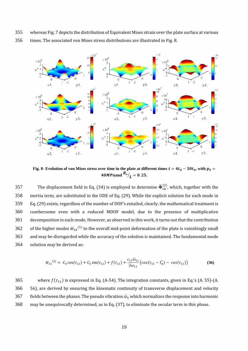
whereas Fig. 7 depicts the distribution of Equivalent Mises strain over the plate surface at various 355

times. The associated von Mises stress distributions are illustrated in Fig. 8. 356

Fig. 8- Evolution of von Mises stress over time in the plate at different times 𝒕 = 𝟒𝒕𝒅 − 𝟑𝟎𝒕𝒅, with 𝒑𝟎 =

𝟒𝟎𝑴𝑷𝒂and 𝑹𝒆

𝑳⁄ = 𝟎. 𝟐𝟓.

The displacement field in Eq. (34) is employed to determine �̅�1𝑘(2)

, which, together with the 357

inertia term, are substituted in the ODE of Eq. (29). While the explicit solution for each mode in 358

Eq. (29) exists, regardless of the number of DOF’s entailed, clearly, the mathematical treatment is 359

cumbersome even with a reduced MDOF model, due to the presence of multiplicative 360

decomposition in each mode. However, as observed in this work, it turns out that the contribution 361

of the higher modes �̅�33(1) to the overall mid-point deformation of the plate is vanishingly small 362

and may be disregarded while the accuracy of the solution is maintained. The fundamental mode 363

solution may be derived as: 364

�̅�11(2) = 𝐶4 cos(𝜏11) + 𝐶5 sin(𝜏11) + 𝑓(𝜏11) +

𝑐11�̅�11

2𝜔11

(𝑐𝑜𝑠(𝜏11 − 𝑡�̅�) − 𝑐𝑜𝑠(𝜏11)) (36)

where 𝑓(𝜏11) is expressed in Eq. (A-54). The integration constants, given in Eq.’s (A. 55)-(A. 365

56), are derived by ensuring the kinematic continuity of transverse displacement and velocity 366

fields between the phases. The pseudo vibration �̅�1 which normalizes the response into harmonic 367

may be unequivocally determined, as in Eq. (37), to eliminate the secular term in this phase. 368

20

�̅�11 = [0.8 − (0.29𝑠𝑖𝑛(𝑡�̅�)4 − 0.22𝑠𝑖𝑛(𝑡�̅�)

2 + 0.8)𝑐𝑜𝑠(𝑡�̅�)]𝐸𝑐11

2

𝐿2𝜌𝜔11 (37)

For an SDOF system, this parameter would reduce to: 369

�̅�1 =3𝐸𝑐11

2

4𝐿2𝜌𝜔11

(1 − 𝑐𝑜𝑠(𝑡�̅�)) (38)

A comparison of �̅�1′s for SDOF and MDOF model in Fig. 9 reveals an insignificant difference 370

between the two values indeed. In Fig. 10, the interaction between the load duration, central 371

constant load radius and �̅�1 is graphed for various values of thickness. 372

Fig. 9 Comparison of SDOF and MDOF pseudo vibrations

373

21

Fig. 10- Interaction surface of the load duration, Load

radius and pseudo vibration for SDOF model

Similarly, for the second mode �̅�13(2)

we have: 374

�̅�13(2) = 𝐶6 cos(𝜏11) + 𝐶7 sin(𝜏11) + 𝑓(𝜏13) +

𝑐13�̅�13

2𝜔13

(𝑐𝑜𝑠(𝜏13 − 𝑡�̅�) − 𝑐𝑜𝑠(𝜏13)) (39)

Where Eq. (A-57) gives the function 𝑓(𝜏13), while the integration constants are expressed in 375

Eq.’s (A. 58)-(A. 59). It should be stressed that in this phase �̅�13 ≅ �̅�11 applies. 376

Fig. 11 Variations of the pseudo vibrations with

vibration frequency

This concludes the two phases of motion and the method adopted is universally applicable. 377

22

4 Influence of pulse shape 378 379

It has been shown the pulse shape has a pronounced effect on the response of plates made of 380

rigid-perfectly plastic materials. It would be interesting to see if the influence of pulse shape on 381

FVK plate is significant. This effect is investigated on the plates studied here. More often than not, 382

a non-impulsive pressure load may assume various temporal pulse shapes contingent upon the 383

source of blast. A general expression of pulse shapes expressed by Li and Meng [3] reads: 384

𝑝2(𝑡) = {(1 − 𝑋

𝑡

𝑡𝑑) 𝑒

−𝑌𝑡𝑡𝑑, 0 ≤ 𝑡 ≤ 𝑡𝑑

0 𝑡𝑑 ≤ 𝑡

(40)

Fig. 12- Typical temporal pulse loading shapes (R) rectngular

(L) linear, (E) exponential

385

where X and Y are pulse shape parameters obtained experimentally or numerically. Through 386

the correct choice of these parameters, the expression in Eq. (40) can define any linear or 387

exponential pulse, while in the case of 𝑋 = 𝑌 = 0, Eq. (40) reduces to the case of a rectangular 388

pulse. The expression of �̅�𝑚𝑛(1)

would be modified in the first phase of motion as: 389

𝑤𝑚𝑛(1)

= 𝐶1𝑐𝑜𝑠(𝜔𝑚𝑛𝑡) + 𝐶2𝑠𝑖𝑛(𝜔𝑚𝑛𝑡)

+ −((𝑋𝑡 − 𝑡𝑑)(𝜔𝑚𝑛

2 𝑡𝑑2 + 𝑌2) + 2𝑋𝑌𝑡𝑑) 𝑡𝑑𝑐𝑚𝑛𝜔𝑚𝑛

2 𝑒−

𝑌𝑡𝑡𝑑

(𝜔𝑚𝑛2 𝑡𝑑

2 + 𝑌2)2

(41)

where the constants 𝐶1 and 𝐶2 are obtained as: 390

𝐶1 =(−𝜔𝑚𝑛

2 𝑡𝑑2 + 2𝑋𝑌 − 𝑌2)𝜔𝑚𝑛

2 𝑡𝑑2

(𝜔𝑚𝑛2 𝑡𝑑

2 + 𝑌2)2𝑐𝑚𝑛 (42)

23

𝐶2 = −𝑡𝑑𝑐𝑚𝑛𝜔𝑚𝑛(−𝑋𝜔11

2 𝑡𝑑2 − 𝑌𝜔𝑚𝑛

2 𝑡𝑑2 + 𝑋𝑌2 − 𝑌3)

(𝜔𝑚𝑛2 𝑡𝑑

2 + 𝑌2)2 (43)

Similarly, for the second phase of motion, 391

𝑤𝑚𝑛(1)

=𝑐𝑚𝑛𝜔𝑚𝑛𝑡𝑑

(𝜔𝑚𝑛2 𝑡𝑑

2 + 𝑌2)2(𝐺1𝑠𝑖𝑛(𝜔𝑚𝑛𝑡) + 𝐸1𝑐𝑜𝑠(𝜔𝑚𝑛𝑡)) (44)

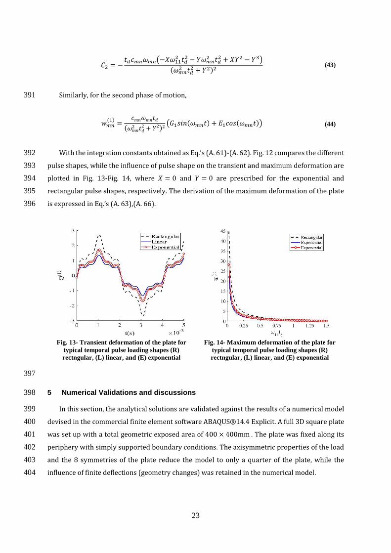
With the integration constants obtained as Eq.’s (A. 61)-(A. 62). Fig. 12 compares the different 392

pulse shapes, while the influence of pulse shape on the transient and maximum deformation are 393

plotted in Fig. 13-Fig. 14, where 𝑋 = 0 and 𝑌 = 0 are prescribed for the exponential and 394

rectangular pulse shapes, respectively. The derivation of the maximum deformation of the plate 395

is expressed in Eq.’s (A. 63),(A. 66). 396

Fig. 13- Transient deformation of the plate for

typical temporal pulse loading shapes (R)

rectngular, (L) linear, and (E) exponential

Fig. 14- Maximum deformation of the plate for

typical temporal pulse loading shapes (R)

rectngular, (L) linear, and (E) exponential

397

5 Numerical Validations and discussions 398

In this section, the analytical solutions are validated against the results of a numerical model 399

devised in the commercial finite element software ABAQUS®14.4 Explicit. A full 3D square plate 400

was set up with a total geometric exposed area of 400 × 400mm . The plate was fixed along its 401

periphery with simply supported boundary conditions. The axisymmetric properties of the load 402

and the 8 symmetries of the plate reduce the model to only a quarter of the plate, while the 403

influence of finite deflections (geometry changes) was retained in the numerical model. 404

24

The material properties were those of isotropic elastic metals with high yield strength such 405

as ARMOX 440T sheets. These panels were High Hardness Armour graded steel alloy types used 406

for blast protective plates and manufactured by SSAB® [39], [40]. The geometric and material 407

properties of the plates were taken from [8] (Table 1). 408

The models were discretized with a fine mesh of four-noded S4R isoparametric general shell 409

elements with reduced integration and finite membrane strains possessing 5 Simpson integration 410

points through the thickness of the plate. These elements are general-purpose conventional shells 411

with the reduced integration formulation and hourglass control to prevent both shear locking and 412

spurious energy (hour glassing). A total of 2500 elements were assigned to give the quotient of 413

the element length to thickness as 0.87 to satisfy the convergence [8]. 414

Two blast loading scenarios of 40MPa and 200MPa magnitudes were assumed, with pulse 415

shape of rectangular profile and duration of 100𝜇𝑠 and 30𝜇𝑠, respectively. The radius of the 416

central uniform blast zone was taken to be 25mm and 50mm for each case, respectively. The 417

transient deformation of the panels was investigated in each blast scenario the results of which 418

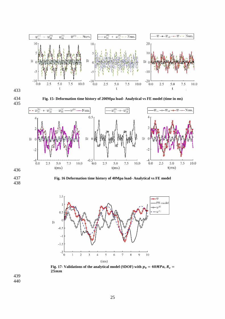
are shown in Fig. 15 and Fig. 16. Fig. 17 also compares the transient deformation for the SDOF 419

model with a blast load of amplitude 40𝑀𝑃𝑎 and 50𝜇𝑠 loading duration with the numerical 420

model. 421

Clearly, while the vibration frequency of the analytical model in its first (fundamental mode) 422

is lower than its FE counterpart, in the higher modes the frequencies increase while the peak 423

displacements decrease. The higher modes enhance the residual vibrations at each cycle but 424

infinitesimally affect the overall peak deformation. For example, like the first phase, the peak 425

deformation of the first mode was found to be 70% higher than the second mode. Furthermore, 426

there is a good agreement between the analytical and numerical models in prediction of peak 427

displacements. Consequently, the mathematical treatment of the problem favoring only the first 428

and second modes would suffice to predict the response. 429

In Table 2 and Table 3 the peak deformation from the numerical models and the analytical 430

counterparts for various blast load radii compare favourably. Higher errors are attributed to 431

more uniform blasts which may be due to overprediction of the load parameter. 432

25

433

Fig. 15- Deformation time history of 200Mpa load- Analytical vs FE model (time in ms) 434 435

436

Fig. 16 Deformation time history of 40Mpa load- Analytical vs FE model 437 438

Fig. 17- Validations of the analytical model (SDOF) with 𝒑𝟎 = 𝟒𝟎𝑴𝑷𝒂, 𝑹𝒆 =𝟐𝟓𝒎𝒎

439

440

26

Table 2 Peak central displacement of the plate on 𝒑𝟎 = 𝟒𝟎𝑴𝑷𝒂, analytical vs FE model 441

𝑅𝑒/𝐿 �̅�11 �̅�13 �̅�33 �̅� ABAQUS % Error

0.125 1.46 0.28 0.13 2.15 2.63 18.37

0.25 2.82 0.53 0.26 4.14 3.94 5.04

0.375 4.09 0.77 0.37 6.01 5.17 16.10

0.5 4.91 0.93 0.45 7.21 6.25 15.36

442

443 Table 3- Peak central displacement of the plate on 𝒑𝟎 = 𝟐𝟎𝟎𝑴𝑷𝒂, analytical vs FE model 444

𝑅𝑒/𝐿 �̅�11 �̅�13 �̅�33 �̅� ABAQUS % Error

0.125 2.20 0.44 0.24 2.88 3.21 10.27

0.25 4.24 0.84 0.46 5.55 4.78 16.14

0.375 6.15 1.22 0.67 8.05 6.36 26.60

0.5 7.38 1.47 0.81 9.66 7.52 28.46

445

6 Concluding remarks 446 447

This work deals with dynamic response of nonlinear elastic thin plated structures subject to 448

localised blasts due to proximal charges. The localised blast load was assumed to be 449

multiplicatively decomposable into a spatial and a temporal distribution. Considering this 450

idealization, and using the Ritz-Galerkin functional, a single dimensionless parameter was 451

obtained which characterises various blast loading scenarios by the correct choice of its 452

parameters 𝑏, 𝑅𝑒 . 453

The Ritz-Galerkin method was similarly employed to minimize the nonlinear coupled FVK 454

equations considering a kinematically admissible displacement field and an associated Airy stress 455

function as a truncated cosine series - each term representative of a unique mode of vibration- in 456

an iterative procedure. The state variables were determined in two distinguished phases of 457

motion, the first reflecting the forced vibration while the second addressing the free vibration due 458

to initial inertia effects and the stored elastic energy of the system. The Poincaré-Lindstedt 459

perturbation method was employed to avoid the non-convergent explicit solution due to the 460

presence of secular terms whilst satisfying a predicted harmonic oscillation. 461

The presence of higher modes had little effect on the overall response of the plate as the 462

observed peak deformations from the first to second mode decreased significantly and were more 463

diminutive with respect to the fourth mode (�̅�33). The MDOF model offered more accurate 464

oscillation frequency, capable of predicting the residual vibrations. The results of dynamic 465

analyses conducted were corroborated with the commercial FE software ABAQUS/Explicit and 466

strong correlation was observed in all cases. 467

27

The influence of pulse shape was investigated whereby significant differences between the 468

impulsive-characterised pulse and rectangular pulse- and non-impulsive blasts were observed. 469

In accordance with the results of [23], clearly, the blast load is in a state of attenuation with the 470

increase of the load temporal decay parameter (Y), leading to the decrease of response 471

amplitudes. Similar trend is evident with the variation of the load shape decay parameter (b). 472

473

7 Citations 474 [1] D. Bonorchis and G. N. Nurick, “The influence of boundary conditions on the loading of rectangular plates 475

subjected to localised blast loading - Importance in numerical simulations,” Int. J. Impact Eng., vol. 36, no. 1, pp. 476 40–52, 2009. 477

[2] N. Mehreganian, A. S Fallah, and L. A. Louca, “Inelastic dynamic response of square membranes subjected to 478 localised blast loading,” Int. J. Mech. Sci., vol. 148, no. August, pp. 578–595, 2018. 479

[3] Q. M. Li and H. Meng, “Pulse loading shape effects on pressure-impulse diagram of an elastic-plastic, single-480 degree-of-freedom structural model,” Int. J. Mech. Sci., vol. 44, no. 9, pp. 1985–1998, 2002. 481

[4] A. S. Fallah and L. A. Louca, “Pressure-impulse diagrams for elastic-plastic-hardening and softening single-degree-482 of-freedom models subjected to blast loading,” Int. J. Impact Eng., vol. 34, no. 4, pp. 823–842, 2007. 483

[5] C. Zheng, X. S. Kong, W. G. Wu, and F. Liu, “The elastic-plastic dynamic response of stiffened plates under 484 confined blast load,” Int. J. Impact Eng., vol. 95, pp. 141–153, 2016. 485

[6] P. S. Symonds, “Elastic, Finite Deflection and Strain Rate Effects in a Mode Approximation Technique for Plastic 486 Deformation of Pulse Loaded Structures.,” J. Mech. Eng. Sci., vol. 22, no. 4, pp. 189–197, 1980. 487

[7] N. Jones, Structural Impact, 1st ed. Cambridge: Cambridge University Press, 1997. 488 [8] N. Mehreganian, L. A. Louca, G. S. Langdon, R. J. Curry, and N. Abdul-Karim, “The response of mild steel and 489

armour steel plates to localised air-blast loading-comparison of numerical modelling techniques,” Int. J. Impact 490 Eng., vol. 115, no. January, pp. 81–93, 2018. 491

[9] B. McDonald, H. Bornstein, G. S. Langdon, R. Curry, A. Daliri, and A. C. Orifici, “Experimental response of high 492 strength steels to localised blast loading,” Int. J. Impact Eng., vol. 115, no. October 2017, pp. 106–119, 2018. 493

[10] P. S. Symonds and W. T. Fleming, “Parkes revisited: On rigid-plastic and elastic-plastic dynamic structural 494 analysis,” Int. J. Impact Eng., vol. 2, no. 1, pp. 1–36, 1984. 495

[11] S. Vidoli, “Discrete approximations of the Föppl – Von Kármán shell model : From coarse to more refined models,” 496 Int. J. Solids Struct., vol. 50, no. 9, pp. 1241–1252, 2013. 497

[12] E. H. DOWELL and C. S. VENTRES, “Comparison of theory and experiment for nonlinear flutter of loaded 498 plates,” AIAA J., vol. 8, no. 11, pp. 2022–2030, 1970. 499

[13] E. H. . Dowell and O. Bendiksen, Panel flutter. Encyclopedia of Aerospace Engineering. John Wiley & Sons, 2010. 500 [14] P. Del Linz, X. Liang, P. A. Hooper, L. Z. Wang, and J. P. Dear, “An analytical solution for pre-crack behaviour of 501

laminated glass under blast loading,” Compos. Struct., vol. 144, pp. 156–164, 2016. 502 [15] Y. Yuan, P. J. Tan, and Y. Li, “Dynamic structural response of laminated glass panels to blast loading,” Compos. 503

Struct., vol. 182, no. August, pp. 579–589, 2017. 504 [16] P. Hooper, “Blast performance of silicone-bonded laminated glass (PhD Thesis),” Imperial College London, 2011. 505 [17] M. L. Dano and M. W. Hyer, “Thermally-induced deformation behavior of unsymmetric laminates,” Int. J. Solids 506

Struct., vol. 35, no. 17, pp. 2101–2120, 1998. 507 [18] J. Dervaux, P. Ciarletta, and M. Ben Amar, “Morphogenesis of thin hyperelastic plates: A constitutive theory of 508

biological growth in the Föppl-von Kármán limit,” J. Mech. Phys. Solids, vol. 57, no. 3, pp. 458–471, 2009. 509 [19] T.-L. Teng, C.-C. Liang, and Liao-Ching-Cho, “Transient Dynamic Large-Deflection Analysis of Panel Structure 510

under Blast Loading,” Japan Soc. Mech. Eng., vol. 339, no. 4, pp. 591–597, 1996. 511 [20] V. R. Feldgun, D. Z. Yankelevsky, and Y. S. Karinski, “A nonlinear SDOF model for blast response simulation of 512

elastic thin rectangular plates,” Int. J. Impact Eng., vol. 88, pp. 172–188, 2016. 513 [21] G. Chandrasekharappa and H. R. Srirangarajan, “Nonlinear response of elastic plates to pulse excitations,” Comput. 514

Struct., vol. 27, no. 3, pp. 373–378, 1987. 515 [22] T. Liu, W. Zhang, and J. . Wang, “Nonlinear dynamics of composite laminated circular cylindrical shell clamped 516

along a generatrix and with membranes at both ends,” Nonlinear Dyn., vol. 90, no. 2, pp. 1393–1417, 2017. 517 [23] A. Wang, H. Chen, and W. Zhang, “Nonlinear transient response of doubly curved shallow shells reinforced with 518

graphene nanoplatelets subjected to blast loads considering thermal effects,” Compos. Struct., vol. 225, no. May, p. 519 111063, 2019. 520

[24] J. . Reddy, Mechanics of Laminated Composite Plates and Shells: Theory and Analysis, 2nd ed. London: CRC 521 Press, 2004. 522

[25] W. Zhang, T. Liu, A. Xi, and Y. N. Wang, “Resonant responses and chaotic dynamics of composite laminated 523 circular cylindrical shell with membranes,” J. Sound Vib., vol. 423, no. March, pp. 65–99, 2018. 524

[26] W. Zhang, J. Yang, and Y. Hao, “Chaotic vibrations of an orthotropic FGM rectangular plate based on third-order 525 shear deformation theory,” Nonlinear Dyn., vol. 59, pp. 619–660, 2010. 526

28

[27] N. Jacob, G. N. Nurick, and G. S. Langdon, “The effect of stand-off distance on the failure of fully clamped circular 527 mild steel plates subjected to blast loads,” Eng. Struct., vol. 29, no. 10, pp. 2723–2736, 2007. 528

[28] C. N. Kingery and N. Bulmash, “Air blast parameters from TNT spherical air burst and hemispherical surface burst, 529 Report ARBL-TR-02555,” MD, 1984. 530

[29] V. Aune, G. Valsamos, F. Casadei, M. Larcher, M. Langseth, and T. Børvik, “Numerical study on the structural 531 response of blast-loaded thin aluminium and steel plates,” Int. J. Impact Eng., vol. 99, pp. 131–144, 2017. 532

[30] D. Karagiozova, G. S. Langdon, G. N. Nurick, and S. Chung Kim Yuen, “Simulation of the response of fibre-metal 533 laminates to localised blast loading,” Int. J. Impact Eng., vol. 37, no. 6, pp. 766–782, 2010. 534

[31] A. S. Fallah, K. Micallef, G. S. Langdon, W. C. Lee, P. T. Curtis, and L. A. Louca, “Dynamic response of 535 Dyneema® HB26 plates to localised blast loading,” Int. J. Impact Eng., vol. 73, no. November, pp. 91–100, 2014. 536

[32] K. Micallef, A. S. Fallah, D. J. Pope, and L. A. Louca, “The dynamic performance of simply-supported rigid-plastic 537 circular steel plates subjected to localised blast loading,” Int. J. Mech. Sci., vol. 65, no. 1, pp. 177–191, 2012. 538

[33] G. K. Schleyer, S. S. Hsu, M. D. White, and R. S. Birch, “Pulse pressure loading of clamped mild steel plates,” Int. 539 J. Impact Eng., vol. 28, no. 2, pp. 223–247, 2003. 540

[34] V. Aune, E. Fagerholt, K. O. Hauge, M. Langseth, and T. Børvik, “Experimental study on the response of thin 541 aluminium and steel plates subjected to airblast loading,” Int. J. Impact Eng., vol. 90, pp. 106–121, 2016. 542

[35] C. K. Youngdahl, “Correlation parameters for eliminating the effects of pulse shape on dynamic plate deformation,” 543 Trans. ASME J. Appl. Mech., vol. 37, no. 2, pp. 744–752, 1970. 544

[36] Q. M. Li and N. Jones, “Foundation of Correlation Parameters for Eliminating Pulse Shape Effects on Dynamic 545 Plastic Response of Structures,” J. Appl. Mech., vol. 72, no. 2, p. 172, 2005. 546

[37] Y. Yuan, P. J. Tan, K. A. Shojaei, and P. Wrobel, “Large deformation, damage evolution and failure of ductile 547 structures to pulse-pressure loading,” Int. J. Solids Struct., vol. 96, pp. 320–339, 2016. 548

[38] A. H. Nayfeh, Introduction to Perturbation Techniques, vol. 20. New York: Wiley-Interscience Publication, 1993. 549 [39] SSAB, “Armox Blast Protection Plate,” SSAB Swedish Steel Ltd, 2018. . 550 [40] T. Cwik and B. Se, “Project report : Ballistic performance of Armox 370T and Armox 440 steels,” no. June, 2015. 551

552 553

Appendix A 554

A1. Stress tensor components and stiffness matrices 555

The significant (non-zero) components of the stress tensor (with 𝑖 ≥ 1) may be expressed as: 556

𝜎22(𝑖+1)

=𝜋2

𝐿2𝐸𝐻2 [−

1

4Φ̅11

(i+1) 𝑐𝑜𝑠 (

𝜋𝑥

2𝐿) 𝑐𝑜𝑠 (

𝜋𝑦

2𝐿) −

9

4Φ̅13

(i+1)𝑐𝑜𝑠 (

3𝜋𝑥

2𝐿) 𝑐𝑜𝑠 (

𝜋𝑦

2𝐿)

−1

4Φ̅13

(i+1)𝑐𝑜𝑠 (

𝜋𝑥

2𝐿) 𝑐𝑜𝑠 (

3𝜋𝑦

2𝐿) −

9

4Φ̅33

(i+1)𝑐𝑜𝑠 (

3𝜋𝑥

2𝐿) 𝑐𝑜𝑠 (

3𝜋𝑦

2𝐿)]

(A. 45)

𝜎11(𝑖+1)

=𝜋2

𝐿2𝐸𝐻2 [−

1

4Φ̅11

(i+1) 𝑐𝑜𝑠 (

𝜋𝑥

2𝐿) 𝑐𝑜𝑠 (

𝜋𝑦

2𝐿) −

9

4Φ̅13

(i+1)𝑐𝑜𝑠 (

𝜋𝑥

2𝐿) 𝑐𝑜𝑠 (

3𝜋𝑦

2𝐿)

−1

4Φ̅13

(i+1)𝑐𝑜𝑠 (

3𝜋𝑥

2𝐿) 𝑐𝑜𝑠 (

𝜋𝑦

2𝐿) −

9

4Φ̅33

(i+1)𝑐𝑜𝑠 (

3𝜋𝑥

2𝐿) 𝑐𝑜𝑠 (

3𝜋𝑦

2𝐿)]

(A. 46)

𝜎12(𝑖+1)

=𝜋2

𝐿2𝐸𝐻2 [

1

4Φ̅11

(i+1) 𝑠𝑖𝑛 (

𝜋𝑥

2𝐿) 𝑠𝑖𝑛 (

𝜋𝑦

2𝐿) +

3

4Φ̅13

(i+1)𝑠𝑖𝑛 (

3𝜋𝑥

2𝐿) 𝑠𝑖𝑛 (

𝜋𝑦

2𝐿)

+3

4Φ̅13

(i+1)𝑠𝑖𝑛 (

𝜋𝑥

2𝐿) 𝑠𝑖𝑛 (

3𝜋𝑦

2𝐿) +

9

4Φ̅33

(i+1)𝑠𝑖𝑛 (

3𝜋𝑥

2𝐿) 𝑠𝑖𝑛 (

3𝜋𝑦

2𝐿)]

(A. 47)

The coefficients of the matrix 𝑩𝑚𝑛 are given as: 557

29

𝐵11 =

[ −

2

3−

22

45−

22

45

2

5

−22

45−

114

35−

166

225−

162

175

−22

45−

166

225−

114

35−

162

175

2

5−

162

175−

162

175−

162

35 ]

(A-48)

𝐵13 =

[ −

22

45−

166

225−

114

35−

162

175

−166

225−

186

35−

186

35−

26406

1225

−114

35−

166

2252 −

22

15

−162

175−

26406

1225−

22

15

342

35 ]

(A-49)

𝐵33 =

[

2

5 −

162

175−

162

175−

162

35

−162

175

22

15−

26406

1225

342

35

−162

175−

26406

1225

22

15

342

35

−162

35

342

35

342

35−6 ]

(A-50)

558

The components of Airy Stress function are expressed as: 559

�̅�11(i+1)

= −4

𝜋2{1

3�̅�11

(𝑖)2 +44

45�̅�11

(𝑖)�̅�13(𝑖) + −

2

5�̅�11

(𝑖)�̅�33(𝑖) +

6292

1575�̅�13

(𝑖)2 +324

175�̅�13

(𝑖)�̅�33(𝑖) +

81

35�̅�33

(𝑖)2} (A. 51)

560

�̅�13(𝑖+1)

= −4

275625𝜋2{2695�̅�11

(𝑖)2 + 44044�̅�11(𝑖)�̅�13

(𝑖) + 10206�̅�11(𝑖)�̅�33

(𝑖) + 76860�̅�13(𝑖)2

+ 221484�̅�13(𝑖)�̅�33

(𝑖) − 53865�̅�33(𝑖)2}

(A. 52)

561

�̅�33(𝑖+1)

= −4

297675𝜋2{735�̅�11

(𝑖)2 − 6804�̅�11(𝑖)�̅�13

(𝑖) − 170106�̅�11(𝑖)�̅�33

(𝑖) − 73828�̅�13(𝑖)2

+ 71820�̅�13(1)

�̅�33(1)

− 11025�̅�33(1)2

}

(A. 53)

30

and �̅�𝑖𝑗(𝑖)

= �̅�𝑗𝑖(i) as the Airy Stress function exhibits symmetry. 562

A2. Second phase of motion parameters 563

Regarding the first mode of the displacement field at second phase of motion we have: 564

𝑓(𝜏11) ≅ −𝐸𝑐11

3

𝐿2𝜔112 𝜌

(0.0395(𝑐𝑜𝑠(3𝜏11) − 𝑐𝑜𝑠(3𝜏11 − 3𝑡�̅�))

+ 0.098(𝑐𝑜𝑠(3𝜏11 − 2𝑡�̅�) − 𝑐𝑜𝑠(3𝜏11 − 𝑡�̅�))

+ 0.0134(𝑐𝑜𝑠(3𝜏11 − 4𝑡�̅�) − 𝑐𝑜𝑠(3𝜏11 + 𝑡�̅�))

+ 0.598(𝑐𝑜𝑠(𝜏11 − 𝑡�̅�) − 𝑐𝑜𝑠(𝜏11))

+ 0.196(𝑐𝑜𝑠(𝜏11 + 𝑡�̅�) − 𝑐𝑜𝑠(𝜏11 − 2𝑡�̅�)))

(A-54)

Where the integration constants 565

𝐶4 =𝑐11

3 𝐸

𝐿2𝜌𝜔112 (−1.6𝑐𝑜𝑠(𝑡�̅�) + 2.0753 − 0.269𝑐𝑜𝑠(2𝑡�̅�) − 0.192𝑐𝑜𝑠(3𝑡�̅�))

+𝑐11�̅�11

2𝜔11

(1 − 𝑐𝑜𝑠(𝑡�̅�))

(A. 55)

566

𝐶5 ≅𝐸𝑐11

3

𝜌𝐿2𝜔112 (−0.27𝑠𝑖𝑛(2𝑡�̅�) + −0.1946𝑠𝑖𝑛(3𝑡�̅�) − 0.0015𝑠𝑖𝑛(7𝑡�̅�) − 3.2940𝑠𝑖𝑛(𝑡�̅�))

−𝑐11�̅�11

2𝜔11

𝑠𝑖𝑛(𝑡�̅�)

(A. 56)

Similarly, for the higher modes: 567

𝑓(𝜏13) ≅𝑐13

3 𝐸

𝜔132 𝜌 𝐿2

(−5616𝑐𝑜𝑠(0.6𝜏13 + 0.2𝑡�̅�) − 16460𝑐𝑜𝑠(0.6𝜏13 − 0.2𝑡�̅�)

− 3744𝑐𝑜𝑠(1.4𝜏13 − 1.2𝑡�̅�) − 34080𝑐𝑜𝑠(0.2(𝜏13 − 𝑡�̅�))

− 2808𝑐𝑜𝑠(0.6𝜏13 − 𝑡�̅�) + 3744𝑐𝑜𝑠(1.4𝜏13 − 0.2𝑡�̅�)+ +5616𝑐𝑜𝑠(0.6𝜏13 − .8𝑡�̅�) + 8294𝑐𝑜𝑠(0.6𝜏13)

− 10970 cos(0.2(𝜏13 + 𝑡�̅�)) + 2808𝑐𝑜𝑠(0.6𝜏13 + 0.4𝑡�̅�)

− 8294𝑐𝑜𝑠(0.6𝜏13 − 0.6𝑡�̅�) + 16460𝑐𝑜𝑠(0.6𝜏13 − 0.4𝑡�̅�)

+ 10970𝑐𝑜𝑠(. 2𝜏13 − .4𝑡�̅�) + 34080𝑐𝑜𝑠(0.2𝜏13))

+�̅�13

2𝜔13

𝑐13(𝑐𝑜𝑠(𝜏13 − 𝑡𝑑𝑏𝑎𝑟) − 𝑐𝑜𝑠(𝜏13))

(A-57)

𝐶6 ≅𝑐13�̅�13

2𝜔13

(1 − 𝑐𝑜𝑠(𝑡�̅�)) −𝐸𝑐13

3

𝐿2𝜔132 𝜌

(1733𝑐𝑜𝑠(2𝑡�̅�) + 566.3𝑐𝑜𝑠(2.2𝑡�̅�) + 2485𝑐𝑜𝑠(0.6𝑡�̅�)

+ 1465𝑐𝑜𝑠(1.2𝑡�̅�) − 1493𝑐𝑜𝑠(1.4𝑡�̅�) − 1797𝑐𝑜𝑠(0.2𝑡�̅�)

+ −6609𝑐𝑜𝑠(.8𝑡�̅�) + 43.52𝑐𝑜𝑠(3.2𝑡�̅�) + 426.7𝑐𝑜𝑠(1.8𝑡�̅�) + 4217𝑐𝑜𝑠(𝑡�̅�)

− 1012)

(A. 58)

568

31

𝐶7 = −𝑐13�̅�13

2𝜔13

𝑠𝑖𝑛(𝑡�̅�) −𝐸𝑐13

3

𝐿2𝜔132 𝜌

(1733𝑠𝑖𝑛(2𝑡�̅�) + 566.3𝑠𝑖𝑛(2.2𝑡�̅�) + 2485𝑠𝑖𝑛(.6𝑡�̅�)

+ 1697𝑠𝑖𝑛(1.2𝑡�̅�) − 1493𝑠𝑖𝑛(1.4𝑡�̅�) + 49.72𝑠𝑖𝑛(2.8𝑡�̅�) − 75.78𝑠𝑖𝑛(3𝑡�̅�)

+ 27199𝑠𝑖𝑛(0.2𝑡�̅�) − 6261𝑠𝑖𝑛(0.8𝑡�̅�) + 43.52𝑠𝑖𝑛(3.2𝑡�̅�)

+ 426.7𝑠𝑖𝑛(1.8𝑡�̅�) + 3805𝑠𝑖𝑛(𝑡�̅�)

(A. 59)

Full expression of �̅�33(1)

is given as: 569

�̅�33(1)

= −𝑐11

3 𝐸

𝐿2𝜔332 𝜌

(0.106𝑐𝑜𝑠(𝜏33) − 0.882 + 3.79 × 10−4𝑐𝑜𝑠(2𝜏33) + 0.105𝑐𝑜𝑠 (10

3𝜏33)

+ 1.48𝑐𝑜𝑠 (10

9𝜏33) + 3.28 × 10−4𝑐𝑜𝑠(1.44𝜏33) + 8.05 × 10−4𝑐𝑜𝑠 (

5

3𝜏33)

− 2.24 × 10−4𝑐𝑜𝑠 (17

9𝜏33) + 0.0799𝑐𝑜𝑠 (

11

9𝜏33) + 1.87 × 10−4𝑐𝑜𝑠 (

19

9𝜏33)

− 0.186𝑐𝑜𝑠 (7

9𝜏33) + 0.449𝑐𝑜𝑠 (

2

3𝜏33) − 0.741𝑐𝑜𝑠 (

2

9𝜏33) − 0.619𝑐𝑜𝑠 (

5

9𝜏33)

− 3.81 × 10−3𝑐𝑜𝑠 (14

9𝜏33) − 0.583𝑐𝑜𝑠 (

10

9𝜏33) + 0.477𝑐𝑜𝑠 (

8

9𝜏33)

+ 0.318𝑐𝑜𝑠 (4

9𝜏33))

(A-60)

A3. Dynamic pulse pressure loading 570

The integration constants of the displacement field considering the influence of pulse shape 571

are: 572

𝐺1 = {(𝜔𝑚𝑛2 𝑡𝑑

2((𝑋 − 1)𝑌 − 𝑋) + 𝑌2((𝑋 − 1)𝑌 + 𝑋)) 𝑐𝑜𝑠(𝜔𝑚𝑛𝑡𝑑)

− 𝜔𝑚𝑛𝑡𝑑𝑠𝑖𝑛(𝜔𝑚𝑛𝑡𝑑) (𝜔𝑚𝑛2 𝑡𝑑

2(𝑋 − 1) + 𝑌((𝑋 − 1)𝑌 + 2𝑋))} 𝑒−𝑌

+ 𝑡𝑑2𝜔𝑚𝑛

2 (𝑋 + 𝑌) − 𝑌2(𝑋 − 𝑌)

(A. 61)

𝐸1 = − ({(𝑡𝑑2((𝑋 − 1)𝑌 − 𝑋)𝜔𝑚𝑛

2 + 𝑌2((𝑋 − 1)𝑌 + 𝑋)) 𝑠𝑖𝑛(𝜔𝑚𝑛𝑡𝑑)

+ (𝑡𝑑2𝜔𝑚𝑛

2 (𝑋 − 1) + 𝑌((𝑋 − 1)𝑌 + 2𝑋)) 𝑐𝑜𝑠(𝜔𝑚𝑛𝑡𝑑)𝜔𝑚𝑛𝑡𝑑} 𝑒−𝑌 + 𝜔𝑚𝑛3 𝑡𝑑

3

+ 𝑌2 − 2𝑋𝑌𝜔𝑚𝑛𝑡𝑑)

(A. 62)

For a linear pulse shape, 𝑌 = 0, Eq. (44) is reduced to: 573

𝑤𝑚𝑛(1)

= −𝑐𝑚𝑛

𝜔𝑚𝑛𝑡𝑑(𝐺2𝑠𝑖𝑛(𝜔𝑚𝑛𝑡) + 𝐸2𝑐𝑜𝑠(𝜔𝑚𝑛𝑡)) (A. 63)

𝐺2 = (𝑋(𝑐𝑜𝑠(𝜔𝑚𝑛𝑡𝑑) − 1) + 𝜔𝑚𝑛𝑡𝑑(𝑋 − 1)𝑠𝑖𝑛(𝜔𝑚𝑛𝑡𝑑)) (A. 64)

𝐸2 = (𝜔𝑚𝑛𝑡𝑑(𝑋 − 1)𝑐𝑜𝑠(𝜔𝑚𝑛𝑡𝑑) − 𝑋𝑠𝑖𝑛(𝜔𝑚𝑛𝑡𝑑) + 𝜔𝑚𝑛𝑡𝑑) (A. 65)

32

Carrying out some algebraic manipulation, the deformation of the plate for a linear pulse 574

shape is expressed as 575

𝑤𝑚𝑛(1)

= −𝑾𝟐𝑠𝑖𝑛(𝜔𝑚𝑛𝑡 + 𝛽2)

(A. 66)

𝑾𝟐 =𝑐𝑚𝑛

𝜔𝑚𝑛𝑡𝑑√𝐸2

2 + 𝐺22 , 𝛽2 = tan−1 𝐸2/𝐺2 (A. 67)

In the same fashion, Eq. (44) may be recast in the form of 𝑾𝟑𝑠𝑖𝑛(𝜔𝑚𝑛𝑡 + 𝛽3) where the 576

maximum deformation of exponentially attenuating pulse is expressed as 577

𝑾𝟑 =𝑐𝑚𝑛𝜔𝑚𝑛𝑡𝑑

(𝜔𝑚𝑛2 𝑡𝑑

2 + 𝑌2)2√𝐸3

2 + 𝐺32 , 𝛽3 = tan−1 𝐸2/𝐺2 (A. 68)

𝐺3 = ((−𝑌𝜔𝑚𝑛2 𝑡𝑑

2 − 𝑌3)𝑐𝑜𝑠(𝜔𝑚𝑛𝑡𝑑) − 𝜔𝑚𝑛𝑡𝑑𝑠𝑖𝑛(𝜔𝑚𝑛𝑡𝑑)(−𝜔𝑚𝑛2 𝑡𝑑

2 − 𝑌2))𝑒−𝑌 + 𝑌𝜔𝑚𝑛2 𝑡𝑑

2

+ 𝑌3 (A. 69)

𝐸3 = (𝜔𝑚𝑛2 𝑡𝑑

2 + 𝑌2)((𝜔𝑚𝑛𝑡𝑑𝑐𝑜𝑠(𝜔𝑚𝑛𝑡𝑑) + 𝑠𝑖𝑛(𝜔𝑚𝑛𝑡𝑑)𝑌)𝑒−𝑌 − 𝜔𝑚𝑛𝑡𝑑) (A. 70)

578

579

580