Róbert Vrábeľ Nonlinear Dynamical Systems with High-Speed Feedback

Scientific Monographs in Automation and Computer Science Edited by Prof. Dr. Peter Husar (Ilmenau University of Technology) and Dr. Kvetoslava Resetova (Slovak University of Technology in Bratislava) Vol. 4

NONLINEAR DYNAMICAL SYSTEMS WITH HIGH-SPEED FEEDBACK

Róbert Vrábeľ

Universitätsverlag Ilmenau 2012

Impressum Bibliographic information of the German National Library The German National Library lists this publication in the German national bibliography, with detailed bibliographic information on the Internet at http://dnb.d-nb.de. Author’s acknowledgement to Dagmar Rusková for translation.

This scientific monograph originated from the author's habilitation thesis defended at the Slovak University of Technology in Bratislava, Faculty of Materials Science and Technology in Trnava. Reviewers:

Dušan Krokavec, Professor, Ph.D Dušan Mudrončík, Professor, Ph.D. Juraj Spalek, Professor, Ph.D.

Author’s contact address:

Róbert Vrábeľ, Assoc. Professor, Ph.D. Slovak University of Technology in Bratislava Faculty of Materials Science and Technology in Trnava

Ilmenau Technical University / University Library Universitätsverlag Ilmenau Postfach 10 05 65 98684 Ilmenau www.tu-ilmenau.de/universitaetsverlag Production and delivery Verlagshaus Monsenstein und Vannerdat OHG Am Hawerkamp 31 48155 Münster www.mv-verlag.de ISSN 2193-6439 (Print) ISBN 978-3-86360-016-7 (Print) URN urn:nbn:de:gbv:ilm1-2012100043 Titelfoto: photocase.com

Abstract

The aim of the work is to contribute to the qualitative and quan-

titative analysis of nonlinear dynamical systems of the second order

with high-speed feedback, which can also be generally introduced into

higher order systems which at present are gaining an increasing amount

of popularity in use of the high-frequency oscillators in electronic cir-

cuits. Singular Perturbation Theory is the mathematical framework

that yields the tools to explore the complicated dynamical behavior of

these systems. The work gives an overview of some methods used to

investigate the dynamics of singularly perturbed nonlinear systems, for

which does not exist a comprehensive theory that would give us an

overall view of their behavior.

This issue is currently happening world wide, not only in the math-

ematical community when dealing with the theory and application of

nonlinear dynamical systems, but also in the field of electrical engi-

neering and automation (contributions in research seminars and con-

ferences in the Centre for Intelligent Control, National University of

Singapore, IFAC Workshop on Singular Solutions and Perturbations

in Control Systems, Russia, 1997; IEEE Conference Decision and Con-

trol, New Orleans, USA, 2007; The 2009 IEEE International Conference

on Networking, Sensing and Control, Okayama University, Okayama,

Japan;. . . ).

Key words

nonlinear dynamical system of the second order with high-speed feed-

back, singularly perturbed nonlinear system, boundary layer

5

MOTIVATION AND INTRODUCTION

The work deals with the continuous nonlinear dynamical systems

with high-speed feedback which can be described by differential equa-

tions of the second order

ǫy′′ = f (t, y, y′, ǫ) (∗)

with a small parameter ǫ > 0 at the highest derivative and a continuous

function f . After rewriting into the system of differential equations

y′1 = y2

ǫy′2 = f (t, y1, y2, ǫ)

we are given a system of two differential equations of the first order.

This system we can reformulate as follows

y1 = ǫy2

y2 = f (ǫτ, y1, y2, ǫ) ,

where ˙= ddτand t = ǫτ. Both scalings agree on the level of the structure

of phase space system for ǫ 6= 0 but they are completely different in

the limit when ǫ → 0+. It is important to realize that τ → ∞ for

ǫ → 0+, which means that the small time interval for t (slow time)

corresponds to a large time interval for τ (fast time) which goes to

infinity asymptotically. When examining global properties of systems

described by a system of differential equations with a small parameter at

the highest derivative, this often uses a combination of both approaches

([3], [4]).

Naming such systems as dynamical systems with high-speed feed-

back follows due to the fact that for ǫ → 0+, with a finite right hand

6

side of a mathematical model in the expression ǫy′2 is allowed |y′2| → ∞at any point of the time interval. This situation is typical for many

cases interested in practice (Appendices A and B) in connection with

the phenomena arising in nonlinear systems such as auto-oscillations,

resonance, hysteresis, oscillations with large frequencies, . . . ([10], [14]).

Differential equations (systems) with a small parameter at the high-

est derivative in professional literature depicts as a singularly perturbed

system respecting the non validity of theorem about continuous depen-

dence of solutions on a parameter and resulting problems in the approx-

imation of solutions of differential equations in the right neighborhood

of ǫ = 0. The subject of exploration is the asymptotic behavior of these

systems, when the value of the parameter ǫ is close to zero.

In the 1st chapter we refer to inappropriateness of the use of ap-

proximate methods for nonlinear dynamical systems with high-speed

feedback and motivation to other parts of the work, where the used

methods of the theory of dynamical systems are suitable for the study

of nonlinear systems with high-speed feedback and especially those that

allow high-frequency oscillations.

The 2nd chapter summarizes the methods used in other parts of

the work and in Subsection 2.2.1 we describe the basic types of auto-

oscillations which may occur in autonomous systems of the 2nd order.

Appendices A and B are devoted to the existence and analysis of

high-frequency oscillations of nonlinear systems, namely for singular

perturbed oscillators of Duffing’s type. The systems considered here

constitute a structural mathematical model to describe and simulate

the nonlinear high-frequency circuits. For a review and for further ref-

erences, we refer to the article of Ping Mei, Chenxiao Cai, Yun Zou:

A Generalized KYP Lemma Based Approach for H∞ control of Singu-

7

larly Perturbed Systems published in the journal Circuits, Systems, and

Signal Processing, 2009, where the autonomous linear system

x′1(t) =A11x1 +A12x2 +B1u+ F1w

ǫx′2(t) =A21x1 +A22x2 +B2u+ F2w

z =C1x1 + C2x2,

is investigated, where (x1, x2) is the state vector, Aij , Bi, Ci, Fi are

matrices of the system, u is a control input, w is outside interference

and z is the measured output.

It is a system with one low frequency (in the first equation ǫ = 1)

and one high frequency (in the second equation ǫ → 0+) regulator. A

small perturbation parameter ǫ reflects the degree of separation between

a”slow“ and

”fast“ channel system.

Experimental equipment from the field of high-energy physics (e.g.

nuclear electronics) often consists of subsystems that contain similar el-

ements. Similarly, high frequency amplifiers which work in the region of

frequencies that lie above the low frequency region, i.e. above 1 MHz,

are used so that their input and output circuit include a resonant circuit

or a system of resonant circuits. Unlike the mentioned article, we deal

with mathematical models of high-frequency oscillators with an asymp-

totically negligible damping and nonlinear stiffness. We have derived

the exact relationship defining the scope of the band considered per-

turbed nonlinear circuit depending on the resonance parameters of the

subsystem (p. 31 and p. 42), which allows the desired frequency range

and amplitude of the output to be reached. In addition, in Appendix

A, where we investigate oscillators with nonlinear stiffness of the cubic

type and where derived conditions on the parameters of the system, in

compliance with the declining value of the parameter ǫ leads to damped

8

oscillations (ǫ−damped oscillations, p. 31).Appendices C and D analyze the system of the 2nd order on the

time interval of the finite length, with an emphasis on determining the

conditions guaranteeing the existence of non-oscillatory solutions and

their approximation up to order O(ǫ) in the right neighborhood of ǫ = 0.

Here and in Appendix E is a description of the so-called boundary layer

phenomenon, which is typical for singularly perturbed systems. We

show that the solutions, in general, start with fast transient and after

decay of this transient they remain close to the solution of reduced prob-

lem with an arising new fast transient of solution at the end of interval.

Boundary layers are formed due to the nonuniform convergence of the

exact solution to the degenerate solution in the neighborhood of the ends

of the considered interval ([4]). This is crucial for an approximation of

these systems (p. 59).

Appendix F is a preparatory study (linear case) to Appendices G

and H, where we explore the existence of damped nonlinear oscillations

of a system with a high frequency and amplitude Aǫ → 0 for ǫ → 0+.

The problem is transformed into ill-posed Fredholm’s integral inequality

of the 2nd order with a semiseparable kernel. Mathematical analysis of

integral equations of this type which are a major problem in the the-

ory of integral equations and their investigations which are devoted to

specialized institutions, e.g. Sobolev Institute of Mathematics, Johann

Radon Institute for Computational and Applied Mathematics.

All appendices are separate in the sense that the nomenclatures are

used as defined therein and valid only for a particular appendix.

9

1 METHOD OF HARMONIC LINEARIZATION AND SYSTEMS

WITH HIGH-SPEED FEEDBACK

1.1 Introductory considerations

Dynamical systems are found wherever there are interrelated el-

ements that are producing and dissipating energy. The mathematical

models of differential equations are used for continuous systems. This

mathematical model can be addressed by conventional means of mathe-

matical analysis until the system is free of nonlinear elements, which can

not be neglected. It may be, for example, nonlinear resistance, which

varies depending on temperature and on a nonlinear inductance and

nonlinear capacitor. The mechanical elements include, for example, dry

friction and nonlinear dampers. Physical quantities, numerically char-

acterizing these elements enter into the model as parameters. In addi-

tion to these predictable parameters in the model enter even further,

”parasitic“ elements such as capacitance, induction of the connecting

wires, small time constants, mass, . . . which are usually represented by

a small parameter at the highest derivative of differential equation. As

an example we can indicate a general model of DC motors with anchor

11

that converts electrical energy into mechanical energy, or generators

that convert mechanical energy into electrical energy. The mathemati-

cal model consists of a mechanical torque equation and the equation of

the electrical circuit’s device

Jω′ = ki

Li′ =−kω −Ri+ U,

where i, U,R and L are current, voltage, resistance and inductance of

the anchor circuit, J is the moment of inertia, ω the angular velocity,

ki is the torque and kω is the induced back electromotive force (back

e.m.f.). For well-designed engines L is very small and may play the role

of our parameter ǫ. It can be shown mathematically that the description

of the activity of the motor’s singular direction can be approximated by

the reduced differential equation of the 1st order, which we get if we

put L = 0 ([4]).

In the idealized model, it is natural not to consider these”parasitic“

elements, but it is known that in many cases this omission can lead not

only inaccurate but even to an incorrect qualitative description of the

operation of the device. If we make the values of these parameters

equal to zero we obtain differential equations of the lower order, often

unsolvable with regard to the derivative that appears implicitly (e.g. for

an equation (*) we get, in general, an implicit equation f(t, y, y′, 0) = 0).

In these circumstances, non consideration of such parameters leads to

an incomplete description of the physical phenomena ([7], [9], [11], [12]).

Another reason why the examination of differential equations with

a small parameter at the highest derivative gives increased attention is

the fact that they are a good model for the description of systems with

strong nonlinearities and the high frequency circuits.

12

In general, the problem of solving mathematical models of non-

linear dynamical systems in their complexity is very difficult. We can

solve only some special cases. Therefore, in practice, the approximate

methods are used. There have been several methods developed to find

a solution for nonlinear models. Each of them has its specific area of

application in which its benefits when applied and where it can not be

ignored. Therefore it is one of main tasks chosen of the most appropri-

ate methods for analyzing nonlinear models. A common drawback of all

these approximative approaches is their ineffectiveness in investigating

singularly perturbed systems. We demonstrate this on the equivalent

transfer method, belonging to one method of harmonic linearization

(MHL), which allows us to specify the amplitudes and angular frequen-

cies of auto-oscillations arising in some nonlinear dynamical systems.

The problems of using the method of harmonic linearization for contin-

uous nonlinear circuits is dealt with in e.g. work [8].

1.2 Nonlinear autonomous circuits and MHL

Consider a nonlinear autonomous oscillation circuit without damp-

ing with one stationary nonlinearity ǫ−2y3 and with a linear term−ǫ−2y.

If there are steady oscillations in the circuit, in some places the circuit

will generally periodic but not be harmonic (at the output of nonlin-

earity). Assuming that the higher harmonic parts of this non-sinusoidal

process are filtered by the linear part of the circuit, on the input of

nonlinearity only the first harmonic from the output signal of nonlin-

earity is present. Then based on the principle of harmonic linearization

we define the so-called equivalent transfer FN (A,ω) as the ratio of the

first harmonic of output to the sinusoidal signal A sinωt on the input of

13

nonlinearity. In the case of nonlinear circuit with high-speed feedback,

modeled by the singularly perturbed differential equation

ǫ2y′′ + y3 − y = 0, (1.2.1)

its linear part is described by frequency transfer FL(iω) = −ǫ−2 and

the nonlinear part is described by equivalent transfer

FN (A,ω) =

ǫ−2

2πω∫

0

(A sinωt)3eiωtdt

2πω∫

0

(A sinωt) eiωtdt

=

ǫ−2i

2πω∫

0

(A sinωt)3sinωtdt

i

2πω∫

0

(A sinωt) sinωtdt

. (1.2.2)

After little algebraic manipulation we obtain

FN (A,ω) =

ǫ−2A3i

2πω∫

0

sin4 ωtdt

Ai

2πω∫

0

sin2 ωtdt

. (1.2.3)

By using relationships

sin2 ωt=1

2− cos 2ωt

2

sin4 ωt=3

8− cos 2ωt

2+

cos 4ωt

8

and after integrating in the fraction (1.2.3) we get

FN (A,ω) =34ǫ

−2A3 πωi

Aπωi

=3

4A2ǫ−2. (1.2.4)

14

FN (A, ω) FL(iω)u = 0 y1 y2 y3

FN (A, ω)

+

Fig. 1.2.1 Scheme of nonlinear autonomous circuits

Block scheme of examined circuit is in Figure 1.2.1 .

From the amplitudinal condition for keeping constant oscillations

|FN (A,ω)| · |FL(iω)| = 1 (1.2.5)

for the amplitude of auto-oscillations we will get the relation ([5], [6],

[13])

Aǫ =2√3ǫ2, (1.2.6)

i.e Aǫ → 0 for ǫ→ 0+.

Appendices A and B prove that the system described by the dif-

ferential equation (1.2.1) except for auto-oscillations with a small am-

plitude, the existence of which we derived by MHL, allows the auto-

oscillations of the 3rd type (p. 22) with arbitrarily high frequencies

depending on the choice of parameter ǫ and with amplitude Aǫ ≥√

2

for ǫ→ 0+, for a sufficiently large initial kinetic energy (y′(0) = O(

ǫ−1)

)

to overcome potential barriers. This proves that the method based on

system linearization around the equilibria is giving only a local charac-

terization of the trajectories of a mathematical model system. When

analyzing the global properties of nonlinear systems, the relevance of

15

the nonlinearity of circuit elements are manifested, where we can ob-

serve phenomena such as auto-oscillations around several equilibrium

states. The problem of the existence of the 3rd type of auto-oscillations

with a large amplitude (1.2.1) was examined in the paper by B.S. Wu,

W.P. Sun and C.W. Lim: Analytical approximations to the double-well

Duffing oscillator in large amplitude oscillations, Journal of Sound and

Vibration, Volume 307, Issues 3-5, (2007), pp. 953-960.

We recall that if we put ǫ = 0, in the differential equation (1.2.1),

the reduced equation y3 −y = 0 has only a constant solution y = −1, 0,

1, i.e. ignoring the parameter ǫ we get an incorrect mathematical model

of behavior of the considered nonlinear circuit.

In the next chapter we will describe the methods suitable for anal-

ysis of auto-oscillations of nonlinear dynamical systems.

16

2 MATHEMATICAL METHODS OF INVESTIGATION OF

NONLINEAR DYNAMICAL SYSTEMS

In this chapter we will briefly describe the main analytical methods

used at work. These are discussed in more detail in specific sections

(appendices), in which they are applied.

2.1 Method of differential inequalities

The method of lower and upper solutions belongs to the so-called

methods of a priori estimates of the solutions of nonlinear dynamical

systems and is used in Appendices D, C and G as an effective tool to

the study of asymptotic behavior of nonlinear dynamical systems with

high-speed feedback on intervals of finite length where the system allows

non-resonant solutions. The only principal restriction for the systems

described by differential equations of the following form

ǫy′′ = f(t, y, y′), 0 < ǫ << 1

is that the function f cannot have in the variable y′ a growth greater

than quadratic, i.e. f(t, y, z) = O(z2).

17

The method of lower and upper solutions is applicable to a broad

class of dynamical systems, not only of the 2nd order, but also of the

higher orders as well as for systems described by partial differential

equations.

2.2 Method of phase-state space

This method can be used to analyze different types of resonances,

oscillations and auto-oscillations arising in some types of nonlinear sys-

tems and in combination with other procedures is applied in Appendices

A a B.

We apply the phase-state space method to the autonomous dynam-

ical system described by the singularly perturbed differential equation

ǫ2y′′ + f(y) = 0, (2.2.1)

which we may transform into the system

ǫy′ =w (2.2.2)

ǫw′ =−f(y). (2.2.3)

The equations of phase space trajectories can be obtained as the first

integral of the system (2.2.2), (2.2.3) in the form

1

2w2 +

∫

f(y)dy = Hǫ, Hǫ ∈ R. (2.2.4)

Then after simple algebraic manipulation,

w = ± (2(Hǫ − V (y)))12 .

The physical interpretation of the equation (2.2.4) complies with the law

of conservation of energy of the conservative system (2.2.2), (2.2.3) Term

18

12w

2 we interpret as the kinetic energy and the term V (y) =∫

f(y)dy as

a potential energy of the system. It is well known that the total energy

of the system Hǫ is considered as a Lyapunov function for investigating

the stability of the trivial equilibria of the Hamiltonian systems as well

as for determining the stability region. To what region of stability of

the system can be found depends on the choice of optimal Lyapunov

function. Generally applicable methods for choosing this function have

not been developed ([1], [2]).

If the points [yk, 0] are equilibrium points of (2.2.2), (2.2.3) we

investigate their stability by using the function V (y). If the function

V has in yk nondegenerate local minimum, then the equilibrium point

[yk, 0] is stable (center) and if yk is a nondegenerate local maximum of

the function V , then the corresponding equilibrium point is unstable

(saddle).

Specifically, for the nonlinear autonomous circuits analyzed in Sec-

tion 1.2 is f(y) = y3−y. In the absence of a term δy′, it is an undamped

oscillation circuit, which is the basic assumption of the existence of os-

cillations with steady amplitude. Analogously to p. 28 we can deduce

that

dHǫ

dt≡ 0 (2.2.5)

along the trajectories of the system, i.e. the solutions of mathemat-

ical model are parameterized by a constant total energy. In view of

(2.2.5) the function dHǫ

dtis negatively semi-definite and therefore is a

suitable Lyapunov function for investigating stability (not asymptotic)

of equilibrium states of the considered system (2.2.2), (2.2.3) with the

function f(y) = y3−y ([1], p. 337). Their analysis shows that the pointsC1[−1, 0] and C2[1, 0] of the phase-state space are the centra and point

S[0, 0] is the saddle. Systems having the equilibria of type C1, C2 are

19

sometimes referred to as the systems at the border of stability, because

small changes in the initial conditions do not cause significant changes

in response to the system but the system does not return to equilib-

rium C1, C2, respectively, for t → ∞ (stable oscillations are formed

around the points C1 or C2 with a constant amplitude). The region of

stability of the equilibria C1 and C2 can be expressed by the condition

0 ≤ Hǫ < V (0) with V (y) =∫ y

1f(s)ds, i = 1, 2. The equilibrium S is

unstable.

The following subsection shows the basic types of auto-oscillations

that may arise in the autonomous dynamical systems (2.2.1) depending

on the nature of equilibrium points.

2.2.1 Types of auto-oscillations in the autonomous 2nd order dy-

namical systems

y

V

y

w

c s2s1 c s2s1

Fig. 2.2.1 Potential V and phase portrait (Type 1)

20

y

V

y

w

s c s c

Fig. 2.2.2 Potential V and phase portrait (Type 2)

y

V

y

w

s c2c1 s c2c1

Fig. 2.2.3 Potential V and phase portrait (Type 3)

t

s2

s1

y

Fig. 2.2.4 Auto-oscillations – Type 1 (for yǫ(0) = 0, y′ǫ(0) > 0)

21

t

y

c

s

Fig. 2.2.5 Auto-oscillations – Type 2 (for yǫ(0) > 0, y′ǫ(0) > 0)

t

y

c2

c1

s

Fig. 2.2.6 Auto-oscillations – Type 3 (for yǫ(0) > 0, y′ǫ(0) > 0)

22

Bibliography

1. M. Gopal: Modern Control System Theory, New Age International, New

Delhi, ISBN 8122405037, 1993.

2. L. Gvozdjak, M. Boršč and M. Vitko: Základy kybernetiky (Fundamentals

of Cybernetics), Alfa, Bratislava, 1990.

3. Ch. K. R. T. Jones: Geometric Singular Perturbation Theory, C.I.M.E.

Lectures, Montecatini Terme, June 1994, Lecture Notes in Mathematics

1609, Springer-Verlag, Heidelberg, 1995.

4. P. Kokotovic, H. K. Khali and J. O’Reilly: Singular Perturbation Methods

in Control, Analysis and Design, Philadelphia: Society for Industrial and

Applied Mathematics, ISBN 0898714443, 1999.

5. S. Kubík et al.: Teorie automatického řízení I. (Theory of Automatic

Control I), SNTL, Praha, 1982.

6. S. Kubík et al.: Teorie automatického řízení II. (Theory of Automatic

Control II), SNTL, Praha, 1982.

7. P. Mei, Ch. Cai and Y. Zou: A Generalized KYP Lemma-Based Approach

for H∞ Control of Singularly Perturbed Systems, Circuits, Systems, and

Signal Processing, 2009.

8. G. A. Leonov: On the Method of Harmonic Linearization, Automation

and Remote Control, Vol. 70, No. 5 (2009), pp. 800—810.

9. E. P. Mishchenko and L. S. Pontryagin: Differential equations with a

small parameter attached to the higher derivatives and some problems in

the theory of oscillation, IRE Trans.CT-7 (1960), pp. 527–535.

10. M. P. Mortell: Singular perturbations and hysteresis, Cambridge Univer-

sity Press, ISBN 9780898715972, 2006.

11. L. V. Rodygin and L. S. Pontryagin: Approximate solution of a system of

ordinary differential equations with a small parameter in the derivatives,

Dokl. Akad. Nauk SSSR, 131 (1960), pp. 255–258.

23

12. A. S. Sidorkin, A. M. Solodukha and L. L. Nesterenko: Nonlinear dynam-

ics in an electrical circuit containing a ferroelectric, Fiz. Tverd. Tela (St.

Petersburg) Vol. 39 (1997), pp. 918—919.

13. A. Vrban, J. Halama and B. Husárová: Základy teórie automatického

riadenia (Fundamentals of automatic control), scriptum, STU, Bratislava,

1999.

14. Y. Yamamoto, T. Yamaguchi and K. Imaeda: Hysteresis and Relaxation

Phenomena near a Bifurcation Point of the Oscillation Mode of the Forced

Oregonator, J. Phys. Soc. Jpn. 58 (1989), pp. 1474–1481.

24

APPENDICES

25

A ANHARMONIC QUARTIC POTENTIAL OSCILLATOR

PROBLEM AT OCCURRENCE OF SINGULAR

PERTURBATIONS

A.1 Introduction

Consider a singularly perturbed quartic potential oscillator prob-

lem described by a differential equation of the form

ǫ2(

a2(t)y′)′

+ f(y) = 0, (A.1.1)

where a(t) is a positive C1 (i.e. continuous up to first derivative)

nondecreasing function, ǫ is a small positive parameter and f(y) =

2Ay + 3By2 + 4Cy3, A,B,C ∈ R.

For the singular problem, that is, when ǫ → 0+, considerations as

below may be relevant the study of many phenomena in physics (motion

of a nonlinear spring with spring constant large compared to the mass,

critical paths of Feynman path integrals [5], [6], theory of diffusion and

reaction in permeable catalysts [1], [2], for example). Moreover, this

class of equations has special significance in connection with applications

involving nonlinear vibrations and chaos (e.g. references [4], [7], [9]).

27

Martin Sanches et al. [8] have considered problems of the above

form with ǫ2 = 1, a ≡ 1; the solutions for the different types of quartic

potentials are given in terms of Jacobi elliptic functions.

In this chapter we study in particular the appearance of ǫ-undamped

oscillations, and our considerations are based upon Prüffer’s transfor-

mation of coordinates [3], [11].

A.2 Prüffer’s transformation and ǫ-undamped oscillations

Consider the problem (A.1.1) with initial conditions

y(0, ǫ) = 0, y′(0, ǫ) = c 6= 0 (A.2.1)

on the finite interval [0, τ ].

Following the standard approach for the study of the solutions of

(A.1.1) (see, e.g., [10]) we introduce the variable w = ǫay′ and write

this equation in the system form

y′ =1

ǫaw (A.2.2)

w′ =− 1

ǫaf(y) − a′

aw. (A.2.3)

If we consider the function

H(y, w) =1

2w2 + V (y), V (y) =

∫ y

0

f(s)ds

and compute its derivative along the solutions of (A.2.2), (A.2.3), we

have

H(y, w) = ww′ + f(y)y′ = w

[

− 1

ǫaf(y) − a′

aw

]

+ f(y)y′ = −a′

aw2.

We use the level curve of H to characterize the trajectories of

(A.2.2), (A.2.3). It is clear that the orbits of (A.2.2), (A.2.3) point to

28

the right in the upper half-plane of the phase space (y, w) and to the

left in the lower half-plane.

Now we will assume that C > 0 and D =(

q2

)2+(

p3

)3< 0 where

p = A2C

− 3B2

16C2 and q = B3

32C3 − AB8C2 . The level curve corresponding to

H = V (0) = 0 connect the points(

y(1)0 , 0

)

, (0, 0) and(

y(2)0 , 0

)

where

y(i)0 , i = 1, 2 are the roots of equation H(y, 0) = 0. For later reference

we also remark that if B = 0 then y(1)0 + y

(2)0 = 0. Let us consider the

nearby level curves with H > 0. The function H (y(t, ǫ), ǫa(t)y′(t, ǫ)) is

a monotone nonincreasing function and

0 < H (y(t, ǫ), ǫa(t)y′(t, ǫ)) ≤ H (y(0, ǫ), ǫa(0)y′(0, ǫ))

=1

2(ǫa(0)c)2

for every t ∈ [0, τ ].

Hence, |y(t, ǫ)| ≤ max∣

∣

∣y(i)ǫ0

∣

∣

∣, i = 1, 2

for 0 < ǫ < ǫ0 where y(i)ǫ0 ,

i = 1, 2 are the roots of the equation H(y, 0) = 12 (ǫ0a(0)c)

2.

Let z[0,τ ](y) denote the number of zeros of the nontrivial solution

y of (A.1.1) on (0, τ), briefly reffered to as the”zero number“ of y on

(0, τ).

In order to apply the standard technique of performing Prüffer’s

transformation of coordinates, we introduce the variable v = ǫa2y′ and

write (A.1.1) in the following system form:

y′ =1

ǫa2v

v′ =−1

ǫf(y).

Then, we let y = r cos γ and v = −r sin γ, and we obtain the

following differential equation for γ:

γ′ =1

ǫ

[

1

a2sin2 γ + f(y(t)) cos2 γ

]

,

29

γ(0) = π2 (for c < 0) or γ(0) = 3π

2 (for c > 0) where f(y) = f(y)yfor y 6= 0

and f(0) = f ′(0). After little arrangements we get

γ′ =1

ǫ

[

1

a2+ cos2 γ

(

f(y) − 1

a2

)]

.

From the equation y = r cos γ we obtain∣

∣

∣

∣

cos2 γ

(

f − 1

a2

)∣

∣

∣

∣

=

∣

∣

∣

∣

∣

y2(

f − 1a2

)

y2 + v2

∣

∣

∣

∣

∣

=

∣

∣

∣

∣

∣

y2(

f − 1a2

)

y2 + 2a2(H − V )

∣

∣

∣

∣

∣

for y ∈ [y0, y1], where y0 < 0 < y1 are the roots of the equation f(y) = 0.

Thus, there is a positive constant κ1 < min−y0, y1 such that∣

∣

∣

∣

cos2 γ

(

f − 1

a2

)∣

∣

∣

∣

<1

2a2(t)

for t ∈ [0, τ ] and |y| < κ1. Furthermore, for |y| ≥ κ1

∣

∣

∣

∣

cos2 γ

(

f − 1

a2

)∣

∣

∣

∣

≤∣

∣

∣

∣

∣

y2(

a−2(t) − f(y))

y2 − 2a2(t)V

∣

∣

∣

∣

∣

.

Let B = 0. Therefore

0 <a−2 − f(y)

a−2 − 2V (y)y2

< 1,

and simple algebraic manipulation leads to inequality

0 <y2(

a−2(t) − f(y))

y2 − 2a2(t)V (y)<

1

a2(t)

for t ∈ [0, τ ] and κ1 ≤ |y| ≤ y1 + κ2 < −y(1)0

(

= y(2)0

)

, where κ2 is a

sufficiently small positive constant. Thus, taking into consideration the

fact that y is uniformly bounded, we obtain that γ′ ≥ 1ǫc where c is a

positive constant such that c = min c1, c2 , and

c1 = min

a−2(t) − y2(

a−2(t) − f(y))

y2 − 2a2(t)V (y), t ∈ [0, τ ], |y| ≤ y1 + κ2

,

c2 = min

1

a2(t)sin2 γ + f(y) cos2 γ, t ∈ [0, τ ], |y| ≥ y1 + κ2,

30

γ ∈ R

.

Since c is independent of ǫ we conclude that, by taking ǫ sufficiently

small, γ can be made arbitrarily large. Moreover, setting

bǫ0 = max

a−2(t), t ∈ [0, τ ]

+ max

∣

∣f(y)∣

∣ , |y| ≤ −y(1)ǫ0

we get γ′ ≤ 1ǫbǫ0 for |y| ≤ y

(2)ǫ0 and 0 < ǫ ≤ ǫ0. This implies that for

any n0 there is ǫ0 = ǫ0 (τ, n0) such that γ (τ, ǫ) > π2 + πn0 for every

0 < ǫ < ǫ0. The standard theory then implies that z[0,τ ](y(t, ǫ)) ≥ n0

for ǫ ∈ (0, ǫ0) . Notice that if C < 0, D < 0 and B = 0 then the

problem (A.1.1),(A.2.1) has for every sufficiently small ǫ a solution y, so-

called ǫ−damped oscillations, with arbitrarily large zero number z[0,τ ](y)

depending on ǫ and an amplitude tending to zero for ǫ→ 0+.

Finally, let us denote by s the spacing between two successive zeros

of y on (0, τ), then from inequalities cǫ≤ γ′ ≤ bǫ0

ǫwe obtain an estimate

of s of the form

ǫ

(

π

bǫ0

)

≤ s ≤ ǫ(π

c

)

.

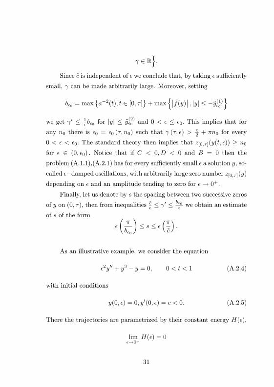
As an illustrative example, we consider the equation

ǫ2y′′ + y3 − y = 0, 0 < t < 1 (A.2.4)

with initial conditions

y(0, ǫ) = 0, y′(0, ǫ) = c < 0. (A.2.5)

There the trajectories are parametrized by their constant energy H(ǫ),

limǫ→0+

H(ǫ) = 0

31

y

w

−√

2√

2y(1)ǫ0

y(2)ǫ0

H = 0

H(ǫ0) > 0

Fig. A.2.1 Phase-plane portrait of the problem (A.2.4)

while conservation of energy requires that 12w

2 + V (y) = H(ǫ) (see

Figure A.2.1 ).

The constant becomes

bǫ0 = max

a−2(t), t ∈ [0, 1]

+ max

∣

∣f(y)∣

∣ , |y| ≤ y(2)ǫ0

= 1 +

√

1 + 2 (ǫ0c)2.

Therefore, γ (1, ǫ0) <3π2 , for instance, when

|c| <√

2π

4and ǫ0 >

[

(π

2

)2

− 2c2]− 1

2

.

On the basis of the considerations above we conclude that for every

n0 ∈ N there is an ǫ0 such that for ǫ ∈ (0, ǫ0) the corresponding solution

has a zero number z[0,1] (y(t, ǫ)) ≥ n0.

References

1. R. Aris: The mathematical theory of diffusion and reaction in permeable

catalysts, Clarendon Press, Oxford, 1975.

32

2. J. A. Boa: A Model Biochemical Reaction, Doctoral Dissertation, Cali-

fornia Institute of Technology, 1974.

3. E. A. Coddington, N. Levinson: Theory of Ordinary Differential Equa-

tions, Krieger Publishing, Malabar, 1984.

4. N. Minorski : Nonlinear Oscillations, Van Nostrand, New Jersey, 1962.

5. D. W. McLaughlin: Path integrals, asymptotics, and singular perturba-

tions, J. Math. Physics 12 (1972), pp. 786–796.

6. D. W. McLaughlin: Complex time, contour independent path integral,

and barrier penetration, J. Math. Physics 12 (1972), pp. 1099–1108.

7. F. C. Moon: Chaotic Vibrations, Wiley, New York, 1987.

8. A. M. Sanches, J. D. Bejarano, D. C. Marzal: Solution of the anhar-

monic quartic potential oscillator problem, J. Sound and Vibration,161(1)

(1993), pp. 19–31.

9. S. Timoshenko, D. H. Young, and W. Weaver, Jr: Vibration Problems in

Engineering, Wiley, New York, 1990.

10. R. Vrábeľ: Singularly pertubed anharmonic quartic potential oscillator

problem, Zeitschrift für angewandte Mathematik und Physik ZAMP. -

ISSN 0044-2275. - Vol. 55 (2004), pp. 720–724.

11. J. Weidmann: Spectral theory of ordinary differential operators, Lecture

Notes in Mathematics 1258, Springer-Verlag, 1987.

33

B SOLUTIONS WITH ARBITRARILY LARGE ZERO

NUMBERS

B.1 Introduction

We consider the second order singularly perturbed differential equa-

tion

ǫ2(

a2(t)y′)′

+ p(t)f(y) = 0, 0 < t < τ, ǫ > 0 (B.1.1)

with initial conditions

y(0, ǫ) = 0, y′(0, ǫ) =c

ǫ, c ∈ R \ 0 (B.1.2)

where

a : [0, τ ] → (0,∞)

is C1 nonincreasing function,

p is C1 decreasing function, p(t) ≥ 0 on [0, τ ],

f is a continuous odd function with exactly three simple zeros

f (−y0) = f(0) = f (y0) = 0, f ′(0) < 0 and limy→∞

f(y)

y<∞.

35

Without loss of generality, we may consider that f is increasing on

(y0,∞) and as a illustrative example, we can take f(y) = y− 2 arctan y

(i.e. (±y0, 0) be the nonhyperbolic equilibria). For hyperbolic theory see

[3] (in this work the author’s consider the FitzHugh-Nagumo equation

with a specific choice of f , f(y) = y(1− y)(y− a), where a > 0 is a real

parameter), [2], for example.

For the singular problem, that is, when ǫ→ 0+, the considerations

as below may be relevant to the study of equilibrium solutions of the

scalar parabolic reaction-diffusion equation with decreasing diffusion.

Also, we remark that for p ≥ 0 the corresponding equation is not dis-

sipative. Moreover, this class of equations has special significance in

connection with applications involving nonlinear vibrations and chaos

(e.g. references [4], [5], [7]).

The problems of this form have been previously considered by

Rocha [6] and Angenent et al. [1]. In [6], p(t) ≡ −1. However, the situ-

ation is more complicated when p(t) ≥ 0 from the existence of the zeros

of solutions point of view. It follows from the fact that the linearized

version of (B.1.1) do not admit an oscillatory solution for p(t) ≥ 0,

unlike the case p(t) < 0.

The goal of this chapter is to prove the existence of decreasing

sequence ǫn∞n=n0, ǫn → 0+ such that the corresponding solutions of

(B.1.1),(B.1.2) have n zeros on (0, τ) for every n ≥ n0, n ∈ N and

y (τ, ǫn) = 0.

Nomenclature

f(y) = f(y)yfor y 6= 0 and f(0) = f ′(0);

36

V (y) =y∫

0

f(u)du;

z[0,τ ](y) denotes the zero number of the nontrivial solution y of

(B.1.1) on (0, τ);

−Ys,ǫ, Ys,ǫ (−Ys,ǫ < Ys,ǫ) denote the real roots of equation

p(s)V (y) = H(s, y(s, ǫ), w(s, ǫ), ǫ) − r(s, ǫ)

for s ∈ [0, τ ] (for definition of H and r see below);

−Y0, 0, Y0 (−Y0 < 0 < Y0) denote the real roots of equation V (y) =

0;

dI(y) denotes spacing between two successive zero numbers of y

on the interval I.

The rest of this chapter is organized as follows. In Section B.2 is ex-

plained technique necessary for the understanding of the chapter and in

Section B.3 is formulated the theorem which is the main result.

B.2 Preliminaries

In order to apply the standard approach for the study of the so-

lutions of (B.1.1) we introduce the variable w = ǫay′ and write this

equation in the system form

y′ =1

ǫaw (B.2.1)

w′ =− 1

ǫap(t)f(y) − a′

aw. (B.2.2)

If we consider the function

H(t, y, w, ǫ) = H(t, y, w) + r(t, ǫ)

37

where

H(t, y, w) =1

2w2 + p(t)V (y),

r(t, ǫ) = −t∫

0

p′ (s)

y(s,ǫ)∫

0

f (u)du

ds

and compute its derivative along the solutions of (B.2.1), (B.2.2), we

have

˙H(t, y, w, ǫ) = ww′ + p(t)f(y)y′ + p′(t)

y∫

0

f(u)du+ r′(t, ǫ)

= w

[

− 1

ǫap(t)f(y) − a′

aw

]

+ p(t)f(y)y′ + p′(t)

y∫

0

f(u)du+ r′(t, ǫ)

= −a′

aw2.

Hence, we conclude that H is monotone, nondecreasing function and

H

t=0= 1

2 (a(0)c)2> 0 implies that H > 0 on [0, τ ] for every ǫ. We use

the level curves of H to characterize the trajectories of (B.2.1), (B.2.2).

One first draws the (t, y)− p(t)V (y) profile and then graphically draws

the trajectory (y, w) with

w = ±(

2(

H − r(t, ǫ) − p(t)V (y)))

12

extending it as long as w remains real (i.e., until p(t)V (y) exceeds H−r).It is instructive for the future to keep in the mind the phase-portraits

of the system (B.2.1), (B.2.2) with H − r ≥ 0 (see Figure B.2.1 ).

Let us introduce the new variable v = ǫa2y′ and write (B.1.1) in

the system form

y′ =1

ǫa2v (B.2.3)

v′ =−1

ǫp(t)f(y). (B.2.4)

38

y

w

−Y0 Y0−Ys,ǫ∗ Ys,ǫ∗

Fig. B.2.1 Intersection a 3-dimensional manifold12w

2 + p(s)V (y) = H − r with the subspace (t, y) = (s, ǫ∗) of

(t, y, w, ǫ)-space for H − r > 0

Then, expressing (y, v) in polar coordinates, y = r cos γ, v = −r sin γ

(obviously, y2+v2 > 0 for every nontrivial solution of (B.1.1)) we obtain

the following differential equation for γ

γ′ =1

ǫ

[

1

a2(t)sin2 γ + p(t)f(y(t, ǫ)) cos2 γ

]

, (B.2.5)

γ(0) = π2 (for c < 0) or γ(0) = 3π

2 (for c > 0). It is clear, that γ(1, ǫ) >

(2k + 1)π2 , k ∈ N implies that z[0,τ ](y(t, ǫ) > k (for c < 0).

B.3 Main result

We precede the main result of this chapter by important Lemma.

Lemma 1. H − r ≥ 0 on [0, τ ], H − r > 0 for y ∈ (−Y0, Y0).

39

Proof. The statement follows immediately from the inequalities(

H − r)′

= p′V − a′

aw2 ≥ p′V > 0

for y ∈ (−Y0, Y0) and

H − r > 0

for y ∈ [−Yt,ǫ, Yt,ǫ] \ [−Y0, Y0] .

Now we formulate the main result of this chapter.

Theorem 1. (see, e.g., [8]) Consider the problem (B.1.1),

(B.1.2). Assume that

f(y)

y>

2V (y)

y2for every y ∈ [−y0, y0] \ 0. (B.3.1)

Then there is a decreasing sequence ǫn∞n=n0, lim

n→∞ǫn = 0 such that

(i) The corresponding solution of (B.1.1), (B.1.2) has

z[0,τ ] (y (t, ǫn)) = n

.

(ii) h1 (t, ǫn) ≤ dI (y (t, ǫn)) ≤ h2 (t, ǫn) ,

where h1 (t, ǫn) = O (ǫn), h2 (t, ǫn) = O (ǫn) and I ⊂ [0, τ ] is connected

and closed.

Proof. Using the identity cos2 γ + sin2 γ = 1, from (B.2.5) we obtain

γ′ =1

ǫ

[

1

a2+ cos2 γ

(

p(t)f(y) − 1

a2

)]

.

Let ξ ∈ [0, τ ]. The definition of polar coordinates implies that cos2 γ =y2

y2+v2 = y2

y2+a2w2 . Thus,

∣

∣

∣

∣

cos2 γ

(

pf − 1

a2

)∣

∣

∣

∣

=

∣

∣

∣

∣

∣

y2(

pf − 1a2

)

y2 + v2

∣

∣

∣

∣

∣

=

∣

∣

∣

∣

∣

y2(

pf − 1a2

)

y2 + 2a2(H − r − pV )

∣

∣

∣

∣

∣

40

for y ∈ [−Yξ,ǫ, Yξ,ǫ].

Because H − r > 0, there is a positive constant κ1 independent of ǫ,

κ1 < y0 such that∣

∣

∣

∣

cos2 γ

(

p(ξ)f − 1

a2(ξ)

)∣

∣

∣

∣

<1

2a2(ξ)

for |y| < κ1. Further for |y| ≥ κ1, taking into consideration the conclu-

sions of Lemma, we obtain

∣

∣

∣

∣

cos2 γ

(

p(ξ)f − 1

a2(ξ)

)∣

∣

∣

∣

≤∣

∣

∣

∣

∣

y2(

a−2(ξ) − p(ξ)f(y))

y2 − 2a2(ξ)p(ξ)V (y)

∣

∣

∣

∣

∣

.

From the condition (B.3.1) we conclude that

0 <a−2(ξ) − p(ξ)f(y)

a−2(ξ) − 2p(ξ)V (y)y2

< 1

and after little arrangement we get

0 <y2(

a−2(ξ) − p(ξ)f(y))

y2 − 2a2(ξ)p(ξ)V (y)<

1

a2(ξ)

for κ1 ≤ |y| ≤ y0 + κ2 < Y0, where κ2 is a sufficiently small positive

constant.

Let c(ξ) = min c1(ξ), c2(ξ) , where

c1(ξ) = min

1

a2(ξ)− y2

(

a−2(ξ) − p(ξ)f(y))

y2 − 2a2(ξ)p(ξ)V (y), |y| ≤ y0 + κ2

,

c2(ξ) = min

1

a2(ξ)sin2 γ + p(ξ)f(y) cos2 γ,

y0 + κ2 ≤ |y| ≤ Yξ,ǫ, γ ∈ R

and we define for t ∈ [0, τ0) the function

c(t) = min c(ξ); ξ ∈ [0, t] .

41

Clearly, c(t) is a positive nonincreasing function on [0, τ ] except that

c(τ) = 0 if p(τ) = 0. Hence, γ′ ≥ c(t)ǫfor t ∈ [0, τ ]. Since c(t) is

independent of ǫ we conclude that, by taking ǫ sufficiently small, γ can

be made arbitrarily large, γ(τ, ǫ) ≥ π2 + 1

ǫ

∫ τ

0c(u)du for c < 0.

Moreover, setting

c∗(t) = a−2(t) + sup

p(t)f(y); t ∈ [0, τ ], y ∈ R

on [0, τ ] , we get γ′ ≤ c∗(t)ǫfor t ∈ [0, τ ]. The continuity of γ with

respect to a parameter ǫ, ǫ 6= 0 we obtain such values ǫ that γ (τ, ǫn) =π2 +πn. for every n ≥ n0. The corresponding solution of (B.1.1), (B.1.2)

has a zero number z[0,τ ] (y (t, ǫn)) = n − 1. This completes the proof

of statement (i). Integrating between two successive zero numbers of

solution y(t, ǫ) on an interval I ⊂ [0, τ ] (if p(τ) = 0 then I ⊂ [0, τ)), we

obtain an estimate of dI (y(t, ǫn)) of the form

ǫn

(

π

c∗I

)

≤ dI (y(t, ǫn)) ≤ ǫn

(

π

cI

)

,

where c∗I = supt∈I

c∗(t) and cI = inft∈I

c(t). Theorem is proven.

Remark 1. Oddness of f is considered in order to avoid technicalities,

and is not essential. Ones modify the theorem for a general function f

with three undegenerate zeros and satisfying 0 ≤ lim supy→∞

f(y)y

<∞.

References

1. S. Angenent, J. Mallet-Paret and L. Peletier: Stable transitions layers

in a semilinear boundary value problem, J. Differential Equations Vol. 67

(1989), pp. 212–242.

2. Ch. K.R.T. Jones: Geometric Singular Perturbation Theory, C.I.M.E

Lectures, Session on Dynamical Systems, 1994.

42

3. C. Krupa, B. Sandstede and P. Szmolyan: Fast and Slow Waves in the

FitzHugh-Nagumo Equation, J. Math. Anal. Appl., Vol. 133 (1997), pp.

49–97.

4. N. Minorski : Nonlinear Oscillations, Van Nostrand, New Jersey, 1962.

5. F. C. Moon: Chaotic Vibrations, Wiley, New York, 1987.

6. C. Rocha: On the Singular problem for the Scalar Parabolic Equation with

Variable Diffusion, J. Math. Anal. Appl., Vol. 183 (1994), pp. 413–428.

7. S. Timoshenko, D. H. Young and W. Weaver, Jr.: Vibration Problems in

Engineering, Wiley, New York, 1990.

8. R. Vrabel: On the solutions of differential equation

ǫ2

`

a2(t)y′

´′

+ p(t)f(y) = 0

with arbitrarily large zero number, Journal of Computational Analysis

and Applications. - ISSN 1521-1398. - Vol. 6, No. 2 (2004), pp. 139–146.

43

C THREE-POINT BOUNDARY VALUE PROBLEM

C.1 Introduction

We will consider the three point problem

ǫy′′ + ky = f(t, y), t ∈ 〈a, b〉, k < 0, 0 < ǫ << 1 (C.1.1)

y′(a) = 0, y(b) − y(c) = 0, a < c < b (C.1.2)

This is singular perturbation problem because the order of differ-

ential equation drops when ǫ becomes zero. The situation in the present

case is complicated by the fact that there are the inner points in the

boundary conditions, on the difference with the”standard“ boundary

conditions as Dirichlet problem, Neumann problem, Robin problem, pe-

riodic boundary value problem ([2], [3]), for example.

We apply the method of upper and lower solutions and the delicate es-

timates to prove the existence of a solution for problem (C.1.1), (C.1.2)

which converges uniformly to the solution of reduced problem (i.e. if

we let ǫ → 0+ in (C.1.1)) on every compact subset of interval 〈a, b) forǫ→ 0+.

As usual, we say that αǫ ∈ C2(〈a, b〉) is a lower solution for prob-lem (C.1.1), (C.1.2) if ǫα′′

ǫ (t) + kαǫ(t) ≥ f(t, αǫ(t)) and α′ǫ(0) = 0,

45

αǫ(b) − αǫ(c) ≤ 0 for every t ∈ 〈a, b〉. An upper solution βǫ ∈ C2(〈a, b〉)satisfies ǫβ′′

ǫ (t) + kβǫ(t) ≤ f(t, βǫ(t)) and β′ǫ(0) = 0, βǫ(b) − βǫ(c) ≥ 0

for every t ∈ 〈a, b〉.

Lemma 1 (cf. [1]). If αǫ, βǫ are lower and upper solutions for (C.1.1),

(C.1.2) such that αǫ ≤ βǫ, then there exists solution yǫ of (C.1.1),

(C.1.2) with αǫ ≤ yǫ ≤ βǫ.

Denote D(u) = (t, y)| a ≤ t ≤ b, |y − u(t)| < d(t) , where d(t) isthe positive continuous function on 〈a, b〉 such that

d(t) =

δ for a ≤ t ≤ b− δ

|u(b) − u(c)| + δ for b− δ2 ≤ t ≤ b

δ is a small positive constant and u ∈ C2 is a solution of reduced problem

ku = f(t, u).

C.2 Existence and asymptotic behavior of solutions

Theorem 1. (see, [4]) Let f ∈ C1(D(u)) satisfies the condition

∣

∣

∣

∣

∂f(t, y)

∂y

∣

∣

∣

∣

≤ w < −k for every (t, y) ∈ D(u). (hyperbolicity)

Then there exists ǫ0 such that for every ǫ ∈ (0, ǫ0〉 the problem(C.1.1), (C.1.2) has a unique solution satisfying the inequality

vǫ(t) − Cǫ ≤ yǫ(t) − (u(t) + vǫ(t)) ≤ −vǫ(t) + C√ǫ (C.2.1)

for u′(a) ≤ 0 and

vǫ(t) − C√ǫ ≤ yǫ(t) − (u(t) + vǫ(t)) ≤ −vǫ(t) + Cǫ (C.2.2)

46

for u′(a) ≥ 0 on 〈a, b〉 where

vǫ(t) = u′(a)

· e√

mǫ

(t−b) − e√

mǫ

(b−t) + e√

mǫ

(c−t) − e√

mǫ

(t−c)

√

mǫ

(

e√

mǫ

(a−c) − e√

mǫ

(a−b) + e√

mǫ

(c−a) − e√

mǫ

(b−a))

vǫ(t) = |u(b) − u(c)|

· e√

mǫ

(t−a) + e√

mǫ

(a−t)

(

e√

mǫ

(a−c) − e√

mǫ

(a−b) + e√

mǫ

(c−a) − e√

mǫ

(b−a)) ,

m = −k − w and C, C are the positive constants.

Proof. The functions vǫ(t) and vǫ(t) on 〈a, b〉 satisfy:

1. ǫv′′ǫ − mvǫ = 0, v′ǫ(a) = −u′(a), vǫ(b) − vǫ(c) = 0, vǫ ≤ 0 for

u′(a) ≤ 0 and vǫ ≥ 0 for u′(a) ≥ 0

2. ǫv′′ǫ −mvǫ = 0, v′ǫ(a) = 0, vǫ(b) − vǫ(c) = −|u(b) − u(c)|, vǫ ≤ 0.

For u′(a) ≤ 0 we define the lower solutions by

αǫ(t) = u(t) + vǫ(t) + vǫ(t) − Γǫ

and the upper solutions by

βǫ(t) = u(t) + vǫ(t) − vǫ(t) + Γǫ

( for u′(a) ≥ 0 we proceed analogously.)

Here Γǫ = ǫ∆mand Γǫ =

√ǫ∆mwhere ∆, ∆ are the constants which

shall be defined below. α ≤ β on 〈a, b〉 and satisfy the boundary condi-tions prescribed for the lower and upper solutions of (C.1.1), (C.1.2).

Now we show that ǫα′′ǫ (t) + kαǫ(t) ≥ f(t, αǫ(t)) and ǫβ′′

ǫ (t) +

kβǫ(t) ≤ f(t, βǫ(t)). Denote h(t, y) = f(t, y)−ky. By the Taylor theorem

47

we obtain

h(t, αǫ(t)) = h(t, αǫ(t)) − h(t, u(t))

=∂h(t, θǫ(t))

∂y(vǫ(t) + vǫ(t) − Γǫ)

where (t, θǫ(t)) is a point between (t, αǫ(t)) and (t, u(t)), and (t, θǫ(t)) ∈D(u) for sufficiently small ǫ. Hence

ǫα′′ǫ (t) − h(t, αǫ(t)) ≥ ǫu′′ + ǫv′′ǫ (t) + ǫv′′ǫ (t) −m(vǫ(t) + vǫ(t) − Γǫ)

≥ −ǫ|u′′| + ǫ∆.

If we choose a constant ∆ such that ∆ ≥ |u′′(t)|, t ∈ 〈a, b〉 then ǫα′′ǫ (t) ≥

h(t, αǫ(t)) in 〈a, b〉.Inequality for βǫ(t)) :

h(t, βǫ(t)) − ǫβ′′ǫ (t) =

∂h(t, θǫ(t))

∂y(vǫ(t) − vǫ(t) + Γǫ) − ǫβ′′

ǫ (t)

=∂h(t, θǫ(t))

∂y(vǫ(t) − vǫ(t) + Γǫ) − ǫ(u′′ + v′′ǫ (t) − v′′ǫ (t))

≥ ∂h(t, θǫ(t))

∂yvǫ(t) +mΓǫ − ǫu′′ − ǫv′′ǫ (t)

=

(

∂h(t, θǫ(t))

∂y−m

)

vǫ(t) +mΓǫ − ǫu′′.

Let L = max|u′′(t)| |t ∈ 〈a, b〉 and denote vǫ = vǫ√ǫ. Then ǫβ′′

ǫ (t) ≤h(t, βǫ(t)) if

mΓǫ − ǫL ≥(

∂h(t, θǫ(t))

∂y−m

)

|vǫ(t)|

i.e.√ǫ(

∆ −√ǫL)

≥(

∂h(t, θǫ(t))

∂y−m

)

√ǫ|vǫ(t)|

48

∆ ≥√ǫL+

(

∂h(t, θǫ(t))

∂y−m

)

|vǫ(t)|

Thus, from the inequalities m ≤ ∂h(t,θǫ(t))∂y

≤ m+ 2w in D(u) and

vǫ(t) ≤ 0 follows that it is sufficient to choose a constant ∆ such that

∆ ≥√ǫL+ 2w

|u′(a)|√m

.

The existence of a solution for (C.1.1), (C.1.2) satisfying the above

inequality follows from Lemma 1.

Remark 2. Theorem 1 implies that yǫ(t) = u(t) + O(√ǫ) on every

compact subset of 〈a, b) and limǫ→0+

yǫ(b) = u(c). Boundary layer effect

occurs at the point b in the case, when u(c) 6= u(b).

References

1. J. Mawhin: Points fixes, points critiques et problemes aux limites, Semin.

Math. Sup. no. 92, Presses Univ. Montreal, 1985.

2. R. Vrábeľ: Asymptotic behavior of T-periodic solutions of singularly

perturbed second-order differential equation, Mathematica Bohemica 121

(1996), pp. 73—76.

3. R. Vrábeľ: Semilinear singular perturbation, Nonlinear analysis, TMA. -

ISSN 0362-546X. - Vol. 25, No. 1 (1995), pp. 17–26.

4. R. Vrábeľ: Three point boundary value problem for singularly perturbed

semilinear differential equations, E. J. Qualitative Theory of Diff. Equ. -

ISSN: 1417–3875. - No. 70 (2009), pp. 1–4.

49

D FOUR-POINT BOUNDARY VALUE PROBLEM

D.1 Preliminaries

We will consider the four (or three) point boundary value problem

ǫy′′ + ky = f(t, y), t ∈ 〈a, b〉, k < 0, 0 < ǫ << 1 (D.1.1)

y(c) − y(a) = 0, y(b) − y(d) = 0, a < c ≤ d < b. (D.1.2)

We can view this equation as the mathematical model of the nonlin-

ear dynamical system with a high-speed feedback. Moreover, this class

of equations has special significance in connection with applications in-

volving nonlinear vibrations. We focus on the existence and asymptotic

behavior of a solutions yǫ(t) for ǫ belonging to a non-resonant set and

on an estimate of the difference between the solution yǫ(t) of (D.1.1),

(D.1.2) and a singular solution u(t) of the equation ku = f(t, u).

The situation in the present case is complicated by the fact that

there are the inner points in the boundary conditions, in contrast to

the boundary conditions as the Dirichlet problem, Neumann problem,

Robin problem, periodic boundary value problem ([1, 2, 5, 6, 9]), for

example. In the problem considered there does not exist a positive

51

solution vǫ of Diff. Eq. ǫy′′ −my = 0, m > 0, 0 < ǫ (i.e. vǫ is convex)

such that vǫ(c) − vǫ(a) = u(c) − u(a) > 0 and vǫ(t) → 0+ for t ∈ (a, b〉and ǫ → 0+, which could be used to solve this problem by the method

of upper and lower solutions. We will define the correction function

v(corr)ǫ (t) which will allow us to apply the method.

As was said before, we apply the method of upper and lower so-

lutions and some delicate estimates to prove the existence of a solution

for problem (D.1.1), (D.1.2) which converges uniformly to the solution

u of the reduced problem (i.e. if we let ǫ → 0+ in (D.1.1)) on every

compact subset of interval (a, b) for ǫ → 0+. Moreover, we give the

accurate numerical approximation of solutions up to order O(ǫ). The

regular case, when ǫ = 1, for the difference equations with three-point

time scale boundary value conditions was studied in [3].

As usual, we say that αǫ ∈ C2(〈a, b〉) is a lower solution for problem(D.1.1), (D.1.2) if ǫα′′

ǫ (t) + kαǫ(t) ≥ f(t, αǫ(t)) and αǫ(c) − αǫ(a) = 0,

αǫ(b)− αǫ(d) ≤ 0 for every t ∈ 〈a, b〉. An upper solution βǫ ∈ C2(〈a, b〉)satisfies ǫβ′′

ǫ (t) + kβǫ(t) ≤ f(t, βǫ(t)) and βǫ(c) − βǫ(a) = 0, βǫ(b) −βǫ(d) ≥ 0 for every t ∈ 〈a, b〉.

Lemma 1 ([4]). If αǫ, βǫ are respectively lower and upper solutions

for (D.1.1), (D.1.2) such that αǫ ≤ βǫ, then there exists solution yǫ of

(D.1.1), (D.1.2) with αǫ ≤ yǫ ≤ βǫ.

Denote H(u) = (t, y)| a ≤ t ≤ b, |y − u(t)| < d(t) , where d(t) isthe positive continuous function on 〈a, b〉 such that

d(t) =

|u(c) − u(a)| + δ for a ≤ t ≤ a+ δ2

δ for a+ δ ≤ t ≤ b− δ

|u(b) − u(d)| + δ for b− δ2 ≤ t ≤ b

52

δ is a small positive constant and u ∈ C2 is a solution of the re-

duced problem ku = f(t, u). We will write s(ǫ) = O(r(ǫ)) when 0 <

limǫ→0+

∣

∣

∣

s(ǫ)r(ǫ)

∣

∣

∣ <∞.

D.2 Main result

Theorem 1. (see, e.g., [7, 8]) Let f ∈ C1(H(u)) satisfies the condi-

tion∣

∣

∣

∣

∂f(t, y)

∂y

∣

∣

∣

∣

≤ w < −k for every (t, y) ∈ H(u) (hyperbolicity).

Then there exists ǫ0 such that for every ǫ ∈ (0, ǫ0〉 the problem(D.1.1), (D.1.2) has a unique solution satisfying the inequality

−v(corr)ǫ (t) − vǫ(t) − Cǫ ≤ yǫ(t) − (u(t) + vǫ(t)) ≤ vǫ(t) + Cǫ

for u(c) − u(a) ≥ 0 and

−vǫ(t) − Cǫ ≤ yǫ(t) − (u(t) + vǫ(t)) ≤ v(corr)ǫ (t) + vǫ(t) + Cǫ

for u(c) − u(a) ≤ 0 on 〈a, b〉 where

vǫ(t) =u(c) − u(a)

D

·(

e√

mǫ

(b−t) − e√

mǫ

(t−b) + e√

mǫ

(t−d) − e√

mǫ

(d−t))

,

vǫ(t) =|u(b) − u(d)|

D

·(

e√

mǫ

(t−a) − e√

mǫ

(a−t) + e√

mǫ

(c−t) − e√

mǫ

(t−c))

,

D =(

e√

mǫ

(b−a) + e√

mǫ

(d−c) + e√

mǫ

(c−b) + e√

mǫ

(a−d))

−(

e√

mǫ

(a−b) + e√

mǫ

(c−d) + e√

mǫ

(b−c) + e√

mǫ

(d−a))

,

53

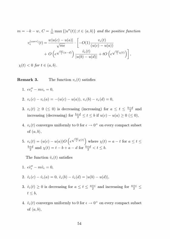
m = −k−w, C = 1m

max |u′′(t)| ; t ∈ 〈a, b〉 and the positive function

v(corr)ǫ (t) =

w|u(c) − u(a)|√mǫ

·[

−O(1)vǫ(t)

(u(c) − u(a))

+ O(

e√

mǫ

(a−d)) vǫ(t)

|u(b) − u(d)| + tO(

e√

mǫ

χ(t))

]

,

χ(t) < 0 for t ∈ (a, b〉.

Remark 3. The function vǫ(t) satisfies

1. ǫv′′ǫ −mvǫ = 0,

2. vǫ(c) − vǫ(a) = −(u(c) − u(a)), vǫ(b) − vǫ(d) = 0,

3. vǫ(t) ≥ 0 (≤ 0) is decreasing (increasing) for a ≤ t ≤ b+d2 and

increasing (decreasing) for b+d2 ≤ t ≤ b if u(c) − u(a) ≥ 0 (≤ 0),

4. vǫ(t) converges uniformly to 0 for ǫ→ 0+ on every compact subset

of (a, b〉,

5. vǫ(t) = (u(c) − u(a))O(

e√

mǫ

χ(t))

where χ(t) = a− t for a ≤ t ≤b+d2 and χ(t) = t− b+ a− d for b+d

2 < t ≤ b.

The function vǫ(t) satisfies

1. ǫv′′ǫ −mvǫ = 0,

2. vǫ(c) − vǫ(a) = 0, vǫ(b) − vǫ(d) = |u(b) − u(d)|,

3. vǫ(t) ≥ 0 is decreasing for a ≤ t ≤ a+c2 and increasing for a+c

2 ≤t ≤ b,

4. vǫ(t) converges uniformly to 0 for ǫ→ 0+ on every compact subset

of 〈a, b),

54

5. vǫ(t) = |u(b) − u(d)|O(

e√

mǫ

χ(t))

where χ(t) = c − b + a − t for

a ≤ t < a+c2 and χ(t) = t− b for a+c

2 ≤ t ≤ b.

The correction function v(corr)ǫ (t) will be determined precisely in the

next section.

D.3 The correction function v(corr)ǫ (t)

Consider the linear problem

ǫy′′ −my = −2w |vǫ(t)| , t ∈ 〈a, b〉, ǫ > 0 (D.3.1)

with the boundary condition (D.1.2).

We apply the method of upper and lower solutions. We define

αǫ(t) = 0

and

βǫ(t) =2w

mmax |vǫ(t)| , t ∈ 〈a, b〉 =

2w

m|vǫ(a)| .

Obviously, |vǫ(a)| = 2wm|u(c) − u(a)|

(

1 + O(

e√

mǫ

(a−c)))

and the con-

stant functions α, β satisfy the differential inequalities required on the

upper and lower solutions for (D.3.1) and the boundary conditions for

(D.1.2). Thus on the basis of Lemma 1 there exists unique solution yLinǫ

of linear problem with (D.1.2) for every ǫ such that

0 ≤ yLinǫ (t) ≤ 2w

m|u(c) − u(a)|

(

1 + O(

e√

mǫ

(a−c)))

on 〈a, b〉. The solution we denote by v(corr)ǫ (t), i.e. the function

v(corr)ǫ (t)

def= yLin

ǫ (t)

55

and we compute v(corr)ǫ (t) exactly:

v(corr)ǫ (t) = − (ψǫ(a) − ψǫ(c))

(u(c) − u(a))vǫ(t) +

(ψǫ(d) − ψǫ(b))

|u(b) − u(d)| vǫ(t) + ψǫ(t)

where

ψǫ(t) =w|u(c) − u(a)|

D√mǫ

t

·(

e√

mǫ

(b−t) + e√

mǫ

(t−b) − e√

mǫ

(d−t) − e√

mǫ

(t−d))

.

Hence

ψǫ(a)− ψǫ(c) =w|u(c) − u(a)|

D√mǫ

a

·(

e√

mǫ

(b−a) + e√

mǫ

(a−b) − e√

mǫ

(d−a) − e√

mǫ

(a−d))

− w|u(c) − u(a)|D√mǫ

c

·(

e√

mǫ

(b−c) + e√

mǫ

(c−b) − e√

mǫ

(d−c) − e√

mǫ

(c−d))

=w|u(c) − u(a)|√

mǫO(1),

ψǫ(d)− ψǫ(b) =w|u(c) − u(a)|

D√mǫ

d(

e√

mǫ

(b−d) + e√

mǫ

(d−b) − 2)

− w|u(c) − u(a)|D√mǫ

b(

2 − e√

mǫ

(d−b) − e√

mǫ

(b−d))

=w|u(c) − u(a)|√

mǫO(

e√

mǫ

(a−d))

,

ψǫ(t) =w|u(c) − u(a)|√

mǫO(

e√

mǫ

χ(t))

.

Thus, we obtain

v(corr)ǫ (t) =

w|u(c) − u(a)|√mǫ

·[

−O(1)vǫ(t)

(u(c) − u(a))

+ O(

e√

mǫ

(a−d)) vǫ(t)

|u(b) − u(d)| + tO(

e√

mǫ

χ(t))

]

.

56

D.4 Proof of Theorem

First we will consider the case u(c) − u(a) ≥ 0. We define the

lower solutions by

αǫ(t) = u(t) + vǫ(t) − v(corr)ǫ (t) − vǫ(t) − Γǫ

and the upper solutions by

βǫ(t) = u(t) + vǫ(t) + vǫ(t) + Γǫ.

Here Γǫ = ǫ∆mwhere ∆ is the constant which shall be defined below,

α ≤ β on 〈a, b〉 and satisfy the boundary conditions prescribed for thelower and upper solutions of (D.1.1), (D.1.2).

Now we show that ǫα′′ǫ (t) + kαǫ(t) ≥ f(t, αǫ(t)) and ǫβ′′

ǫ (t) +

kβǫ(t) ≤ f(t, βǫ(t)). Denote h(t, y) = f(t, y)−ky. By the Taylor theoremwe obtain

h(t, αǫ(t)) = h(t, αǫ(t)) − h(t, u(t))

=∂h(t, θǫ(t))

∂y(vǫ(t) − v(corr)

ǫ (t) − vǫ(t) − Γǫ),

where (t, θǫ(t)) is a point between (t, αǫ(t)) and (t, u(t)), and (t, θǫ(t)) ∈H(u) for sufficiently small ǫ.Hence, from the inequalitiesm ≤ ∂h(t,θǫ(t))

∂y≤

m+ 2w in H(u) we have

ǫα′′ǫ (t) − h(t, αǫ(t)) ≥

ǫu′′(t) + ǫv′′ǫ (t) − ǫv(corr)′′

ǫ (t) − ǫv′′ǫ (t) − (m+ 2w)vǫ(t)

+mv(corr)ǫ (t) +mvǫ(t) +mΓǫ.

Because vǫ(t) = |vǫ(t)| we have

−ǫv(corr)′′

ǫ (t) − 2wvǫ(t) +mv(corr)ǫ (t) = 0,

57

as follows from Diff. Eq. (D.3.1), we get

ǫα′′ǫ (t) − h(t, αǫ(t)) ≥ ǫu′′(t) +mΓǫ ≥ −ǫ|u′′(t)| + ǫ∆.

For βǫ(t)) we have the inequality

h(t, βǫ(t)) − ǫβ′′ǫ (t) =

∂h(t, θǫ(t))

∂y(vǫ(t) + vǫ(t) + Γǫ) − ǫβ′′

ǫ (t)

= m(vǫ(t) + vǫ(t) + Γǫ) − ǫ(u′′(t) + v′′ǫ (t) + v′′ǫ (t)) ≥ ǫ∆ − ǫ|u′′(t)|

where (t, θǫ(t)) is a point between (t, u(t)) and (t, βǫ(t)) and (t, θǫ(t)) ∈H(u) for sufficiently small ǫ.

The case u(c) − u(a) ≤ 0:

The lower solutions

αǫ(t) = u(t) + vǫ(t) − vǫ(t) − Γǫ

and the upper solutions

βǫ(t) = u(t) + vǫ(t) + v(corr)ǫ (t) + vǫ(t) + Γǫ

satisfy

ǫα′′ǫ − h(t, αǫ)

= ǫu′′ + ǫv′′ǫ − ǫv′′ǫ − ∂h

∂y(vǫ − vǫ − Γǫ)

= ǫu′′ + ǫv′′ǫ − ǫv′′ǫ +∂h

∂y(−vǫ + vǫ + Γǫ)

≥ ǫu′′ + ǫv′′ǫ − ǫv′′ǫ +m(−vǫ + vǫ + Γǫ) = ǫu′′ + ǫ∆

≥ ǫ∆ − ǫ|u′′|

h(t, βǫ) − ǫβ′′ǫ

58

=∂h

∂y

(

vǫ + v(corr)ǫ + vǫ + Γǫ

)

− ǫu′′ − ǫv′′ǫ − ǫv(corr)′′

ǫ − ǫv′′ǫ

≥ (m+ 2w)vǫ +m(

v(corr)ǫ + vǫ + Γǫ

)

− ǫu′′ − ǫv′′ǫ − ǫv(corr)′′

ǫ − ǫv′′ǫ

= −2w |vǫ| +mv(corr)ǫ − ǫv(corr)′′

ǫ + ǫ∆ − ǫu′′ = ǫ∆ − ǫu′′

≥ ǫ∆ − ǫ|u′′|.

Now, if we choose a constant ∆ such that ∆ ≥ |u′′(t)|, t ∈ 〈a, b〉then ǫα′′

ǫ (t) ≥ h(t, αǫ(t)) and ǫβ′′ǫ (t) ≤ h(t, βǫ(t)) in 〈a, b〉.

The existence of a solution for (D.1.1), (D.1.2) satisfying the above

inequality follows from Lemma 1. The uniqueness of solutions follows

from the fact that the function h(t, y) is increasing in the variable y in

H(u) (Peano’s phenomenon).

Remark 4. Theorem 1 implies that yǫ(t) = u(t) + O(ǫ) on every

compact subset of (a, b) and limǫ→0+

yǫ(a) = u(c), limǫ→0+

yǫ(b) = u(d). The

boundary layer effect occurs at the point a or/and b in the case when

u(a) 6= u(c) or/and u(b) 6= u(d).

D.5 Approximation of the solutions

In this section the case u(c) − u(a) ≥ 0 will be considered only.

For u(c)−u(a) ≤ 0 we proceed analogously. We define the approximate

solution yǫ(t) of (D.1.1), (D.1.2) by

yǫ(t) =1

2(αǫ(t) + βǫ(t)) = u(t) + vǫ(t) −

v(corr)ǫ (t)

2.

Taking into consideration the conclusions of Theorem 1, in both

cases we obtain the following estimate for the solution yǫ of problem

(D.1.1), (D.1.2)

59

|yǫ(t) − yǫ(t)| ≤ vǫ(t) +v(corr)ǫ (t)

2+

ǫ

mmax |u′′(t)| , t ∈ 〈a, b〉 .

References

1. K. W. Chang and F. A. Howes: Nonlinear Singular perturbation phenom-

ena: Theory and Applications, Springer-Verlag, New York, 1984.

2. C. De Coster and P. Habets: Two-Point Boundary Value Problems:

Lower and Upper Solutions, Volume 205 (Mathematics in Science and

Engineering), Elsevier Science; 1 edition, 2006.

3. R. A. Khan, J. Nieto and V. Otero-Espinar: Existence and approximation

of solution of three-point boundary value problems on time scales, Journal

of Difference Equations and Applications, Volume 14 (2008), Number 7,

pp. 723–736(14).

4. J. Mawhin: Points fixes, points critiques et problemes aux limites, Semin.

Math. Sup. no. 92, Presses Univ. Montreal, 1985.

5. R. Vrábeľ: Asymptotic behavior of T-periodic solutions of singularly

perturbed second-order differential equation, Mathematica Bohemica 121

(1996), pp. 73-–76.

6. R. Vrábeľ: Semilinear singular perturbation, Nonlinear Analysis, TMA. -

ISSN 0362-546X. - Vol. 25 (1995), No. 1, pp. 17–26.

7. R. Vrábeľ: Nonlocal Four-Point Boundary Value Problem for the Singu-

larly Perturbed Semilinear Differential Equations, Boundary value prob-

lems. - ISSN 1687-2762. - Article ID 570493 (2011), 70493–70493.

8. R. Vrábeľ: A priori estimates for the solutions of a four point boundary

value problem for the singularly perturbed semilinear differential equa-

tions, Electron. J. Diff. Equ. - ISSN 1072-6691. - Vol. 2011 (2011), No.

21, pp. 1–7.

60

9. B. Q. Yan, D. O’Regan and R. P. Agarwal: Positive Solutions to Singular

Boundary Value Problems with Sign Changing Nonlinearities on the Half-

Line via Upper and Lower Solutions, Acta Mathematica Sinica, English

Series, Vol. 23 (2007), No. 8, pp. 1447-–1456.

61

E BOUNDARY LAYER PHENOMENON

E.1 Introduction

In various fields of science and engineering, systems with two-time-

scale dynamics are often investigated. In state space, such systems are

commonly modeled using the mathematical framework of singular per-

turbations, with a small parameter, say ǫ, determining the degree of

separation between the ”slow” and ”fast” channels of the system. Sin-

gularly perturbed systems (SPSs) may occur also due to the presence of

small ”parasitic” parameters, armature inductance in a common model

for most DC motors, small time constants, etc.

The literature on control of nonlinear SPSs is extensive, at least

starting with the pioneering work [3] of P. Kokotovic et al. nearly 30

years ago and continuing to the present including authors such as Z.

Artstein [1], V. Gaitsgory [2], etc.

In this chapter, we will study the nonlinear singularly perturbed

systems described by differential equation of the form

ǫy′′ + ky = f(x, y), x ∈ 〈a, b〉, k < 0 (E.1.1)

63

subject to the three–point boundary value conditions

y(a) = y(c) = y(b), a < c < b (E.1.2)

where ǫ is a small perturbation parameter (0 < ǫ≪ 1). The dependence

upon the variable x of the continuous function f represents the effects

of outer disturbances.

Such boundary value problems can arise in the study of the steady–

states of a heated bar with the thermostats described by scalar partial

differential equation

∂y

∂t= ǫ

∂2y

∂x2+ ky − f(x, y),

with stationary condition ∂y/∂t = 0, where the controllers at x = a and

x = b maintain a temperature according to the temperature detected

by a sensor at x = c. In this case, we consider a uniform bar of length

b − a with non-uniform temperature lying on the x-axis from x = a to

x = b. The parameter ǫ represents the thermal diffusivity. Thus, the

singular perturbation problems are of common occurrence in modeling

the heat-transport problems with large Peclet number. One of the typ-

ical behaviors of SPSs is the boundary layer phenomenon: the solutions

vary rapidly within very thin layer regions near the boundary. The

goal of this chapter is to analyze the thermal boundary layer phenom-

ena arising in such singularly perturbed systems. We give an accurate

estimate for determining the rate of boundary layer growth.

Recently, in the paper [4], it has been shown that for every ǫ > 0

sufficiently small there is a unique solution yǫ of (E.1.1), (E.1.2) such

that yǫ converges uniformly to the solution u of reduced problem ku =

f(x, u) for ǫ→ 0+ on every compact subset K ⊂ (a, b).

In this chapter we focus our attention on the detailed analysis of

the behavior of the solutions yǫ for (E.1.1), (E.1.2) in the endpoints

64

x = a and x = b when a small parameter ǫ tends to zero. We show that

the solutions of (E.1.1), (E.1.2), in general, start with fast transient

(|y′ǫ(a)| → ∞ and after decay of this transient they remain close to u(x)with an arising new fast transient of yǫ(x) from u(x) to yǫ(b) (|y′ǫ(b)| →∞), which is the so-called boundary layer phenomenon.

E.2 Boundary layer analysis

The existence, uniqueness and asymptotic behavior of the solutions

for (E.1.1), (E.1.2) on the compact subset K ⊂ (a, b) has been proven in

[4] using the method of lower and upper solutions. It remains to prove

a boundary layer phenomenon at x = a and x = b. We will proceed

analogously as in the work [5].

The solution of the problem under consideration is equivalent to

the integral equation

yǫ(x) =A

D

[

e√

−kǫ

(x−b) − e√

−kǫ

(x−c) + e√

−kǫ

(c−x) − e√

−kǫ

(b−x)

+ e√

−kǫ

(x−a) − e√

−kǫ

(x−b) + e√

−kǫ

(b−x) − e√

−kǫ

(a−x)]

+I1D

[

e√

−kǫ

(x−a) − e√

−kǫ

(x−b) + e√

−kǫ

(b−x) − e√

−kǫ

(a−x)]

+

x∫

a

C(x, s) · f(s, yǫ(s))

ǫds

with Cauchy function

C(x, s) =e√

−kǫ

(x−s) − e−√

−kǫ

(x−s)

2√

−kǫ

65

and

A=−b∫

a

C(b, s) · f(s, yǫ(s))

ǫds, I1 =

c∫

a

C(c, s) · f(s, yǫ(s))

ǫds,

D= e√

−kǫ

(b−a) + e√

−kǫ

(c−b) + e√

−kǫ

(a−c)

− e√

−kǫ

(a−b) − e√

−kǫ

(b−c) − e√

−kǫ

(c−a).

Then

y′ǫ(x) =A√

−kǫ

D

·[

e√

−kǫ

(x−b) − e√

−kǫ

(x−c) − e√

−kǫ

(c−x) + e√

−kǫ

(b−x)

+ e√

−kǫ

(x−a) − e√

−kǫ

(x−b) − e√

−kǫ

(b−x) + e√

−kǫ

(a−x)]

+I1

√

−kǫ

D

·[

e√

−kǫ

(x−a) − e√

−kǫ

(x−b) − e√

−kǫ

(b−x) + e√

−kǫ

(a−x)]

+

x∫

a

e√

−kǫ

(x−s) + e√

−kǫ

(s−x)

2· f(s, yǫ(s))

ǫds.

Hence

y′ǫ(a) =A√

−kǫ

D

[

2 − e√

−kǫ

(a−c) − e√

−kǫ

(c−a)]

+I1

√

−kǫ

D

[

2 − e√

−kǫ

(a−b) − e√

−kǫ

(b−a)]

.

66

Similarly

y′ǫ(b) =A√

−kǫ

D

·[

e√

−kǫ

(b−a) + e√

−kǫ

(a−b) − e√

−kǫ

(c−b) − e√

−kǫ

(b−c)]

+I1

√

−kǫ

D

[

e√

−kǫ

(b−a) + e√

−kǫ

(a−b) − 2]

+

b∫

a

e√

−kǫ

(b−s) + e√

−kǫ

(s−b)

2· f(s, yǫ(s))

ǫds. (E.2.1)

Now compute the integrals A and I1 :

A=−1

kf(b, yǫ(b)) +

e√

−kǫ

(b−a) + e√

−kǫ

(a−b)

2kf(a, yǫ(a))

+1

2k

b∫

a

(

e√

−kǫ

(b−s) + e√

−kǫ

(s−b))

· df(s, yǫ(s))

dsds,

I1 =1

kf(c, yǫ(c)) −

e√

−kǫ

(c−a) + e√

−kǫ

(a−c)

2kf(a, yǫ(a))

− 1

2k

c∫

a

(

e√

−kǫ

(c−s) + e√

−kǫ

(s−c))

· df(s, yǫ(s))

dsds.

The integral (E.2.1)

b∫

a

e√

−kǫ

(b−s) + e√

−kǫ

(s−b)

2· f(s, yǫ(s))

ǫds

=1

2√−kǫ

[

(

e√

−kǫ

(b−a) − e√

−kǫ

(a−b))

f(a, yǫ(a))

+

b∫

a

(

e√

−kǫ

(b−s) − e√

−kǫ

(s−b))

· f(s, yǫ(s))

dsds

]

.

67

Analyzing the integrals (by similar way as in [5]) we obtain

y′ǫ(a) = − 1√−kǫ

[

e√

−kǫ

(b−a)

D(f(a, yǫ(a)) − f(c, yǫ(c))) +O(

√ǫ)

]

and

y′ǫ(b) = − 1√−kǫ

[

e√

−kǫ

(b−a)

D(f(c, yǫ(c)) − f(b, yǫ(b))) +O(

√ǫ)

]

,

i.e. |y′ǫ(a)| → ∞ if u(a) 6= u(c) and |y′ǫ(b)| → ∞ if u(b) 6= u(c), respec-

tively, for ǫ→ 0+.

References

1. Z. Artstein: Stability in the presence of singular perturbations. Nonlinear

Anal. 34(6) (1998), 817–827.

2. V. Gaitsgory: On a representation of the limit occupational measures

set of a control system with applications to singularly perturbed control

systems. SIAM J. Control Optim. 43(1) (2004), 325–340.

3. P. Kokotovic, H.K. Khali, and J. O’Reilly: Singular Perturbation Meth-

ods in Control, Analysis and Design. Academic Press, London 1986.

4. R. Vrabel: Nonlocal Four-Point Boundary Value Problem for the Singu-

larly Perturbed Semilinear Differential Equations. Boundary Value Prob-

lems, Volume 2011, Article ID 570493, 9 pages doi:10.1155/2011/570493.

5. R. Vrabel: Boundary layer phenomenon for three-point boundary value

problem for the nonlinear singularly perturbed systems. Kybernetika 47,

no. 4, 644-652, 2011.

68

F LINEAR PROBLEM WITH CHARACTERISTIC ROOTS ON

IMAGINARY AXIS

F.1 Introduction

In this chapter we will study the singularly perturbed linear prob-

lem

ǫy′′ + ky = f(t), k > 0, 0 < ǫ << 1, f ∈ C3 (〈a, b〉) (F.1.1)

with Neumann boundary condition

y′(a) = 0, y′(b) = 0. (F.1.2)

We can view this equation as the mathematical model of the dy-

namical systems with high–speed feedback. The situation considered

here is complicated by the fact that a characteristic equation of this

Diff. Eq. has roots on the imaginary axis i.e. the system is not hy-

perbolic. For hyperbolic ones the dynamics close critical manifold is

well–know (see e.g. [2]), but for the non–hyperbolic systems the prob-

lem of existence and asymptotic behavior is open, in general, and leads

to the substantial technical difficulties in nonlinear case [1]. The con-

siderations below may be instructive for this ones.

69

We prove, that there exists infinitely many sequences ǫn∞0 , ǫn →0+ such that yǫn

(t) converges to u(t) for all t ∈ 〈a, b〉 where yǫ is a solu-

tion of problem (F.1.1), (F.1.2) and u is a solution of reduced problem

(when we put ǫ = 0 in (F.1.1)) ku = f(t) i.e. u(t) = f(t)k.

We will consider for the parameter ǫ the set Jn only,

Jn =

⟨

k

(

b− a

(n+ 1)π − λ

)2

, k

(

b− a

nπ + λ

)2⟩

, n = 0, 1, 2, . . .

where λ > 0 is an arbitrarily small, but fixed constant which garantees

the existence and uniqueness of solutions of (F.1.1), (F.1.2).

Example 1. Consider the linear problem

ǫy′′ + ky = et, t ∈ 〈a, b〉, k > 0, 0 < ǫ << 1

y′(a) = 0, y′(b) = 0

and its solution

yǫ(t) =

−ea cos

[

√

kǫ(b− t)

]

+ eb cos

[

√

kǫ(t− a)

]

√

kǫ(k + ǫ) sin

[

√

kǫ(b− a)

] +et

k + ǫ.

Hence, for every sequence ǫn , ǫn ∈ Jn the solution of considered

problem

yǫn(t) =

et

k + ǫn+ O(

√ǫn)

converges uniformly for n→ ∞ to the solution u(t) = et

kof the reduced

problem on 〈a, b〉.The main result of this chapter is following one.

70

F.2 Main result

Theorem 1. For all f ∈ C3 (〈a, b〉) and for every sequence ǫn∞n=0 ,

ǫn ∈ Jn there exists unique solution yǫ of problem (F.1.1), (F.1.2) sat-

isfying

yǫn→ u uniformly on 〈a, b〉 (F.2.1)

for n→ ∞.

More precisely,

yǫn(t) = u(t) + O (

√ǫn) on 〈a, b〉. (F.2.2)

Proof. As first we show that

yǫ(t) =

cos

[

√

kǫ(t− a)

]

b∫

a

cos

[

√

kǫ(b− s)

]

f(s)ǫ

ds

√

kǫ

sin

[

√

kǫ(b− a)

]

+

t∫

a

sin

[

√

kǫ(t− s)

]

f(s)ǫ

ds

√

kǫ

ds (F.2.3)

is a solution of (F.1.1), (F.1.2). Differentiating (F.2.3) twice, taking

into cosideration that

d

dt

t∫

a

H(t, s)f(s)ds =

t∫

a

∂H(t, s)

∂tf(s)ds+H(t, t)f(t)

71

we obtain

y′ǫ(t) =−

√

kǫ

sin

[

√

kǫ(t− a)

]

b∫

a

cos

[

√

kǫ(b− s)

]

f(s)ǫ

ds

√

kǫ

sin

[

√

kǫ(b− a)

]

+

t∫

a

√

kǫ

cos

[

√

kǫ(t− s)

]

f(s)ǫ

ds

√

kǫ

ds, (F.2.4)

y′′ǫ (t) =−

(

√

kǫ

)2

cos

[

√

kǫ(t− a)

]

b∫

a

cos

[

√

kǫ(b− s)

]

f(s)ǫ

ds

√

kǫ

sin

[

√

kǫ(b− a)

]

−t∫

a

(

√

kǫ

)2

sin

[

√

kǫ(t− s)

]

f(s)ǫ

ds

√

kǫ

ds+f(t)

ǫ. (F.2.5)

From (F.2.5) and (F.2.3), after little algebraic arrangement we get

y′′ǫ =k

ǫ(−yǫ) +

f(t)

ǫ

i.e. yǫ is a solution of differential equation (F.1.1) and from (F.2.4) it is

easy to verify that this solution satisfies (F.1.2).

Let t0 ∈ 〈a, b〉 is arbitrary, but fixed. Denote by I1 and I2 theintegrals

I1 =

b∫

a

cos

[√

k

ǫ(b− s)

]

f(s)

ǫds

I2 =

t0∫

a

sin

[√

k

ǫ(t0 − s)

]

f(s)

ǫds.

72

Then

yǫ (t0) =

cos

[

√

kǫ

(t0 − a)

]

I1

√

kǫ

sin

[

√

kǫ(b− a)

] +I2√

kǫ

. (F.2.6)

Integrating I1 and I2 by parts we obtain

I1 =

∣

∣

∣

∣

∣

∣

∣

∣

h′ = cos

[

√

kǫ(b− s)

]

g = f(s)ǫ

h = −√

ǫk

sin

[

√

kǫ(b− s)

]

g′ = f ′(s)ǫ

∣

∣

∣

∣

∣

∣

∣

∣

=

√

ǫ

ksin

[√

k

ǫ(b− a)

]

f(a)

ǫ

+

b∫

a

√

ǫ

ksin

[√

k

ǫ(b− s)

]

f ′(s)

ǫds,

I2 =

∣

∣

∣

∣

∣

∣

∣

∣

h′ = sin

[

√

kǫ

(t0 − s)

]

g = f(s)ǫ

h =√

ǫk

cos

[

√

kǫ

(t0 − s)

]

g′ = f ′(s)ǫ

∣

∣

∣

∣

∣

∣

∣

∣

=

√

ǫkf (t0)

ǫ−√

ǫ

kcos

[√

k

ǫ(t0 − a)

]

f(a)

ǫ

−t0∫

a

√

ǫ

kcos

[√

k

ǫ(t0 − s)

]

f ′(s)

ǫds.

Also

yǫ (t0) =f (t0)

k+

cos

[

√

kǫ

(t0 − a)

]

sin

[

√

kǫ(b− a)

]

b∫

a

sin

[√

k

ǫ(b− s)

]

f ′(s)

kds

−t0∫

a

cos

[√

k

ǫ(t0 − s)

]

f ′(s)

kds. (F.2.7)

73

Now we estimate the difference

yǫ (t0) −f (t0)

k.

We obtain

∣

∣

∣

∣

yǫ (t0) −f (t0)

k

∣

∣

∣

∣

≤ 1

k sinλ

∣

∣

∣

∣

∣

∣

b∫

a

sin

[√

k

ǫ(b− s)

]

f ′(s)ds

∣

∣

∣

∣

∣

∣

+1

k

∣

∣

∣

∣

∣

∣

t0∫

a

cos

[√

k

ǫ(t0 − s)

]

f ′(s)ds

∣

∣

∣

∣

∣

∣

. (F.2.8)

The integrals in (F.2.8) converge to zero for ǫ = ǫn ∈ Jn, n→ ∞.

Indeed, with respect to assumption on f we may integrate by parts

in (F.2.8). Thus,

b∫

a

sin

[√

k

ǫ(b− s)

]

f ′(s)ds =

[

√

ǫ

kcos

[√

k

ǫ(b− s)

]

f ′(s)

]b

a

−b∫

a

√

ǫ

kcos

[√

k

ǫ(b− s)

]

f ′′(s)ds

≤√

ǫ

k

|f ′(a)| + |f ′(b)| +

∣

∣

∣

∣

∣

∣

b∫

a

cos

[√

k

ǫ(b− s)

]

f ′′(s)ds

∣

∣

∣

∣

∣

∣

≤√

ǫ

k

|f ′(a)| + |f ′(b)| +√

ǫ

k(|f ′′(a)| + µ2(b− a))

(F.2.9)

74

and

t0∫

a

cos

[√

k

ǫ(t0 − s)

]

f ′(s)ds

=

[

−√

ǫ

ksin

[√

k

ǫ(t0 − s)

]

f ′(s)

]t0

a

+

t0∫

a

√

ǫ

ksin

[√

k

ǫ(t0 − s)

]

f ′′(s)ds

≤√

ǫ

k

|f ′(a)| +

∣

∣

∣

∣

∣

∣

t0∫

a

sin

[√

k

ǫ(t0 − s)

]

f ′′(s)ds

∣

∣

∣

∣

∣

∣

≤√

ǫ

k

|f ′(a)| +√

ǫ

k(µ1 + |f ′′(a)| + µ2(b− a))

(F.2.10)

where µ1 = supt∈〈a,b〉

|f ′′(t)| and µ2 = supt∈〈a,b〉

|f ′′′(t)| .

Substituing (F.2.9) and (F.2.10) into (F.2.8) we obtain an a priori

estimate of solutions of (F.1.1), (F.1.2) for all t0 ∈ 〈a, b〉 of the form∣

∣

∣

∣

yǫ (t0) −f (t0)

k

∣

∣

∣

∣

≤ 1

k sinλ

√

ǫ

k

|f ′(a)| + |f ′(b)| +√

ǫ

k(|f ′′(a)| + µ2(b− a))

+1

k

√

ǫ

k

|f ′(a)| +√

ǫ

k(µ1 + |f ′′(a)| + µ2(b− a))

. (F.2.11)

Because the right side of the inequality (F.2.11) is independent

on t0, the convergence is uniform on 〈a, b〉. Theorem 1 holds.

Remark 5. As remark we conclude that in the case |f ′(a)| = |f ′(b)| =

0, the convergence rate is O (ǫn) , ǫn ∈ Jn, as follows from (F.2.11).

75

References

1. R. Vrábeľ: Singularly perturbed semilinear Neumann problem with non-

normally hyperbolic critical manifold, E. J. Qualitative Theory of Diff.

Equ. - ISSN 1417–3875. - No. 9 (2010), pp. 1–11.

2. R. Vrábeľ: Upper and lower solutions for singularly perturbed semilinear

Neumann’s problem, Mathematica Bohemica, 122, no.2 (1997), pp. 175–

180.

76

G PROBLEM WITH NON-NORMALLY HYPERBOLIC

MANIFOLD

G.1 Introduction

We will consider the Neumann problem

ǫy′′ + ky = f(t, y), t ∈ 〈a, b〉, k > 0, 0 < ǫ << 1 (G.1.1)

y′(a) = 0, y′(b) = 0. (G.1.2)

The dynamics near the normally hyperbolic manifold of critical

point is well-known (Theorem on persistence of normally hyperbolic

manifold, see [2, 3, 5, 9, 12], for reference). However, this theory is not

valid for a set of critical points where normal hyperbolicity breaks down,

and this problem remained a major obstacle to the theory of differential

equations and leads to substantial technical difficulties. This work is an

alternative to the geometric theory of singular perturbation and admits

another sight on the singularly perturbed problems.

We apply the method of upper and lower solutions ([1]) and the

delicate estimates to prove the existence of the solutions for problem

77

(G.1.1), (G.1.2), and by adding auxiliary condition, which converge uni-

formly to the solution u of reduced problem (i.e. by setting ǫ = 0 in

(G.1.1)) on the interval 〈a, b〉 for appropriate chosen ǫn∞n=0 , ǫn → 0+.

As usual, we say that αǫ ∈ C2(〈a, b〉) is a lower solution for problem(G.1.1), (G.1.2) if ǫα′′

ǫ (t)+kαǫ(t) ≥ f(t, αǫ(t)) and α′ǫ(a) ≥ 0, α′

ǫ(b) ≤ 0

for every t ∈ 〈a, b〉. An upper solution βǫ ∈ C2(〈a, b〉) satisfies ǫβ′′ǫ (t) +

kβǫ(t) ≤ f(t, βǫ(t)) and β′ǫ(a) ≤ 0, β′

ǫ(b) ≥ 0 for every t ∈ 〈a, b〉. Then

Lemma 1 ([8]). If the functions αǫ, βǫ are lower and upper solutions

for (G.1.1), (G.1.2) such that αǫ ≤ βǫ, then there exists solution yǫ of

(G.1.1), (G.1.2) with αǫ ≤ yǫ ≤ βǫ.

Denote Dδ(u) = (t, y)| a ≤ t ≤ b, |y − u(t)| < δ , δ is a positive con-stant and u ∈ C2 is a solution of reduced problem ku = f(t, u).

Let

v1,ǫ(t) = |u′(a)|cos[√

mǫ(b− t)

]

√

mǫ

sin[√

mǫ(b− a)

]

and

v2,ǫ(t) = − |u′(b)|cos[√

mǫ(t− a)

]

√

mǫ

sin[√

mǫ(b− a)

]

where m = k + w (for the constant w see Theorem 1 below).

Let

Jn(λ) =

⟨

m

(

b− a

(n+ 1)π − λ

)2

,m

(

b− a

nπ + λ

)2⟩

, n = 0, 1, 2, . . . ,

λ > 0 is an arbitrarily small, but fixed constant and

M =

⋃

Jn, n = 0, 1, 2, . . .

.

The function v1,ǫ(t) satisfies:

78

1. ǫv′′1,ǫ +mv1,ǫ = 0

2. v′1,ǫ(a) = |u′(a)| , v′1,ǫ(b) = 0

3. v1,ǫ(t) is periodic in the variable t with the period2π

√ǫ√

m→ 0

4. v1,ǫn(t) converges uniformly to 0 for every sequence ǫn∞n=0 such

that ǫn ∈ Jn and |v1,ǫn(t)| ≤

√ǫn√

m sin λ, t ∈ 〈a, b〉.

The function v2,ǫ(t) satisfies:

1. ǫv′′2,ǫ +mv2,ǫ = 0

2. v′2,ǫ(a) = 0, v′2,ǫ(b) = |u′(b)|

3. v2,ǫ(t) is periodic in the variable t with the period2π

√ǫ√

m→ 0

4. v2,ǫn(t) converges uniformly to 0 for every sequence ǫn∞n=0 such

that ǫn ∈ Jn and |v2,ǫn(t)| ≤

√ǫn√

m sin λ, t ∈ 〈a, b〉.

Denote ω0,ǫ(t) = v2,ǫ(t) − v1,ǫ(t).

Let ω1,ǫ,i(t) is a solution of the linear problem

ǫy′′ +my = ±ǫu′′(t), i = αǫ, βǫ

with the Neumann boundary condition G.1.2, where the sign + and −is considered for i = αǫ and i = βǫ, respectively. These solutions may

be computed exactly

ω1,ǫ,i(t) =

cos[√

mǫ(t− a)

]

b∫

a

cos[√

mǫ(b− s)

]

(±u′′(s)) ds

√

mǫ

sin[√

mǫ(b− a)

]

+

t∫

a

sin[√

mǫ(t− s)

]

(±u′′(s)) ds√

mǫ

ds = O(ǫ), ǫ ∈ M.

79

Obviously, ω1,ǫ,αǫ(t) = −ω1,ǫ,βǫ

(t) on 〈a, b〉.

Let rǫ,i(t) is a continuous solution of the Fredholm equation of the first

kind

Γ(ǫ)

b∫

a

Kǫ(t, s)rǫ,i(s)ds

+Ωǫ,i(t) = zǫ,i(t), zǫ,i(t) ≥ 0, i = αǫ, βǫ (G.1.3)

where Γ(ǫ) = 1√mǫ

sin[√

mǫ

(b−a)]· 1

ǫ, Γ−1(ǫ) = O(

√ǫ), ǫ ∈ M,

Ωǫ,i(t) = ω0,ǫ(t) + ω1,ǫ,i(t)

and the kernel

Kǫ(t, s) =

K1,ǫ(t, s), a ≤ s ≤ t ≤ b

K2,ǫ(t, s), a ≤ t ≤ s ≤ b,

K1,ǫ(t, s) = cos

[√

m

ǫ(t− a)

]

cos

[√

m

ǫ(b− s)

]

+

sin

[√

m

ǫ(b− a)

]

sin

[√

m

ǫ(t− s)

]

K2,ǫ(t, s) = cos

[√

m

ǫ(t− a)

]

cos

[√

m

ǫ(b− s)

]

for ǫ ∈ M and a modulation function zǫ,i(t) is an appropriate continuous

nonnegative function such that rǫ,i(t) ≤ 0.

This is an integral equation of the kernel Kǫ(t, s) that is contin-

uous on the square 〈a, b〉 × 〈a, b〉. The problem (G.1.3) is defined asill-posed and, in general, may be described numerically with Tikhonov

regularization ([6, 7, 10, 11]).

80

By substituing zǫ,i(t) = rǫ,i(t) + zǫ,i(t), i = αǫ, βǫ into (G.1.3) we

obtain

Γ(ǫ)

b∫

a

Kǫ(t, s)rǫ,i(s)ds+ Ωǫ,i(t) = rǫ,i(t), i = αǫ, βǫ,

i.e. rǫ,i(t) is a solution of Fredholm integral equation of second kind

Γ(ǫ)

b∫

a

Kǫ(t, s)y(s)ds+ Ωǫ,i(t) = y(t), i = αǫ, βǫ, (G.1.4)

where Ωǫ,i(t) = Ωǫ,i(t) − zǫ,i(t) and zǫ,i(t) is an appropriate chosen

function such that

zǫ,i(t) ≥ −rǫ,i(t), (G.1.5)

rǫ,i(t) ≤ 0, (G.1.6)

t ∈ 〈a, b〉, i = αǫ, βǫ.

The kernel Kǫ is semiseparable ([4]), therefore the equation (G.1.4)

can be rewritten as

y(t) =3∑

k=1

Ak,ǫ,a(t)

t∫

a

Bk,ǫ,a(s)y(s)ds

+A1,ǫ,b(t)

b∫

t

B1,ǫ,b(s)y(s)ds+ Ωǫ,i(t)

81

where

A1,ǫ,a(t) = Γ(ǫ) cos

[√

m

ǫ(t− a)

]

A2,ǫ,a(t) = Γ(ǫ) sin

[√

m

ǫ(b− a)

]

sin

[√

m

ǫt

]

A3,ǫ,a(t) =−Γ(ǫ) sin

[√

m

ǫ(b− a)

]

cos

[√

m

ǫt

]

A1,ǫ,b(t) = Γ(ǫ) cos

[√

m

ǫ(t− a)

]

B1,ǫ,a(s) = cos

[√

m

ǫ(b− s)

]

B2,ǫ,a(s) = cos

[√

m

ǫs

]

B3,ǫ,a(s) = sin

[√

m

ǫs

]

B1,ǫ,b(s) = cos

[√

m

ǫ(b− s)

]

or

y(t) =3∑

k=1

Ak,ǫ,a(t)Xk,ǫ,a,i(t)

+A1,ǫ,b(t)X1,ǫ,b,i(t) + Ωǫ,i(t), i = αǫ, βǫ (G.1.7)

where

Xk,ǫ,a,i(t) =

t∫

a

Bk,ǫ,a(s)y(s)ds, k = 1, 2, 3,

X1,ǫ,b,i(t) =

b∫

t

B1,ǫ,b(s)y(s)ds.

Multiply both sides of the integral equation (G.1.7) by Bj,ǫ,a(t) and inte-

grate from a to t and by B1,ǫ,b(t) and integrate from t to b, respectively.

82

We obtain

Xj,ǫ,a,i =

3∑

k=1

t∫

a

Ak,ǫ,aBj,ǫ,aXk,ǫ,a,idt+

t∫

a

A1,ǫ,bB1,ǫ,aX1,ǫ,b,idt

+

t∫

a

Bj,ǫ,aΩǫ,idt,

X1,ǫ,b,i =

3∑

k=1

b∫

t

Ak,ǫ,aB1,ǫ,bXk,ǫ,a,idt+

b∫

t

A1,ǫ,bB1,ǫ,bX1,ǫ,b,idt

+

b∫

t

B1,ǫ,bΩǫ,idt, j = 1, 2, 3, i = αǫ, βǫ.

Differentiating these equations and taking into consideration the

definition of Xj,ǫ,a, X1,ǫ,b we obtain the boundary value problem for

the system of linear differential equations

X ′j,ǫ,a,i =

3∑

k=1

Ak,ǫ,aBj,ǫ,aXk,ǫ,a,i

+A1,ǫ,bB1,ǫ,aXk,ǫ,b,i +Bj,ǫ,aΩǫ,i, (G.1.8)

X ′1,ǫ,b,i =−

3∑

k=1

Ak,ǫ,aB1,ǫ,bXk,ǫ,a,i

−A1,ǫ,bB1,ǫ,bX1,ǫ,b,i −B1,ǫ,bΩǫ,i, (G.1.9)

Xj,ǫ,a,i(a) = 0, X1,ǫ,b,i(b) = 0, (G.1.10)

j = 1, 2, 3, i = αǫ, βǫ or in the block matrix notation

X ′ =

(

P1,ǫ(t) P3,ǫ(t)

P2,ǫ(t) P4,ǫ(t)

)

X +Dǫ,i(t)

where

X = (X1,ǫ,a,i(t), X2,ǫ,a,i(t), X3,ǫ,a,i(t), X1,ǫ,b,i(t))T,

83

P1,ǫ(t)

=

A1,ǫ,a(t)B1,ǫ,a(t) A2,ǫ,a(t)B1,ǫ,a(t) A3,ǫ,a(t)B1,ǫ,a(t)

A1,ǫ,a(t)B2,ǫ,a(t) A2,ǫ,a(t)B2,ǫ,a(t) A3,ǫ,a(t)B2,ǫ,a(t)

A1,ǫ,a(t)B3,ǫ,a(t) A2,ǫ,a(t)B3,ǫ,a(t) A3,ǫ,a(t)B3,ǫ,a(t)

,

P2,ǫ(t)

= −(

A1,ǫ,a(t)B1,ǫ,b(t) A2,ǫ,a(t)B1,ǫ,b(t) A3,ǫ,a(t)B1,ǫ,b(t))

,

P3,ǫ(t) =

A1,ǫ,b(t)B1,ǫ,a(t)

A1,ǫ,b(t)B2,ǫ,a(t)

A1,ǫ,b(t)B3,ǫ,a(t)

,

P4,ǫ(t) = − (A1,ǫ,b(t)B1,ǫ,b(t))

and

Dǫ,i(t) = Ωǫ,i(t) (B1,ǫ,a(t), B2,ǫ,a(t), B3,ǫ,a(t),−B1,ǫ,b(t))T,

i = αǫ, βǫ. Thus,

rǫ,i(t) = rǫ,i (zǫ,i(t)) =

3∑

k=1

Ak,ǫ,a(t)Xk,ǫ,a,i(t)

+A1,ǫ,b(t)X1,ǫ,b,i(t) + Ωǫ,i(t) (G.1.11)

where X is a solution of the linear boundary value problem (G.1.8),

(G.1.9), (G.1.10).

The conditions (G.1.5), (G.1.6) we may write in the form

−zǫ,i(t) ≤ rǫ,i(t) ≤ 0, i = αǫ, βǫ (G.1.12)

or

0 ≤3∑

k=1

Ak,ǫ,a(t)Xk,ǫ,a,i(t) (G.1.13)

84

+A1,ǫ,b(t)X1,ǫ,b,i(t) + Ωǫ,i(t) ≤ zǫ,i(t). (G.1.14)

Remark 6. The matrix

(

P1,ǫ(t) P3,ǫ(t)

P2,ǫ(t) P4,ǫ(t)

)

of the system is periodic with period p tendings to 0 for ǫ→ 0+, ǫ ∈ Mand using the Floquet theory, then the solution of the linear homoge-

neous system

X ′ =

(

P1,ǫ(t) P3,ǫ(t)

P2,ǫ(t) P4,ǫ(t)

)

X

can be written as Xhom,ǫ(t) = pǫ(t)eΘǫt where pǫ(t) is a periodic func-

tion and a matrix Θǫ is time independent. This fact is instructive for

the numerical description and the computer simulation of the system

(G.1.8), (G.1.9).

Ωǫ,i(t)

−Ωǫ,i(t)

ta b

Fig. G.1.1 The region for vc,ǫ,i(t)

85

Remark 7. The condition (G.1.14) is the fundamental assumption for

existence of the barrier functions αǫ, βǫ for proving Theorem 1.

Now let vc,ǫ,i(t) is a solution of Neumann boundary value problem

(G.1.2) for Diff. Eq.

ǫy′′ +my = rǫ,i(t), i = αǫ, βǫ (G.1.15)

i.e.

vc,ǫ,i(t) =

cos[√

mǫ(t− a)

]

b∫

a

cos[√

mǫ(b− s)

] rǫ,i(s)ǫ

ds

√

mǫ

sin[√

mǫ(b− a)

]

+

t∫

a

sin[√

mǫ(t− s)

] rǫ,i(s)ǫ

ds√

mǫ

ds = O (rǫ,i(t)) , ǫ ∈ M.

As follows from (G.1.3), the functions vc,ǫ,i(t)must appear in the region

as illustrated in Figure G.1.1 . Now we may state the main result of

this chapter.

G.2 Main result

Theorem 1. (see, [13])

(A1) Let zǫ,i(t), ǫ ∈ (0, ǫ0]∩M, i = αǫ, βǫ are the continuous functions

such that (G.1.14) holds.

(A2) Let f ∈ C1(Dδ(u)) satisfies the condition∣

∣

∣

∣

∂f(t, y)

∂y

∣

∣

∣

∣

≤ w < k for every (t, y) ∈ Dδ(u)

(nonhyperbolicity condition)

86

where

δ ≥ max ω0,ǫ(t) + ω1,ǫ,i(t) + vc,ǫ,i(t);

i = αǫ, βǫ, t ∈ 〈a, b〉, ǫ ∈ (0, ǫ0] ∩M .

Then the problem (G.1.1), (G.1.2) has for ǫ ∈ (0, ǫ0] ∩ M a solution

satisfying the inequality

−ω0,ǫ(t) − ω1,ǫ,αǫ(t) − vc,ǫ,αǫ

(t) ≤ yǫ(t) − u(t)

≤ ω0,ǫ(t) + ω1,ǫ,βǫ(t) + vc,ǫ,βǫ

(t)

on 〈a, b〉.

Proof. We define the lower solutions by

αǫ(t) = u(t) − (ω0,ǫ(t) + ω1,ǫ,αǫ(t) + vc,ǫ,αǫ

(t))

and the upper solutions by

βǫ(t) = u(t) + (ω0,ǫ(t) + ω1,ǫ,βǫ(t) + vc,ǫ,βǫ

(t)) .

After simple algebraic manipulation we obtain

ω0,ǫ(t) + ω1,ǫ,i(t) + vc,ǫ,i(t) = zǫ,i(t) ≥ 0, i = αǫ, βǫ

on 〈a, b〉. The functions αǫ, βǫ satisfy the boundary conditions prescribed

for the lower and upper solutions of (G.1.1), (G.1.2) and αǫ(t) ≤ βǫ(t)

on 〈a, b〉.Now we show that

ǫα′′ǫ (t) + kαǫ(t) ≥ f(t, αǫ(t)) (G.2.1)

and

ǫβ′′ǫ (t) + kβǫ(t) ≤ f(t, βǫ(t)). (G.2.2)

87

Denote h(t, y) = f(t, y)−ky. From the assumption (A2) on the function

f(t, y) we have

−m ≤ ∂h(t, y)

∂y≤ 2w −m < 0

in Dδ(u). By the Taylor theorem we obtain

ǫα′′ǫ (t)− h(t, αǫ(t)) = ǫα′′

ǫ (t) − [h(t, αǫ(t)) − h(t, u(t))]

= ǫu′′(t) − ǫω′′

0,ǫ(t) − ǫω′′

1,ǫ,αǫ(t) − ǫv

′′

c,ǫ,αǫ(t)

− ∂h (t, θǫ(t))

∂y(−ω0,ǫ(t) − ω1,ǫ,αǫ

(t) − vc,ǫ,αǫ(t))

≥ ǫu′′(t) − ǫω′′

0,ǫ(t) − ǫω′′

1,ǫ,αǫ(t) − ǫv

′′

c,ǫ,αǫ(t)

+ (−m) (ω0,ǫ(t) + ω1,ǫ,αǫ(t) + vc,ǫ,αǫ

(t))

=−ǫv′′

c,ǫ,αǫ(t) −mvc,ǫ,αǫ

(t) = −rǫ,αǫ(t).

From the condition (G.1.6) is−rǫ,αǫ(t) ≥ 0 therefore ǫα′′

ǫ (t)−h(t, αǫ(t)) ≥0 on 〈a, b〉.The inequality for βǫ(t) :

h(t, βǫ(t))− ǫβ′′ǫ (t)

=∂h(

t, θǫ(t))

∂y(ω0,ǫ(t) + ω1,ǫ,βǫ

(t) + vc,ǫ,βǫ(t))

− ǫu′′(t) − ǫω′′

0,ǫ(t) − ǫω′′

1,ǫ,βǫ(t) − ǫv

′′

c,ǫ,βǫ(t)

≥ (−m) (ω0,ǫ(t) + ω1,ǫ,βǫ(t) + vc,ǫ,βǫ

(t))

− ǫu′′(t) − ǫω′′

0,ǫ(t) − ǫω′′

1,ǫ,βǫ(t) − ǫv

′′

c,ǫ,βǫ(t)

=−ǫv′′

c,ǫ,βǫ(t) −mvc,ǫ,βǫ

(t) = −rǫ,βǫ(t) ≥ 0

where (t, θǫ(t)) is a point between (t, αǫ(t)) and (t, u(t)), (t, θǫ(t)) ∈Dδ(u). Analogously, (t, θǫ(t)) is a point between (t, u(t)) and (t, βǫ(t)),

(t, θǫ(t)) ∈ Dδ(u) for ǫ ∈ (0, ǫ0] ∩ M. The existence of a solution for

(G.1.1), (G.1.2) satisfying the inequality above follows from Lemma 1.

88

Remark 8. We note, that if there exists the solution of G.1.3 such that

rǫ,i(t) = O(ǫν), ν > 0 then for every sequenceǫn , ǫn ∈ (0, ǫ0] ∩ M,

ǫn ∈ Jn we have

|yǫn(t) − u(t)| ≤ (|u′(a)| + |u′(b)|)O (

√ǫn) +Mu′′O (ǫn) + O (ǫνn) ,

Mu′′ = max |u′′(t)| , t ∈ 〈a, b〉 on 〈a, b〉.

Remark 9. In the trivial case, when u(t) = c =const is

ω0,ǫ(t) = ω1,ǫ,i(t)id= 0, rǫ,i(t)

id= 0, i = αǫ, βǫ

and

|yǫ(t) − u(t)| ≤ 0

i.e. yǫ(t) = u(t) on 〈a, b〉.

Example 2. Consider linear problem, i.e. w = 0,

ǫy′′ + ky = et, t ∈ 〈a, b〉, k > 0, 0 < ǫ << 1

y′(a) = 0, y′(b) = 0

and its solution

yǫ(t) =

−ea cos

[

√

kǫ(b− t)

]

+ eb cos

[

√

kǫ(t− a)

]

√

kǫ(k + ǫ) sin

[

√

kǫ(b− a)

] +et

k + ǫ.

Hence, for every sequence ǫn , ǫn ∈ Jn the solution of considered

problem

yǫn(t) =

et

k + ǫn+ O(

√ǫn)

converges uniformly for n→ ∞ to the solution u(t) = et

kof the reduced

problem on 〈a, b〉.

89

G.3 Generalization of the assumption (A1)

The assumption of nonnegativity of zǫ,i(t) in (G.1.3) and the con-

dition (G.1.12) may be generalized in the following sense.

Denote

I+,ǫ,i = t ∈ 〈a, b〉 : zǫ,i(t) ≥ 0 , i = αǫ, βǫ

and

I−,ǫ,i = t ∈ 〈a, b〉 : zǫ,i(t) ≤ 0 , i = αǫ, βǫ.

Let there exist the functions zǫ,i(t) such that

rǫ,i(t) ≤ 0 on I+,ǫ,i, i = αǫ, βǫ (G.3.1)

and

rǫ,i(t) ≤ 2wzǫ,i(t) on I−,ǫ,i, i = αǫ, βǫ (G.3.2)

and

vc,ǫ,αǫ(t) + vc,ǫ,βǫ

(t) ≥ −2ω0,ǫ(t) on I−,ǫ,αǫ∪ I−,ǫ,βǫ

(G.3.3)

where rǫ,i(t) is from (G.1.11) and zǫ,i(t) = rǫ,i(t) + zǫ,i(t), i = αǫ, βǫ.

Taking into consideration the fact that

ω0,ǫ(t) + ω1,ǫ,i(t) + vc,ǫ,i(t) = zǫ,i(t) ≤ 0 on I−,ǫ,i, i = αǫ, βǫ, (G.3.4)

for the required inequality (G.2.1) for αǫ(t) on the interval I−,ǫ,αǫ(in

the case of the inequality for βǫ(t) i.e. (G.2.2) on I−,ǫ,βǫ, we proceed

90

analogously) we obtain

ǫα′′ǫ (t)− h(t, αǫ(t)) = ǫu′′(t) − ǫω

′′

0,ǫ(t) − ǫω′′

1,ǫ,αǫ(t) − ǫv

′′

c,ǫ,αǫ(t)

− ∂h (t, θǫ(t))

∂y(−ω0,ǫ(t) − ω1,ǫ,αǫ

(t) − vc,ǫ,αǫ(t))

≥ ǫu′′(t) − ǫω′′

0,ǫ(t) − ǫω′′

1,ǫ,αǫ(t) − ǫv

′′

c,ǫ,αǫ(t)

+ (−m+ 2w) (ω0,ǫ(t) + ω1,ǫ,αǫ(t) + vc,ǫ,αǫ

(t))

=−rǫ,αǫ(t) + 2w (ω0,ǫ(t) + ω1,ǫ,αǫ

(t) + vc,ǫ,αǫ(t)) .

From (G.3.2) and (G.3.4),

−rǫ,αǫ(t) + 2w (ω0,ǫ(t) + ω1,ǫ,αǫ

(t) + vc,ǫ,αǫ(t)) ≥ 0

for t ∈ I−,ǫ,αǫ. The condition (G.3.3) guarantees that αǫ(t) ≤ βǫ(t) on

〈a, b〉. Hence, Theorem 1 holds.From (G.3.2), we get

(1 − 2w)rǫ,i(t) ≤ 2wzǫ,i(t) ≤ −2wrǫ,i(t) (G.3.5)

and we may generalize the assumption (A1) as follows.

(A1′) Let zǫ,i(t), i = αǫ, βǫ are the continuous functions such that

[

(G.1.12)]

∨[

(G.3.5) ∧ (vc,ǫ,αǫ(t) + vc,ǫ,βǫ

(t) ≥ −2ω0,ǫ(t))]

on 〈a, b〉, ǫ ∈ (0, ǫ0] ∩M holds.

References

1. C. De Coster and P. Habets: Two-Point Boundary Value Problems:

Lower and Upper Solutions, Volume 205 (Mathematics in Science and

Engineering), Elsevier Science; 1 edition, 2006.

91

2. J. Grasman: Asymptotic Methods for Relaxation Oscillations and Appli-

cations, Springer- Verlag, New York, 1987.

3. Christopher K. R. T. Jones: Geometric Singular Perturbation Theory,

C.I.M.E. Lectures, Montecatini Terme, June 1994, Lecture Notes in Math-

ematics 1609, Springer-Verlag, Heidelberg, 1995.

4. F.Gesztesy and K. A. Makarov: (Modified) Fredholm Determinants for

Operators with Matrix-Valued Semi-Separable Integral Kernels Revis-

ited, Integr. equ. oper. theory 48 (2004), 0378-620X/040561-42, DOI

10.1007/s00020-003-1279-z, pp. 561-–602.

5. M. Krupa and P. Szmolyan: Relaxation oscillation and canard explosion,

J. Diff. Equations 174 (2001), pp. 312–368.

6. M. T. Nair, E. Schock and U. Tautenhahn: Morozov’s discrepancy prin-

ciple under general source conditions, J. Anal. Appl. 22 (2003), pp. 199-

–214.

7. P. Mathé and S. V. Pereverzev: Geometry of linear ill-posed problems in

variable Hilbert scales, Inverse Problems 19 (3) (2003), pp. 789-–803.

8. J. Mawhin: Points fixes, points critiques et problemes aux limites, Semin.

Math. Sup. no. 92, Presses Univ. Montreal, 1985.

9. P. Szmolyan and M. Wechselberger: Relaxation oscillations in R3, J. Diff.

Equations 200, (2004), pp. 69–104.

10. M. Thamban Nair and S. V. Pereverzev: Regularized collocation method

for Fredholm integral equations of the first kind, Journal of Complexity

(2006).

11. A. N. Tikhonov and V. Y. Arsenin: Solutions of Ill-Posed Problems, Win-

ston, New York, 1977. ISBN 0470991240.

12. F. Verhulst: Nonlinear Differential Equations and Dynamical Systems,

Springer-Verlag, New York, 2000.

13. R. Vrábeľ: Singularly perturbed semilinear Neumann problem with non-

normally hyperbolic critical manifold, E. J. Qualitative Theory of Diff.

Equ. - ISSN 1417–3875, No. 9. (2010), pp. 1–11.

92

H A NOTE ABOUT THE EQUIVALENCE FOR NEUMANN

PROBLEM WITH NON-NORMALLY HYPERBOLIC

MANIFOLD

H.1 Preliminaries

In [3], we have established the sufficient condition for existence and

gave some remarks on asymptotic behavior (for ǫ→ 0+) of the solutions

of Neumann problem

ǫy′′ + ky = f(t, y), t ∈ 〈a, b〉, k > 0, 0 < ǫ << 1 (H.1.1)

y′(a) = 0, y′(b) = 0, (H.1.2)

for

f ∈ C1 (〈a, b〉 × [u(t) − zǫ,αǫ(t), u(t) + zǫ,βǫ

(t)])

such that∣

∣

∣

∣

∂f(t, y)

∂y

∣

∣

∣

∣

≤ w < k (H.1.3)

93

for

(t, y) ∈ 〈a, b〉 × [u(t) − zǫ,αǫ(t), u(t) + zǫ,βǫ

(t)]

where u is a solution of reduced problem

ku = f(t, u). (H.1.4)

We will assume that u ∈ C2(〈a, b〉) and for the functions zǫ,i(t), i =

αǫ, βǫ, see (H.2.1) below and αǫ, βǫ are the lower and upper solutions

to (H.1.1), (H.1.2), for details see e.g. [1].

In this chapter we focus your attention on some equivalence for

existence of the solutions for (H.1.1), (H.1.2). The problem is very

difficult unless several special cases, but those ones may be instructive

for future considerations.

Hereafter we follow the notation and definition of [3]. Let

Jn(λ) =

⟨

m

(

b− a

(n+ 1)π − λ

)2

,m

(

b− a

nπ + λ

)2⟩

, n = 0, 1, 2, . . .

where m = k + w, λ > 0 is arbitrarily small, but fixed constant and let

M =

⋃

Jn, n = 0, 1, 2, . . .

.

Let

v1,ǫ(t) = |u′(a)|cos[√

mǫ(b− t)

]

√

mǫ

sin[√

mǫ(b− a)

]

v2,ǫ(t) =− |u′(b)|cos[√

mǫ(t− a)

]

√

mǫ

sin[√

mǫ(b− a)

] .

Denote

ω0,ǫ(t) = v2,ǫ(t) − v1,ǫ(t)(

= O(√ǫ))

, ǫ ∈ M.

94

Let

ω1,ǫ,i(t) =

cos[√

mǫ(t− a)

]

b∫

a

cos[√

mǫ(b− s)

]

(±u′′(s)) ds

√

mǫ

sin[√

mǫ(b− a)

]

+

t∫

a

sin[√

mǫ(t− s)

]

(±u′′(s)) ds√

mǫ

ds (= O(ǫ)) , ǫ ∈ M,

i.e. ω1,ǫ,i(t) is a solution of Neumann problem (H.1.2) for linear differ-

ential equation

ǫy′′ +my = ±ǫu′′(t),

where the sign + and − is considered for i = αǫ and i = βǫ, respectively.

Hence

ω1,ǫ,αǫ(t) + ω1,ǫ,βǫ

(t) ≡ 0 on 〈a, b〉. (H.1.5)

Let rǫ,i(t) is a solution of Fredholm integral equation of second kind

Γ(ǫ)

b∫

a

Kǫ(t, s)y(s)ds+ Ωǫ,i(t) = y(t), i = αǫ, βǫ, (H.1.6)

where Ωǫ,i(t) = ω0,ǫ(t)+ω1,ǫ,i(t)−zǫ,i(t), zǫ,i(t) is an appropriate chosen

continuous function (see the assumption (A1′) below),

Γ(ǫ) =1

√

mǫ

sin[√

mǫ(b− a)

] · 1

ǫ, ǫ ∈ M

and the kernel

Kǫ(t, s) =

K1,ǫ(t, s), a ≤ s ≤ t ≤ b

K2,ǫ(t, s), a ≤ t ≤ s ≤ b,

95

K1,ǫ(t, s) = cos

[√

m

ǫ(t− a)

]

cos

[√

m

ǫ(b− s)

]

+

sin

[√

m

ǫ(b− a)

]

sin

[√

m

ǫ(t− s)

]

K2,ǫ(t, s) = cos

[√

m

ǫ(t− a)

]

cos

[√

m

ǫ(b− s)

]

for ǫ ∈ M. Obviously, rǫ,i(t) = rǫ,i (zǫ,i(t)) . Let

vc,ǫ,i(t) =

cos[√

mǫ(t− a)

]

b∫

a

cos[√

mǫ(b− s)

] rǫ,i(s)ǫ

ds

√

mǫ

sin[√

mǫ(b− a)

]

+

t∫

a

sin[√

mǫ(t− s)

] rǫ,i(s)ǫ

ds√

mǫ

ds

(= O(rǫ,i(t))) , ǫ ∈ M, i = αǫ, βǫ,

i.e. vc,ǫ,i(t) is a solution of Neumann problem (H.1.2) for linear differ-

ential equation

ǫy′′ +my = rǫ,i(t).

We will assume that

(A1′) There exist the continuous functions zǫ,i(t), i = αǫ, βǫ such that

for all t ∈ 〈a, b〉[

(H.1.7)]

∨[

(H.1.8) ∧ (vc,ǫ,αǫ(t) + vc,ǫ,βǫ

(t) ≥ −2ω0,ǫ(t))]

i=αǫ

and

[

(H.1.7)]

∨[

(H.1.8) ∧ (vc,ǫ,αǫ(t) + vc,ǫ,βǫ

(t) ≥ −2ω0,ǫ(t))]

i=βǫ

for ǫ ∈ (0, ǫ0] ∩M where

−zǫ,i(t) ≤ rǫ,i(t) ≤ 0, i = αǫ, βǫ (H.1.7)

96

(1 − 2w)rǫ,i(t) ≤ 2wzǫ,i(t) ≤ −2wrǫ,i(t), i = αǫ, βǫ. (H.1.8)

H.2 Main results

Theorem 1. (see, [4]) Let w = 0 and u′(a) = u′(b) = 0. Then the

following three statement are equivalent

(i) (A1′)

(ii) There exist αǫ, βǫ ∈ C2(〈a, b〉) satisfying α′′ǫ (t)+kαǫ(t) ≥ f(t, αǫ(t))

and α′ǫ(a) ≥ 0, α′

ǫ(b) ≤ 0, ǫβ′′ǫ (t) + kβǫ(t) ≤ f(t, βǫ(t)) and

β′ǫ(a) ≤ 0, β′

ǫ(b) ≥ 0 and αǫ(t) ≤ βǫ(t) for all t ∈ 〈a, b〉.

(iii) There exists a solution y = yǫ(t) of (H.1.1), (H.1.2).

Proof.

(i)⇒(ii) This result is proven in [3], of a more general form. We recall,that

αǫ(t) = u(t) − zǫ,αǫ(t) and βǫ(t) = u(t) + zǫ,βǫ

(t),

where

zǫ,i(t) = rǫ,i(t) + zǫ,i(t) = ω0,ǫ(t) + ω1,ǫ,i(t) + vc,ǫ,i(t), . (H.2.1)

i = αǫ, βǫ. The condition αǫ(t) ≤ βǫ(t) on 〈a, b〉 requires

zǫ,αǫ(t) + zǫ,βǫ

(t) ≥ 0 for all t ∈ 〈a, b〉. (H.2.2)

(ii)⇒(iii) follows from the method of upper and lower solutions [1, 2].(iii)⇒(i):

At first, the assumption u′(a) = u′(b) = 0 implies that ω0,ǫ(t) ≡ 0

on 〈a, b〉.

97

Denote

I+,ǫ,i = t ∈ 〈a, b〉 : zǫ,i(t) ≥ 0 , i = αǫ, βǫ

and

I−,ǫ,i = t ∈ 〈a, b〉 : zǫ,i(t) ≤ 0 , i = αǫ, βǫ.

We set

zǫ,αǫ(t) = u(t) − yǫ(t) (= rǫ,αǫ

(t) + zǫ,αǫ(t))

and

zǫ,βǫ(t) = yǫ(t) − u(t) (= rǫ,βǫ

(t) + zǫ,βǫ(t))

Obviously I−,ǫ,αǫ∪I−,ǫ,βǫ

= 〈a, b〉. From the required conditions (H.1.7)and (H.1.8) we obtain for zǫ,i(t), i = αǫ, βǫ the equivalent inequalities

with (H.1.7) and (H.1.8)

zǫ,αǫ(t) ≤ zǫ,αǫ

(t), zǫ,βǫ(t) ≤ zǫ,βǫ

(t) for zǫ,i(t) ≥ 0 (H.2.3)

(1 − 2w)zǫ,αǫ(t) ≤ zǫ,αǫ

(t), (1 − 2w)zǫ,βǫ(t) ≤ zǫ,βǫ

(t) (H.2.4)

for zǫ,i(t) ≤ 0, i.e.

zǫ,αǫ(t) ≥

u(t) − yǫ(t) for u(t) − yǫ(t) ≥ 0

(1 − 2w) (u(t) − yǫ(t)) for u(t) − yǫ(t) ≤ 0

zǫ,βǫ(t) ≥

yǫ(t) − u(t) for yǫ(t) − u(t) ≥ 0

(1 − 2w) (yǫ(t) − u(t)) for yǫ(t) − u(t) ≤ 0

on 〈a, b〉.As illustrated in Figure H.2.1 , in the case w = 0 only we may

choose zǫ,αǫ(t), zǫ,βǫ

(t) such that

zǫ,αǫ(t) + zǫ,βǫ

(t) ≡ 0 on 〈a, b〉

98

and consequently

vc,ǫ,αǫ(t) + vc,ǫ,βǫ

(t) ≡ 0 on 〈a, b〉.

More precisely,

vc,ǫ,αǫ(t) = vc,ǫ,βǫ

(t) ≡ 0 on 〈a, b〉.

It follows from the fact that vc,ǫ,i(t) is the solutions of Neumann problem

for differential equation

ǫy′′ +my = rǫ,i(t) (= zǫ,i(t) − zǫ,i(t)) i = αǫ, βǫ.

Thus, (A1′) holds.

u − yǫ

(1 − 2w)(u − yǫ)

(1 − 2w)(yǫ − u)

yǫ − u

ta b

Fig. H.2.1 The regions for zǫ,αǫ(t) and zǫ,βǫ

(t), w = 0

Remark 10. We remark, that rǫ,αǫ(t) ≡ 0 ∧ rǫ,βǫ

(t) ≡ 0 on 〈a, b〉 infollowing two cases only

1. w = 0, u′(a) = u′(b) = 0

99

2. w 6= 0, u′(a) = u′(b) = 0, u′′(t) ≡ 0 on 〈a, b〉.

In both cases zǫ,i(t) ≡ zǫ,i(t), i = αǫ, βǫ and

1. zǫ,i(t) = ω1,ǫ,i(t), i = αǫ, βǫ

2. zǫ,i(t) = 0, i = αǫ, βǫ,

respectively. The second one is trivial, yǫ(t) = u(t) = const on 〈a, b〉.In other cases (in all ones is |u′(a)| + |u′(b)| 6= 0), if rǫ,αǫ

(t) ≡0 ∧ rǫ,βǫ

(t) ≡ 0 for w = 0 or rǫ,αǫ(t) ≡ 0 ∨ rǫ,βǫ

(t) ≡ 0 for w 6= 0 then,

as follows from the integral equation (H.1.6),

zǫ,αǫ(t) = zǫ,αǫ

(t) = ω0,ǫ(t) + ω1,ǫ,αǫ(t)

or

zǫ,βǫ(t) = zǫ,βǫ

(t) = ω0,ǫ(t) + ω1,ǫ,βǫ(t)

are not identically equal to zero on 〈a, b〉 and it leads to contradictionwith (H.2.4) and consequently with (A1′) (for w 6= 0) or (H.2.2) (for

w = 0).

Example 3. Consider Neumann problem (H.1.2) for linear Diff. Eq.

ǫy′′ + ky = f(t), t ∈ 〈a, b〉, k > 0, 0 < ǫ << 1 (H.2.5)

where f ∈ C1(〈a, b〉).Assume that f ′(a) = f ′(b) = 0. This is case 1 from Remark 10.

Therefore,

zǫ,i(t) = zǫ,i(t) = ω1,ǫ,i(t), i = αǫ, βǫ

and we may define the lower and upper solutions by

αǫ(t) = u(t) − zǫ,αǫ(t) = u(t) − ω1,ǫ,αǫ

(t) =f(t)

k− ω1,ǫ,αǫ

(t)

100

and

βǫ(t) = u(t) + zǫ,βǫ(t) = u(t) + ω1,ǫ,βǫ

(t) =f(t)

k+ ω1,ǫ,βǫ

(t)

On the basis of Theorem 1 and the theory of method lower and upper

solutions [1] there exists solution yǫ, ǫ ∈ M of problem (H.2.5), (H.1.2)

such that

f(t)

k− ω1,ǫ,αǫ

(t) ≤ yǫ(t) ≤f(t)

k+ ω1,ǫ,βǫ

(t) ǫ ∈ M

i.e.

yǫ(t) =f(t)

k+ O(ǫ), ǫ ∈ M.

In detail, we obtain that

βǫ(t) − αǫ(t) = zǫ,βǫ(t) + zǫ,αǫ

(t) = ω1,ǫ,βǫ(t) + ω1,ǫ,αǫ

(t) ≡ 0

on 〈a, b〉, therefore

yǫ(t) = αǫ(t) = βǫ(t), ǫ ∈ M.

On the other side, using the fact that a solution of (H.2.5), (H.1.2) we

may write in the form

yǫ(t) =

cos[√

mǫ(t− a)

]

b∫

a

cos[√

mǫ(b− s)

]

f(s)ǫ

ds

√

mǫ

sin[√

mǫ(b− a)

]

+

t∫

a

sin[√

mǫ(t− s)

]

f(s)ǫ

ds√

mǫ

ds

it is easy to verify, by integrating twice per-partes in ω1,ǫ,i(t), i = αǫ, βǫ

that

yǫ(t) = u(t) − ω1,ǫ,αǫ(t) = u(t) + ω1,ǫ,βǫ

(t),

i.e. the choice of αǫ, βǫ in your example is optimal.

Now we introduce the notion of optimality of vc,ǫ,i(t).

101

H.3 Optimality of vc,ǫ,i(t)

We say that r∗ǫ,i(t) ≤ 0 on 〈a, b〉 is vc,ǫ,i − optimal, if v∗c,ǫ,i(t) ≥ ec,ǫ,i(t)

on 〈a, b〉 where

ec,ǫ,α(t) = u(t) − yǫ(t) − ω0,ǫ(t) − ω1,ǫ,αǫ(t)

ec,ǫ,β(t) = yǫ(t) − u(t) − ω0,ǫ(t) − ω1,ǫ,βǫ(t), i = αǫ, βǫ,

yǫ is a solution of (H.1.1), (H.1.2) and

1. The functions

z∗ǫ,i(t) = z∗ǫ,i(t) − r∗ǫ,i(t) = ω0,ǫ(t) + ω1,ǫ,i(t) + v∗c,ǫ,i(t) − r∗ǫ,i(t)

satisfy (A1′).

2. For every vc,ǫ,i(t) ≥ ec,ǫ,i(t) on 〈a, b〉 such that

zǫ,i(t) = zǫ,i(t) − rǫ,i(t) = ω0,ǫ(t) + ω1,ǫ,i(t) + vc,ǫ,i(t) − rǫ,i(t)

satisfy (A1′) is

supt∈〈a,b〉

(

vc,ǫ,i(t) − ec,ǫ,i(t))

≥ supt∈〈a,b〉

(

v∗c,ǫ,i(t) − ec,ǫ,i(t))

(H.3.1)

i = αǫ, βǫ.

Remark 11. For problem (H.2.5), (H.1.2), may be computed the func-

tions ec,ǫ,α(t), ec,ǫ,β(t) exactly

ec,ǫ,α(t) =

(−f ′(b) + |f ′(b)|k

) cos

[

√

kǫ(t− a)

]

√

kǫ

sin

[

√

kǫ(b− a)

]

+

(

f ′(a) + |f ′(a)|k

) cos

[

√

kǫ(b− t)

]

√

kǫ

sin

[

√

kǫ(b− a)

]

102

ec,ǫ,β(t) =

(

f ′(b) + |f ′(b)|k

) cos

[

√

kǫ(t− a)

]

√

kǫ

sin

[

√

kǫ(b− a)

]

+

(−f ′(a) + |f ′(a)|k

) cos

[

√

kǫ(b− t)

]

√

kǫ

sin

[

√

kǫ(b− a)

] .

These functions do not satisfy the boundary conditions (H.1.2) required

for vc,ǫ,i(t) if |f ′(a)| + |f ′(b)| 6= 0. Consequently, v∗c,ǫ,i(t), is not identi-

cally equal to ec,ǫ,i(t) on 〈a, b〉, therefore αǫ and βǫ are not identically

equal to yǫ on 〈a, b〉.For |f ′(a)| + |f ′(b)| = 0 is v∗c,ǫ,i(t) = ec,ǫ,i(t) ≡ 0 (i.e. r∗ǫ,i(t) ≡ 0),

i = αǫ, βǫ which corresponds with Remark 10.

For ec,ǫ,α(t), ec,ǫ,β(t) we obtain the following estimates

|ec,ǫ,α(t)| ≤(−f ′(b) + |f ′(b)|

k+f ′(a) + |f ′(a)|

k

) √ǫ√

k sinλ

|ec,ǫ,β(t)| ≤(

f ′(b) + |f ′(b)|k

+−f ′(a) + |f ′(a)|

k

) √ǫ√

k sinλ.

Thus, the functions ec,ǫn,i, i = αǫ, βǫ converge uniformly on 〈a, b〉 tozero for every sequence ǫn∞n=0 , such that ǫn ∈ Jn, i.e. ǫn → 0+.

References

1. C. De Coster, P. Habets: Two-Point Boundary Value Problems: Lower

and Upper Solutions, Volume 205 (Mathematics in Science and Engineer-

ing), Elsevier Science; 1 edition, 2006.

2. J. Mawhin: Points fixes, points critiques et problemes aux limites, Semin.

Math. Sup. no. 92, Presses Univ. Montreal, 1985.

103

3. R. Vrábeľ: Singularly perturbed semilinear Neumann problem with non-

normally hyperbolic critical manifold, E. J. Qualitative Theory of Diff.

Equ. - ISSN: 1417–3875. - No. 9 (2010), pp. 1–11.

4. R. Vrábeľ: Some remarks on an equivalence theorem for a singularly per-

turbed semilinear Neumann problem with non-normally hyperbolic critical

manifold, Int. Journal of Math. Analysis. - ISSN 1312-8876 - Vol. 5 (2011),

no. 4, pp. 165–173.

104

Contents

ABSTRACT . . . . . . . . . . . . . . . . . . . . . . . . . . . 5

MOTIVATION AND INTRODUCTION . . . . . . . . . . . 6

1 METHODOF HARMONIC LINEARIZATION AND SYSTEMS

WITH HIGH-SPEED FEEDBACK 11

1.1 Introductory considerations . . . . . . . . . . . . . . . . 11

1.2 Nonlinear autonomous circuits and MHL . . . . . . . . 13

2 MATHEMATICALMETHODS OF INVESTIGATION OF NON-

LINEAR DYNAMICAL SYSTEMS 17

2.1 Method of differential inequalities . . . . . . . . . . . . 17

2.2 Method of phase-state space . . . . . . . . . . . . . . . . 18

2.2.1 Types of auto-oscillations in the autonomous 2nd

order dynamical systems . . . . . . . . . . . . . . 20

Bibliography . . . . . . . . . . . . . . . . . . . . . . . . . . 23

APPENDICES 25

A ANHARMONIC QUARTIC POTENTIAL OSCILLATOR PROB-

LEM AT OCCURRENCE OF SINGULAR PERTURBATIONS 27

A.1 Introduction . . . . . . . . . . . . . . . . . . . . . . . . 27

A.2 Prüffer’s transformation and ǫ-undamped oscillations . . 28

105

B SOLUTIONS WITH ARBITRARILY LARGE ZERO NUM-

BERS 35

B.1 Introduction . . . . . . . . . . . . . . . . . . . . . . . . 35

B.2 Preliminaries . . . . . . . . . . . . . . . . . . . . . . . . 37

B.3 Main result . . . . . . . . . . . . . . . . . . . . . . . . . 39

C THREE-POINT BOUNDARY VALUE PROBLEM 45

C.1 Introduction . . . . . . . . . . . . . . . . . . . . . . . . 45

C.2 Existence and asymptotic behavior of solutions . . . . . 46

D FOUR-POINT BOUNDARY VALUE PROBLEM 51

D.1 Preliminaries . . . . . . . . . . . . . . . . . . . . . . . . 51

D.2 Main result . . . . . . . . . . . . . . . . . . . . . . . . . 53

D.3 The correction function v(corr)ǫ (t) . . . . . . . . . . . . . 55

D.4 Proof of Theorem . . . . . . . . . . . . . . . . . . . . . . 57

D.5 Approximation of the solutions . . . . . . . . . . . . . . 59

E BOUNDARY LAYER PHENOMENON 63

E.1 Introduction . . . . . . . . . . . . . . . . . . . . . . . . 63

E.2 Boundary layer analysis . . . . . . . . . . . . . . . . . . 65

F LINEAR PROBLEM WITH CHARACTERISTIC ROOTS ON

IMAGINARY AXIS 69

F.1 Introduction . . . . . . . . . . . . . . . . . . . . . . . . 69

F.2 Main result . . . . . . . . . . . . . . . . . . . . . . . . . 71

G PROBLEM WITH NON-NORMALLY HYPERBOLIC MAN-

IFOLD 77

G.1 Introduction . . . . . . . . . . . . . . . . . . . . . . . . 77

G.2 Main result . . . . . . . . . . . . . . . . . . . . . . . . . 86

106

G.3 Generalization of the assumption (A1) . . . . . . . . . . 90

H A NOTE ABOUT THE EQUIVALENCE FOR NEUMANN

PROBLEM WITH NON-NORMALLY HYPERBOLIC MAN-

IFOLD 93

H.1 Preliminaries . . . . . . . . . . . . . . . . . . . . . . . . 93

H.2 Main results . . . . . . . . . . . . . . . . . . . . . . . . . 97

H.3 Optimality of vc,ǫ,i(t) . . . . . . . . . . . . . . . . . . . . 102

107