Embed Size (px)
Citation preview
Nonlinear Analysis of 3D Beams: AComparative Study of GeometricallyExact and the Beam Elements in ABAQUS
Anders Pjaaka Torp
Civil and Environmental Engineering
Supervisor: Kjell Magne Mathisen, KT
Department of Structural Engineering
Submission date: June 2017
Norwegian University of Science and Technology

Department of Structural Engineering Faculty of Engineering Science and Technology NTNU- Norwegian University of Science and Technology
MASTER THESIS 2017
SUBJECT AREA:
Computational mechanics
DATE:
June 25th 2017
NO. OF PAGES:
62+20 (appendix)
TITLE:
Nonlinear analysis of 3D beams: A comparative study of
geometrically exact and the beam elements in ABAQUS
Ikkelineære analyser av 3D bjelker: Sammenligning a geometrisk eksakte og bjelke elementene i ABAQUS
BY:
Anders Pjaaka Torp
RESPONSIBLE TEACHER: Prof. Kjell Magne Mathisen SUPERVISOR(S): Prof. Kjell Magne Mathisen (NTNU) CARRIED OUT AT: Department of Structural Engineering, NTNU.
SUMMARY:
For several decades, the finite element method (FEM) has been widely used in nonlinear
analysis of three-dimensional (3D) curved beam-like structural systems, subjected to large
displacements and strains. Among the numerous approaches that have been proposed, the
vast majority of them have been limited to describing the beam reference geometry as a
straight line. In this thesis, the geometrically exact 3D beam element, expanded by
Mathisen et al. to be able to model arbitrary shaped curved geometries, has been validated
and compared with the beam elements available in ABAQUS. The thesis presents the
theory of the Timoshenko beam element, as well as the shear locking phenomena and it’s
remedies. The theory of solving nonlinear static and dynamic equilibrium equations has
also been described.
ACCESSIBILITY
Open

Abstract
For several decades, the finite element method (FEM) has been widely used
in nonlinear analysis of three-dimensional (3D) curved beam-like structural
systems, subjected to large displacements and strains. Among the numerous
approaches that have been proposed, the vast majority of them have been
limited to describing the beam reference geometry as a straight line. In this
thesis, the geometrically exact 3D beam element, expanded by Mathisen et
al.[15] to be able to model arbitrary shaped curved geometries, has been
validated and compared with the beam elements available in ABAQUS. The
thesis presents the theory of the Timoshenko beam element, as well as the
shear locking phenomena and it’s remedies. The theory of solving nonlinear
static and dynamic equilibrium equations has also been described.
i

ii ABSTRACT
Sammendrag
I flere tiår har elementmetoden (FEM) blitt brukt til å simulere tredimen-
sjonale, kurvede bjelkelignende strukturer, utsatt for store forskyvninger og
tøyninger. Av de mange metodene som er blitt presentert de siste tiårene,
har flertallet av dem ikke vært i stand til å beskrive bjelker med andre refer-
ansegeometrier enn rette linjer. I denne masteroppgaven er det geometrisk
eksakte bjelkeelementet, utvidet av Mathisen et al.[15] til å kunne repre-
sentere vilkårlig kurvede referansegeometrier, blitt validert og sammenlignet
med bjelkeelementene som er tilgjengelig i ABAQUS. Masteroppgaven pre-
senterer teorien for Timoshenko bjelkeelementer og forklarer fenomenet shear
locking, og hvordan man kan eliminere dette fra bjelkeelementet. Løsningen
på ikke-lineære likevektsligninger for statiske og dynamiske problemer blir
også presentert.
iii

iv SAMMENDRAG
Preface
This master thesis has been written as part of the Master’s Program at the
Norwegian University of Science and Technology (NTNU), Department of
Structural Engineering in the spring of 2017.
I would like to thank my advisor prof. Kjell Magne Mathisen for his guidance
throughout the process.
Trondheim, June 2017
Anders Pjaaka Torp
v

vi PREFACE
Contents
Abstract i
Sammendrag iii
Preface v
1 Introduction 1
2 Timoshenko beam element 3
2.1 Discretization of the displacement field . . . . . . . . . . . . . 10
2.2 Shear locking . . . . . . . . . . . . . . . . . . . . . . . . . . . 14
2.3 Reduced integration . . . . . . . . . . . . . . . . . . . . . . . 18
2.4 Residual bending flexibility, RBF . . . . . . . . . . . . . . . . 19
3 Nonlinear Equilibrium Equations 21
3.1 Solving Nonlinear Equilibrium Equations . . . . . . . . . . . . 23
3.2 Nonlinear Dynamic Equilibrium Equations . . . . . . . . . . . 26
3.3 Strain measures for large deformations . . . . . . . . . . . . . 31
4 Numeric results 37
vii
viii CONTENTS
4.1 Three legged beam . . . . . . . . . . . . . . . . . . . . . . . . 40
4.2 Curved beam . . . . . . . . . . . . . . . . . . . . . . . . . . . 43
4.3 Dynamic . . . . . . . . . . . . . . . . . . . . . . . . . . . . . . 47
5 Summary and Conclusion 57
A IFEM Input Files 63
Dynamic 65
Three Legged Beam 69
Curved Beam 73
B ABAQUS Input FIles 77
Dynamic 79
Three Legged Beam 83
Curved Beam 87

List of Figures
2.1 The shear distribution in a Timoshenko beam compared with
the exact distribution . . . . . . . . . . . . . . . . . . . . . . . 7
2.2 Shear parameters for different geometries . . . . . . . . . . . . 8
3.1 Algorithm describing the full Newton-Rahpson . . . . . . . . . 25
3.2 Geometry description for large deformations in a Cartesian
coordinate system . . . . . . . . . . . . . . . . . . . . . . . . . 31
3.3 Geometry description for large deformations for the GE beam
model . . . . . . . . . . . . . . . . . . . . . . . . . . . . . . . 33
4.1 Displacement versus applied load for the Three legged beam . 38
4.2 Geometry, properties and loading of the three legged beam . . 40
4.3 Displacement and rotation plot for the 2-noded elements for
the three legged beam . . . . . . . . . . . . . . . . . . . . . . 41
4.4 Displacement and rotation plot for the higher order elements
for the three legged beam . . . . . . . . . . . . . . . . . . . . 42
4.5 Displacement and rotation plot for all the elements for the
three legged beam . . . . . . . . . . . . . . . . . . . . . . . . . 42
4.6 Geometry, loading and the beam properties of the curved beam 43
ix
x LIST OF FIGURES
4.7 Displacement and rotation plot for the 2-noded elements for
the curved beam . . . . . . . . . . . . . . . . . . . . . . . . . 44
4.8 Displacement and rotation plot for the higher order elements
for the curved beam . . . . . . . . . . . . . . . . . . . . . . . 45
4.9 Displacement and rotation plot for all the elements for the
curved beam . . . . . . . . . . . . . . . . . . . . . . . . . . . . 46
4.10 Displacement plot for all the elements for the curved beam,
included the internal nodes . . . . . . . . . . . . . . . . . . . . 46
4.11 Geometry, loading and beam properties for the cantilever sub-
jected to dynamic loading . . . . . . . . . . . . . . . . . . . . 47
4.12 Displacement plot for the 2-noded GE elements . . . . . . . . 48
4.13 Velocity plot for the 2-noded GE elements . . . . . . . . . . . 49
4.14 Acceleration plot for the 2-noded GE elements . . . . . . . . . 49
4.15 Displacement plot for the RBF enhanced elements . . . . . . . 50
4.16 Velocity plot for the RBF enhanced elements . . . . . . . . . . 50
4.17 Acceleration plot for the RBF enhanced elements . . . . . . . 51
4.18 Displacement plot for the ABAQUS Euler-Bernoulli and 2-
noded Timoshenko element . . . . . . . . . . . . . . . . . . . . 52
4.19 Velocity plot for the ABAQUS Euler-Bernoulli and 2-noded
Timoshenko element . . . . . . . . . . . . . . . . . . . . . . . 52
4.20 Acceleration plot for the ABAQUS Euler-Bernoulli and 2-
noded Timoshenko element . . . . . . . . . . . . . . . . . . . . 53
4.21 Displacement plot for the quadratic elements . . . . . . . . . . 54
4.22 Velocity plot for the quadratic elements . . . . . . . . . . . . . 54
4.23 Acceleration plot for the quadratic elements . . . . . . . . . . 55
LIST OF FIGURES xi
4.24 Velocity plot for the quadratic and cubic GE elements . . . . . 55
4.25 Acceleration plot for the quadratic and cubic GE elements . . 56

xii LIST OF FIGURES

List of Tables
2.1 Comparison of assumptions for the Euler-Bernoulli and Tim-
oshenko elements . . . . . . . . . . . . . . . . . . . . . . . . . 4
4.1 Number of nodes and elements needed for the different elements 48
xiii

xiv LIST OF TABLES
Chapter 1
Introduction
For several decades, the finite element method has been widely used in non-
linear analysis of three-dimensional (3D) curved beam-like structural sys-
tems, subjected to large displacements and strains. Among the numerous
approaches that have been proposed, the vast majority of them have been lim-
ited to describing the beam reference geometry as a straight line. Mathisen
et al.[15] has extended the geometrically exact (GE) beam model, based on
Reissner’s 3D beam theory [1], to model arbitrary shaped curved beam geom-
etry. In [15], various remedies to avoid locking in Timoshenko beam elements
are presented and validated for arbitrary order of interpolation of GE 3D
beam elements, for the analysis of geometrically nonlinear finite deformation
curved beam-like structural systems.
The purpose of this master thesis is to provide a review of the GE beam
model presented in [15] for static and dynamic analysis of beam-like 3D
structural problems, for both formulation and usage. The study presents
theory and computational formulation, and validates the elements on non-
1
2 CHAPTER 1. INTRODUCTION
linear static and dynamic benchmark problems. The validation demonstrates
how the geometrically exact beam elements available in IFEM compares to
the nonlinear beam elements available in ABAQUS[9].
The master thesis is outlined as follows. Chapter 2 describes the Timo-
shenko beam element[17] and compares it to the Euler-Bernoulli element[18],
before describing the shear locking effect and remedies to eliminate it. Chap-
ter 3 describes how nonlinear equilibrium equations can be solved, both for
static and dynamic problems. It also describes the two strain measures that
is utilized by IFEM and ABAQUS in the numeric benchmark problems in
Chapter 4. Chapter 4 presents the results from three nonlinear benchmark
problems, two static and one dynamic, using the beam elements from IFEM
and ABAQUS. Chapter 5 gives a summary and a conclusion to the numerical
problems.
Chapter 2
Timoshenko beam element
When modelling beams, one would normally chose between two theories, the
Euler-Bernoulli and the Timoshenko beam theory. Both theories are widely
used within Finite Element Analysis when modelling beams. The theories
excel within certain problems, but also have their restrictions. The focus
in this paper is the Timoshenko theory, and as a consequence, the Euler-
Bernoulli theory will only be briefly elaborated. Throughout this chapter
the advantages and disadvantages of the two theories will be explained and
compared, as well as countermeasures for some of their flaws. Both theories
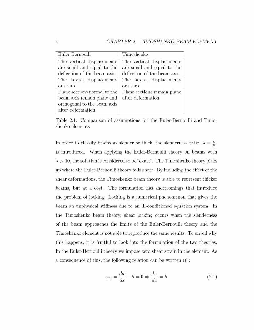
simplify the physics by assumptions. The assumptions are listed in Table
2.1[17].
The only difference in assumptions between the two theories is the last
one, as shear strain is included in the Timoshenko theory, the plane sections
are now no longer guaranteed to remain orthogonal to the beam axis after
deformation. Excluding shear strain is a valid assumption for slender beams.
3
4 CHAPTER 2. TIMOSHENKO BEAM ELEMENT
Euler-Bernoulli TimoshenkoThe vertical displacementsare small and equal to thedeflection of the beam axis
The vertical displacementsare small and equal to thedeflection of the beam axis
The lateral displacementsare zero
The lateral displacementsare zero
Plane sections normal to thebeam axis remain plane andorthogonal to the beam axisafter deformation
Plane sections remain planeafter deformation
Table 2.1: Comparison of assumptions for the Euler-Bernoulli and Timo-shenko elements
In order to classify beams as slender or thick, the slenderness ratio, λ = Lh,
is introduced. When applying the Euler-Bernoulli theory on beams with
λ > 10, the solution is considered to be “exact”. The Timoshenko theory picks
up where the Euler-Bernoulli theory falls short. By including the effect of the
shear deformations, the Timoshenko beam theory is able to represent thicker
beams, but at a cost. The formulation has shortcomings that introduce
the problem of locking. Locking is a numerical phenomenon that gives the
beam an unphysical stiffness due to an ill-conditioned equation system. In
the Timoshenko beam theory, shear locking occurs when the slenderness
of the beam approaches the limits of the Euler-Bernoulli theory and the
Timoshenko element is not able to reproduce the same results. To unveil why
this happens, it is fruitful to look into the formulation of the two theories.
In the Euler-Bernoulli theory we impose zero shear strain in the element. As
a consequence of this, the following relation can be written[18]:
γxz =dw
dx− θ = 0⇒ dw
dx= θ (2.1)
5
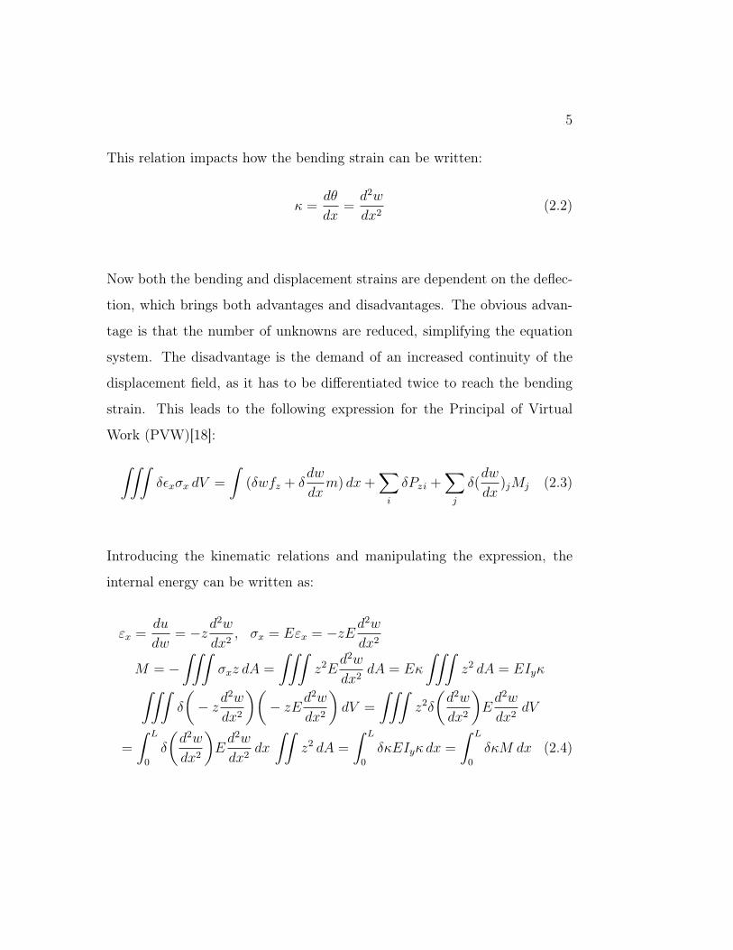
This relation impacts how the bending strain can be written:
κ =dθ
dx=d2w
dx2(2.2)
Now both the bending and displacement strains are dependent on the deflec-
tion, which brings both advantages and disadvantages. The obvious advan-
tage is that the number of unknowns are reduced, simplifying the equation
system. The disadvantage is the demand of an increased continuity of the
displacement field, as it has to be differentiated twice to reach the bending
strain. This leads to the following expression for the Principal of Virtual
Work (PVW)[18]:
∫∫∫δεxσx dV =
∫(δwfz + δ
dw
dxm) dx+
∑i
δPzi +∑j
δ(dw
dx)jMj (2.3)
Introducing the kinematic relations and manipulating the expression, the
internal energy can be written as:
εx =du
dw= −zd
2w
dx2, σx = Eεx = −zEd
2w
dx2
M = −∫∫∫
σxz dA =
∫∫∫z2E
d2w
dx2dA = Eκ
∫∫∫z2 dA = EIyκ∫∫∫
δ
(− zd
2w
dx2
)(− zEd
2w
dx2
)dV =
∫∫∫z2δ
(d2w
dx2
)Ed2w
dx2dV
=
∫ L
0
δ
(d2w
dx2
)Ed2w
dx2dx
∫∫z2 dA =
∫ L
0
δκEIyκ dx =
∫ L
0
δκM dx (2.4)
6 CHAPTER 2. TIMOSHENKO BEAM ELEMENT
In a Timoshenko beam element the same trick is not applicable as the shear
strain is now included. The rotation of the cross section can now be expressed
as:dwdx
+ φ = θ , with φ being the additional rotation of the cross section due
to shear. This changes the formulation of PVW[17]:
∫∫∫(δεxσx + δγxzτxz) dV =
∫ L
0
(δwfz + δθmdx+∑i
δwiPzi +∑j
δθjMj
(2.5)
This time the formulation contains two unknowns and another contribution
from the internal forces. This will in turn affect the stiffness matrix, which is
shown in Section 2.2. The internal energy can once again be rewritten when
the kinematic relations are included:
κ =dθ
dx, εx =
du
dx= −z dθ
dx, σx = Eεx = −zE dθ
dx(2.6)
γxz =dw
dx+du
dx=dw
dx− θ, τxz = Gγxz = G(
dw
dx− θ) (2.7)
M = −∫∫
σxz dA = Eκ
∫∫z2 dA = EIyκ (2.8)
Q =
∫∫τxz dA =
∫∫Gγxz dA =
E
2(1 + ν)(dw
dx−θ)
∫∫dA = GAγxz (2.9)
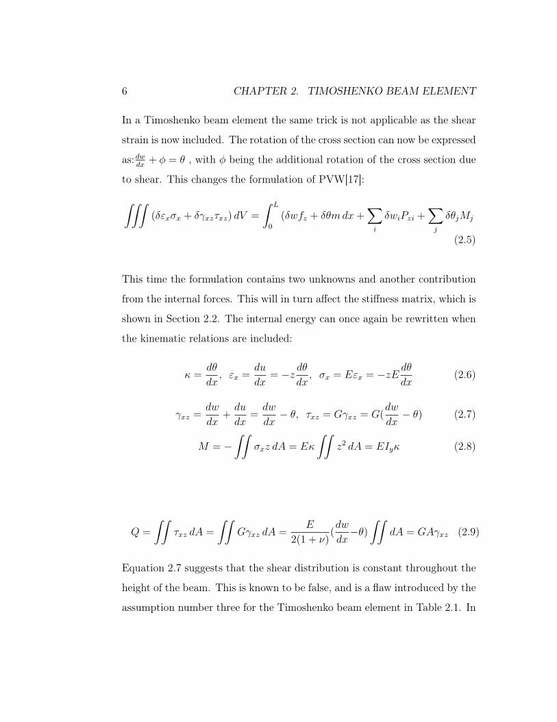
Equation 2.7 suggests that the shear distribution is constant throughout the
height of the beam. This is known to be false, and is a flaw introduced by the
assumption number three for the Timoshenko beam element in Table 2.1. In
7
reality the cross-section would not remain plane, but distorted as illustrated
in Figure 2.1:
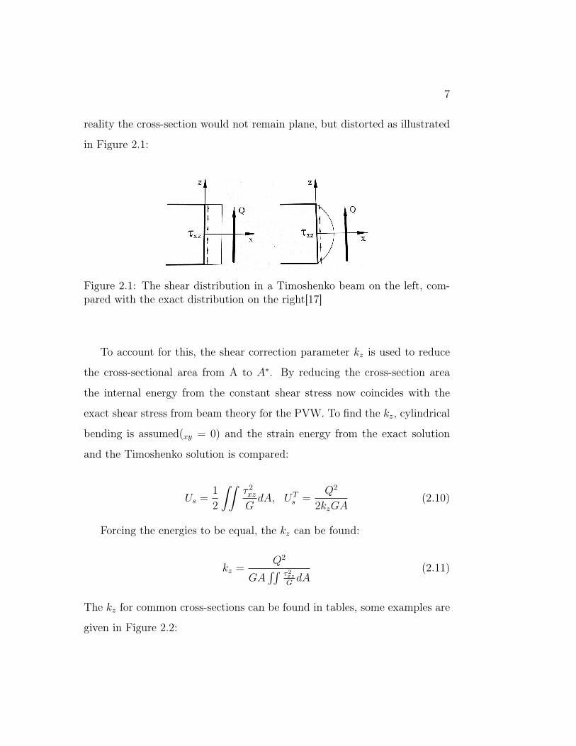
Figure 2.1: The shear distribution in a Timoshenko beam on the left, com-pared with the exact distribution on the right[17]
To account for this, the shear correction parameter kz is used to reduce
the cross-sectional area from A to A∗. By reducing the cross-section area
the internal energy from the constant shear stress now coincides with the
exact shear stress from beam theory for the PVW. To find the kz, cylindrical
bending is assumed(xy = 0) and the strain energy from the exact solution
and the Timoshenko solution is compared:
Us =1
2
∫∫τ 2xz
GdA, UT
s =Q2
2kzGA(2.10)
Forcing the energies to be equal, the kz can be found:
kz =Q2
GA∫∫ τ2xz
GdA
(2.11)
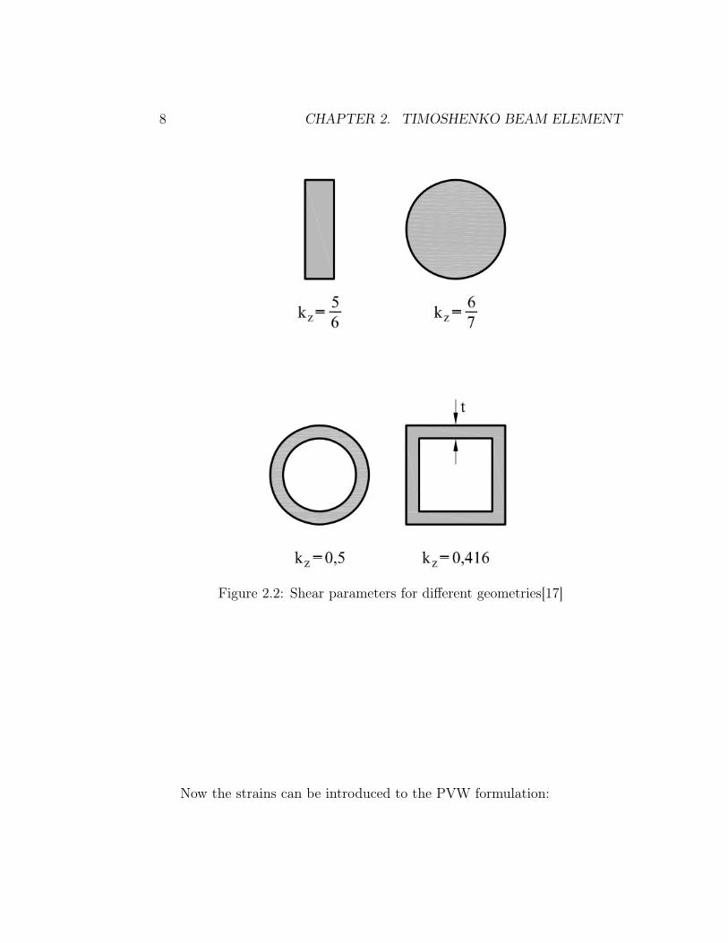
The kz for common cross-sections can be found in tables, some examples are
given in Figure 2.2:
8 CHAPTER 2. TIMOSHENKO BEAM ELEMENT
Figure 2.2: Shear parameters for different geometries[17]
Now the strains can be introduced to the PVW formulation:
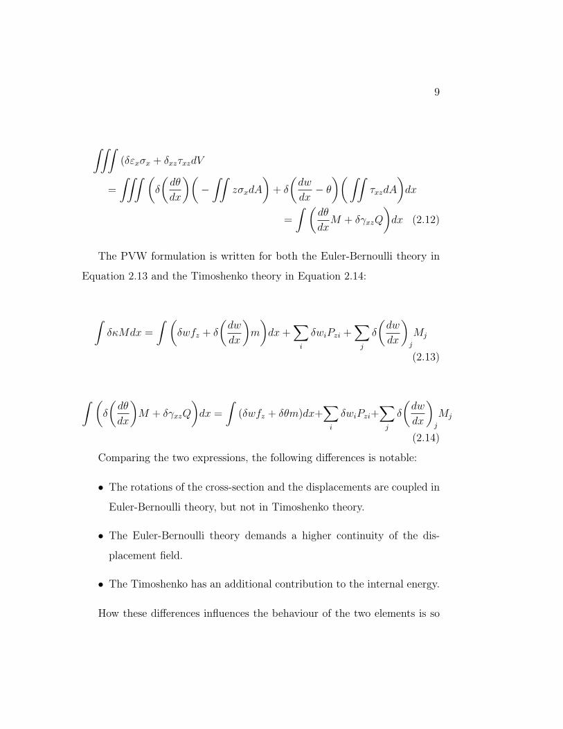
9
∫∫∫(δεxσx + δxzτxzdV
=
∫∫∫ (δ
(dθ
dx
)(−∫∫
zσxdA
)+ δ
(dw
dx− θ)(∫∫
τxzdA
)dx
=
∫ (dθ
dxM + δγxzQ
)dx (2.12)
The PVW formulation is written for both the Euler-Bernoulli theory in
Equation 2.13 and the Timoshenko theory in Equation 2.14:
∫δκMdx =
∫ (δwfz + δ
(dw
dx
)m
)dx+
∑i
δwiPzi +∑j
δ
(dw
dx
)j
Mj
(2.13)
∫ (δ
(dθ
dx
)M + δγxzQ
)dx =
∫(δwfz + δθm)dx+
∑i
δwiPzi+∑j
δ
(dw
dx
)j
Mj
(2.14)
Comparing the two expressions, the following differences is notable:
• The rotations of the cross-section and the displacements are coupled in
Euler-Bernoulli theory, but not in Timoshenko theory.
• The Euler-Bernoulli theory demands a higher continuity of the dis-
placement field.
• The Timoshenko has an additional contribution to the internal energy.
How these differences influences the behaviour of the two elements is so
10 CHAPTER 2. TIMOSHENKO BEAM ELEMENT
far not obvious, but will become clearer in the following sections when the
stiffness matrices are assembled.
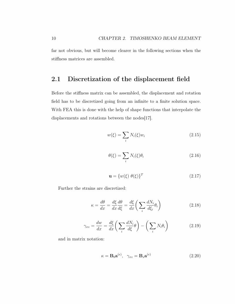
2.1 Discretization of the displacement field
Before the stiffness matrix can be assembled, the displacement and rotation
field has to be discretized going from an infinite to a finite solution space.
With FEA this is done with the help of shape functions that interpolate the
displacements and rotations between the nodes[17].
w(ξ) =∑i
Ni(ξ)wi (2.15)
θ(ξ) =∑i
Ni(ξ)θi (2.16)
u = {w(ξ) θ(ξ)}T (2.17)
Further the strains are discretized:
κ =dθ
dx=dξ
dx
dθ
dξ=dξ
dx
(∑i
dNi
dξiθi
)(2.18)
γxz =dw
dx=dξ
dx
(∑i
dNi
dξθ
)−(∑
i
Niθi
)(2.19)
and in matrix notation:
κ = Bba(e), γxz = Bsa(e) (2.20)
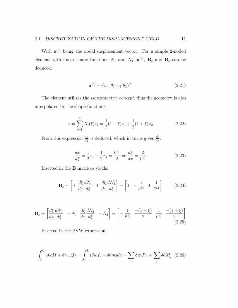
2.1. DISCRETIZATION OF THE DISPLACEMENT FIELD 11
With a(e) being the nodal displacement vector. For a simple 2-noded
element with linear shape functions N1 and N2, a(e), Bs and Bb can be
deduced:
a(e) = {w1 θ1 w2 θ2}T (2.21)
The element utilizes the isoparametric concept, thus the geometry is also
interpolated by the shape functions:
x =2∑i=1
Ni(ξ)xi =1
2(1− ξ)x1 +
1
2(1 + ξ)x2 (2.22)
From this expression dxdξ
is deduced, which in turns gives dξdx:
dx
dξ=
1
2x1 +
1
2x2 =
l(e)
2⇒ dξ
dx=
2
l(e)(2.23)
Inserted in the B matrices yields:
Bs =
[0
dξ
dx
dN1
dξ0
dξ
dx
dN2
dξ
]=
[0 − 1
l(e)0
1
l(e)
](2.24)
Bs =
[dξ
dx
dN1
dξ−N1
dξ
dx
dN2
dξ−N2
]=
[− 1
l(e)−(1− ξ)
2
1
l(e)−(1 + ξ)
2
](2.25)
Inserted in the PVW expression:
∫ L
0
(δκM + δγxzQ) =
∫ L
0
(δwfz + δθm)dx+∑i
δwiPzi +∑j
δθMj (2.26)
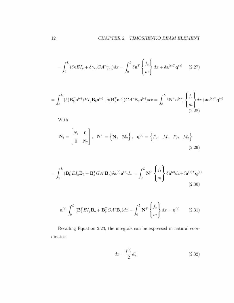
12 CHAPTER 2. TIMOSHENKO BEAM ELEMENT
=
∫ L
0
(δκEIy + δγxzGA∗γxz)dx =
∫ L
0
δuT
fzm dx+ δa(e)Tq(e) (2.27)
=
∫ L
0
(δ(BTb a
(e))EIyBba(e)+δ(BTs a
(e))GA∗Bsa(e))dx =
∫ L
0
δNTa(e))
fzmdx+δa(e)Tq(e)
(2.28)
With
Ni =
N1 0
0 N2
, NT ={N1 N2
}, q(e) =
{Fz1 M1 Fz2 M2
}(2.29)
=
∫ L
0
(BTb EIyBb + BT
sGA∗Bs)δa(e)a(e)dx =
∫ L
0
NT
fzm δa(e)dx+δa(e)Tq(e)
(2.30)
a(e)
∫ L
0
(BTb EIyBb + BT
sGA∗Bs)dx−
∫ L
0
NT
fzm dx = q(e) (2.31)
Recalling Equation 2.23, the integrals can be expressed in natural coor-
dinates:
dx =l(e)
2dξ (2.32)
2.1. DISCRETIZATION OF THE DISPLACEMENT FIELD 13
:
Kb =
∫ 1
−1
BTb EIyBbdξ (2.33)
Ks =
∫ 1
−1
BTsGA
∗Bsdξ (2.34)
f(e) =
∫ 1
−1
NT
fzm l(e)
2dξ (2.35)
For uniformly distributed values of fz and m the equivalent nodal force
vector, f(e), can be simplified:
f(e) =
f(e)1
f(e)2
, f(e)i =
l(e)
2
fzm∫ 1
−1
Nidξ =l(e)
2
fzm (2.36)
f1 = f2 ==l(e)
2
fzm (2.37)
i.e. the total distributed vertical forces and moments are split equally be-
tween the two nodes[17]. Note that in contrast to the Euler-Bernoulli theory,
the distributed forces are independent of the distributed moments. This is
due to the independent interpolation of the rotation and deflection, and as
a consequence of this, the demand of continuity for the interpolation is only
C0. The integration is undertaking using the Gaussian quadrature rule:
K(e) =
np∑p=1
BTb EIyBbWp
l(e)
2+
np∑p=1
BTsGA
∗BsWpl(e)
2(2.38)
14 CHAPTER 2. TIMOSHENKO BEAM ELEMENT
As mentioned earlier, splitting the element stiffness matrix into a bending
and shear part can be more convenient. This makes it easier to identify the
contributions from the different forces and makes it easier to apply a different
order of integration to the different contributions. The latter can be useful
when trying to abolish the defect from shear locking. This will be elaborated
in the following section.
2.2 Shear locking
In order to illustrate the effect of shear locking, a cantilever beam with a
concentrated load applied at the free end is modelled with both the Euler-
Bernoulli and the Timoshenko theory. For simplicity, the beam is approxi-
mated with only one element. In this example the element stiffness matrix
will be assembled separately for bending and shear. First the bending stiff-
ness is assembled:
K(e)b = EIy
l(e)
2
∫ 1
−1
BTb Bbdξ (2.39)
K(e)b = EIy
l(e)
2
∫ 1
−1
[0 − 1
l(e)0
1
l(e)
]T[0 − 1
l(e)0
1
l(e)
]dξ (2.40)
As the beam consists of one element l(e) = L, and the matrix only contain
constants, Kb can be integrated using only one Gauss point, yielding[]:
2.2. SHEAR LOCKING 15
Kb =EIy2L
0 0 0 0
0 1 0 −1
0 0 0 0
0 −1 0 1
(2.41)
Moving on to the Ks:
Ks = GA∗L
2
∫ 1
−1
[− 1
l(e)−(1− ξ)
2
1
l(e)−(1 + ξ)
2
]T[− 1
l(e)−(1− ξ)
2
1
l(e)−(1 + ξ)
2
]dξ
(2.42)
Ks consists of quadratic terms of ξ, and in order to achieve exact inte-
gration two Gauss quadrature points have to be used, yielding:
Ks =GA∗
L
1L
12− 1L
12
12
L3−1
2L6
− 1L−1
21L−1
2
12
L6−1
2L3
(2.43)
Combining the two matrices and eliminating the clamped degrees of free-
dom yields:
Kb =
0 0
0 EIyL
(2.44)
Ks =
GA∗
L−GA∗
2
−GA∗
2GA∗
3L
(2.45)
16 CHAPTER 2. TIMOSHENKO BEAM ELEMENT
Kb + Ks =
GA∗
L−GA∗
2
−GA∗
2
(GA∗
3L+ EIy
L
) (2.46)
This combined matrix can be compared with the matrix deduced with
the Euler-Bernoulli theory[18]:
KEB =
12EIyL3 −6EIy
L2
−6EIyL2
4EIyL
(2.47)
The Timoshenko element is expected to give the same results as the
Euler-Bernoulli element for slender beams. To investigate this, the can-
tilever problem is solved using both elements with P = 1, starting with the
Euler-Bernoulli element:
12EIyL3 −6EIy
L2
−6EIyL2
4EIyL
w2
θ2
=
1
0
(2.48)
w2
θ2
=
L3
3EIyL2
2EIy
L2
2EIyLEIy
1
0
(2.49)
wEB2 =L3
3EIy, θEB2 =
L2
2EIy(2.50)
GA∗
L−GA∗
2
−GA∗
2
(GA∗
3L+ EIy
L
)w2
θ2
=
1
0
(2.51)
β =12EIyL2GA∗
=E
Gkzλ2(2.52)

2.2. SHEAR LOCKING 17
w2
θ2
=β
β + 1
(
LGA∗ + L3
3EIy
)L2
2EIy
L2
2EIyLEIy
1
0
[17] (2.53)
wT2 =β
β + 1
(L
GA∗+
L3
3EIy
), θT2 =
β
β + 1
L2
2EIy(2.54)
As the slenderness of the beam increases, the solution from the Timo-
shenko element should approach the one obtained from the Euler-Bernoulli
element:
rw =wT2EB2
=β
β + 1
( LGA∗ + L3
EIy
L3
3EIy
)=
3(4λ2 + 3)
4λ2(λ2 + 3)(2.55)
limλ→∞
3(4λ2 + 3)
4λ2(λ2 + 3)= 0 (2.56)
[17]
Equation 2.56 shows that instead of converging towards the Euler-Bernoulli
solution, the solution from the Timoshenko element becomes progressively
stiffer as the slenderness increases. This is due to the phenomena of shear
locking. Numerous methods have been developed to eliminate this defect
from the Timoshenko beam element. In this paper the method of reduced in-
tegration and residual bending flexibility (RBF) is elaborated in the following
sections.
18 CHAPTER 2. TIMOSHENKO BEAM ELEMENT
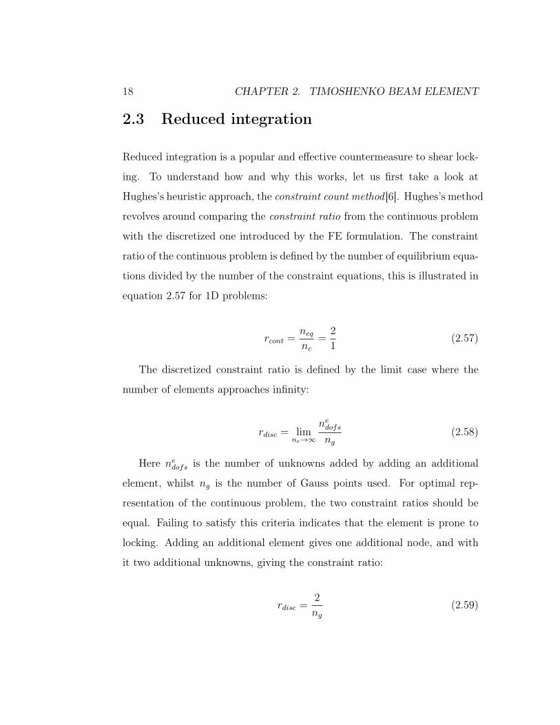
2.3 Reduced integration
Reduced integration is a popular and effective countermeasure to shear lock-
ing. To understand how and why this works, let us first take a look at
Hughes’s heuristic approach, the constraint count method [6]. Hughes’s method
revolves around comparing the constraint ratio from the continuous problem
with the discretized one introduced by the FE formulation. The constraint
ratio of the continuous problem is defined by the number of equilibrium equa-
tions divided by the number of the constraint equations, this is illustrated in
equation 2.57 for 1D problems:
rcont =neqnc
=2
1(2.57)
The discretized constraint ratio is defined by the limit case where the
number of elements approaches infinity:
rdisc = limne→∞
nedofsng
(2.58)
Here nedofs is the number of unknowns added by adding an additional
element, whilst ng is the number of Gauss points used. For optimal rep-
resentation of the continuous problem, the two constraint ratios should be
equal. Failing to satisfy this criteria indicates that the element is prone to
locking. Adding an additional element gives one additional node, and with
it two additional unknowns, giving the constraint ratio:
rdisc =2
ng(2.59)
2.4. RESIDUAL BENDING FLEXIBILITY, RBF 19
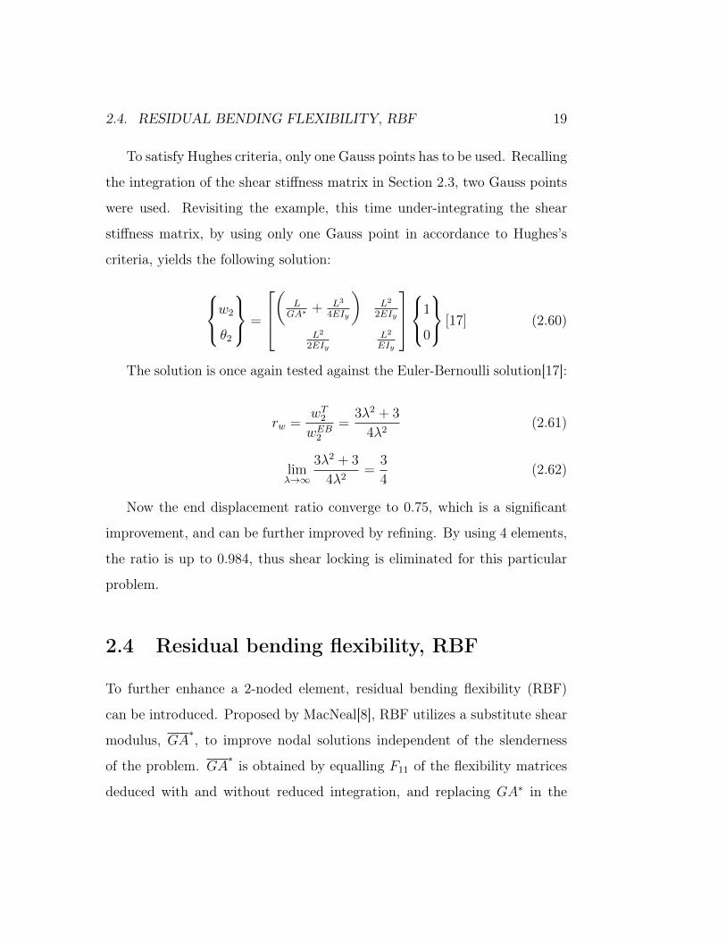
To satisfy Hughes criteria, only one Gauss points has to be used. Recalling
the integration of the shear stiffness matrix in Section 2.3, two Gauss points
were used. Revisiting the example, this time under-integrating the shear
stiffness matrix, by using only one Gauss point in accordance to Hughes’s
criteria, yields the following solution:
w2
θ2
=
(
LGA∗ + L3
4EIy
)L2
2EIy
L2
2EIyL2
EIy
1
0
[17] (2.60)
The solution is once again tested against the Euler-Bernoulli solution[17]:
rw =wT2wEB2
=3λ2 + 3
4λ2(2.61)
limλ→∞
3λ2 + 3
4λ2=
3
4(2.62)
Now the end displacement ratio converge to 0.75, which is a significant
improvement, and can be further improved by refining. By using 4 elements,
the ratio is up to 0.984, thus shear locking is eliminated for this particular
problem.
2.4 Residual bending flexibility, RBF
To further enhance a 2-noded element, residual bending flexibility (RBF)
can be introduced. Proposed by MacNeal[8], RBF utilizes a substitute shear
modulus, GA∗, to improve nodal solutions independent of the slenderness
of the problem. GA∗ is obtained by equalling F11 of the flexibility matrices
deduced with and without reduced integration, and replacing GA∗ in the
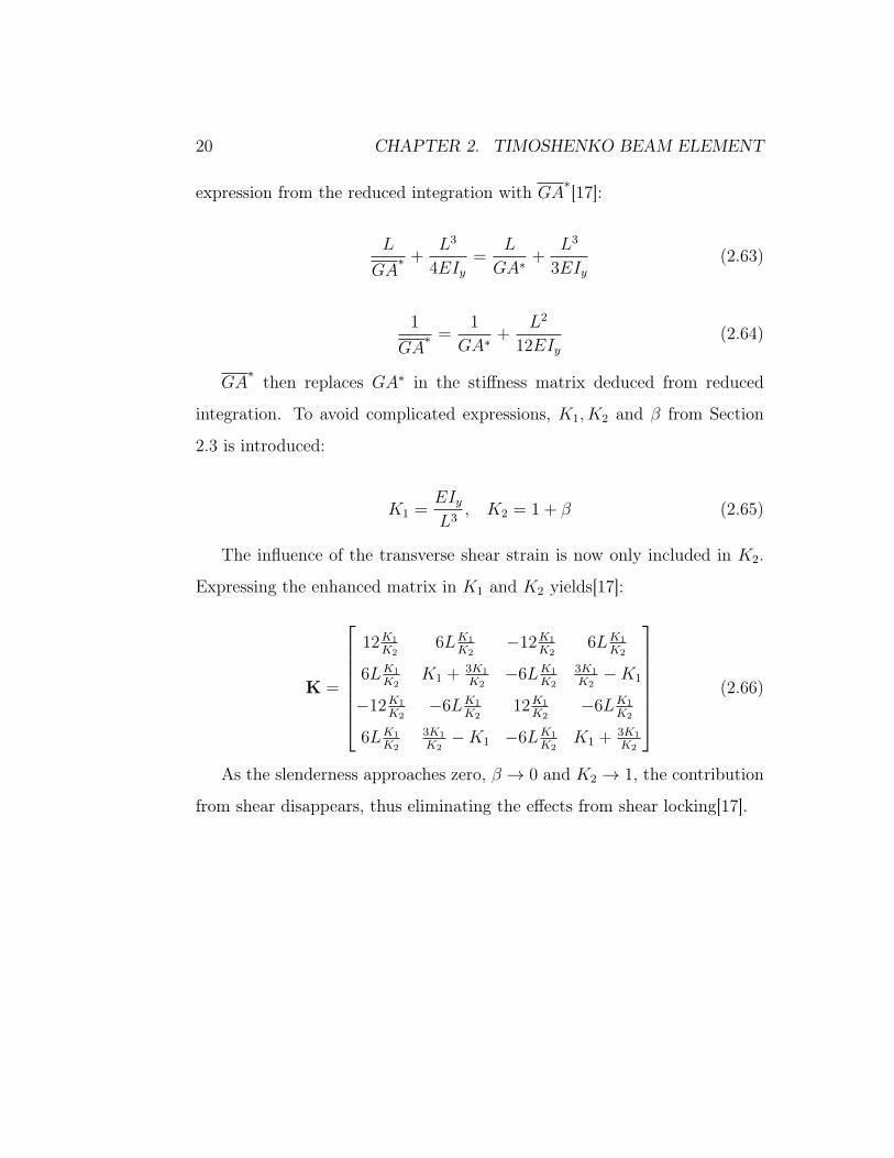
20 CHAPTER 2. TIMOSHENKO BEAM ELEMENT
expression from the reduced integration with GA∗[17]:
L
GA∗ +
L3
4EIy=
L
GA∗+
L3
3EIy(2.63)
1
GA∗ =
1
GA∗+
L2
12EIy(2.64)
GA∗ then replaces GA∗ in the stiffness matrix deduced from reduced
integration. To avoid complicated expressions, K1, K2 and β from Section
2.3 is introduced:
K1 =EIyL3
, K2 = 1 + β (2.65)
The influence of the transverse shear strain is now only included in K2.
Expressing the enhanced matrix in K1 and K2 yields[17]:
K =
12K1
K26LK1
K2−12K1
K26LK1
K2
6LK1
K2K1 + 3K1
K2−6LK1
K2
3K1
K2−K1
−12K1
K2−6LK1
K212K1
K2−6LK1
K2
6LK1
K2
3K1
K2−K1 −6LK1
K2K1 + 3K1
K2
(2.66)
As the slenderness approaches zero, β → 0 and K2 → 1, the contribution
from shear disappears, thus eliminating the effects from shear locking[17].
Chapter 3
Nonlinear Equilibrium Equations
In Finite Element Analysis (FEA), the response of the structure is expected
to be linear. However, for many problems this is not the case. For structural
problems, the nonlinearities can come from several sources, such as geometric
nonlinearity, material nonlinearity, load nonlinearity and boundary condition
nonlinearity. The physical source of geometric nonlinearity emerges when the
change in geometry from the structure deforming, affects the kinematic and
equilibrium equations. This can occur for slender structures, stability prob-
lems or tensile structures, such as cables or inflatable membranes[12]. This
leads to a nonlinear strain-displacement operator, [∂], now being dependent
on the displacements, u[12]:
{ε} = [∂]{u} (3.1)
This in turns effect the relation between strains and stresses, as the trans-
posed strain-displacement operator is no longer guaranteed to be equal to the
operator applied to the stresses.
21
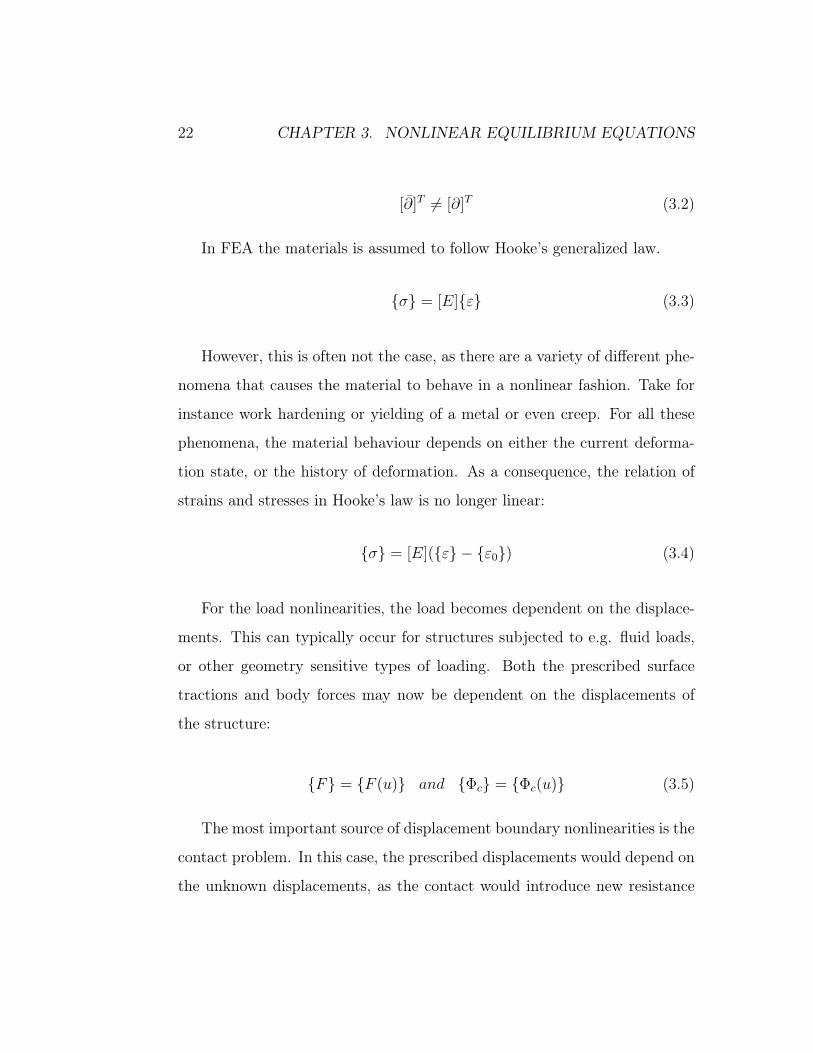
22 CHAPTER 3. NONLINEAR EQUILIBRIUM EQUATIONS
[∂]T 6= [∂]T (3.2)
In FEA the materials is assumed to follow Hooke’s generalized law.
{σ} = [E]{ε} (3.3)
However, this is often not the case, as there are a variety of different phe-
nomena that causes the material to behave in a nonlinear fashion. Take for
instance work hardening or yielding of a metal or even creep. For all these
phenomena, the material behaviour depends on either the current deforma-
tion state, or the history of deformation. As a consequence, the relation of
strains and stresses in Hooke’s law is no longer linear:
{σ} = [E]({ε} − {ε0}) (3.4)
For the load nonlinearities, the load becomes dependent on the displace-
ments. This can typically occur for structures subjected to e.g. fluid loads,
or other geometry sensitive types of loading. Both the prescribed surface
tractions and body forces may now be dependent on the displacements of
the structure:
{F} = {F (u)} and {Φc} = {Φc(u)} (3.5)
The most important source of displacement boundary nonlinearities is the
contact problem. In this case, the prescribed displacements would depend on
the unknown displacements, as the contact would introduce new resistance
3.1. SOLVING NONLINEAR EQUILIBRIUM EQUATIONS 23
to the structure. The prescribed displacements now become a function of the
unknown ones:
{uc} = {uc(u)} (3.6)
Common for all of these cases, is that the linear relation between loads and
displacements can no longer be used, so the nonlinear relation is introduced,
were both the stiffness and the load becomes functions of the displacements:
[K(u)]{u} = {R(u)} (3.7)
3.1 Solving Nonlinear Equilibrium Equations
To solve the nonlinear force-displacement relation presented in the previous
section, an iterative approach is developed. The first step is to "guess" a
displacement, called the predictor step. To evaluate how good the initial
guess, u1, has been, the residual force, Rres, is introduced. The residual force
represents the out of balance forces, by comparing the external and internal
forces in the structure.
{Rext} − {Rint} = {Rres} (3.8)
By doing a Taylor series expansion of the residual force at the state of
u1, and neglecting the higher order terms, yields the incremental equilibrium
equation[12]:
24 CHAPTER 3. NONLINEAR EQUILIBRIUM EQUATIONS
R(u) ∼= R1 +
(dR1
du
)(u− u1) = 0 (3.9)
The gradient of the incremental equilibrium equation is called the tangent
stiffness matrix, KT , and by taking the inverse of KT , yields an expression
for ∆u, and further a new approximation for the displacement:
∆u1 = −(dR1
du
)−1
R1, u2 = u1 + ∆u1 (3.10)
Then a new and hopefully smaller residual force is calculated, using
the new approximation. This procedure is repeated until the residual force
reaches a prescribed tolerance[14]:
Rres ≤ Rtol (3.11)
This is called a Newton-Raphson iteration. Combining this with a forward
Euler load incrementation, is one of the most common and simplest methods
to solve the nonlinear equations. For the full Newton-Raphson, the load is
applied in increments and the convergence for each increment is obtained
before proceeding to the next. This is illustrated in with an algorithm in
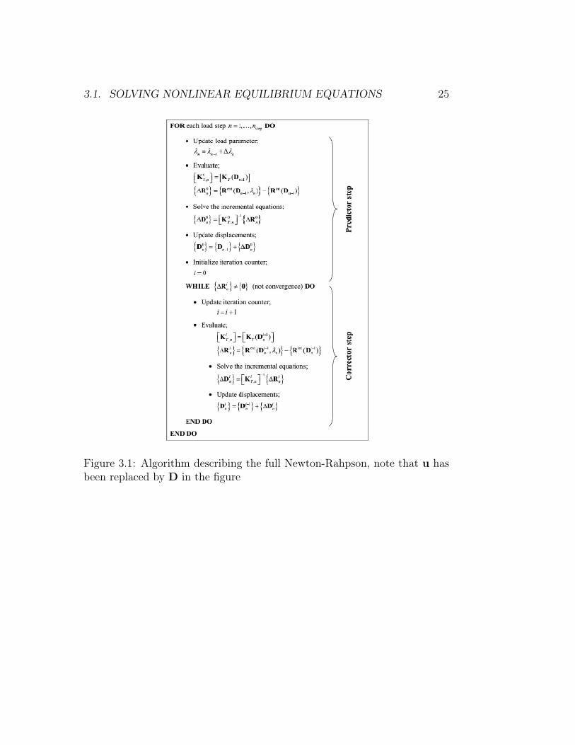
Figure 3.1[14]:
If the tangent stiffness, KT , is calculated for every step, the method
is classified as a full or true Newton-Rahpson. Although this is a reliable
method for many problems, the majority of computational time is spent
updating the KT . To reduce the computational effort, several methods have
been proposed, modifying the full Newton-Raphson, but they will not be
elaborated in this paper.
3.1. SOLVING NONLINEAR EQUILIBRIUM EQUATIONS 25
Figure 3.1: Algorithm describing the full Newton-Rahpson, note that u hasbeen replaced by D in the figure
26 CHAPTER 3. NONLINEAR EQUILIBRIUM EQUATIONS
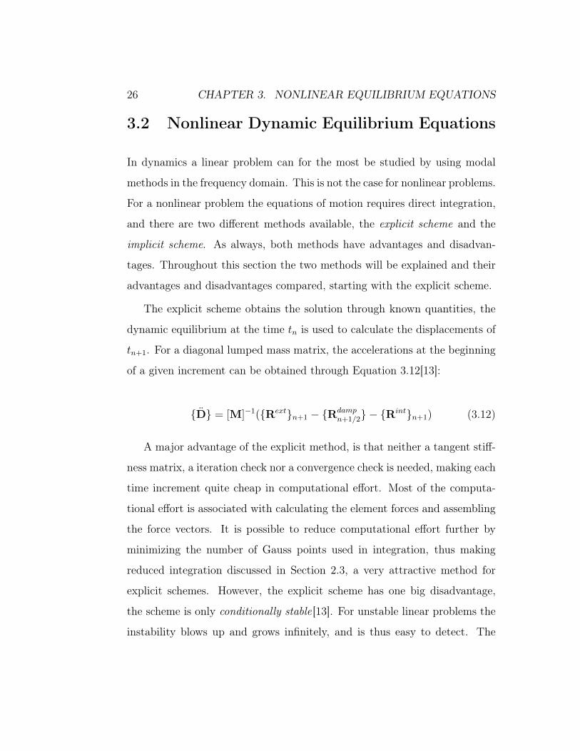
3.2 Nonlinear Dynamic Equilibrium Equations
In dynamics a linear problem can for the most be studied by using modal
methods in the frequency domain. This is not the case for nonlinear problems.
For a nonlinear problem the equations of motion requires direct integration,
and there are two different methods available, the explicit scheme and the
implicit scheme. As always, both methods have advantages and disadvan-
tages. Throughout this section the two methods will be explained and their
advantages and disadvantages compared, starting with the explicit scheme.
The explicit scheme obtains the solution through known quantities, the
dynamic equilibrium at the time tn is used to calculate the displacements of
tn+1. For a diagonal lumped mass matrix, the accelerations at the beginning
of a given increment can be obtained through Equation 3.12[13]:
{D} = [M]−1({Rext}n+1 − {Rdampn+1/2} − {R
int}n+1) (3.12)
A major advantage of the explicit method, is that neither a tangent stiff-
ness matrix, a iteration check nor a convergence check is needed, making each
time increment quite cheap in computational effort. Most of the computa-
tional effort is associated with calculating the element forces and assembling
the force vectors. It is possible to reduce computational effort further by
minimizing the number of Gauss points used in integration, thus making
reduced integration discussed in Section 2.3, a very attractive method for
explicit schemes. However, the explicit scheme has one big disadvantage,
the scheme is only conditionally stable[13]. For unstable linear problems the
instability blows up and grows infinitely, and is thus easy to detect. The

3.2. NONLINEAR DYNAMIC EQUILIBRIUM EQUATIONS 27
nonlinear instability on the other hand, can be much harder to detect, as
the artificially introduced energy can be dissipated by e.g. elastic-plastic
material behaviour, making it an even worse attribute[13]. For the explicit
scheme the time step, ∆t has to be less than the stable time increment ∆tcr.
∆tcr can be found by looking at the eigenfrequencies, ωj, and the fraction of
critical damping, ξj. Assuming that the damping is small for all modes, ∆tcr
can be found for the highest natural frequency[13]:
∆tcr ≤2
ωmax(√
1− ξ2 − ξ) (3.13)
For a system without damping, ∆tcr can be found by:
∆tcr ≤2
ωmax(3.14)
∆tcr can also be expressed in the minimum time it takes a dilatational
wave to travel across the smallest element in the model[13]:
∆tcr =l(e)
cd, with cd =
√E
ρ(3.15)
Note that the material properties that effect ∆tcr, are the instantaneous
values.
Summing up the explicit scheme, it is a simple method with low compu-
tational cost for each time step, but it needs a very small time step in order
to remain stable. To check whether the scheme is stable, an energy balance
for the model can be evaluated.
In contrast to the explicit scheme, the implicit scheme requires solving of
the nonlinear algebraic equations for every time step. The scheme also needs
28 CHAPTER 3. NONLINEAR EQUILIBRIUM EQUATIONS
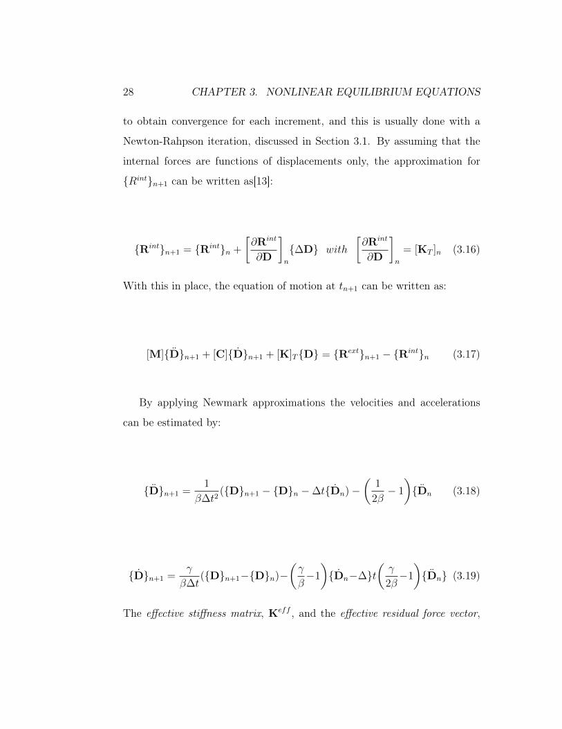
to obtain convergence for each increment, and this is usually done with a
Newton-Rahpson iteration, discussed in Section 3.1. By assuming that the
internal forces are functions of displacements only, the approximation for
{Rint}n+1 can be written as[13]:
{Rint}n+1 = {Rint}n +
[∂Rint
∂D
]n
{∆D} with
[∂Rint
∂D
]n
= [KT ]n (3.16)
With this in place, the equation of motion at tn+1 can be written as:
[M]{D}n+1 + [C]{D}n+1 + [K]T{D} = {Rext}n+1 − {Rint}n (3.17)
By applying Newmark approximations the velocities and accelerations
can be estimated by:
{D}n+1 =1
β∆t2({D}n+1 − {D}n −∆t{Dn)−
(1
2β− 1
){Dn (3.18)
{D}n+1 =γ
β∆t({D}n+1−{D}n)−
(γ
β−1
){Dn−∆}t
(γ
2β−1
){Dn} (3.19)
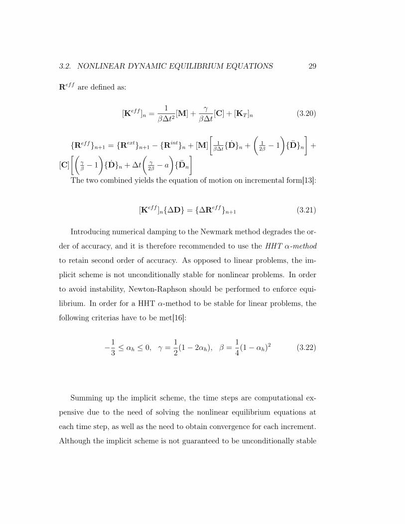
The effective stiffness matrix, Keff , and the effective residual force vector,
3.2. NONLINEAR DYNAMIC EQUILIBRIUM EQUATIONS 29
Reff are defined as:
[Keff ]n =1
β∆t2[M] +
γ
β∆t[C] + [KT ]n (3.20)
{Reff}n+1 = {Rext}n+1 − {Rint}n + [M]
[1β∆t{D}n +
(1
2β− 1
){D}n
]+
[C]
[(γβ− 1
){D}n + ∆t
(γ2β− a){Dn
]The two combined yields the equation of motion on incremental form[13]:
[Keff ]n{∆D} = {∆Reff}n+1 (3.21)
Introducing numerical damping to the Newmark method degrades the or-
der of accuracy, and it is therefore recommended to use the HHT α-method
to retain second order of accuracy. As opposed to linear problems, the im-
plicit scheme is not unconditionally stable for nonlinear problems. In order
to avoid instability, Newton-Raphson should be performed to enforce equi-
librium. In order for a HHT α-method to be stable for linear problems, the
following criterias have to be met[16]:
−1
3≤ αh ≤ 0, γ =
1
2(1− 2αh), β =
1
4(1− αh)2 (3.22)
Summing up the implicit scheme, the time steps are computational ex-
pensive due to the need of solving the nonlinear equilibrium equations at
each time step, as well as the need to obtain convergence for each increment.
Although the implicit scheme is not guaranteed to be unconditionally stable

30 CHAPTER 3. NONLINEAR EQUILIBRIUM EQUATIONS
for nonlinear problems, it can run with a much bigger time step than the
explicit scheme.

3.3. STRAIN MEASURES FOR LARGE DEFORMATIONS 31
3.3 Strain measures for large deformations
To be able to compare the two FEA formulations applied in Chapter 4, it
is important to look into the strain measures the formulations utilizes. The
Green-Lagrange strain measure used by Abaqus, and the Biot strain measure,
utilized by the geometrically exact element used in Chapter 4.
To represent large deformations, the displacement vector u is introduced.
The displacement vector is defined by taking the position vector of the de-
formed configuration, x, and subtracting the position vector from the refer-
ence configuration, X[19].
u = x−X (3.23)
This is illustrated in Figure 3.2
Figure 3.2: Geometry description for large deformations in a Cartesian co-ordinate system[19]
In order to apply a mapping between a differential line element in the ref-
erence configuration to the deformed configuration, the deformation gradient,
F, is introduced:

32 CHAPTER 3. NONLINEAR EQUILIBRIUM EQUATIONS
dx = FdX (3.24)
F is defined by the base vectors, and can be used to map between
them[19]:
F = gi ⊗Gi, FT = Gi ⊗ gi, F−1 = Gi ⊗ gi, F−T = gi ⊗Gi (3.25)
Further the F is used to find the Green-Lagrange strain tensor, E.
E =1
2(FTF− I) (3.26)
I is the identity tensor, and by using the relations from Equation 3.25,
the Green-Lagrange tensor can be rewritten:
E =1
2((Gi ⊗ gi)(gj ⊗Gj)−GijGi ⊗Gj) =
1
2(gij −Gij)Gi ⊗Gj (3.27)
E = EijGi ⊗Gj (3.28)
Eij is the Green-Lagrange coefficients and is obtained through the metric
coefficients, gij and Gij, who determines the length and angle between the
base vectors[19]. The Green-Lagrange strain measure describes a nonlinear
relation between the displacements and strains, and is well suited to measure
strains under large deformations.
3.3. STRAIN MEASURES FOR LARGE DEFORMATIONS 33
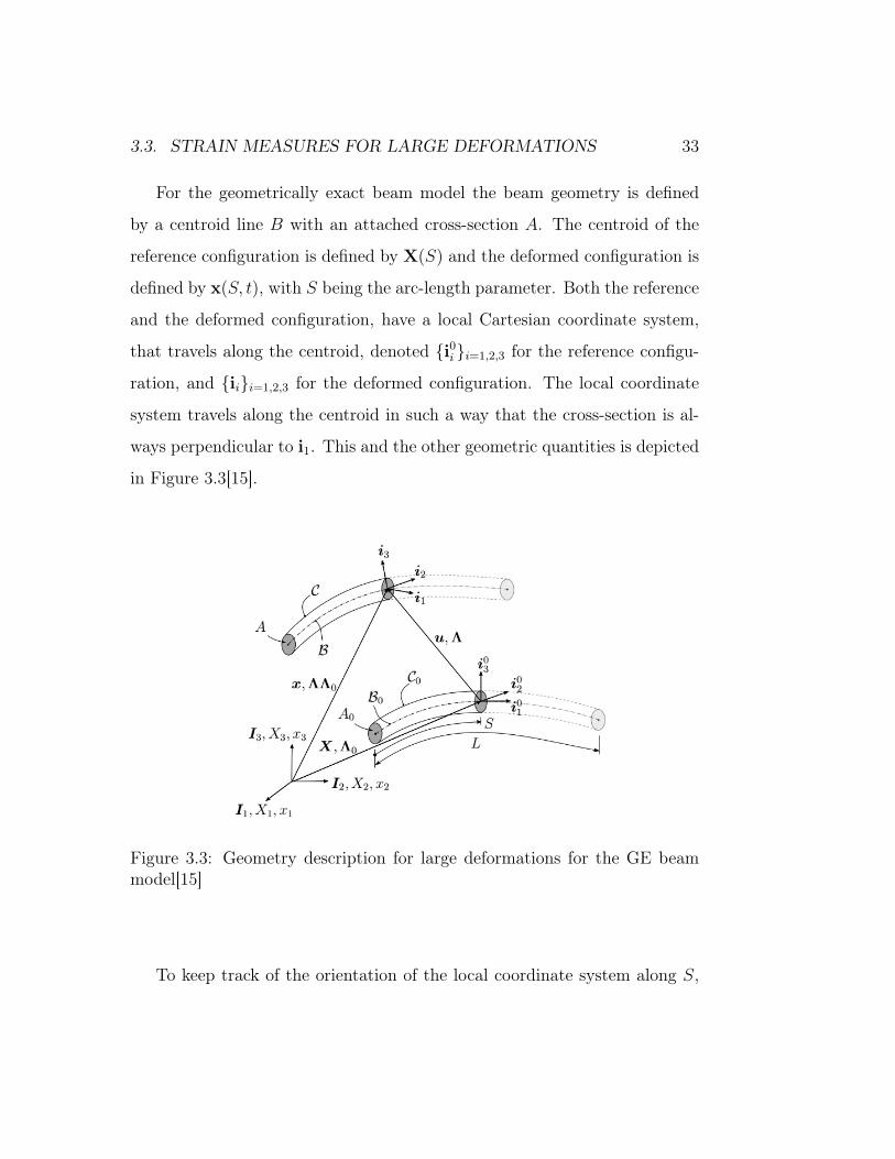
For the geometrically exact beam model the beam geometry is defined
by a centroid line B with an attached cross-section A. The centroid of the
reference configuration is defined by X(S) and the deformed configuration is
defined by x(S, t), with S being the arc-length parameter. Both the reference
and the deformed configuration, have a local Cartesian coordinate system,
that travels along the centroid, denoted {i0i }i=1,2,3 for the reference configu-
ration, and {ii}i=1,2,3 for the deformed configuration. The local coordinate
system travels along the centroid in such a way that the cross-section is al-
ways perpendicular to i1. This and the other geometric quantities is depicted
in Figure 3.3[15].
Figure 3.3: Geometry description for large deformations for the GE beammodel[15]
To keep track of the orientation of the local coordinate system along S,
34 CHAPTER 3. NONLINEAR EQUILIBRIUM EQUATIONS
the two-point tensor Λ(S, t) is defined, such that[15]:
ii(S, t) = Λ(S, t)i0i (S)⇒ Λ(S, t) = ii ⊗ i0i (3.29)
||ii|| = ||i0i || = 1 (3.30)
ΛTΛ = I (3.31)
Defining the reference and deformed configuration with respect to the
Cartesian frame Ii, the transformation gives:
ii(S, t) = Λ(S, t)Λ0(S)Ii ⇒ Λ0(S) = i0i ⊗ Ii (3.32)
The deformed configuration, C may now be uniquely determined, by the
deformed position and the rotation of the centroid[15].
C = {ϕ = (x,Λ) : [0, L]× [0, T ]→ R3 × SO(3)} (3.33)
SO(3) represents the group of all rotations about the origin of R3 under
the operation of composition. This means that the kinematics of the beam,
is reduced to a 1D description, with only the arc length coordinate, S, as a
parameter. The 3D beam geometry can now be defined by:
x3D(S, x0α, t) = x(S, t) + p(S, x0
α, t) = x(S, t) + Λ(S, t)x0αi
0α(S) (3.34)
3.3. STRAIN MEASURES FOR LARGE DEFORMATIONS 35
Where p(S, x0α) is the position vector of a point of the geometry, and
α denotes the two directions parallel to the cross-section. With x3D the
deformation gradient, F can be found:
F =∂x3D
∂x0i
⊗ i01 = (x′ + Λ′x0αi
0α)⊗ i01 + iα ⊗ i0α (3.35)
Due to the parameterization of the rotations[15], Λ′ can be expressed by
a skew symmetric-tensor, κ:
Λ′ = κΛ⇔ κ = Λ′ΛT (3.36)
By inserting κ and by adding and subtracting i1⊗i0i , the F can be written
with a polar material decomposition:
F = Λ{I + [ΛT (x′ − i1) + ΛT κx0αi
0α]⊗ i01} = ΛU (3.37)
With U being the right (current local) stretch tensor, that the Biot strain
measure can be derived from. The Biot strains are objective corotated engi-
neering strains that are independent of rigid body motions. The Biot strain
measure can be written as:
B = ΛTF− I = U− I = ε⊗ i1 (3.38)
ε = ΛT (γ + κp) (3.39)
With ε representing a generalized convected strain measure.
36 CHAPTER 3. NONLINEAR EQUILIBRIUM EQUATIONS
For interested readers the theory of the geometrically exact beam element
is further elaborated in A Comparative Study of Beam Element Formulations
for Nonlinear Analysis: Corotational vs Geometrically Exact Formulations,
Kjell M. Mathisen et al.[15]
Chapter 4
Numeric results
Throughout this chapter a number of different cantilever problems will be
solved using IFEM, an in-house software developed at SINTEF ICT, where
geometrically exact elements are implemented, and ABAQUS. Through these
tests, it is possible to study the convergence and accuracy of the elements and
compare them. All of the examples undertaken in this chapter are various
forms of slender cantilever beams, clamped at one end and loaded at the
other. The examples induce bending and displacements in more than one
direction, and to compare the results, the norm of displacement for both
the solution and its corresponding reference solution has been used. The
reference solution is found for each element by solving the problem with a
very fine grid.
u =√u2x + u2
y + u2z, uref =
√u2x,ref + u2
y,ref + u2z,ref
(4.1)
37
38 CHAPTER 4. NUMERIC RESULTS
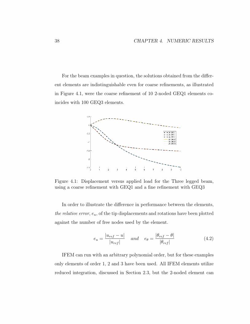
For the beam examples in question, the solutions obtained from the differ-
ent elements are indistinguishable even for coarse refinements, as illustrated
in Figure 4.1, were the coarse refinement of 10 2-noded GEQ1 elements co-
incides with 100 GEQ3 elements.
Figure 4.1: Displacement versus applied load for the Three legged beam,using a coarse refinement with GEQ1 and a fine refinement with GEQ3
In order to illustrate the difference in performance between the elements,
the relative error, eu, of the tip displacements and rotations have been plotted
against the number of free nodes used by the element.
eu =|uref − u||uref |
and eθ =|θref − θ||θref |
(4.2)
IFEM can run with an arbitrary polynomial order, but for these examples
only elements of order 1, 2 and 3 have been used. All IFEM elements utilize
reduced integration, discussed in Section 2.3, but the 2-noded element can
39
also be run with a RBF formulation, discussed in Section 2.4. IFEM will
be compared with the shear flexible beam elements from ABAQUS, B31 and
B32. One important difference between the ABAQUS and IFEM is the strain
measure they utilize. IFEM utilizes the Biot strain measure, whilst ABAQUS
utilizes the Green-Lagrange strain measure[10]. This means that ABAQUS
needs to insert additional internal nodes to the prescribed ones in order to be
able to run the simulations. These additional nodes have not been accounted
for when the relative error has been plotted against the number of nodes. As
long as the strains ranges from small to moderate, the two representations
is expected to yield the same results, but ABAQUS may have an advantage
over IFEM for coarse refinements.
40 CHAPTER 4. NUMERIC RESULTS
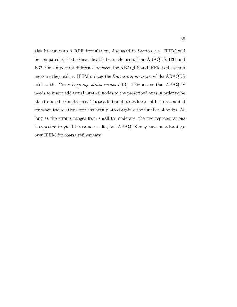
4.1 Three legged beam
The three legged beam consists of three beams connected with 90 degree
angles, in such a manner that each leg’s beam axis is parallel to the x-, y-
and z-axis. The relative error of displacement and rotation is plotted against
the number of free nodes for each leg. The geometry and the beam properties
are depicted in Figure 4.2.
Figure 4.2: Geometry and loading of the three legged beam[15]
The beam is subjected to two concentrated loads, acting in the negative
x- and z-directions. This loading induces shear stress, combined bending
and torsion, and is well suited as a benchmark for testing nonlinear beam
formulations.
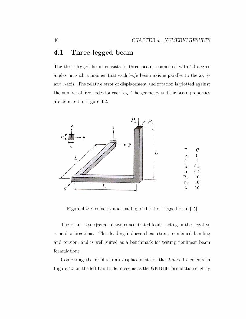
Comparing the results from displacements of the 2-noded elements in
Figure 4.3 on the left hand side, it seems as the GE RBF formulation slightly
4.1. THREE LEGGED BEAM 41
outperforms the unenhanced formulation, and is almost coinciding with the
solution from ABAQUS. However, looking at the rotations on the right hand
side of Figure 4.3, the tables have turned and the unenhanced formulation
now slightly outperforms the RBF formulation, whilst coinciding with the
solution from ABAQUS.
Figure 4.3: Displacement plot on the left and rotation plot on the right sidefor the 2-noded elements
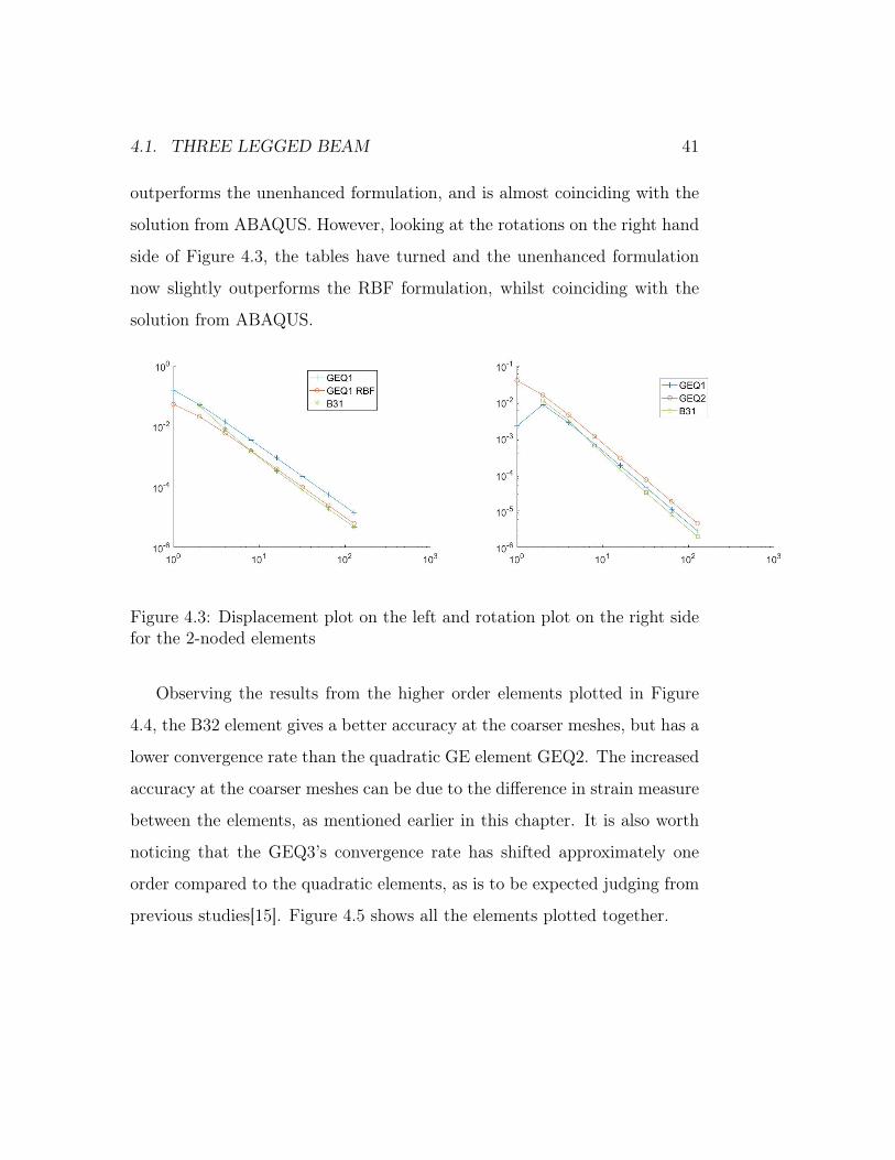
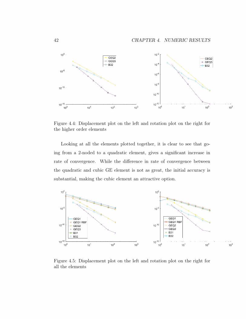
Observing the results from the higher order elements plotted in Figure
4.4, the B32 element gives a better accuracy at the coarser meshes, but has a
lower convergence rate than the quadratic GE element GEQ2. The increased
accuracy at the coarser meshes can be due to the difference in strain measure
between the elements, as mentioned earlier in this chapter. It is also worth
noticing that the GEQ3’s convergence rate has shifted approximately one
order compared to the quadratic elements, as is to be expected judging from
previous studies[15]. Figure 4.5 shows all the elements plotted together.
42 CHAPTER 4. NUMERIC RESULTS
Figure 4.4: Displacement plot on the left and rotation plot on the right forthe higher order elements
Looking at all the elements plotted together, it is clear to see that go-
ing from a 2-noded to a quadratic element, gives a significant increase in
rate of convergence. While the difference in rate of convergence between
the quadratic and cubic GE element is not as great, the initial accuracy is
substantial, making the cubic element an attractive option.
Figure 4.5: Displacement plot on the left and rotation plot on the right forall the elements
4.2. CURVED BEAM 43
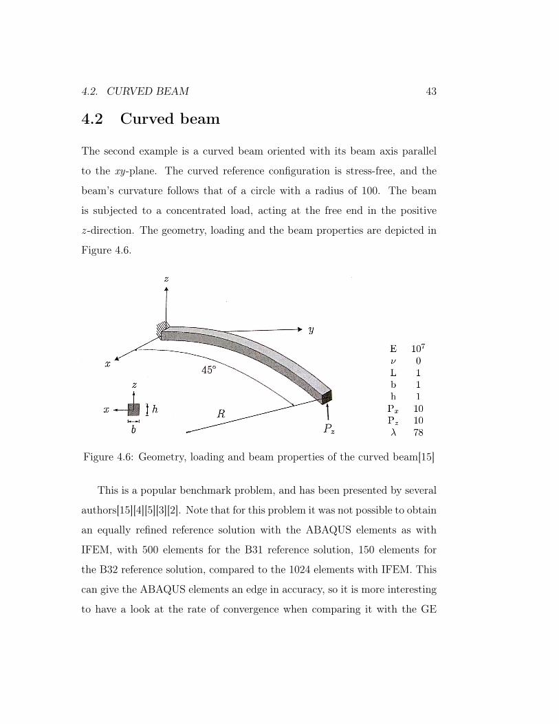
4.2 Curved beam
The second example is a curved beam oriented with its beam axis parallel
to the xy-plane. The curved reference configuration is stress-free, and the
beam’s curvature follows that of a circle with a radius of 100. The beam
is subjected to a concentrated load, acting at the free end in the positive
z -direction. The geometry, loading and the beam properties are depicted in
Figure 4.6.
Figure 4.6: Geometry, loading and beam properties of the curved beam[15]
This is a popular benchmark problem, and has been presented by several
authors[15][4][5][3][2]. Note that for this problem it was not possible to obtain
an equally refined reference solution with the ABAQUS elements as with
IFEM, with 500 elements for the B31 reference solution, 150 elements for
the B32 reference solution, compared to the 1024 elements with IFEM. This
can give the ABAQUS elements an edge in accuracy, so it is more interesting
to have a look at the rate of convergence when comparing it with the GE
44 CHAPTER 4. NUMERIC RESULTS
elements.
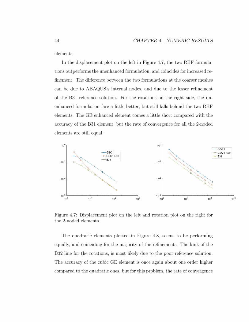
In the displacement plot on the left in Figure 4.7, the two RBF formula-
tions outperforms the unenhanced formulation, and coincides for increased re-
finement. The difference between the two formulations at the coarser meshes
can be due to ABAQUS’s internal nodes, and due to the lesser refinement
of the B31 reference solution. For the rotations on the right side, the un-
enhanced formulation fare a little better, but still falls behind the two RBF
elements. The GE enhanced element comes a little short compared with the
accuracy of the B31 element, but the rate of convergence for all the 2-noded
elements are still equal.
Figure 4.7: Displacement plot on the left and rotation plot on the right forthe 2-noded elements
The quadratic elements plotted in Figure 4.8, seems to be performing
equally, and coinciding for the majority of the refinements. The kink of the
B32 line for the rotations, is most likely due to the poor reference solution.
The accuracy of the cubic GE element is once again about one order higher
compared to the quadratic ones, but for this problem, the rate of convergence
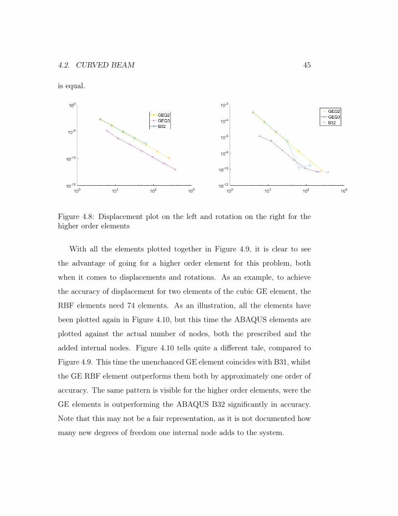
4.2. CURVED BEAM 45
is equal.
Figure 4.8: Displacement plot on the left and rotation on the right for thehigher order elements
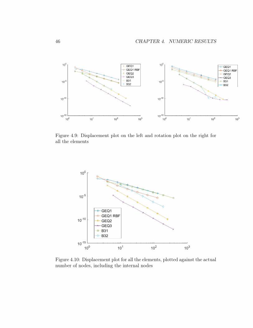
With all the elements plotted together in Figure 4.9, it is clear to see
the advantage of going for a higher order element for this problem, both
when it comes to displacements and rotations. As an example, to achieve
the accuracy of displacement for two elements of the cubic GE element, the
RBF elements need 74 elements. As an illustration, all the elements have
been plotted again in Figure 4.10, but this time the ABAQUS elements are
plotted against the actual number of nodes, both the prescribed and the
added internal nodes. Figure 4.10 tells quite a different tale, compared to
Figure 4.9. This time the unenchanced GE element coincides with B31, whilst
the GE RBF element outperforms them both by approximately one order of
accuracy. The same pattern is visible for the higher order elements, were the
GE elements is outperforming the ABAQUS B32 significantly in accuracy.
Note that this may not be a fair representation, as it is not documented how
many new degrees of freedom one internal node adds to the system.
46 CHAPTER 4. NUMERIC RESULTS
Figure 4.9: Displacement plot on the left and rotation plot on the right forall the elements
Figure 4.10: Displacement plot for all the elements, plotted against the actualnumber of nodes, including the internal nodes
4.3. DYNAMIC 47
4.3 Dynamic
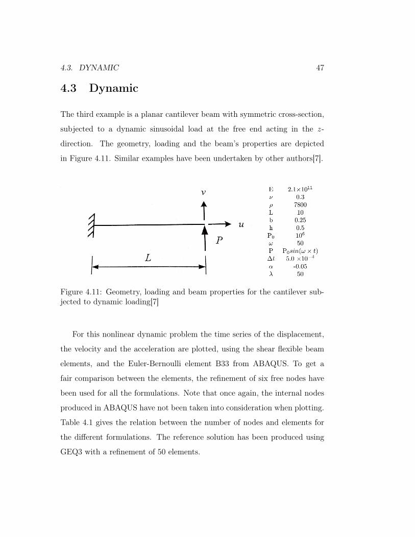
The third example is a planar cantilever beam with symmetric cross-section,
subjected to a dynamic sinusoidal load at the free end acting in the z -
direction. The geometry, loading and the beam’s properties are depicted
in Figure 4.11. Similar examples have been undertaken by other authors[7].
Figure 4.11: Geometry, loading and beam properties for the cantilever sub-jected to dynamic loading[7]
For this nonlinear dynamic problem the time series of the displacement,
the velocity and the acceleration are plotted, using the shear flexible beam
elements, and the Euler-Bernoulli element B33 from ABAQUS. To get a
fair comparison between the elements, the refinement of six free nodes have
been used for all the formulations. Note that once again, the internal nodes
produced in ABAQUS have not been taken into consideration when plotting.
Table 4.1 gives the relation between the number of nodes and elements for
the different formulations. The reference solution has been produced using
GEQ3 with a refinement of 50 elements.
48 CHAPTER 4. NUMERIC RESULTS
GEQ1 GEQ1 RBF GEQ2 GEQ3 B31 B33 B32
Elements 6 6 3 2 6 6 3
Nodes 7 7 7 7 7 7 7
Added nodes 0 0 0 0 12 6 9
Table 4.1: Number of nodes and elements needed for the different elements
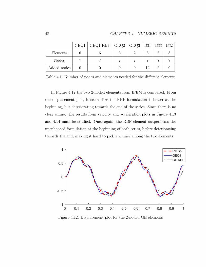
In Figure 4.12 the two 2-noded elements from IFEM is compared. From
the displacement plot, it seems like the RBF formulation is better at the
beginning, but deteriorating towards the end of the series. Since there is no
clear winner, the results from velocity and acceleration plots in Figure 4.13
and 4.14 must be studied. Once again, the RBF element outperforms the
unenhanced formulation at the beginning of both series, before deteriorating
towards the end, making it hard to pick a winner among the two elements.
Figure 4.12: Displacement plot for the 2-noded GE elements
4.3. DYNAMIC 49
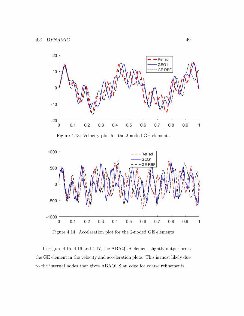
Figure 4.13: Velocity plot for the 2-noded GE elements
Figure 4.14: Acceleration plot for the 2-noded GE elements
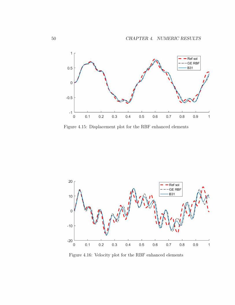
In Figure 4.15, 4.16 and 4.17, the ABAQUS element slightly outperforms
the GE element in the velocity and acceleration plots. This is most likely due
to the internal nodes that gives ABAQUS an edge for coarse refinements.
50 CHAPTER 4. NUMERIC RESULTS
Figure 4.15: Displacement plot for the RBF enhanced elements
Figure 4.16: Velocity plot for the RBF enhanced elements
4.3. DYNAMIC 51
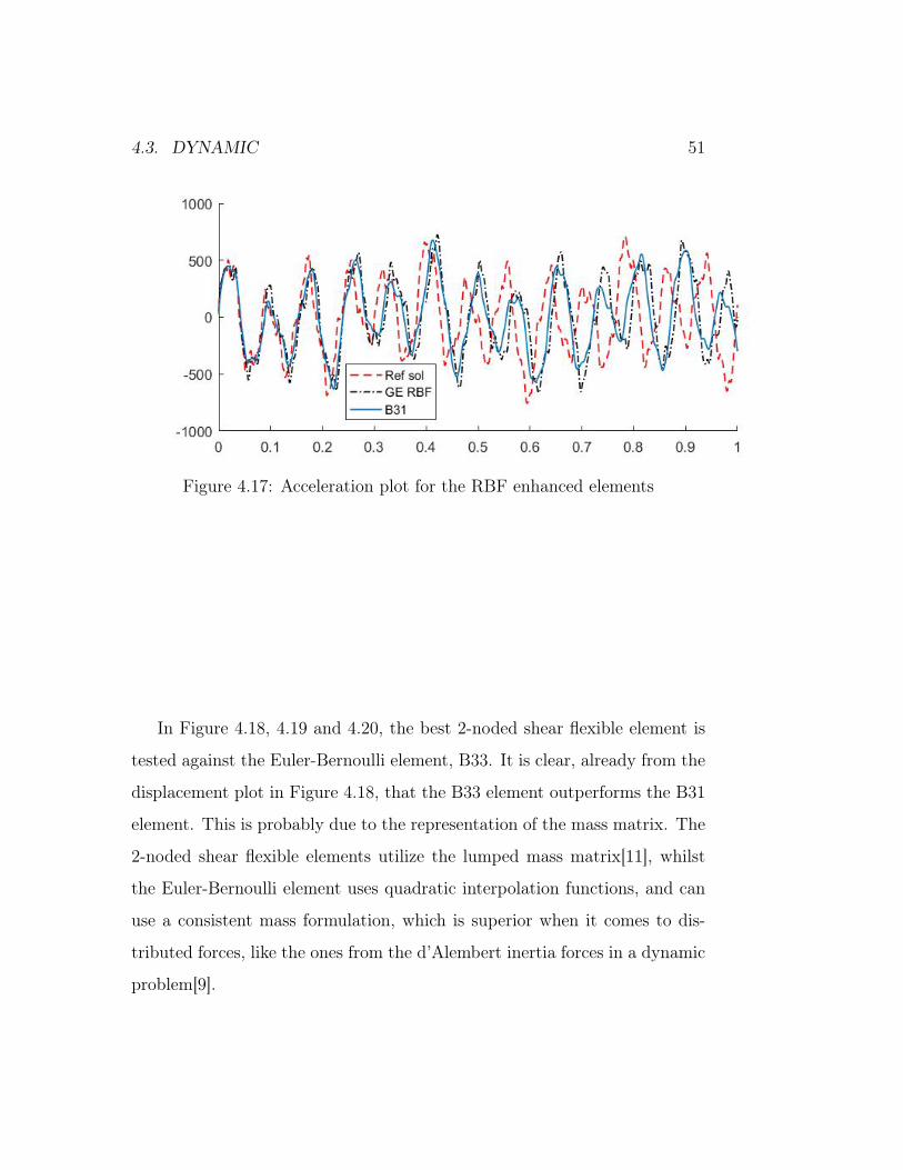
Figure 4.17: Acceleration plot for the RBF enhanced elements
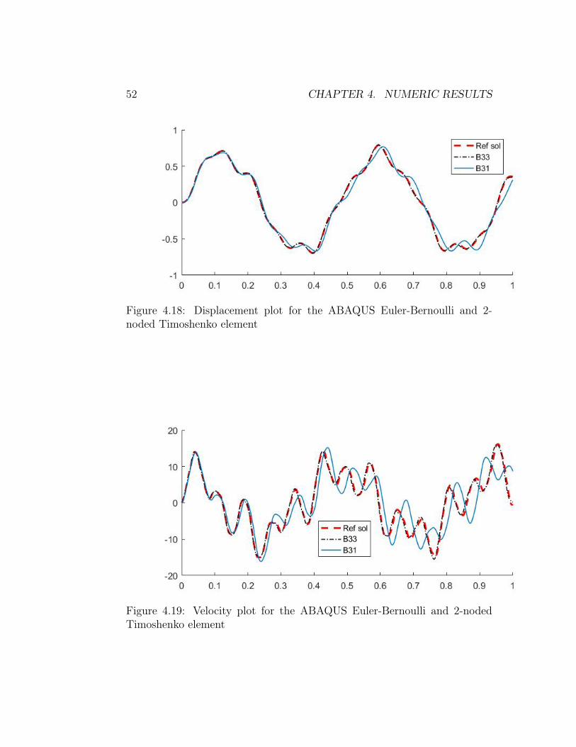
In Figure 4.18, 4.19 and 4.20, the best 2-noded shear flexible element is
tested against the Euler-Bernoulli element, B33. It is clear, already from the
displacement plot in Figure 4.18, that the B33 element outperforms the B31
element. This is probably due to the representation of the mass matrix. The
2-noded shear flexible elements utilize the lumped mass matrix[11], whilst
the Euler-Bernoulli element uses quadratic interpolation functions, and can
use a consistent mass formulation, which is superior when it comes to dis-
tributed forces, like the ones from the d’Alembert inertia forces in a dynamic
problem[9].
52 CHAPTER 4. NUMERIC RESULTS
Figure 4.18: Displacement plot for the ABAQUS Euler-Bernoulli and 2-noded Timoshenko element
Figure 4.19: Velocity plot for the ABAQUS Euler-Bernoulli and 2-nodedTimoshenko element
4.3. DYNAMIC 53
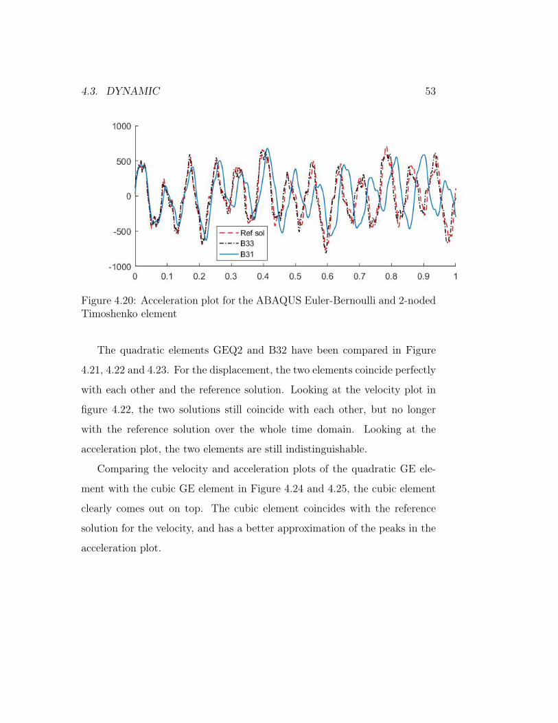
Figure 4.20: Acceleration plot for the ABAQUS Euler-Bernoulli and 2-nodedTimoshenko element
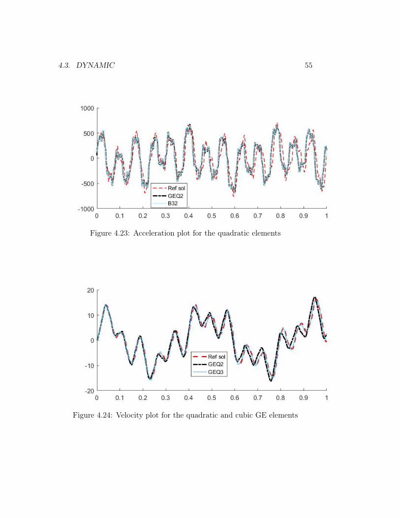
The quadratic elements GEQ2 and B32 have been compared in Figure
4.21, 4.22 and 4.23. For the displacement, the two elements coincide perfectly
with each other and the reference solution. Looking at the velocity plot in
figure 4.22, the two solutions still coincide with each other, but no longer
with the reference solution over the whole time domain. Looking at the
acceleration plot, the two elements are still indistinguishable.
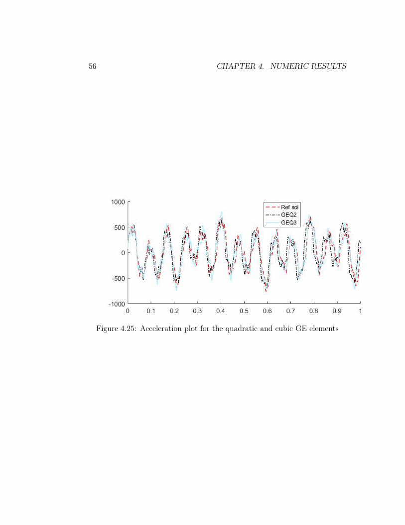
Comparing the velocity and acceleration plots of the quadratic GE ele-
ment with the cubic GE element in Figure 4.24 and 4.25, the cubic element
clearly comes out on top. The cubic element coincides with the reference
solution for the velocity, and has a better approximation of the peaks in the
acceleration plot.

54 CHAPTER 4. NUMERIC RESULTS
Figure 4.21: Displacement plot for the quadratic elements
Figure 4.22: Velocity plot for the quadratic elements
4.3. DYNAMIC 55
Figure 4.23: Acceleration plot for the quadratic elements
Figure 4.24: Velocity plot for the quadratic and cubic GE elements
56 CHAPTER 4. NUMERIC RESULTS
Figure 4.25: Acceleration plot for the quadratic and cubic GE elements

Chapter 5
Summary and Conclusion
In this master thesis a review of the geometrically exact (GE) beam model
presented in [15] for static and dynamic analysis of beam-like 3D struc-
tural problems has been presented. In Chapter 2, the Timoshenko beam
element[17] has been compared to the Euler-Bernoulli element. Chapter 2
also describes the shear locking phenomena and remedies to eliminate it. The
solving of nonlinear equilibrium equations for static and dynamic problems
has been described in Chapter 3, as well as the strain measures utilized by
IFEM and ABAQUS. Chapter 4 presents the numerical results.
In this master thesis the GE beam element, an in-house software devel-
oped by SINTEF ICT, has been compared with the well known and highly
regarded beam elements from ABAQUS. The problems solved in this the-
sis have large displacements and rotations, but small to moderate strains,
making them ideal for comparing the two formulations. The numeric results
shows that the higher order elements perform better both when it comes to
accuracy and rate of convergence for all the problems, thus making them
57

58 CHAPTER 5. SUMMARY AND CONCLUSION
attractive despite of their theoretical and numerical complexity. The results
also shows that enhancing the 2-noded GE beam element with residual bend-
ing flexibility increases the performance. This is in accordance to the findings
made by Kjell M. Mathisen et al.[15]. Further work should entail developing
a GE corotational beam formulation.

Bibliography
[1] On Finite Deformations of Space-curved Beams. J.Appl. Math. Phys.,
pages 734–744, 1981.
[2] Anna Bauer, Michael Breitenberger, B. Phillipp, Roland Wüchner, and
K.U. Bletzinger. Nonlinear Spatial Bernoulli Beam. Comput. Meth.Appl.
Mech. Engrg, pages 101–127, 2016.
[3] P. Betsch and P. Steinmann. Frame-indifferent beam finite elements
based upon the geometrically exact beam theory. Comput. Meth.Appl.
Mech. Engrg, pages 1775–1788, 2002.
[4] A. Cardona and M. Géradin. A Beam Finite Element Non-linear Theory
with Finite Rotations. Int. J. Numer. Meth. Engrg, pages 2403–2438,
1988.
[5] M. A Consistent Corotational Formulation for Non-linear Three-
dimensional Beam Elements Crisfield. A Beam Finite Element Non-
linear Theory with Finite Rotations. Comput. Meth.Appl. Mech. Engrg,
pages 131–150, 1990.
[6] T.J.R Hughes. The Finite Element Method. Prentice-Hall, 1987.
59
60 BIBLIOGRAPHY
[7] Thanh-Nam Le. Nonlinear Dynamics of Flexible Structures Using Coro-
tational Beam Elements. pages 10–13, 2013.
[8] R.H MacNeal. Finite Elements: Their Design and Performance. Marcel
Dekker, 1994.
[9] Abaqus Analysis User’s Manual. 25.3.3 choosing a beam element.
[10] Abaqus Analysis User’s Manual. 3.5.2 beam element formulation.
[11] Abaqus Analysis User’s Manual. 3.5.5 mass and inertia for timoshenko
beams.
[12] Kjell M. Mathisen. Introduction to Nonlinear FEA, 2016.
[13] Kjell M. Mathisen. Solution of Nonlinear Dynamic Equilibrium Equa-
tions, 2016.
[14] Kjell M. Mathisen. Solution of Nonlinear Equilibrium Equations, 2016.
[15] Kjell M. Mathisen, Yuri Bazilevs, Bjørn Haugen, Tore A. Helgedagsrud,
Trond Kvamsdal, Knut M. Okstad, and Siv B. Raknes. A Comparative
Study of Beam Element Formulations for Nonlinear Analysis: Corota-
tional vs Geometrically Exact Formulations. Proceedings of 9th National
Conference on Computational Mechanics (MekIT’17), 2017.
[16] opensees.berkeley.edu. Hilber-hughes-taylor method.
[17] Eugenio Oñate. Structural Analysis with the Finite Element Method.
Linear Statics. Volume 2: Beams, Plates and Shells:37–58, 2013.
BIBLIOGRAPHY 61
[18] Eugenio Oñate. Structural analysis with the finite element method.
linear statics. Volume 2: Beams, Plates and Shells:1–10, 2013.
[19] Roland Wüchner, Michael Breitenberger, and Anna Bauer. Isogeometric
Structural Analysis and Design. Chair of Structural Analysis Technical
University of Munich, 2016.

62 BIBLIOGRAPHY
A IFEM Input Files
63

64 A IFEM INPUT FILES
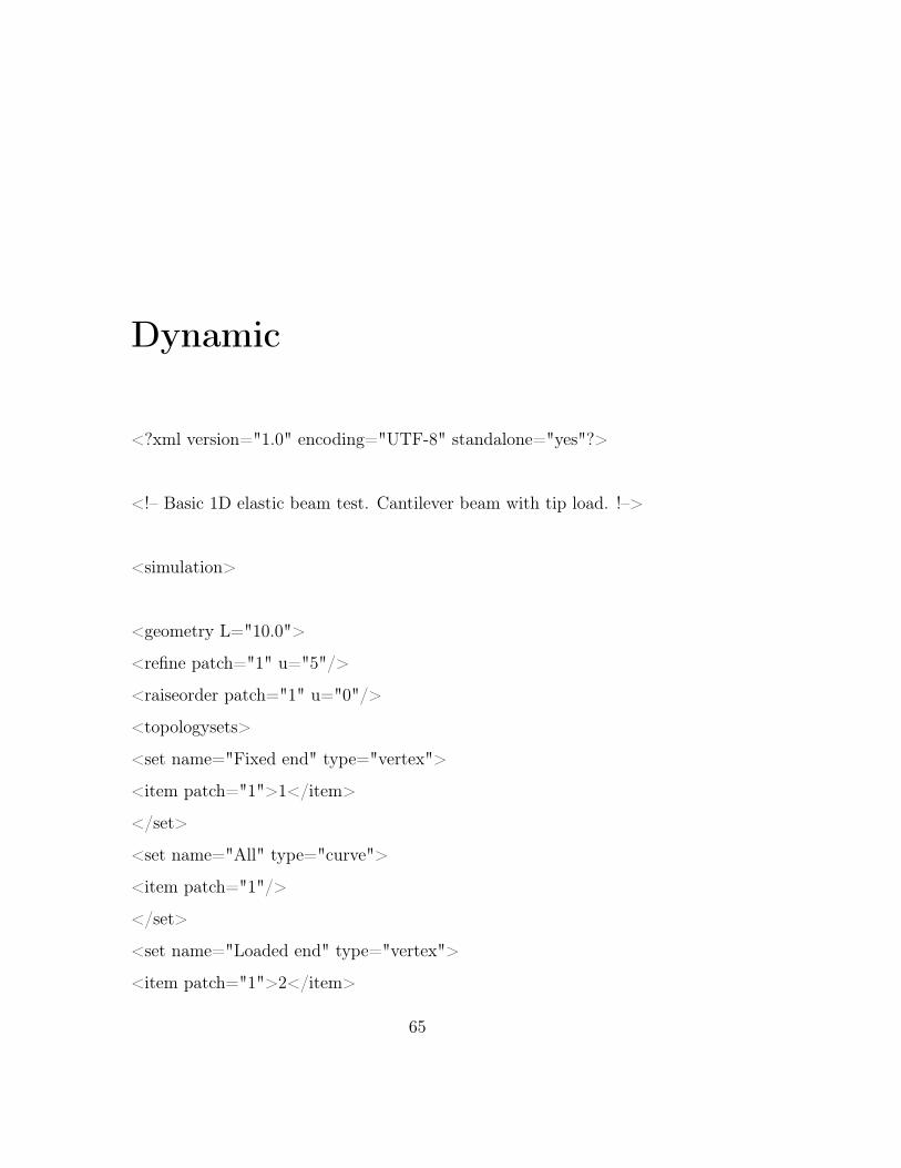
Dynamic
<?xml version="1.0" encoding="UTF-8" standalone="yes"?>
<!– Basic 1D elastic beam test. Cantilever beam with tip load. !–>
<simulation>
<geometry L="10.0">
<refine patch="1" u="5"/>
<raiseorder patch="1" u="0"/>
<topologysets>
<set name="Fixed end" type="vertex">
<item patch="1">1</item>
</set>
<set name="All" type="curve">
<item patch="1"/>
</set>
<set name="Loaded end" type="vertex">
<item patch="1">2</item>
65
66 DYNAMIC
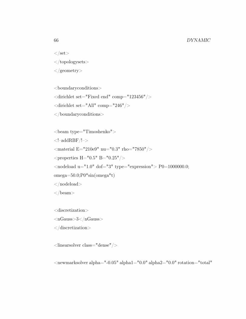
</set>
</topologysets>
</geometry>
<boundaryconditions>
<dirichlet set="Fixed end" comp="123456"/>
<dirichlet set="All" comp="246"/>
</boundaryconditions>
<beam type="Timoshenko">
<!–addRBF/!–>
<material E="210e9" nu="0.3" rho="7850"/>
<properties H="0.5" B="0.25"/>
<nodeload u="1.0" dof="3" type="expression"> P0=1000000.0;
omega=50.0;P0*sin(omega*t)
</nodeload>
</beam>
<discretization>
<nGauss>3</nGauss>
</discretization>
<linearsolver class="dense"/>
<newmarksolver alpha="-0.05" alpha1="0.0" alpha2="0.0" rotation="total"
67
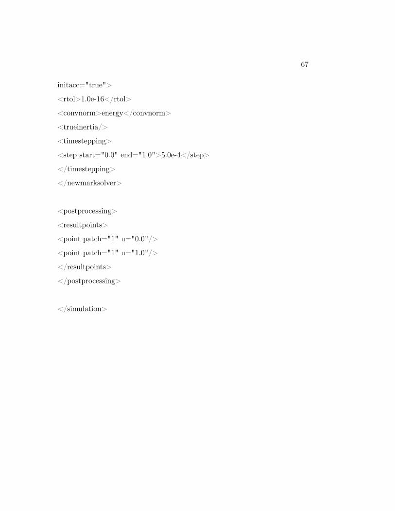
initacc="true">
<rtol>1.0e-16</rtol>
<convnorm>energy</convnorm>
<trueinertia/>
<timestepping>
<step start="0.0" end="1.0">5.0e-4</step>
</timestepping>
</newmarksolver>
<postprocessing>
<resultpoints>
<point patch="1" u="0.0"/>
<point patch="1" u="1.0"/>
</resultpoints>
</postprocessing>
</simulation>

68 DYNAMIC
Three Legged Beam
<?xml version="1.0" encoding="UTF-8" standalone="yes"?>
<!– Basic 1D elastic beam test.
3-segment cantilever with slope discontinuities.
Clamped at one end (at 0,0,0) and a nodal load at the free end. !–>
<simulation>
<geometry>
<patchfile>beamXYZ.G2</patchfile>
<refine lowerpatch="1" upperpatch="3" u="127"/>
<raiseorder lowerpatch="1" upperpatch="3" u="0"/>
<topologysets>
<set name="root" type="vertex">
<item patch="1">1</item>
</set>
<set name="tip" type="vertex">
<item patch="3">2</item>
69
70 THREE LEGGED BEAM
</set>
</topologysets>
</geometry>
<boundaryconditions>
<dirichlet set="root" comp="123456"/>
</boundaryconditions>
<beam type="Timoshenko">
<!–addRBF/!–>
<material E="1.0e6" G="5.0e5"/>
<properties B="0.1" H="0.1"/>
<nodeload patch="3" u="1" dof="1" type="linear">-10.0</nodeload>
<nodeload patch="3" u="1" dof="3" type="linear">-10.0</nodeload>
</beam>
<geometry>
<topology>
<connection master="1" mvert="2" slave="2" svert="1"/>
<connection master="2" mvert="2" slave="3" svert="1"/>
</topology>
</geometry>
<discretization>
<nGauss>3</nGauss>

71
</discretization>
<nonlinearsolver rotation="total">
<timestepping>
<step start="0.0" end="1.0">20</step>
</timestepping>
<rtol>1.0e-16</rtol>
<dtol>1.0e+05</dtol>
<noEnergy/>
</nonlinearsolver>
<postprocessing>
<resultpoints>
<point patch="3" u="1.0"/>
</resultpoints>
</postprocessing>
</simulation>

72 THREE LEGGED BEAM
Curved Beam
<?xml version="1.0" encoding="UTF-8" standalone="yes"?>
<!– Basic 1D elastic beam test. Cantilever arc with tip shear load. !–>
<simulation>
<geometry>
<patchfile>arc45.g2</patchfile>
<refine patch="1" u="127"/>
<raiseorder patch="1" u="0"/>
<topologysets>
<set name="innspenning" type="vertex">
<item patch="1">1</item>
</set>
</topologysets>
</geometry>
<boundaryconditions>
73
74 CURVED BEAM
<dirichlet set="innspenning" comp="123456"/>
</boundaryconditions>
<beam type="Timoshenko">
<material E="1.0e7" G="5.0e6"/>
<properties B="1.0" H="1.0"/>
<nodeload u="1" dof="3" type="linear">600.0</nodeload>
</beam>
<discretization>
<nGauss>3</nGauss>
</discretization>
<nonlinearsolver rotation="total">
<timestepping>
<step start="0.0" end="1.0">0.1</step>
</timestepping>
<rtol>1.0e-16</rtol>
<dtol>1000.0</dtol>
<noEnergy/>
</nonlinearsolver>
<postprocessing>
<resultpoints>
<point patch="1" u="1.0"/>
75
</resultpoints>
</postprocessing>
</simulation>

76 CURVED BEAM

B ABAQUS Input FIles
77

78 B ABAQUS INPUT FILES
Dynamic
*Heading
** Job name: TestBeam Model name: Model-1
** Generated by: Abaqus/CAE 6.12-1
*Preprint, echo=NO, model=NO, history=NO, contact=NO
**
** PARTS
**
*Part, name=Part-1
*Node
1, 0., 0., 0.
7, 10., 0., 0.
*Element, type=B32
1, 1, 2, 3
*Ngen, nset=Set-1
1, 7, 1 *Elgen, elset=Set-1
1, 3, 2, 1
** Section: Section-1 Profile: Profile-1
*Beam General Section, elset=Set-1, density=7850., section=general,
79
80 DYNAMIC
poisson=0.3
1.25e-1, 6.5104167e-4, 0., 2.6041667e-3, 3.90625e-3
0., 1., 0.
2.1e+11, 6.730769232e10
*End Part
**
**
** ASSEMBLY
**
*Assembly, name=Assembly
**
*Instance, name=Part-1-1, part=Part-1
*End Instance
**
*Nset, nset=Set-1, instance=Part-1-1
1,
*Nset, nset=Set-2, instance=Part-1-1
7,
*End Assembly
**
** BOUNDARY CONDITIONS
**
** Name: BC-1 Type: Displacement/Rotation
*Boundary
Set-1, 1, 6

81
*Amplitude, name=sinewave, definition=periodic
1, 50, 0, 0
0, 1
**initial conditions,type=solution,user
** —————————————————————-
**
** STEP: Step-2
**
*Step, name=Step-2, nlgeom=YES, inc=10000000, amplitude=ramp
*Dynamic,direct,nohaf,alpha=-0.05
0.0005, 1.0,
**
** LOADS
**
** Name: Load-2 Type: Concentrated force
*Cload, amplitude=sinewave
Set-2, 3, 1.e+6
**
** OUTPUT REQUESTS
**
*Restart, write, frequency=0
**
** FIELD OUTPUT: F-Output-1
**
*Output, field, frequency=1
82 DYNAMIC
*Node Output
U,
**
** HISTORY OUTPUT: H-Output-1
**
*Output, history, variable=PRESELECT, frequency=1
*Node Print, nset=Set-2
U3, V3, A3
**El print, elset=Part-1-1.Set-1
** nforc
*End Step
Three Legged Beam
*Preprint, echo=NO, model=YES, history=NO, contact=NO
*PART, NAME=PART-1
*NODE
1, 0, 0, 0
257, 1, 0, 0
515, 1, 1, 0
769, 1, 1, 1
*ELEMENT, TYPE=B32
1, 1, 2, 3
*ELEMENT, TYPE=B32
129, 257, 258, 259
*ELEMENT, TYPE=B32
257, 515, 516, 517
*NGEN, NSET=SET-1
1, 257, 1
*NGEN, NSET=SET-2
257, 515, 1
*NGEN, NSET=SET-3
83
84 THREE LEGGED BEAM
515, 769, 1
*ELGEN, ELSET=SET-1
1, 128, 2, 1
*ELGEN, ELSET=SET-2
129, 128, 2, 1
*ELGEN, ELSET=SET-3
257, 128, 2, 1
*BEAM GENERAL SECTION, ELSET=SET-1, DENSITY=7850, SEC-
TION=GENERAL, POISSON=0.0
0.0100000000, 0.0000083333, 0, 0.0000083333, 0.0000200000
0,1,0
1000000.0000000000, 416666.6666666667
*BEAM GENERAL SECTION, ELSET=SET-2, DENSITY=7850, SEC-
TION=GENERAL, POISSON=0.0
0.0100000000, 0.0000083333, 0, 0.0000083333, 0.0000200000
-1,0,0
1000000.0000000000, 416666.6666666667
*BEAM GENERAL SECTION, ELSET=SET-3, DENSITY=7850, SEC-
TION=GENERAL, POISSON=0.0
0.0100000000, 0.0000083333, 0, 0.0000083333, 0.0000200000
-1,0,0
1000000.0000000000, 416666.6666666667
*END PART
*ASSEMBLY, NAME=ASSEMBLY
*INSTANCE, NAME=PART-1-1, PART=PART-1
85
*END INSTANCE
*NSET, NSET=SET1, INSTANCE=PART-1-1
1,
*NSET, NSET=SET2, INSTANCE=PART-1-1
382,
*END ASSEMBLY
** CREATE BC
*BOUNDARY
SET1, ENCASTRE
*STEP, NAME=STEPBC,AMPLITUDE = RAMP, INC = 1000, NLGEOM =
Y ES
∗ STATIC,DIRECT
1e− 3, 1.0
∗ ∗
∗ CLOAD
SET2, 1,−10
SET2, 3,−10
∗ ∗
∗ CONTROLS,RESET
∗CONTROLS, PARAMETERS = FIELD,FIELD = DISPLACEMENT
1e− 04, 1e− 07, , , , , ,
∗ CONTROLS, PARAMETERS = FIELD,FIELD = ROTATION
1e− 04, 1e− 07, , , , , ,
∗RESTART,WRITE, FREQUENCY = 0
∗ ∗Requestdisplacementsandrotations

86 THREE LEGGED BEAM
∗OUTPUT, FIELD
∗NODEOUTPUT,NSET = SET2
U,UR
∗ ∗
∗ ENDSTEP
Curved Beam
*Heading
** Job name: TestBeam Model name: Model-1
** Generated by: Abaqus/CAE 6.12-1
*Preprint, echo=YES, model=YES, history=NO, contact=NO
**
** PARTS
**
*Part, name=Part-1
*Node
1, 0., 0., 0.
9, 29.2893218813452, 70.7106781186547, 0.
10, 100., 0., 0.
*Element, type=B31
1, 1, 2
*Ngen, nset=Set-1, LINE=C
1, 9, 1, 10
*Elgen, elset=Set-1
1, 8, 1, 1
87
88 CURVED BEAM
** Section: Section-1 Profile: Profile-1
*Beam General Section, elset=Set-1, density=7850., section=GENERAL,
poisson=0.0
1., 8.333333333333333e-2, 0., 8.333333333333333e-2, 1.7e-1
-1., 0., 0.
1.e+7, 4.901960785e+6
*End Part
**
**
** ASSEMBLY
**
*Assembly, name=Assembly
**
*Instance, name=Part-1-1, part=Part-1
*End Instance
**
*Nset, nset=Set-1, instance=Part-1-1
1,
*Nset, nset=Set-2, instance=Part-1-1
501,
*End Assembly
**Amplitude, name=sinewave, definition=periodic
** 1, 50., 0., 0.
** 0., 1.e+7
**

89
** BOUNDARY CONDITIONS
**
** Name: BC-1 Type: Displacement/Rotation
*Boundary
Set-1, ENCASTRE
**initial conditions,type=solution,user
** —————————————————————-
**
** STEP: Step-1
**
*Step, name=Step-1, nlgeom=YES, inc=1000000
*Static
.01, 1.0
**
** LOADS
**
** Name: Load-2 Type: Concentrated force
*Cload
Set-2, 3, 600.
**
** CONTROLS
**
*Controls, reset
*Controls, parameters=field, field=displacement
1e-06, 1e-09, , , , , ,
90 CURVED BEAM
*Controls, parameters=field, field=rotation
1e-06, 1e-09, , , , , ,
**
** OUTPUT REQUESTS
**
*Restart, write, frequency=0
**
** FIELD OUTPUT: F-Output-1
**
*Output, field, frequency=1
*Node Output
U,
**
** HISTORY OUTPUT: H-Output-1
**
*Output, history, frequency=1
*Node Output, nset=Set-2
U,
*Node Print, nset=Set-2
U1,U2,U3,UR1,UR2,UR3
*El print, elset=Part-1-1.Set-1
nforc
*End Step